Boreal Forest Snow Damage Mapping Using Multi-Temporal Sentinel-1 Data


1
Department of Electronics and Nanoengineering, Aalto University, P.O. Box 11000, FI-00076 AALTO, 02150 Espoo, Finland
2
VTT Technical Research Centre of Finland, P.O. Box 1000, FI-00076 VTT, 02150 Espoo, Finland
*
Author to whom correspondence should be addressed.
Remote Sens. 2019, 11(4), 384; https://0-doi-org.brum.beds.ac.uk/10.3390/rs11040384
Submission received: 28 December 2018
/
Revised: 2 February 2019
/
Accepted: 8 February 2019
/
Published: 13 February 2019
(This article belongs to the Special Issue Remote Sensing of Boreal Forests)
Abstract
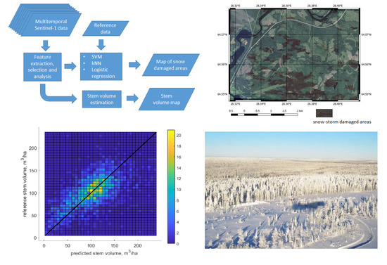
:Natural disturbances significantly influence forest ecosystem services and biodiversity. Accurate delineation and early detection of areas affected by disturbances are critical for estimating extent of damage, assessing economical influence and guiding forest management activities. In this study we focus on snow load damage detection from C-Band SAR images. Snow damage is one of the least studied forest damages, which is getting more common due to current climate trends. The study site was located in the southern part of Northern Finland and the SAR data were represented by the time series of C-band SAR scenes acquired by the Sentinel-1 sensor. Methods used in the study included improved k nearest neighbour method, logistic regression analysis and support vector machine classification. Snow damage recordings from a large snow damage event that took place in Finland during late 2018 were used as reference data. Our results showed an overall detection accuracy of 90%, indicating potential of C-band SAR for operational use in snow damage mapping. Additionally, potential of multitemporal Sentinel-1 data in estimating growing stock volume in damaged forest areas were carried out, with obtained results indicating strong potential for estimating the overall volume of timber within the affected areas. The results and research questions for further studies are discussed.
1. Introduction
Forest ecosystems worldwide are still undergoing significant changes caused by several factors, both natural and anthropogenic. It has been suspected that climate change is one reason, e.g., for more frequent wind storm and snow damage [1]. Poor management and over use of resources in some regions and under use in other regions, e.g., in many European countries are examples of anthropogenic factors. The forest area is increasing in some parts of the globe while at the same time forests are still cleared for other land use, e.g., agricultural land or built-up land. Disturbance assessment and monitoring are important aspects in sustainable management of forests and in efforts to improve our knowledge in ecological processes. Robust methods are needed to quantify and map impacts resulting from various disturbance types including long-term stress, sudden high impact stress, and effect on forest management operations. In this paper, we concentrate on the evaluation of special case of forest structural disturbance, caused by severe snow-load damage that took place between December 2017 and early January 2018 in Finland. A possible effect of the ongoing climate change on the heavy snow-fall in a connection of heavy wind may make the damage more common in the future.
1.1. Snow-Load Damage in 2017–2018
Severe and well documented snow-load damage (referred as snow damage below) on trees and forest stands took place in a large area in East and North Central Finland in the winter 2017–2018. The damage inflicted to forest was considerable, however, varied by extent and severity from area to area. In some areas, all tree trunks had been snapped, while in others, trees were bent in an arc with their crowns frozen at ground level or held by other tree crowns. Over large areas, damage consisted of broken branches and tree bending or lean. Sanitary cuttings have been reported in area of about 6000 hectares by the mid of April 2018. The area of severe damage and needed cutting have been estimated to be about 16,000 hectares. Economical losses are caused by the cuttings that are made earlier than planned and being optimal as well as the decrease in the current total volume of timber. The early cuttings decrease both the current and coming volume of saw timber and pulp wood due to the broken stems and non-optimal timing of cut. The Finnish Forest Centre assessed the economical losses of the land owners to be between 7 to 10 million Euros based on the known situation in the middle of May 2018 [2]. If not otherwise stated, the term volume means here growing stock volume which is the total stem volume of living trees above a certain threshold (the height at least 1.35 m here) in an area of question. All these three terms are used here.
Due to the magnitude of the damage, both ecologically and economically, questions arose whether the affected area of the snow-load damaged forest could be assessed and mapped objectively using remote sensing, and other available environmental data.
In addition to the lost timber volume, insect damage may cause further economical losses if the broken trees are not be removed from forests by the mid of the subsequent summer. Rapid cutting regimes are therefore important. This, on the other hand, presumes rapid mapping of the damaged forests. Space-borne remote sensing data could be the most cost-efficient information source. In the Boreal region, where the damage is frequent, in addition to mountainous areas, e.g., in Central Europe, the only feasible space-borne data are SAR data because of frequent cloud cover during the winter season.
1.2. Related Studies
Sudden and multiple within-year disturbance events can be separated only by frequent monitoring. Such monitoring can be cost effective over large areas if remote sensing technologies are used. Indeed, in recent decades, forest disturbance has received considerable attention from researchers that use remote sensing; however they have been covering mostly wind damage and using optical data. Particularly before launching Sentinel-1 satellites [3], the lack of long synthetic aperture radar (SAR) time series, acquired from sensors with medium-to-high-resolution, has hindered the development of multi-temporal algorithms using active radar sensors, suitable for winter season monitoring.
To date, to the best of our knowledge, very little has been done for assessing specifically crown snow-load damage using space-borne SAR data. Furthermore, remote sensing imagery have been used more often to identify storm damage and controlled felling rather than snow-load damage. As similar change detection methodologies could be employed in principle, we further analyze work on assessment of forest damage caused by storms using SAR. We start with LiDAR and other 3D studies either in storm or snow damage mapping, cite then a few damage studies using optical area sapce-borne data, and further proceed to detection of storm-damaged or other forest change areas using SAR, also logging areas.
Vastaranta et al. [4] used structural changes in forest canopies provided by multi-temporal LiDAR data and demonstrated the usability of area-based estimation method for snow damage assessment. The study was done in connection with snow damage that took place in southern Finland in winter 2009–2010. Snow load resulted in broken, bent and fallen trees changing the canopy structure. The damage was documented at the tree level on permanent field plots. Change features of bi-temporal LiDAR point height distributions were used as predictors in combination with in situ training data. Dense LiDAR data from 2007 and 2010 were used in the analyses. A 5 m × 5 m grid was established in one Scots—Norway spruce stand and change metrics from the LiDAR point height distribution were extracted for the cells. Cells were classified as damaged (n = 43) or non-damaged (n = 42) based on the field data. Stepwise logistic regression detected the damaged cells with an overall accuracy of 78.6%.
Honkavaara et al. [5] developed an automatic method for storm damage detection based on comparisons of digital surface models (DSM). The after-storm DSM was derived using automatic image matching and high-altitude photogrammetric imagery. The DSM was compared to a before-storm DSM, which was computed using national airborne laser scanning (ALS) data.
In [6], the effects of a catastrophic blow-down event in northern Minnesota, USA were assessed using field inventory data, aerial sketch maps and satellite image data processed through the North American Forest Dynamics programme. Estimates were produced for forest area and net volume per unit area of live trees pre- and post-disturbance, and for changes in volume per unit area and total volume resulting from disturbance. Satellite image-based estimates of blow-down area were similar to estimates derived from the inventory plots and aerial sketch maps. Overall accuracy of the image-based damage classification was over 90%. Compared to field inventory estimates, image-based estimates of post-blow-down mean volume per unit area were similar, but estimates of total volume loss were substantially larger.
Einzmann et al. [7] presented a two-step change detection approach applying RapidEye data at 5 m pixel resolution to spot forest damage caused by storm. An object-based bi-temporal change analysis was carried out to identify wind-throw areas larger than 0.5 ha. A supervised Random Forest classifier was used including a semi-automatic feature selection procedure. A large-scale mean shift algorithm was chosen for image segmentation. The object-based change detection approach identified over 90% of the wind-throw areas (larger than 0.5 ha).
SAR-based mapping of forest disturbance has largely been based on two-date change-detection techniques [8,9,10,11,12,13,14,15,16,17,18]. These studies, mostly focused on detecting and mapping fire and logging induced disturbances in forests, show that X-, C- and L-bands are most sensitive SAR wavelengths for detecting disturbance effects in forested landscapes and that the sensitivity does not change across environments, but depend more on resolution and imaging mode. In contrast, wind induced disturbance has been less considered, with only a few SAR-based studies being available [19,20,21]. Suitable sensors were ALOS PALSAR (Advanced Land Observing Satellite Phased Array type L-band Synthetic Aperture Radar), RADARSAT-2, TerraSAR-X.
While there is a common understanding that L-band SAR imagery is most suitable for extracting forest parameters, such as particularly forest stem volume, its major limitation for forest disturbance mapping is absence of frequent acquisitions throughout the year. There is also some evidence that time series of C-band SAR data or high-resolution X-band scenes can work as well or better under certain conditions.
One notable study [19] focused on investigation and evaluation of wind-thrown forest mapping using data from three SAR sensors at the coniferous dominated boreal test site. The satellite data consisted of time series of HH-pol ALOS PALSAR images, RADARSAT-2 and TerraSAR-X. The results of bitemporal change analysis suggest that stripmap ALOS PALSAR images were less suitable for detecting wind-thrown forest, probably due to too coarse spatial resolution. In contrast, the wind-thrown forest was clearly visible in the RADARSAT-2 and TerraSAR-X HH polarized images, implying that it may be possible to develop an operational tool for mapping of wind-thrown forests. F urthermore, it has been shown recently that multi-temporal composites of C-band SAR images acquired before and after the forest disturbance can be useful in localization of disturbed areas [11,22].
In this study, we capitalize on Sentinel-1 ability to gather long and frequent time series of SAR data, and extend the prior work on C-band time series, with a focus on mapping snow-load effected areas and estimating the affected volume.
1.3. Goal of the Study
The objective of this study is to develop and test methods for detecting and mapping crown snow-load damage of trees using Sentinel-1 time series data.
The specific objectives include:
- to investigate SAR features that are most useful in the prediction of snow damage;
- to investigate what level of accuracy in snow damage mapping can be reached using Sentinel-1 SAR image time series;
- to study what techniques, including support vector machine (SVM), improved k nearest neighbors (ik-NN), and logistic regression (LR) are most applicable for classification of snow damaged forest areas using Sentinel-1 time series data;
- to test the performance of Sentinel-1 data in estimating the volume of growing stock when using well-known improved k-NN estimation method and regression analysis;
- to discuss the methods to be developed to estimate yield gross damage by combining stem volume estimates from Sentinel-1 data with snow damage area.
To the best of our knowledge, this type of assessment with C-band SAR time series data is the first such study.
2. Data
2.1. Study Site
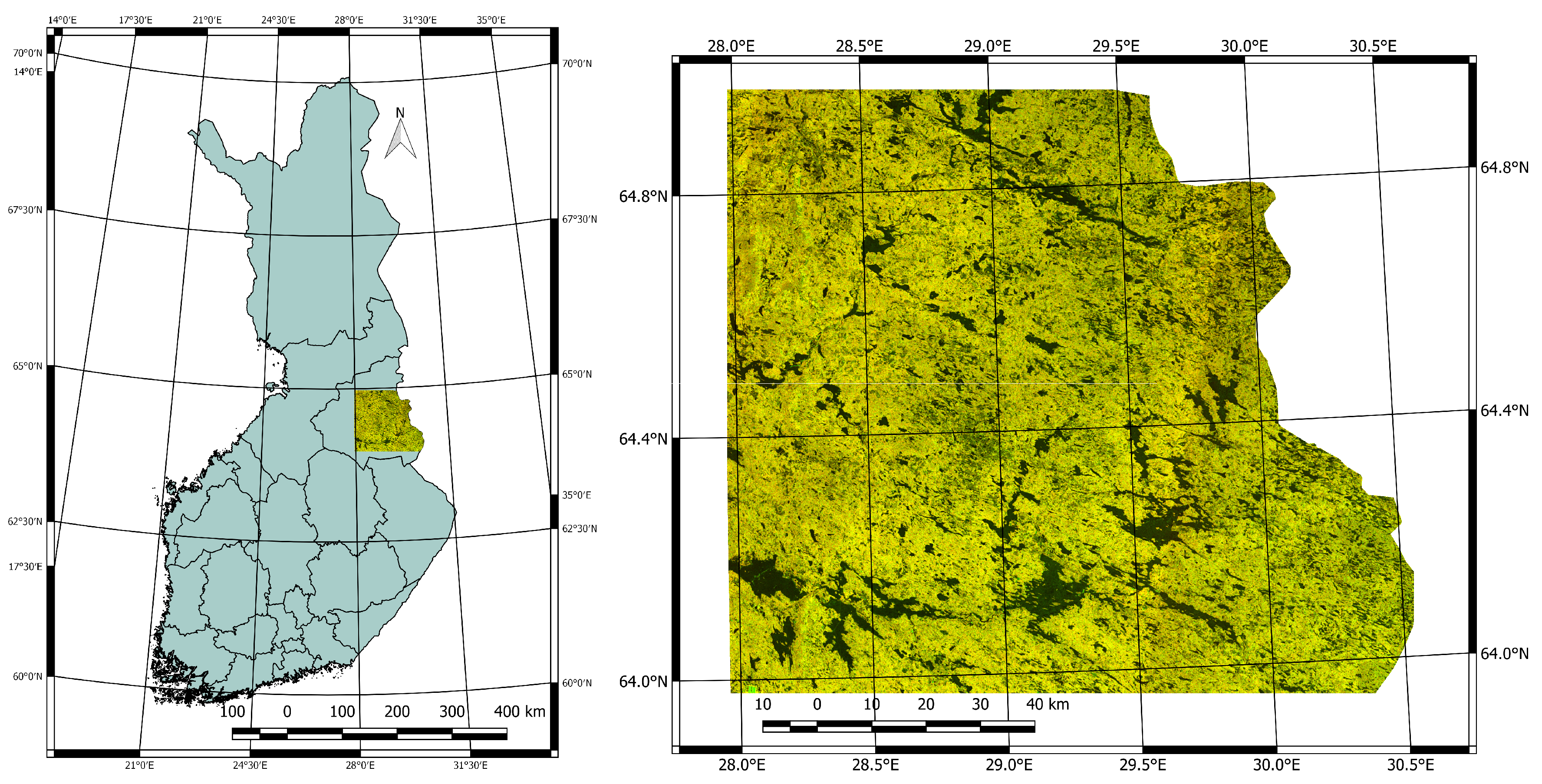
A representative area for crown snow-load damage was selected from the south-eastern part of Northern Finland, in collaboration with the forest authorities at the Finnish Forest Centre. The size of the area, and its exact location were selected to fit the extent of one Sentinel-1 scene. The chosen area is located between latitudes 635848–650802 and longitudes 271206–303508 as shown in Figure 1.
2.2. Sentinel-1 Data
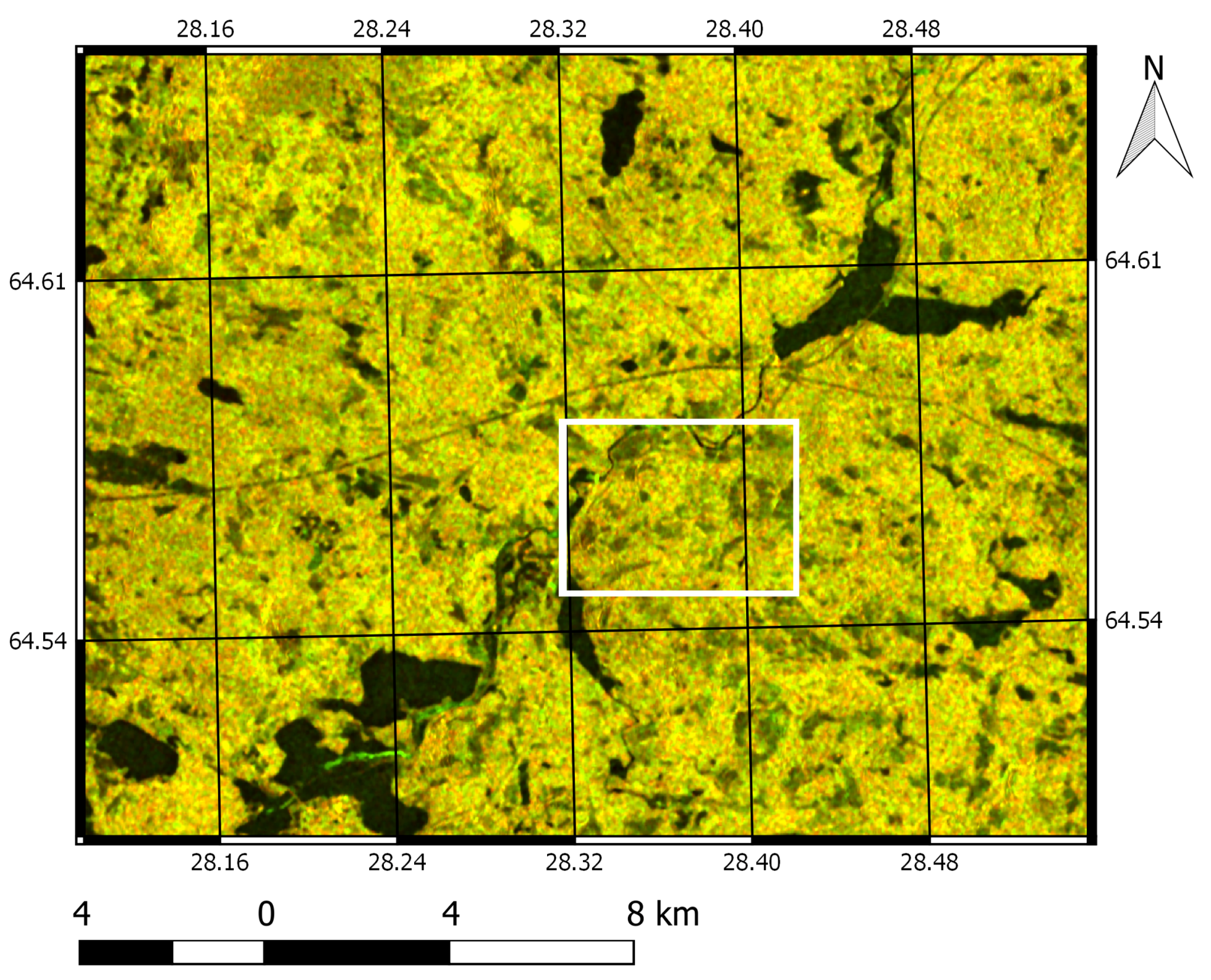
Twelve Sentinel-1 images, Level-1 data with VV and VH polarizations, were downloaded from ESA Open Access Hub. The reasons to use multi-temporal data also in volume estimation is to reduce the effect of the random scattering (speckle) on the estimates and error estimates and also to use the variation of the data acquisition conditions in the estimation through using multifaceted information. The dates of the images are shown in Table 1. An example of colour composition of one Sentinel-1 scene is shown in Figure 2.
The pixel spacing of ortho-rectified scenes was set to 16 m using digital elevation model (DEM), see Section 2.4. Scenes were aggregated in azimuth and range to obtain images with pixel dimensions approximately corresponding to the 20 m grid spacing. Bi-linear interpolation method was used for resampling in connection with the ortho-rectification. Radiometric normalization of intensity was done using a projected pixel area based approach to minimize the effect of the topography. The scenes with a pixel size of about 13.5 m were further re-projected to the ERTS89/ETRS-TM35FIN projection (EPSG:3067) and resampled to a final pixel size of 16 m.
2.3. Ground Reference Data
Altogether, three types of ground data or reference data were available. The first set is the sanitary cutting reports, cutting caused by snow damage, and provided by the Finnish Forest Centre, called here snow damage data (SD data). Another data set was the stand level forest resource data constructed and intended for forest management (MI data). MI data are updated annually based on the reported forestry regimes and should be up-to-date. Some regimes may be missing, however. Furthermore, pixel level estimates from multi-source national forest inventory (MS-NFI data) [23] were used as training data in stem volume estimation.
In total, 929 damaged stands were felled in the selected study area, derived from Sentinel-1 images selected by the mid of April 2018. The size of the cutting areas varied from 0.1 hectares to 64 hectares, the average being 3.25 hectares and the median 3.24 hectares. Please note that some of the area cut may have not had severe damage or damage at all, that is, the area cut around a damaged area cut may have been larger than the damaged area only.
A sample from the MI data was picked up for the reference data without damage. The sample size was 2805 stands. The sizes varied from 0.1 hectares to 18.0 hectares, the average being 1.72 hectares and median 1.20 hectares. A sample from all stands was taken in order to get a balanced reference data. Stand level variables ‘Maturity class’ and ‘Dominant tree species’ were extracted from SD data and MI data.
Some forest variables were missing from the SD and MI data therefore also data from the Finnish Multi-source national forest inventory (MS-NFI) were used as the training data in growing stock volume estimation [24,25]. Another reason was that MS-NFI was more up-to-date. The most recent one for this study was from year 2015 [23]. Furthermore MS-NFI includes more variables than MI data. The pixel level estimates in raster format were available for 45 variables. The pixel size is 16 m × 16 m. The relative RMSE’s of the MS-NFI volume estimates vary between 30% and 40%, depending on the stand size, and at a level of 100 ha between 14% and 15% [26].
The following variables were selected and the averages or weighted averages calculated for both SD and MI stands:
- 1
- Stand mean diameter of trees (cm), average over the stand pixels.
- 2
- Stand mean height of trees (dm), weighted average over the stand pixels, the weight being the basal area of the trees.
- 3
- Stand mean age (years), weighted average over the stand pixels, the weight being the basal area of the trees.
- 4
- Dominant tree species, median over the stand pixels pixel level variable was not available but calculated as follows: (a) selection between coniferous and broad-leaved trees was done based on majority of stem volume, (b) if coniferous, selection between Scots pine and Norway spruce was done based on the majority of stem volume (c) if broad-leaved trees, selection between birch and other broad-leaved trees was done based on the majority of stem volume.
- 5
- Basal area of trees (m/ha), average over the stand pixels.
- 6
- Stem volume of all trees (m/ha), average over the stand pixels.
- 7–8
- Stem volume of Scots pine (Pinus sylvestris L.), Norway spruce (Picea abies Karst.), birch (Betula spp.) and other broad leaved trees, mainly aspen (Populus tremula L.) and alder (Alnus spp.) (m/ha), average over the stand pixels.
2.4. Other Data Sets
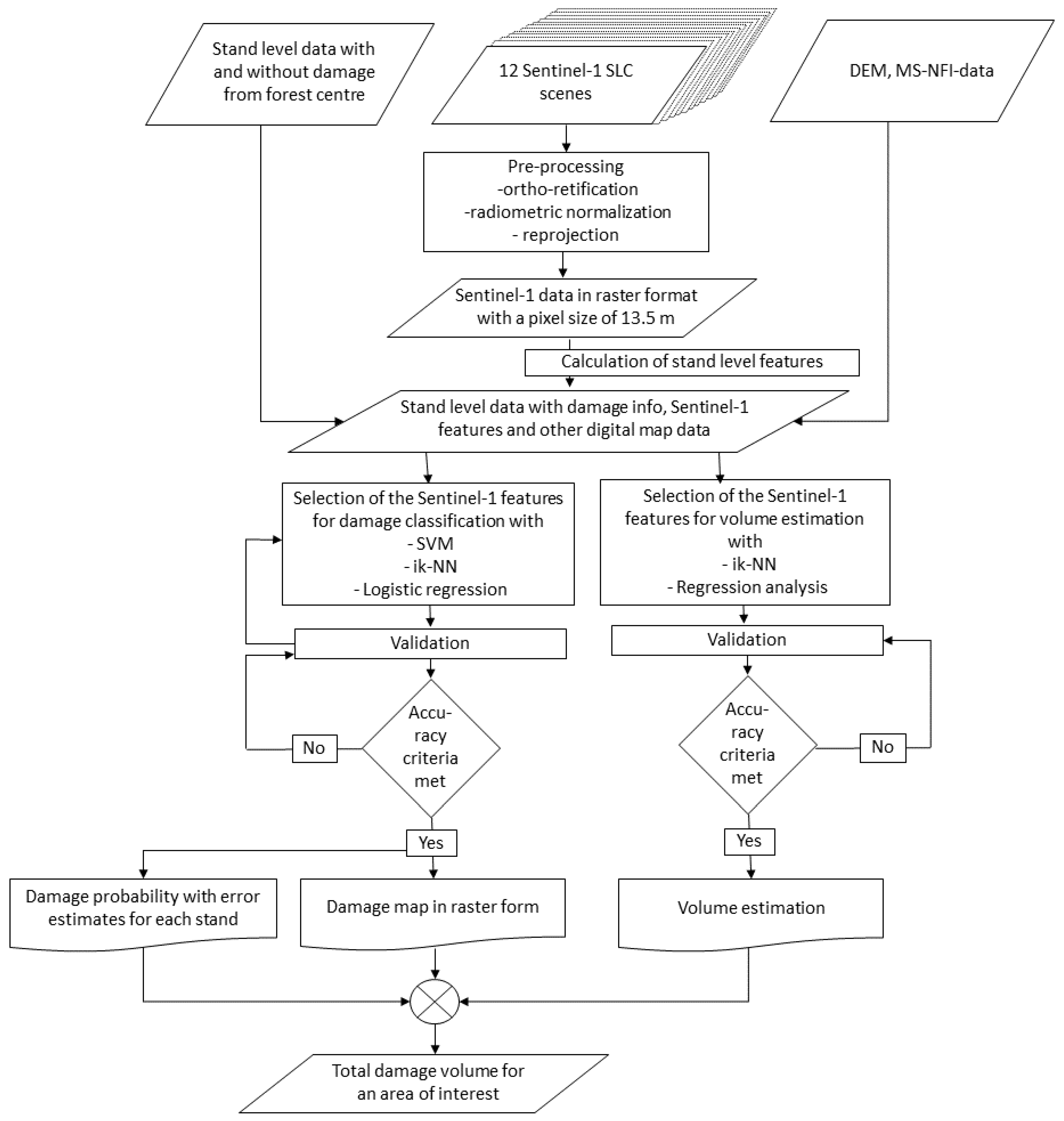
Furthermore, average terrain elevation was calculated for each SD and MI stand using the data from Land Survey Finland. The original pixel size is 10 m × 10 m and elevation resolution 10 cm [27]. The DEM was re-sampled to 16 m pixel spacing using cubic splines. All stands were inside the forest land therefore any additional land use information was not needed. All data sets with the methods are shown in Figure 3.
3. Methods
3.1. Approach
In this study, we concentrate on mapping the extent of the forest area affected by snow load damage and do not explicitly quantify the severity of the damage (i.e., damaged stem volume). Additionally, as a hint for the latter, we perform estimation of growing stock volume, originally available in the study area, testing the capability of Sentinel-1 time series for volume estimation. This, in principle, can help to estimate the amount of growing stock volume present in the area and assess the potential economical losses.
Three different classification methods were elaborated and tested in this study, namely logistic regression analysis for binary data (LR), an improved k-NN method (ik-NN) for categorical variables [28], and support vector machine (SVM) [29]. Several different sets of the predictor variables were tested.
Logistic regression is often used for predicting categorical variables, both binary and multinomial variables when using explanatory variables derived from remote sensing data (e.g., [30]). As a parametric method, it expresses the relationship between an outcome variable (label) and each of its predictors (features). It does not assume a normally distributed error term and is thus robust, but may require more observations than for example discriminant analysis.
The improved ik-NN estimation was developed by Tomppo and Halme [24] and modified for categorical variables with different accuracy metrics as described in [28]. The k-NN method and its variants are widely used in remote sensing applications and in the NFI production in different countries [31]. It was particularly adapted and adjusted here for categorical, binary classification.
SVM is a powerful classification tool, which exhibits low sensitivity to high dimensionality. It has become a popular approach providing improved classification accuracy over other widely used machine learning and pattern recognition techniques. In fact, for a long time, SVM-based classifiers have been the mainstream methods of remote sensing imagery classification [32].
The flowchart of the work-flow of the study is shown in Figure 3. Furthermore, we proceed with description of three methods for classification of snow damaged areas, and also describe methodologies for volume estimation from multiple Sentinel-1 images.
3.2. SAR Metrics Used in the Forest Status Assessment
The SAR features were calculated for each cutting stand and forest management stand separately to remove the effect of speckle and radiometric variation within the stand area for both polarizations. Several different sets of predictor variables were tested, stand-averaged intensities (Equation (1)), standard deviations (Equation (2)) and different ratio images (Equation (3)). From the pixel level intensities (), these backscatter features were calculated for each stand, s, for both polarizations and for each image, k, as follows:
(a) averages,
where is the number of the pixels in stand s,
(b) standard deviations
(c) ratios,
The images are indicated in (Table 1).
3.3. Methods for Snow Damage Classification
3.3.1. Support Vector Machine (SVM) Method
SVM is a machine learning technique presently actively adopted in remote sensing [33,34,35,36]. Support vector machines (SVMs) are supervised learning models with associated learning algorithms that analyze data used for classification or regression. Given a set of training examples, each marked as belonging to one or the other of two categories, an SVM training algorithm builds a model that assigns new examples to one category or the other, making it a non-probabilistic binary linear classifier [29].
SVM are based on statistical learning theory and have the aim of determining the location of decision boundaries that produce the optimal separation of classes [37]. In the case of a two-class pattern recognition problem with linearly separable classes, the SVM selects from among the infinite number of linear decision boundaries the one that minimizes the generalization error. Thus, the selected decision boundary will be the one that leaves the greatest margin between the two classes, where margin is defined as the sum of the distances to the hyperplane from the closest points of the two classes [37]. Margin maximization is achieved using standard quadratic programming optimization techniques. The data points that are closest to the hyperplane are used to measure the margin and are referred to as support vectors.
If the two classes are not linearly separable, the SVM tries to find the hyperplane that maximizes the margin while, at the same time, minimizing a quantity proportional to the number of misclassification errors. The trade-off between margin and misclassification error is controlled by a user-defined constant [29]. SVM can also be extended to handle nonlinear decision surfaces by projecting the input data onto a high-dimensional feature space using kernel functions [37]. Radial basis functions with accordingly selected parameters are a typical choice to serve as kernel functions [33,34].
As SVM are designed for binary classification, this method appears to be an ideal fit for outlier detection problems, such as e.g., separating damaged forest class against intact using temporal dynamics of SAR backscatter. However, for estimating severity of damage (evaluating “change magnitude”) the approach is less suitable.
3.3.2. ik-NN Method for Snow Damage Classification
The well-known k-NN estimation method was also employed in snow damage identification. The weights for the features selected were calculated using genetic algorithm [24,25] and its variant for categorical variables [28]. This k-NN method is called the ik-NN method here.
Let’s recall the main features of the ik-NN estimation with the genetic algorithm in the feature weighting. Denote the k nearest feasible field stand by . The weight of field stand i to pixel p is defined as
The value of k was fixed to be 5 after preliminary tests using the RMSEs and mean deviations as the criteria. The distance weighting power t is a real number, usually . The value was used here. A small quantity, greater than zero, is added to d when and .
The distance metric d employed was
where is the lth SAR feature variable for stand p, the number of SAR feature variables, and the weight for the lth SAR feature variable.
The values of the elements of the weight vector were selected with a genetic algorithm. The details of the genetic algorithm employed are given in [24] and the modification to categorical variables in [25].
The fitness function for the categorical variables to be minimized with respect to vector was
where is a user defined coefficient, an error matrix, the accuracy metric with response variable j whose classes are to be predicted, is the number of response variables to be considered in the optimization procedure and is the weight vector to be optimized (Equation (5)).
For categorical variables, the mode or median of the predicted classes for the nearest neighbours can be used as a prediction instead of a weighted average as is used for continuous variables. For this study, the mode was selected based on earlier investigations [28]. The predicted class has the greatest sum of the weights, , when added by class over the k nearest neighbours. In theory, equal sums are very rare when weights are used; in fact, the probability is zero if rounding is not considered. In cases of equal sums for two or more classes, one class is selected randomly from among those with the greatest sum. This method was used for predicting the categorical variable obtaining the values (0,1) = (non-damaged, damaged).
3.3.3. Logistic Regression Method
Logistic regression was tested as one optional method. The probability that stand p is damaged given the SAR feature vector is expressed as
where is a function of the feature vector whose parameters have to be estimated. A linear function of the feature variables were used for .
3.4. Methods for Growing Stock Estimation
3.4.1. ik-NN Method for Volume Estimation
An interesting question is also what is the severity of the damage, that is what is the stem volume of the broken trees. Some tests for assessing the growing stock volume using Sentinel-1 time series were carried out. Stand level ground truth data was calculated from pixel level data using output volume map of the Finnish national forest inventory (e.g., [23,25]). Two estimation methods were employed in the tests, the ik-NN with genetic algorithm-based weighting of the explanatory variables and regression analysis.
Two data sets were used for explanatory variables. The averages and standard deviations calculated from the both polarizations VV and VH (Equations (1) and (2)) of the three scenes acquired on 12.11.2017, 24.11.2017 and 06.12.2017 were used in the first data set, that is, in total twelve explanatory variables. These data set represents the situation before the damage and the cuttings.
All twelve scenes and all features listed in Equations (1)–(3) were used as the explanatory variables in the second data set, that is, in addition to all averages and standard deviations, also 15 ratios, thus in total 78 features. The purpose was to investigate the capability of the maximum number of the variables in estimating the growing stock volume. The temporal and thematic discrepancy between the training data and Sentinel-1 data are discussed in Section 4.2.
We operated with stand level feature variables and field variables also here. The feature weights and the distance metric with the ik-N method were as in Equations (4) and (5). The values of the elements of the weight vector were computed with a genetic algorithm [24,25]. The fitness function to be minimized for the optimization of the distance metric and calculating the values of the vector for volume estimation was
where is the standard error of the estimate of the forest variable j at stand level, is the mean deviation of the forest variable j at stand level, the number of the forest variables used in the algorithm (here eight) and and are fixed constant vectors.
After some tests with the principle of trial and error and heuristic tradeoffs between standard errors and mean deviations of different forest variables, the vectors and were fixed to be both = (0.6, 0.3, 0.2, 0.2, 0.4) and = (0.3, 0.3, 0.1, 0.8, 0.5). The five figures correspond to the five volumes, all species, pine, spruce, birch and other broad leaved trees (Table 4). Otherwise, the parameters of the genetic algorithm itself were the same as in Tomppo and Halme [24].
A stand level estimate of variable Y for pixel p is defined as
where is the value of the variable Y on stand i and the set of the stands used in calculating the estimates for pixel p.
The ik-NN estimates () the stand level values of the variables based on the field data on stand i is denoted by . The mean deviation
and root mean square error
were employed in assessing the goodness of the estimates, n being the number of the stands in the validation data set. The data was split into the modelling data and prediction data, both with 1867 stands.
3.4.2. Volume Estimation with Regression Analysis
Linear regression analyses was tested as another candidate method for growing stock volume estimation. Stand level field observations and stand level Sentinel-1 features were used in the similar manner (Equations (1)–(3)). The data were split into the modelling data and validation (prediction) data, both with 1867 stands as in Section 3.4.1.
The model was of the form
where is the volume of the growing stock on stand i, the Sentinel-1 feature j on stand i, the number of the Sentinel-1 features, , the parameters of the model to be estimated, a a small positive number and random errors assumed independently distributed.
A correction coefficient based on Taylor expansion was used to decrease the bias caused by a non-linear prediction. The correction coefficient was of the form
where is the estimate of ).
3.5. Feature Selection for Forest Classification and Accuracy Assessment
Preliminary analyses were first carried out using various optional sub-sets of the possible SAR feature variables (Equations (1)–(3)) with all three classification approaches.
For the selection of the explanatory variables, optional methods were tested, such as Lasso [38], stepwise regression analysis and, with ik-NN, weighting of the explanatory variables.
Based on the climate conditions, it was assumed that the damage occurred between the end of November and the mid of February. This assumption was used in selecting the ratios.
Two types of criteria were used in selecting the feature variables and in the final damage classification when assessing the uncertainty of the results (1) leave-one-out cross validation (loo, only in feature selection), and (2) splitting the set to training data and separate validation data sets. Please note that another method for assessing observation level uncertainty had been the one presented by [39] and for areal level, e.g., [40]. The observation units have been stands as in all calculations wherefore also loo should work well.
The final selection of the explanatory variables used the outcomes of all these methods and the classification errors with the data sets of the explanatory variables.
The criteria in assessing the performance of the methods and the explanatory variables in damage classification were the five accuracy metrics, overall accuracy (OA), and user and producers accuracies by the categories damaged and non-damaged, and in volume estimation the error metrics of Equations (10) and (11) using both leave one out cross validation and data splitting (Section 3.4.1 and Section 3.4.2). All results are shown here for the option data splitting.
4. Results
4.1. Mapping Snow-Damaged Forest Areas
Exploratory analyses were first carried out using SAR feature variables (Equations (1)–(3)) and the three different methods sub-sets. The effect of the size of the area on the accuracy was also studied.
With SVM classification and all twelve scenes and stand level features, the results in terms of the overall accuracy (OA) of the damage identification were: (1) averages of VV and VH polarizations 91.4% (Equation (1)), (2) standard deviations of VV and VH polarizations 80.8% (Equation (2)), (3) means of the ratios with VH polarization 86.1% (Equation (3), Table 1) and (4) means of the ratios with VV polarization 83.7% (Equation (3), Table 1). The user’s accuracy of up to 90% was reached while producer’s accuracy was a bit lower, at the level of up to 72% (Table 2). The users and producer accuracies of the identification the non-damaged areas were respectively, 91% and 97%.
For ik-NN and logistic regression, only one set of the explanatory variables was selected for the both methods after some tests and trial runs. The scenes and variables were (Section 3.5):
(1) average features (Equation (1)) for both polarizations VV and VH from scenes acquired on 12.11.2017, 24.11.2017, 11.01.2018, VV polarization from scenes acquired on 28.02.2018 and 24.03.2018 and VH polarization from scenes acquired on 23.01.2018 and 04.02.2018,
(2) ratios (Equation (3)) for VV bands for scenes 24.11.2017/30.12.2017, 24.11.2017/11.01.2018, 24.11.2017/23.01.2018, 24.11.2017/16.02.2018, 18.12.2017/03.12.2017 and
(3) ratios (Equation (3)) for VH bands for scenes 24.11.2017/23.01.2018, 24.11.2017/04.02.2018, 24.11.2017/16.02.2018, 06.12.2017/30.12.2017 cf. (Table 1).
Of the three different methods tested, SVM, ik-NN and logistic regression, SVM provided the highest OA. The ik-NN worked better than logistic regression (Table 2). SVM was also superior when the criteria was user accuracy for both damaged and non-damaged categories. The ik-NN method showed the highest producer accuracy for the category damaged. The accuracy metrics improved considerably when including only relatively large stands in the analysis. The effect of the stand size on the error estimates with ik-NN is shown in Table 3. The other methods behaved in a similar way. Please note that a separate validation data set is used in all results shown, one half for training and another half for validation.
One reason affecting the accuracy metrics is that all of the damage was not identified by the time when reference data was obtained (17 April 2018). This could lower all accuracy metrics, particularly producer accuracy for the category non-damaged.
Our results here are just examples as we did not investigate all possible feature combinations, leaving space for further research in this field.
Please note that we had reference information about the damaged stands only from one study site. Naturally this raises questions whether these results could be generalized for the entire study site and for other sites and whether the differences in performance are statistically significant. A simplistic way to assess the effect of the sampling on the accuracy metrics and to calculate confidence intervals for the metrics is as follows. Let us consider a binary variable (wrong, correct) (0, 1) when the damage assessment is done at stand level and an observation unit is a stand. Let us assume the stand level results of the assessments are independent of each other and a sample of a size of n of the stands has been taken. The binomial distribution of correctly classified stands can be approximated by a normal distribution with a mean of and variance of where p is the proportion of correctly classified and .
The 95% confidence of interval for OA of 0.79 (Table 2) with these assumptions is (0.775, 0.812). The confidence interval of OA for SVM is of the same width. Thus, the OA estimates between, e.g., SVM and ik-NN are statistically significant.
An example an output map of the damage classification is shown in Figure 4.
Another interesting question in possible operational applications of the methods could be what is the uncertainty of the classification at individual stand level. Uncertainties of individual stand level classification were approximated using nearest neighbours technique as given in [40], that is, a standard error of an individual classification results, acknowledging that the target variable is nominal. With the ik-nn method, the standard errors of the estimate of the probability damaged varied from 0.00 to 0.45 the average being 0.12 and the third quarter 0.19.
4.2. Growing Stock Volume Estimation
Furthermore, the same data were also used to estimate the growing stock volume of forest stands in order to assist the estimation of economical losses. Estimation of forest biomass with satellite SAR data is becoming more popular, with accuracies reported in the literature varying mostly within 30% to 60% RMSE [41,42,43,44,45].
The stem volume estimates, the mean deviations (Equation (10)) and relative RMSEs (Equation (11)) for the both methods ik-NN and regression analysis the two sets of the explanatory variables are given in Table 4. Several conclusions can be drawn from these results.
(1) The stand level volumes of all trees species together were estimated quite accurately as well as the volume of pine (Pinus sylvestris L.). The RMSEs of these estimates are comparable with or only somewhat larger than the errors of the estimates based on airborne laser scanning data and ground data and smaller than the RMSEs achieved with optical area satellite images (e.g., [25,46]). Errors were greater for spruce (Picea abies Karst. L), birch (Betula spp.) and the group the other broad-leaved tree species that includes mainly aspen (Polus tremula L.) and alder (Alnus spp.). Spruce, birch and other broad-leaved species represent the minorities in the test sites.
(2) The RMSEs are somewhat smaller when using all 12 Sentinel-1 scenes all 78 features instead of the three scenes and 12 features before the damage and cuttings. The decrease in the relative RMSEs is often only about 2 percentage units with the ik-NN and about 4 percentage units with regression analysis. A somewhat unexpected results is caused by the fact that a more extensive multi-temporal data with speckle filtering and multitude explanatory variables seem to compensate the errors in the data and decrease the estimation errors on the average, although in some stands the errors may increase.
(3) The two methods, ik-NN and regression analysis gave similar RMSEs for all species and pine with the both data sets 12 and 78 features. The RMSEs were lower with regression analysis for the other tree species, particularly for spruce and for the group other broad-leaved trees species. On the other hand, ik-NN gave smaller mean deviations for spruce. When comparing the estimates of the two methods one should note that the estimates were derived simultaneously for all variables with ik-NN while separately with regression analysis. Another aspect is that ik-NN employs a feature optimization based on a genetic algorithm. The relative weights must be given for the RMSE and mean deviations for each variable to be estimated. These weights affect significantly on the final estimates [24], see also Equation (6). Thus, the user can prioritize the variables and accuracy metrics. Many other types of outputs can thus be obtained with the ik-NN.
The highest explanation power was demonstrated by the following Sentinel-1 features: the averages calculated from the both polarizations VV and VH (Equation (1)) from the scenes acquired on 12.11.2017, 24.11.2017, 30.12.2017, 11.01.2018, 23.01.2018a, the averages of VV polarizations of 6.12.2017, 18.12.2017, and standard deviations calculated from the both polarizations of scene acquired on 12.11.2017. When assessing the explanation power of the variables, it should be remembered that the training data included some errors, particularly missing cuttings that were frequent already during the images from 2018.
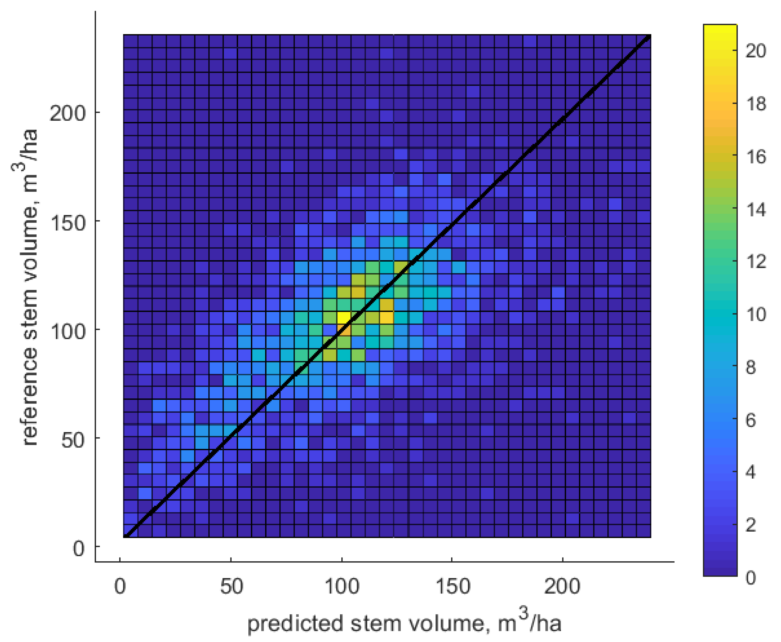
The scatterogram of the predictions using regression model and 78 features is shown in Figure 5. The correlation coefficient between the observed and predicted volume and is 0.62 when using the validation data set for prediction.
Our results compare favourably with accuracies reported in literature, not only compared to studies at C-band, but also at X- and L-band [45]. This is also the case when multitemporal and multipolarization SAR data were used. For example, in [41], the best result using multitemporal HV backscatter reached relative accuracy of 41.2%, co-polarization coherence from five scenes provided 35.8% and combination of all features resulted in 33.9% RMSE. These relative RMSEs were lower than in an earlier study [43] with semi-empirical model and multivariate regression (43%). Santoro et al. [42] used JERS-1 L-band data also for estimating stand level tree stem volume. The relative RMSEs varied with multi-temporal scenes from 25% (intensively managed homogeneous forests) to 51%.)
When estimating and comparing the prediction errors in regression or similar analyses, one should note that both the response variable y and the regressor variables x often include measurement errors or random errors, particularly in remote sensing-based approaches. These errors should be taken into account in estimating the total prediction errors and confidence intervals but are often omitted e.g., [47]. The prediction errors depend on the values of both y and x variables and the distributions of their errors. We reported here only the model errors. This question is discussed more in the Section 5.
5. Discussion
When assessing the usability of Sentinel-1 data for snow damage mapping, one should note that not all possibilities offered by Sentinel-1 data have been investigated in this study. For example SAR interferometry with Sentinel-1 provides interferometric data with 6-days temporal baseline that could be applicable for forest parameter estimation [42,48] in the boreal winter conditions.
It is however important to keep in mind that reference data in this study are of somewhat lower quality compared to ground-collected measurements, as well as there is a time discrepancy of several years. Thus, further research with multitemporal Sentinel-1 data and ground-measured reference data would be needed to further support these results.
Examples of other possible sources for uncertainties in this study were as follows: (1) The timing of the snow damage event was not accurate. Most damage happened during late December 2017 though, but some possibly earlier or later. (2) The reference data consisted of the cutting operations caused by snow damage and reported by the forestry operators. A larger area than just a damaged area is often cut. (3) The reference data did not include all damaged stands, only those in which a cutting operation was done by the early April 2018.
Further research questions for the forthcoming studies, in addition to the use of SAR interferometry, could be (1) what kind of observation period is needed, (2) what is minimum number of the scenes needed, (3) further analyses with the SAR features and analysis methods, and (4) whether it is possible to develop a robust method to localize the damage without reference data from the area in question. The first point can partly be answered by varying the number of scenes and the length of time-interval, and also, removing from the analysis those stands that were snow damaged after the scene period. The question (4) is demanding.
The effect of using training data with errors both in y and x variables on the validation results and on the confidence intervals of the predictions is a demanding question and should be the practice in these types of studies. In remote sensing-based approaches, the training data are often measured using sampling, e.g., at plot level or at stand level resulting in errors in y variable. Furthermore, x variables, remote sensing features, also include random errors. The total confidence interval of an individual estimate (here volume estimate) depends on the x-variables and also the y-variable estimate, in addition to their errors and the covariance of the errors. The proper prediction errors should take into account these errors but needs knowledge of the error distributions. We wanted not to go this far in the reported results but will address this important question in the future studies. One reason for leaving the total error budget for the forthcoming studies is that the volume estimation was a kind of side-topic in the current study. We reported only the average RMSEs based on the validation with the independent data. The stand level RMSE in the MS-NFI data depends also on the ground truth. The error range 30–40% represents an average of the errors in y variable. The total prediction errors and confidence intervals should be reported by the y-variable values or classes.
Overall, despite of the lacks in error estimating to the total prediction errors, the outcomes of the study encourage to continue the research efforts toward an operational system. The outcomes were well received by the forest authorities responsible for damage monitoring and sanitary cutting operations.
6. Conclusions and Outlook
We have studied the applicability of Sentinel-1 C-band SAR time series for a rapid localization of forest crown snow-load damage. There is a high practical need for this type of method to optimize forest management regimes and minimize economical losses. Three different methods were tested and some typical SAR features used in damage mapping. Of the methods tested, the SVM gave the highest overall accuracy (91%) and also the user accuracy while ik-NN gave the highest producer accuracy in localizing the stands damaged and cut due to a heave snow-load. SVM showed the highest overall performance based on these tests. However, in possible operational mapping tasks, several methods could be used. The accuracy was surprisingly high particularly when considering some lacks in the reference data. Not all damage was identified by the date of the field data acquisition wherefore some stands assumed non-damaged and picked up randomly for the training data may have been damaged.
The study is the first one to localize snow damage by means of time series of C-band SAR data. The outcomes encourage to continue the study towards an operational system. Possible further research questions and possibilities to decrease the uncertainties were listed.
On optimal operative method would be such that the severity of a damage could also be assessed, that is, in addition to the area, also the tree stem volume damaged and its economical value. This is a very demanding task due to the many types of damage and also due to the fact that a part of the broken stems can be used by forest industries or for other purposes. The first item towards the severity estimation is to investigate the capability of SAR time series in estimating growing stock volume. We tested two methods and a two lengths of the Sentinel-1 time series. The stand level volume of all species together and the volume of the main tree species (Scots pine) were estimated quite accurately. The relative root mean errors of the estimate of the all species together varied between 33% and 37% and that of Scots pine between 35% and 40%, depending on the method and on the number of the Sentinel-1 scenes. Assessment of the economical value of the losses caused by a damage would presume the assessments of the losses separately in saw timber and pulp wood, in addition to the total volume, because the stumpage price of saw timber is many times higher than that of the pulp wood. A priori information of the target, that is, the structure of the growing stock, as well a data bank of the damage types in different types of forests would help in assessments. L-band SAR data have also better capability to penetrate to forest and give more information on the stems than C-band SAR data. Overall, the results with C-band time series data are promising and make a good basis to develop also methods to estimate the volume of the growing stock and its change as well as the value of the economical losses.
Author Contributions
E.T. and J.P. designed the study; O.A. was responsible for data acquisition and pre-processing; E.T. and O.A. were primarily responsible for the method development; E.T. was responsible for reference data provision; and J.P. was involved in the method development. All authors participated in the interpretation of the results and associated discussions, as well as revising the manuscript.
Funding
The study has been funded by Bitcomp Oy, Jyväskylä, Finland, Aalto University, Espoo, Finland, and VTT Technical Research Centre of Finland.
Acknowledgments
Yrjö Niskanen, Finnish Forest Centre, provided the damage data and discussed the research questions. Three anonymous reviewers have provided detailed and constructive comments that improved the manuscript significantly. The authors sincerely thank all institutes and individuals that have supported the study.
Conflicts of Interest
The authors declare no conflict of interest.
Abbreviations
The following abbreviations are used in this manuscript:
| SAR | synthetic aperture radar |
| ESA | European Space Agency |
| SVM | support vector machine |
| LiDAR | light detection and ranging |
| k-NN | k Nearest Neighbours |
| ik-NN | improverd k Nearest Neighbours |
| RBF | radial basis function |
References
- Suvanto, S.; Henttonen, H.M.; Nöjd, P.; Mäkinen, H. Forest susceptibility to storm damage is affected by similar factors regardless of storm type: Comparison of thunder storms and autumn extra-tropical cyclones in Finland. For. Ecol. Manag. 2016, 381, 17–28. [Google Scholar] [CrossRef]
- Suvi Jylhänlehto, S. Metsäkeskus Kokosi Lumituhot Kartalle—Tykkytuhohakkuita Jopa Miljoona Mottia. Maaseudun Tulevaisuus, 2018. (in Finnish). Available online: https://bit.ly/2Hu6Bx1 (accessed on 12 February 2019).
- Torres, R.; Snoeij, P.; Geudtner, D.; Bibby, D.; Davidson, M.; Attema, E.; Potin, P.; Rommen, B.; Floury, N.; Brown, M.; et al. GMES Sentinel-1 mission. Remote Sens. Environ. 2012, 120, 9–24. [Google Scholar] [CrossRef]
- Vastaranta, M.; Korpela, I.; Uotila, A.; Hovi, A.; Holopainen, M. Area-Based Snow Damage Classification of Forest Canopies Using—Temporal LIDAR Data. ISPRS Int. Arch. Photogramm. Remote Sens. Spat. Inf. Sci. 2011, 3812, 169–173. [Google Scholar] [CrossRef]
- Honkavaara, E.; Litkey, P.; Nurminen, K. Automatic Storm Damage Detection in Forests Using High? Altitude Photogrammetric Imagery. Remote Sens. 2013, 5, 1405–1424. [Google Scholar] [CrossRef]
- Nelson, M.; Healey, S.; Moser, W.K.; Hansen, M. Combining satellite imagery with forest inventory data to assess damage severity following a major blowdown event in northern Minnesota, USA. Int. J. Remote Sens. 2009, 30, 5089–5108. [Google Scholar] [CrossRef]
- Einzmann, K.; Immitzer, M.; Böck, S.; Bauer, O.; Schmitt, A.; Atzberger, C. Windthrow Detection in European Forests with Very High-Resolution Optical Data. Forests 2017, 8, 21. [Google Scholar] [CrossRef]
- Joshi, N.; Mitchard, E.T.; Woo, N.; Torres, J.; Moll-Rocek, J.; Ehammer, A.; Collins, M.; Jepsen, M.R.; Fensholt, R. Mapping dynamics of deforestation and forest degradation in tropical forests using radar satellite data. Environ. Res. Lett. 2015, 10, 034014. [Google Scholar] [CrossRef]
- Thiele, A.; Boldt, M.; Hinz, S. Automated detection of storm damage in forest areas by analyzing TerraSAR-X data. In Proceedings of the 2012 IEEE International Geoscience and Remote Sensing Symposium, Munich, Germany, 22–27 July 2012; pp. 1672–1675. [Google Scholar] [CrossRef]
- Rosa, R.A.S.; Fernandes, D.; Nogueira, J.B.; Wimmer, C. Automatic change detection in multitemporal X- and P-band SAR images using Gram-Schmidt process. In Proceedings of the 2015 IEEE International Geoscience and Remote Sensing Symposium (IGARSS), Milan, Italy, 26–31 July 2015; pp. 2797–2800. [Google Scholar] [CrossRef]
- Antropov, O.; Rauste, Y.; Väänänen, A.; Mutanen, T.; Häme, T. Mapping forest disturbance using long time series of Sentinel-1 data: Case studies over boreal and tropical forests. In Proceedings of the 2016 IEEE International Geoscience and Remote Sensing Symposium (IGARSS), Beijing, China, 10–15 July 2016; pp. 3906–3909. [Google Scholar] [CrossRef]
- Santoro, M.; Pantze, A.; Fransson, J.E.S.; Dahlgren, J.; Persson, A. Nation-Wide Clear-Cut Mapping in Sweden Using ALOS PALSAR Strip Images. Remote Sens. 2012, 4, 1693–1715. [Google Scholar] [CrossRef]
- Rignot, E.J.M.; van Zyl, J.J. Change detection techniques for ERS-1 SAR data. IEEE Trans. Geosci. Remote Sens. 1993, 31, 896–906. [Google Scholar] [CrossRef]
- Quegan, S.; Toan, T.L.; Yu, J.J.; Ribbes, F.; Floury, N. Multitemporal ERS SAR analysis applied to forest mapping. IEEE Trans. Geosci. Remote Sens. 2000, 38, 741–753. [Google Scholar] [CrossRef]
- Ranson, K.J.; Kovacs, K.; Sun, G.; Kharuk, V.I. Disturbance recognition in the boreal forest using radar and Landsat-7. Can. J. Remote Sens. 2003, 29, 271–285. [Google Scholar] [CrossRef]
- Tanase, M.; Kennedy, R.; Aponte, C. Radar Burn Ratio for fire severity estimation at canopy level: An example for temperate forests. Remote Sens. Environ. 2015, 170, 14–31. [Google Scholar] [CrossRef]
- Pantze, A.; Santoro, M.; Fransson, J.E.S. Change detection of boreal forest using bi-temporal ALOS PALSAR backscatter data. Remote Sens. Environ. 2014, 155, 120–128. [Google Scholar] [CrossRef]
- Antropov, O.; Rauste, Y.; Astola, H.; Praks, J.; Häme, T.; Hallikainen, M.T. Land cover and soil type mapping from spaceborne PolSAR data at L-Band With probabilistic neural network. IEEE Trans. Geosci. Remote Sens. 2014, 52, 5256–5270. [Google Scholar] [CrossRef]
- Fransson, J.E.S.; Pantze, A.; Eriksson, L.E.B.; Soja, M.J.; Santoro, M. Mapping of wind-thrown forests using satellite SAR images. In Proceedings of the 2010 IEEE International Geoscience and Remote Sensing Symposium, Honolulu, HI, USA, 25–30 July 2010; pp. 1242–1245. [Google Scholar] [CrossRef]
- Eriksson, L.E.B.; Fransson, J.E.S.; Soja, M.J.; Santoro, M. Backscatter signatures of wind-thrown forest in satellite SAR images. In Proceedings of the 2012 IEEE International Geoscience and Remote Sensing Symposium, Munich, Germany, 22–27 July 2012; pp. 6435–6438. [Google Scholar] [CrossRef]
- Tanase, M.A.; Aponte, C.; Mermoz, S.; Bouvet, A.; Toan, T.L.; Heurich, M. Detection of windthrows and insect outbreaks by L-band SAR: A case study in the Bavarian Forest National Park. Remote Sens. Environ. 2018, 209, 700–711. [Google Scholar] [CrossRef]
- Rüetschi, M.; Small, D.; Waser, L.T. Rapid Detection of Windthrows Using Sentinel-1 C-Band SAR Data. Remote Sens. 2019, 11, 115. [Google Scholar] [CrossRef]
- Mákisara, K.; Katila, M.; Peräsaari, J.; Tomppo, E. The Multi-source National Forest Inventory of Finland—Methods and results 2013. Nat. Resour. Bioecon. Stud. 2016, 10, 215. [Google Scholar]
- Tomppo, E.; Halme, M. Using coarse scale forest variables as ancillary information and weighting of variables in k-NN estimation: A genetic algorithm approach. Remote Sens. Environ. 2004, 92, 1–20. [Google Scholar] [CrossRef]
- Tomppo, E.; Haakana, M.K.M.P.J. Multi-Source National Forest Inventory—Methods and Applications. Managing Forest Ecosystems; Springer: Dordrecht, The Netherlands, 2008. [Google Scholar]
- Tomppo, E.; Olsson, H.; Ståhl, G.; Nilsson, M.; Hagner, O.; Katila, M. Combining national forest inventory field plots and remote sensing data for forest databases. Remote Sens. Environ. 2008, 112, 1982–1999. [Google Scholar] [CrossRef]
- National Land Survey of Finland. Elevation Model 10 m. In Maps and Spatial Data; National Land Survey of Finland: Helsinki, Finland, 2018. [Google Scholar]
- Tomppo, E.O.; Gagliano, C.; Natale, F.D.; Katila, M.; McRoberts, R.E. Predicting categorical forest variables using an improved k-Nearest Neighbour estimator and Landsat imagery. Remote Sens. Environ. 2009, 113, 500–517. [Google Scholar] [CrossRef]
- Cortes, C.; Vapnik, V. Support-Vector Networks. Mach. Learn. 1995, 20, 273–297. [Google Scholar] [CrossRef]
- McRoberts, R.E. Post-classification approaches to estimating change in forest area using remotely sensed auxiliary data. Remote Sens. Environ. 2014, 151, 149–156. [Google Scholar] [CrossRef]
- Chirici, G.; Mura, M.; McInerney, D.; Py, N.; Tomppo, E.O.; Waser, L.T.; Travaglini, D.; McRoberts, R.E. A meta-analysis and review of the literature on the k-Nearest Neighbors technique for forestry applications that use remotely sensed data. Remote Sens. Environ. 2016, 176, 282–294. [Google Scholar] [CrossRef]
- Mountrakis, G.; Im, J.; Ogole, C. Support vector machines in remote sensing: A review. ISPRS J. Photogramm. Remote Sens. 2011, 66, 247–259. [Google Scholar] [CrossRef]
- Huang, C.; Davis, L.S.; Townshend, J.R.G. An assessment of support vector machines for land cover classification. Int. J. Remote Sens. 2002, 23, 725–749. [Google Scholar] [CrossRef]
- Camps-Valls, G.; Gomez-Chova, L.; Munoz-Mari, J.; Rojo-Alvarez, J.L.; Martinez-Ramon, M. Kernel-Based Framework for Multitemporal and Multisource Remote Sensing Data Classification and Change Detection. IEEE Trans. Geosci. Remote Sens. 2008, 46, 1822–1835. [Google Scholar] [CrossRef]
- Pal, M.; Mather, P.M. Support vector machines for classification in remote sensing. Int. J. Remote Sens. 2005, 26, 1007–1011. [Google Scholar] [CrossRef]
- Kuo, B.; Ho, H.; Li, C.; Hung, C.; Taur, J. A Kernel-Based Feature Selection Method for SVM With RBF Kernel for Hyperspectral Image Classification. IEEE J. Sel. Top. Appl. Earth Obs. Remote Sens. 2014, 7, 317–326. [Google Scholar] [CrossRef]
- Vapnik, V.N. The Nature of Statistical Learning Theory; Springer Inc.: New York, NY, USA, 1995. [Google Scholar]
- Tibshirani, R. Regression Shrinkage and Selection Via the Lasso. J. R. Stat. Soc. Ser. B 1994, 58, 267–288. [Google Scholar] [CrossRef]
- Kim, H.J.; Tomppo, E. Model-based prediction error uncertainty estimation for k-nn method. Remote Sens. Environ. 2006, 104, 257–263. [Google Scholar] [CrossRef]
- McRoberts, R.E.; Tomppo, E.O.; Finley, A.O.; Heikkinen, J. Estimating areal means and variances of forest attributes using the k-Nearest Neighbors technique and satellite imagery. Remote Sens. Environ. 2007, 111, 466–480. [Google Scholar] [CrossRef]
- Antropov, O.; Rauste, Y.; Häme, T.; Praks, J. Polarimetric ALOS PALSAR Time Series in Mapping Biomass of Boreal Forests. Remote Sens. 2017, 9, 999. [Google Scholar] [CrossRef]
- Santoro, M.; Eriksson, L.; Askne, J.; Schmullius, C. Assessment of stand-wise stem volume retrieval in boreal forest from JERS-1 L-band SAR backscatter. Int. J. Remote Sens. 2006, 27, 3425–3454. [Google Scholar] [CrossRef]
- Antropov, O.; Rauste, Y.; Ahola, H.; Hame, T. Stand-Level Stem Volume of Boreal Forests From Spaceborne SAR Imagery at L-Band. IEEE J. Sel. Top. Appl. Earth Obs. Remote Sens. 2013, 6, 35–44. [Google Scholar] [CrossRef]
- Kurvonen, L.; Pulliainen, J.; Hallikainen, M. Retrieval of biomass in boreal forests from multitemporal ERS-1 and JERS-1 SAR images. IEEE Trans. Geosci. Remote Sens. 1999, 37, 198–205. [Google Scholar] [CrossRef]
- Sinha, S.; Jeganathan, C.; Sharma, L.K.; Nathawat, M.S. A review of radar remote sensing for biomass estimation. Int. J. Environ. Sci. Technol. 2015, 12, 1779–1792. [Google Scholar] [CrossRef]
- Næsset, E. Airborne laser scanning as a method in operational forest inventory: Status of accuracy assessments accomplished in Scandinavia. Scand. J. For. Res. 2007, 22, 433–442. [Google Scholar] [CrossRef]
- Buonaccorsi, J.P. Prediction in the Presence of Measurement Error: General Discussion and an Example Predicting Defoliation. Biometrics 1995, 51, 562–1569. [Google Scholar] [CrossRef]
- Olesk, A.; Praks, J.; Antropov, O.; Zalite, K.; Arumae, T.; Voormansik, K. Interferometric SAR Coherence Models for Characterization of Hemiboreal Forests Using TanDEM-X Data. Remote Sens. 2016, 8, 700. [Google Scholar] [CrossRef]
Figure 1.
Location of the test site in Northern Finland, Kainuu county (left) and corresponding color-coded representation of Sentinel-1 scene (red corresponds to VV, green to VH and blue to VV-to-VH ratio).
Figure 1.
Location of the test site in Northern Finland, Kainuu county (left) and corresponding color-coded representation of Sentinel-1 scene (red corresponds to VV, green to VH and blue to VV-to-VH ratio).

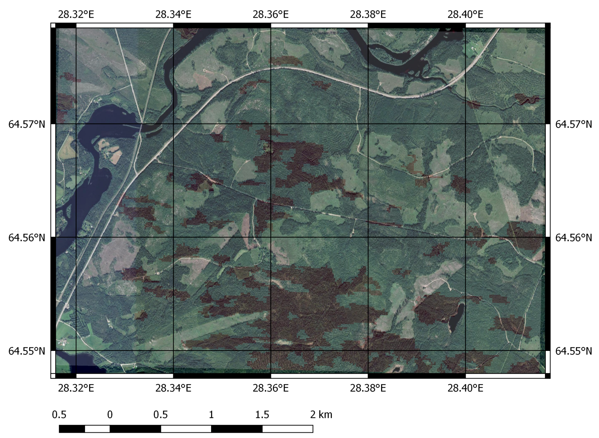
Figure 2.
An example of a colour composition of Sentinel-1 image (scene no 7). Highlighted rectangle is used in illustrating snow-damage map further.
Figure 2.
An example of a colour composition of Sentinel-1 image (scene no 7). Highlighted rectangle is used in illustrating snow-damage map further.

Figure 3.
The flowchart of the study.

Figure 4.
An example of snow-load damage map (brown) displayed on a Google Earth scene ©Google Earth. The area size is 4.8 km by 3.4 km.
Figure 4.
An example of snow-load damage map (brown) displayed on a Google Earth scene ©Google Earth. The area size is 4.8 km by 3.4 km.

Figure 5.
Reference stand level growing stock volume versus predicted growing stock volume based on regression analysis (m/ha).
Figure 5.
Reference stand level growing stock volume versus predicted growing stock volume based on regression analysis (m/ha).


Table 1.
List of Sentinel-1 scenes used in the study.
| Image | Date | Mode | Polarization |
|---|---|---|---|
| 1 | 12 November 2017 | IW | VV, VH |
| 2 | 24 November 2017 | IW | VV, VH |
| 3 | 6 December 2017 | IW | VV, VH |
| 4 | 18 December 2017 | IW | VV, VH |
| 5 | 30 December 2017 | IW | VV, VH |
| 6 | 11 January 2018 | IW | VV, VH |
| 7 | 23 January 2018 | IW | VV, VH |
| 8 | 4 February 2018 | IW | VV, VH |
| 9 | 16 February 2018 | IW | VV, VH |
| 10 | 28 February 2018 | IW | VV, VH |
| 11 | 12 March 2018 | IW | VV, VH |
| 12 | 24 March 2018 | IW | VV, VH |
Table 2.
Stand level accuracy metrics with separate validation data.
| Method | Overall Accuracy | User Accuracy | Producer Accuracy | ||
|---|---|---|---|---|---|
| Damage | Non-Damage | Damage | Non-Damage | ||
| SVM | 0.91 | 0.90 | 0.91 | 0.72 | 0.97 |
| ik-NN | 0.75 | 0.72 | 0.78 | 0.80 | 0.69 |
| Logistic regression | 0.71 | 0.69 | 0.73 | 0.76 | 0.67 |
Table 3.
Stand level accuracy metrics with ik-NN using separate validation data for stands with an area of at least 1 hectare.
Table 3.
Stand level accuracy metrics with ik-NN using separate validation data for stands with an area of at least 1 hectare.
| Method | Overall Accuracy | User Accuracy | Producer Accuracy | ||
|---|---|---|---|---|---|
| Damage | Non-Damage | Damage | Non-Damage | ||
| ik-NN with stands | |||||
| area ≥ 1 ha | 0.79 | 0.77 | 0.82 | 0.86 | 0.71 |
Table 4.
Average volume estimate in the test sites, mean deviations and the relative root mean square errors in the validation data sets by tree species groups, 1867 stand in the training data set, 1867 stands in the validation data set.
Table 4.
Average volume estimate in the test sites, mean deviations and the relative root mean square errors in the validation data sets by tree species groups, 1867 stand in the training data set, 1867 stands in the validation data set.
| Tree Species | Estimate (m/ha) | Mean Deviation (m/ha) | RMSE (%) |
|---|---|---|---|
| ik-NN, 12 features | |||
| All species | 100.7 | 0.25 | 36.3 |
| Pine | 61.1 | 1.26 | 36.8 |
| Spruce | 20.1 | −0.70 | 101.2 |
| Birch sp | 17.6 | −0.22 | 59.5 |
| Other br. leaved | 1.9 | −0.09 | 166.9 |
| Regression analysis, 12 features | |||
| All species | 101.9 | 1.43 | 37.0 |
| Pine | 59.3 | −0.58 | 40.1 |
| Spruce | 30.3 | 9.56 | 70.7 |
| Birch sp | 19.2 | 1.37 | 55.9 |
| Other br. leaved | 5.7 | 3.76 | 60.1 |
| ik-NN, all 78 features | |||
| All species | 100.4 | −0.01 | 34.1 |
| Pine | 61.3 | 1.46 | 34.7 |
| Spruce | 19.9 | −0.82 | 97.0 |
| Birch sp | 17.3 | −0.47 | 59.8 |
| Other br. leaved | 1.8 | −0.18 | 171.6 |
| Regression analysis, all 78 features | |||
| All species | 101.3 | 0.88 | 32.7 |
| Pine | 59.5 | −0.43 | 36.4 |
| Spruce | 27.4 | 6.69 | 69.0 |
| Birch sp | 19.1 | 1.32 | 54.9 |
| Other br. leaved | 5.5 | 3.51 | 61.7 |
© 2019 by the authors. Licensee MDPI, Basel, Switzerland. This article is an open access article distributed under the terms and conditions of the Creative Commons Attribution (CC BY) license (http://creativecommons.org/licenses/by/4.0/).
Share and Cite
MDPI and ACS Style
Tomppo, E.; Antropov, O.; Praks, J. Boreal Forest Snow Damage Mapping Using Multi-Temporal Sentinel-1 Data. Remote Sens. 2019, 11, 384. https://0-doi-org.brum.beds.ac.uk/10.3390/rs11040384
AMA Style
Tomppo E, Antropov O, Praks J. Boreal Forest Snow Damage Mapping Using Multi-Temporal Sentinel-1 Data. Remote Sensing. 2019; 11(4):384. https://0-doi-org.brum.beds.ac.uk/10.3390/rs11040384
Chicago/Turabian StyleTomppo, Erkki, Oleg Antropov, and Jaan Praks. 2019. "Boreal Forest Snow Damage Mapping Using Multi-Temporal Sentinel-1 Data" Remote Sensing 11, no. 4: 384. https://0-doi-org.brum.beds.ac.uk/10.3390/rs11040384
Note that from the first issue of 2016, this journal uses article numbers instead of page numbers. See further details here.