Article

S-RVoG Model Inversion Based on Time-Frequency Optimization for P-Band Polarimetric SAR Interferometry

1
National Key Lab of Microwave Imaging Technology, Institute of Electronics, Chinese Academy of Sciences, Beijing 100190, China
2
School of Electronic, Electrical and Communication Engineering, University of Chinese Academy of Sciences, Beijing 100049, China
3
School of Optical-Electrical and Computer Engineering, University of Shanghai for Science and Technology, Shanghai 200093, China
*
Author to whom correspondence should be addressed.
Submission received: 7 March 2019 / Revised: 18 April 2019 / Accepted: 23 April 2019 / Published: 1 May 2019
(This article belongs to the Special Issue Remote Sensing of Boreal Forests)

Abstract

:
This paper investigates the potential of the time-frequency optimization on the basis of the sublook decomposition for forest height estimation. The optimization is deemed to be capable of extracting a relatively accurate volume contribution when P-band polarimetric interferometric synthetic aperture radar (Pol-InSAR) systems are adopted to observe forest-covered areas. The highest and the lowest phase centers acquired by the time-frequency optimization modify the conventional three-stage inversion process. This paper presents, for the first time, a performance assessment of the time-frequency optimization on P-band Pol-InSAR data over boreal forests. Simultaneously, to alleviate the model inversion errors caused by topographic fluctuations, forest height is estimated based on the sloped Random Volume over Ground (S-RVoG) model in which the incidence angle is corrected with the terrain slope. The E-SAR P-band Pol-InSAR data acquired during the BIOSAR 2008 campaign in Northern Sweden is utilized to evaluate the performance of the proposed method. From the results of the forest height estimation preprocessed with time-frequency optimization, the root mean square error (RMSE) of Random Volume over Ground (RVoG) and S-RVoG model on negative slope are 5.09 m and 4.71 m, respectively. It is concluded that the time-frequency processing and negative terrain slope compensation improve the inversion performance by 41 . 49 % and 11 . 96 % , respectively.

1. Introduction

On account of the significant penetration of P-band polarimetric interferometric synthetic aperture radar (Pol-InSAR) systems, all polarimetric channels contain a non-ignorable ground contribution [1,2,3,4,5], generally leading to an underestimation of forest height in view of the Random Volume over Ground (RVoG) model [3,6]. So far, the RVoG model depicting the forest vertical backscatter profile with an exponential function has been widely taken advantage of in forest height estimation [7,8,9,10,11,12,13,14,15,16,17,18,19,20]. Moroever, when referring to temporal decorrelation [21,22,23,24,25], canopy filling [12,26] and terrain fluctuations [6,27,28,29,30,31,32], some modified models were proposed to complement the RVoG model. Under the circumstance of the Quad-pol single-baseline observation, the forest height estimation based on the RVoG model is a six-dimensional parameter optimization problem [1,3,5,10,12]. In order to retrieve the forest height with Quad-pol single-baseline data, the null ground-to-volume ratio (NGVR) hypothesis is frequently adopted to derive a unique solution from the RVoG inversion equation [3,12]. Specifically, the NGVR hypothesis indicates that the ground-to-volume ratio (GVR) of at least one polarimetric channel is sufficiently small, usually less than −10 dB [12]. In view of the RVoG model, the three-stage [12] inversion process applying single-baseline data has been widely implemented for forest height acquisition [15,31,33,34]. That is a geometric inversion method that requires fitting the estimated coherences of various polarimetric channels to obtain the coherence line on the complex plane. Thus, the ground level and canopy contributions deemed to be on the coherence line can then be achieved. Ultimately, the forest height is extracted from the estimated volume coherence by the look-up table method.
Previous work has manifested that the forest height estimation based on RVoG model presents a relatively high accuracy at L-band Pol-InSAR observations over boreal forests [6]. However, due to the strong penetration of P-band and the sparsity of boreal forest, the traditional three-stage method based on the RVoG model is no longer effective, specifically, leading to a serious underestimation. That is because the NGVR assumption is invalid under this circumstance. Up to now, two main strategies have been adopted to ameliorate the underestimation [3,35]. The first strategy is to increase the observation space with multi-baseline data [3,26,36,37,38]. Nevertheless, it brings about a high complexity of data acquisition and model inversion. The second strategy is to fix the extinction coefficient so that the single-baseline inversion is still feasible [1], yet the inversion performance is heavily dependent on the choice of the fixed extinction coefficient. To overcome the above limitations, the time-frequency optimization was developed as a method independent of the above two strategies, allowing a separation of the canopy and ground contributions with single-baseline Pol-InSAR data [2]. The sublook decomposition is operated in the azimuth direction on the Pauli and lexicographic base polarimetric channels. Then, the polarimetric channels corresponding to the highest and the lowest phase centers are assumed to be related to the canopy and ground contributions, respectively. Since it exclusively takes into account the polarimetric channels consistent with the highest and lowest phase centers, with different polarimetric coherences not necessarily located on a straight line on the complex plane, this method fundamentally derives from the Oriented Volume over Ground (OVoG) [9,39,40,41] model. The ground coherence is not constrained to equal one, as the lowest phase estimated by time-frequency optimization is directly regarded as being related to the ground level contribution. This processing yields a highly accurate forest height inversion for the RAMSES data [2].
Topographic fluctuations have been manifested to be one of the significant factors affecting the performance of the model-based Pol-InSAR inversion [6,27,28,29,30,31,32]. Specifically, the positive terrain slope causes an overestimation of the forest height, while the negative terrain slope causes an underestimation of the forest height [6,29,30,32]. For the purpose of eliminating the influence of terrain, the sloped Random Volume over Ground (S-RVoG) model was proposed by introducing the parameter of range terrain slope into the RVoG model [29]. With the addition of the model parameters, the multi-baseline optimization emerges as a direct inversion idea. Yet, when single-baseline optimization is still being implemented, prior terrain information is introduced to gain the terrain slope, which is then compensated into the RVoG model.
With the aim of obtaining a relatively precise volume coherence and simultaneously retaining the advantages of the single-baseline for inversion efficiency, this paper took advantage of the time-frequency optimization to separate ground and canopy contributions. The three-stage process is then modified with these two optimized coherences. Considering the influence of topographic fluctuations on forest height estimation, the S-RVoG model was adopted to improve the forest height inversion accuracy. The structure of this paper proceeds as follows. Section 2 presents the principle of the time-frequency optimization, while Section 3 introduces the S-RVoG model and illustrates the overall framework of model inversion. Afterwards, the verification of the real E-SAR data is presented in Section 4. Finally, Section 5 discusses and Section 6 concludes.

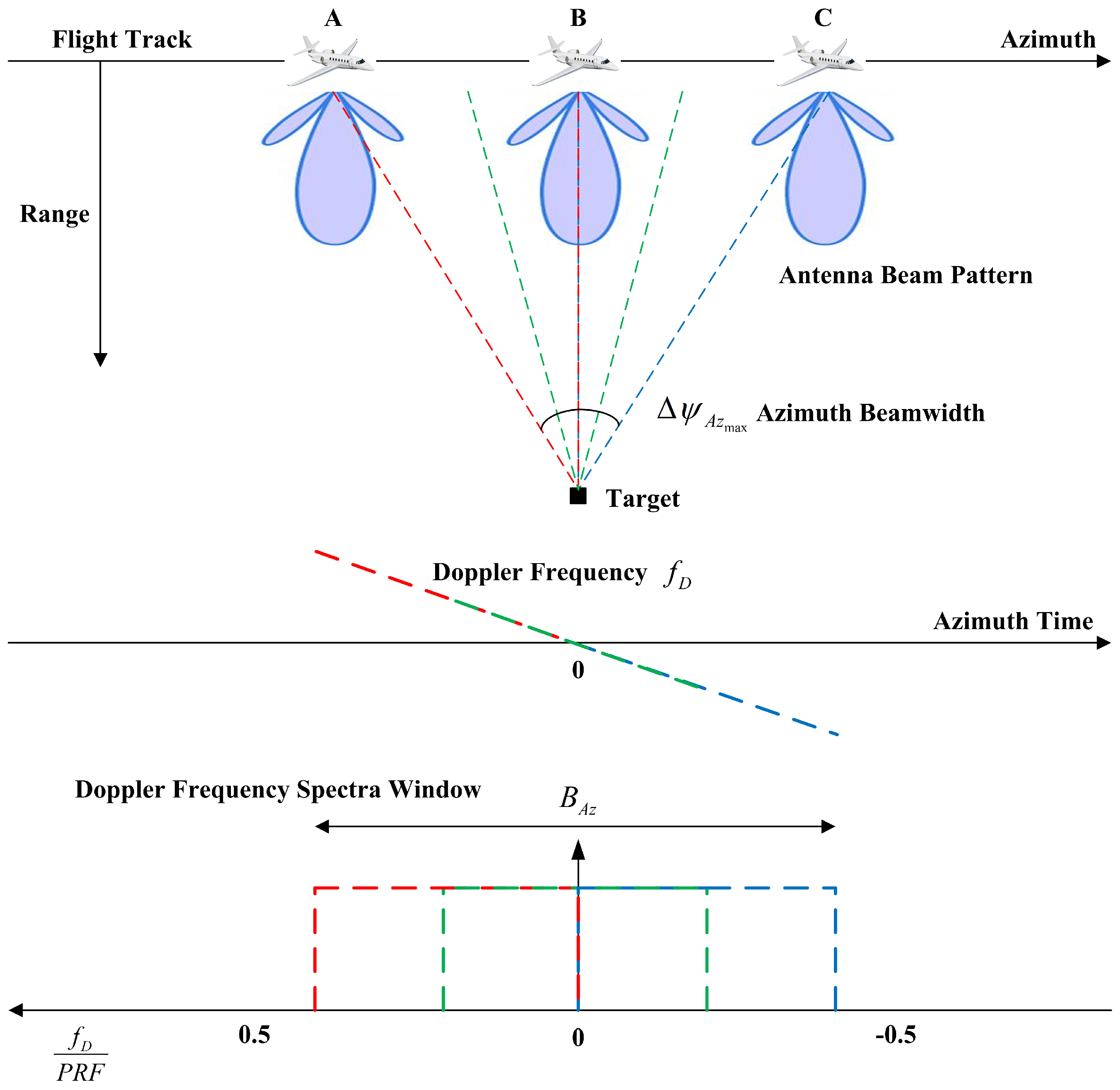
2. Time-Frequency Optimization Based on Sublook Decomposition

As mentioned earlier, to extract a relatively accurate volume coherence and to study the potential of the single-baseline configuration on P-band Pol-InSAR model inversion, the time-frequency optimization was proposed [2], which is based on synthetic aperture decomposition and Doppler filtering. This section will describe the principle and implementation of time-frequency optimization.
To improve the azimuth resolution, synthetic aperture radar (SAR) synthesizes a narrow beamwidth by time accumulation. The path that the sensor passes throughout this time is referred to as synthetic aperture length. During the synthetic aperture time, the Doppler history allows the azimuth signal to be treated as a chirp function, which is independent of the emitted signal. Therefore, as with signal processing in range, the azimuth focusing of the target imaging is also achieved by impulsion-compression. The top and center diagrams in Figure 1 indicate the synthetic aperture and Doppler history, respectively [42]. The synthetic aperture length pinpoints the actual antenna beamwidth, i.e., the scope of observation angle. In other words, the Doppler history is one-to-one with the radar observation angle. Therefore, the radar signal interrelating with the designated observation angle can be selected by filtering of Doppler spectra in the azimuth frequency-domain. Since diverse observation angles associate with diverse scattering characteristics [43,44,45], this time-frequency analysis can be utilized to separate the positions of various scattering centers [2,46].
The Doppler frequency [42] in Figure 1 can be expressed as a function of sensor speed v, radar wavelength λ , and observation angle θ s q
f D = 2 v sin θ s q λ
Since the Doppler frequency is proportional to the radial velocity of the target relative to the sensor, the absolute value of the Doppler frequency decreases first and then increases in the Doppler history. Furthermore, the Doppler frequency is positive when radar is approaching target, while presenting negative when the radar is moving away from the target. Therefore, the slope of the Doppler frequency versus time proves to be negative. The Doppler bandwidth [42] of the target is expressed as
B A z = 2 v cos θ s q c λ Δ ψ A z max
where θ s q c is the observation angle when the antenna beam center illuminates the target and Δ ψ A z max represents the 3-dB radar beamwidth. To fulfill the requirements of Nyquist sampling law, the bandwidth presented in Equation (2) determines the lower limit of the pulse-repetition frequency (PRF), i.e., P R F B A z . When PRF is greater than bandwidth, the normalized Doppler frequency spectra is specified in the bottom diagram of Figure 1 [42].
Marked with three different colors in Figure 1, the Doppler spectra is evenly divided into three parts through spectral filtering, overlapping each other by 50%. In accordance with Equation (1), the antenna patterns and observation angles corresponding to the three-segment spectra are also presented in Figure 1. Thus, the complete synthetic aperture is decomposed into three sublooks. Since a forest characterized by contrasted vegetation-density areas appears to have different scattering characteristics with various observation angles, the backscattered signal consistent with a specific observation angle allows to separate canopy and ground contributions, represented as high-density and low-density regions, respectively [2]. In the time-frequency analysis, the Doppler bandwidth scope is selected from the range-Doppler domain signal obtained by an azimuth Fourier transform, and then the sublook signal related to a specific observation angle is acquired employing an azimuth inverse Fourier transform. Since GVR varies with the observation angle for a given polarimetric channel [2], the separation of forest scattering centers is achieved by digging into the coherences of different sublooks. To sum up, the time-frequency optimization has the ability to independently extract backscattered signals at different observation angles, which means that it is possible to acquire a more accurate volume contribution. Therefore, this paper utilizes the optimization to improve the single-baseline P-band Pol-InSAR model inversion.

3. Model-Based Pol-InSAR Inversion

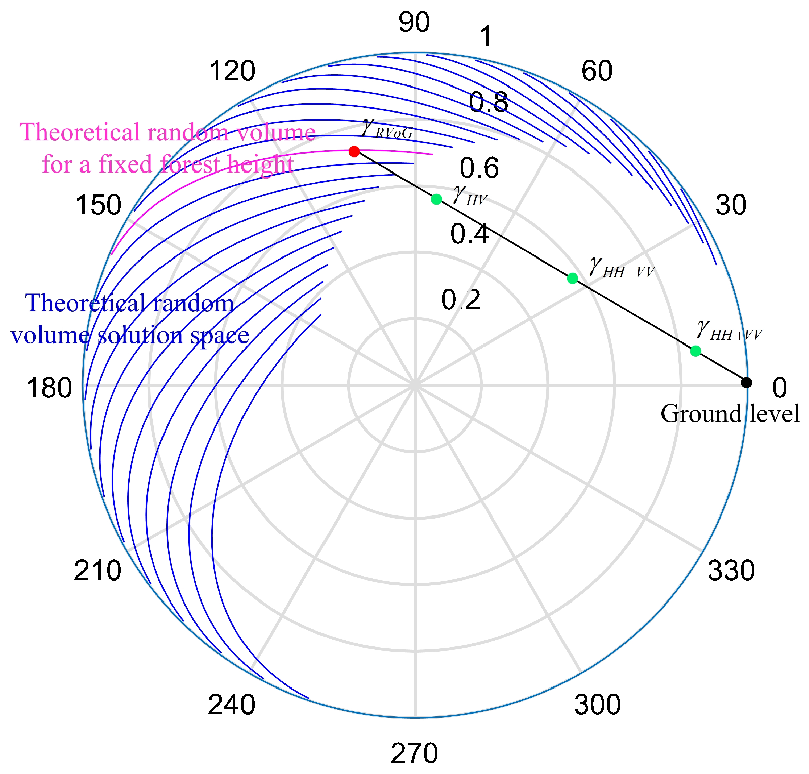
3.1. RVoG Model and Three-Stage Inversion Process

In the light of the assumption of the Volume over Ground [10,12] model, i.e., volume and ground contributions S v and S g , the interferometric coherence between the master and slave antennas S m and S s for a given polarimetric state ω is derived as follows:
γ ω = S m ω S s ω S m ω S m ω S s ω S s ω = S g m ω + S v m ω S g s ω + S v s ω S g m ω + S v m ω S g m ω + S v m ω S g s ω + S v s ω S g s ω + S v s ω = S g m ω S g s ω + S v m ω S v s ω S g ω 2 + S v ω 2 = S g m ω S g s ω S g ω 2 S g ω 2 S v ω 2 + S v m ω S v s ω S v ω 2 S g ω 2 S v ω 2 + 1 = e j ϕ 0 γ g μ ω + γ v μ ω + 1
where the subscripts m and s represent the master and slave antennas, respectively; * indicates the conjugate operation;   means the expectation; and ϕ 0 , γ g , μ ω , and γ v denote the ground interferometric phase, ground coherence, GVR, and volume coherence, respectively. Notice that, in Equation (3), the ground and volume contributions are recognized as irrelevant. Interferometric coherence can be altered to the following form [10,12]
γ ω = e j ϕ 0 γ v + L γ g γ v L ω = μ ω 1 + μ ω 0 L ω < 1 0 μ ω < +
In general, ground coherence is assumed to be one, i.e., γ g = 1 . It is concluded from Equation (4) that, for a given polarimetric state ω , the ground coherence γ g , interferometric coherence e j ϕ 0 γ ω , and volume coherence γ v are distributed on a straight line on the complex plane.
The RVoG [10,12] model adopting an exponential function to characterize the forest vertical backscatter profile deems that the volume coherence does not hinge on the polarimetric state, i.e., the assumption of random volume. On the basis of that assumption, the volume coherence with a forest height h v is represented as follows:
γ R V o G = 0 h v e 2 σ z cos θ e j k z z d z 0 h v e 2 σ z cos θ d z
where σ and θ denote, respectively, the mean extinction coefficient and the radar incidence angle. The interferometric vertical wavenumber k z depends on the wavelength λ , incidence angle θ , and its difference between the master and slave antennas Δ θ
k z = 4 π λ sin θ Δ θ
As is shown in Figure 2, since γ R V o G is independent of the polarimetric state, when the GVR varies, all the homologous interferometric coherences calculated in light of Equation (4) move on a straight line on the complex plane. In view of that geometric characteristic, the single-baseline Pol-InSAR inversion is divided into three stages [12]:
(1)
Coherence line fit: According to the linear distribution prediction of the coherences in Equation (4) or Figure 2, the coherence line can be achieved by fitting the coherences of different polarimetric channels.
(2)
Ground interferometric phase estimation: Similarly, according to Equation (4) or Figure 2, the ground interferometric phase corresponds to one of the two intersections of the coherence line with the unit circle. The criteria of judging the true ground phase is as follows
ϕ 0 = ϕ 0 1 , e j ϕ 0 1 γ H H + V V < e j ϕ 0 1 γ H V ϕ 0 2 , e l s e
where ϕ 0 1 and ϕ 0 2 indicate the two intersections of the coherence line with the unit circle. Equation (7) is based on the rank order of the polarimetric phase center positions, i.e., the HH+VV channel has a higher GVR than the HV channel, as shown in Figure 2. Since the phase diversity [47] can achieve a maximum phase separation, the PDHigh and PDLow channels can replace the HV and HH+VV channels in Equation (7).
(3)
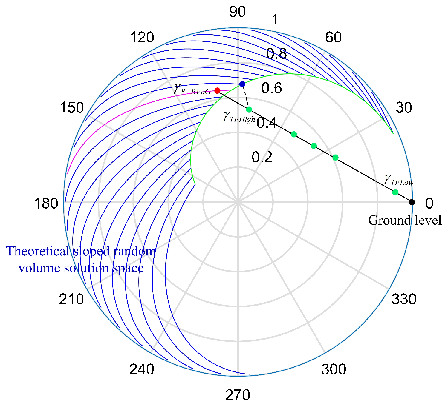
Forest height estimation: Assuming that the GVR of a polarimetric channel (such as the PDHigh channel) is sufficiently low, in accordance with Equation (4), the volume coherence can be expressed as e j ϕ 0 γ P D H i g h , and then the forest height is extracted by a two-dimensional look-up table (namely, the theoretical random volume solution space in Figure 2) set up in the light of Equation (5)
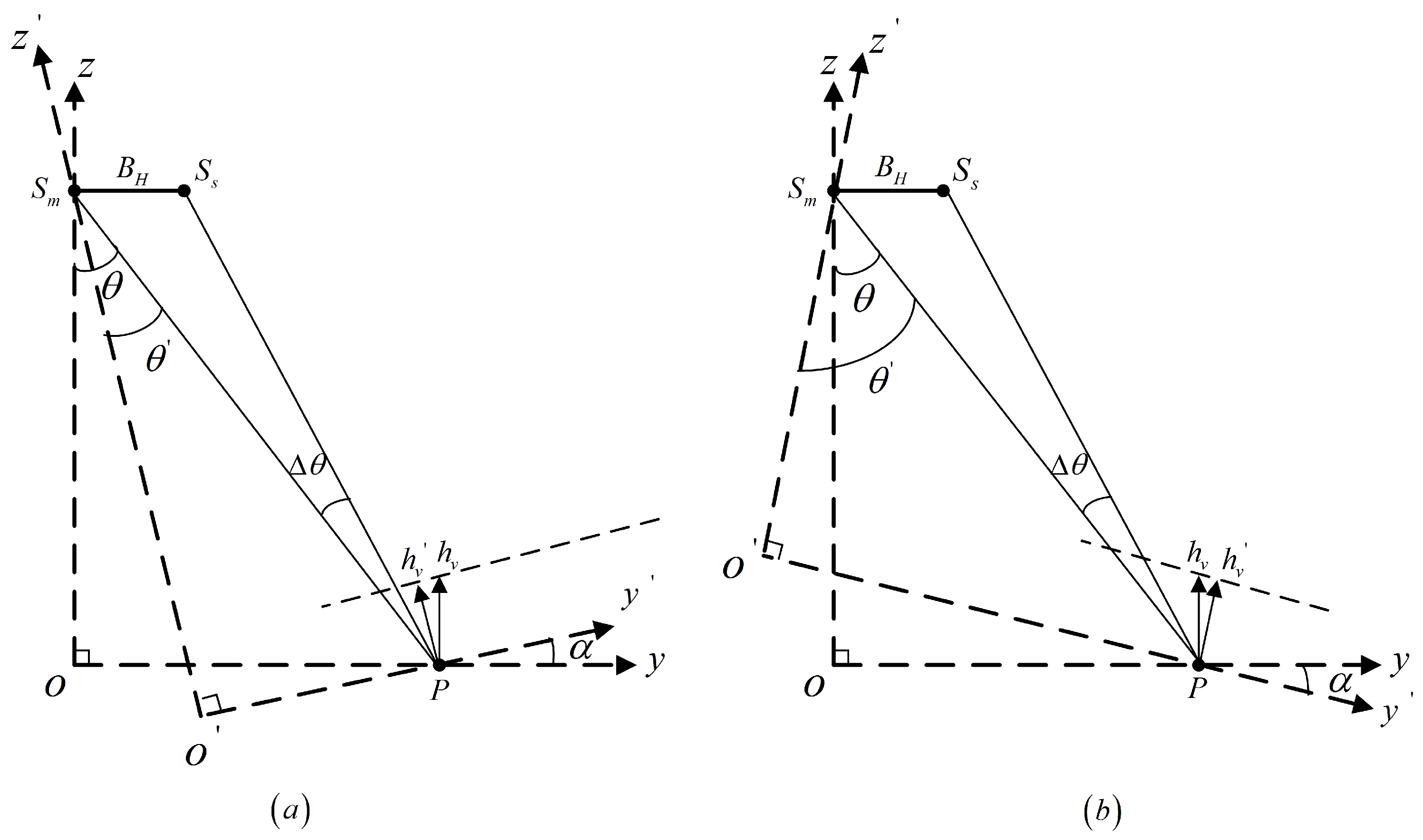
h ^ v = A r g min h v , σ e j ϕ 0 γ P D H i g h γ R V o G h v , σ

3.2. S-RVoG Model

Since the underlying topography over the forest area commonly takes on certain fluctuations, the forest height inversion on the basis of the traditional RVoG model under the flat ground hypothesis reckons to be susceptible to the terrain slope [6,27,28,29,30,31,32]. Accordingly, it is indispensable to incorporate the influence of the terrain slope into the forest height estimation. As shown in Figure 3, the terrain slope that tilted toward the radar called positive slope (see Figure 3a) decreases θ , whereas the slope that tilted away from the radar called negative slope (see Figure 3b) increases θ [30]. For reducing the complexity of inversion in consideration of the topography, the coordinate system is modified according to the terrain slope [29], denoted with y o z in Figure 3. In the corrected coordinate system y o z , the three-stage method is continuously effective for forest height inversion. Neglecting the influence of azimuth, the terrain slope α is achieved by the following equation [30]
α = tan 1 Δ H P S r g sin θ + Δ H tan θ
where Δ H calculated from the measured DEM is the altitude difference between two consecutive slant range samples and P S r g represents the homologous slant range distance. In Figure 3, the terrain slope α corresponding to a positive slope takes a positive value, while that corresponding to a negative slope takes a negative value. Thus, the local incidence angle corrected by α in the corrected coordinate system y o z is then rewritten as
θ = θ α
Since the local incidence angle is corrected by the terrain slope, interferometric vertical wavenumber k z also demands to be adjusted accordingly, while Δ θ remains unchanged before and after the coordinate system correction. Thus, the corrected vertical wavenumber can be expressed as
k z = 4 π λ sin θ Δ θ
Equations (5) and (6) present that θ and k z in volume coherence are directly dependent on the change in incidence angle. Therefore, in the corrected coordinate system y o z , the homologous volume coherence on account of the S-RVoG model requires an adjustment according as Equations (10) and (11), as shown in the following formula
γ S R V o G = 0 h v e 2 σ z cos θ e j k z z d z 0 h v e 2 σ z cos θ d z
where h v indicates the forest height in coordinate system y o z . It is concluded from Equations (10)–(12) that the positive slope increases k z , resulting in a decrease in the volume coherence, while the negative slope produces an opposite effect [30,32]. The essence of the volume coherence represented by Equation (12) is a process in which the accumulation of phase changes caused by k z is normalized. It manifests that when k z is equal to zero, namely the phase remains at zero, the volume coherence calculated in accordance with Equation (12) is identically equal to one. Under the circumstance, the calculation of volume coherence is independent of θ . The volume coherence reaches the maximum value at this time. When k z is greater than zero, the local incidence angle θ will also have an impact on the volume coherence. However, from Equation (12), θ has less effect than that of k z on the volume coherence. Consequently, as k z becomes larger, the volume coherence becomes smaller [30].
Since y o z is projected from y o z , the forest height estimation h v and h v in the two coordinate systems equally have a projection relationship, as shown in Figure 3. Hence, h v perpendicular to the horizon is obtained by performing an inverse projection operation on h v . The pertinent expression is as follows
h v = h v cos α
In addition, as can be seen from Figure 3, the relative extinction path has also changed in the corrected coordinate system, which directly affects the GVR. Therefore, Equation (4) is adjusted to the following form
γ ω = e j ϕ 0 γ v + L γ g γ v L ω = μ ω 1 + μ ω 0 L ω < 1 0 μ ω < +
where the superscript represents the parameters in the corrected coordinate system.
The concrete effect of the terrain slope on the volume coherence is shown in Figure 4. Compared with the random volume solution space in Figure 2, the volume coherence decreases on a positive terrain slope (see Figure 4a) while increases on a negative terrain slope (see Figure 4b), manifesting a consistence with the previous theoretical analysis. The pink and green curves represent γ S R V o G and γ R V o G for the same forest height, respectively. The findings reveal that, with the random volume solution space inversion, the positive terrain slope will cause an overestimation (see Figure 4a), whereas the negative terrain slope will cause an underestimation (see Figure 4b). Figure 4 presents the result after the projection relationship expressed by Equation (13) has been merged into the volume coherence calculated in line with Equation (12).

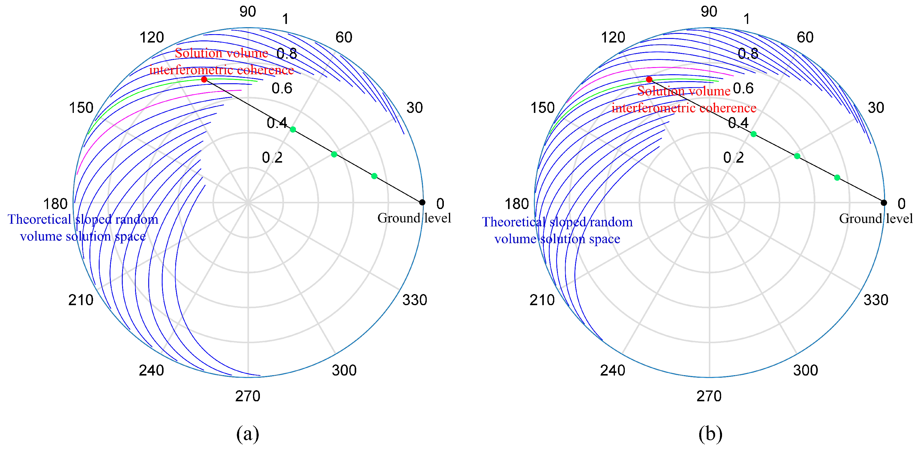
3.3. S-RVoG Model Inversion Based on Time-Frequency Optimization

Techniques such as polarimetric synthesis and coherence optimization [10,47] select different scattering centers from the scattering mechanism dimension, while time-frequency optimization separates phase centers from the observation angle dimension. For the purpose of achieving a maximum separation of the vertical phase center, in this paper, the time-frequency optimization is adopted to perform sublook decomposition imaging and then the highest (TFHigh) and lowest (TFLow) phase centers can be derived from the complex coherences of the selected polarimetric channels, which are estimated separately for each sublook image pair. To mitigate the effects of temporal decorrelation and noise, phase diversity [47] and magnitude diversity [10] optimizations are employed to pick the polarimetric channels for coherences estimation [48]. In regard to three-stage method, the polarimetric channel with a sufficiently small GVR [12] is pinpointed to estimate the volume coherence. Since the combination of the time-frequency analysis and coherence optimization can fulfill an effective separation of the scattering centers, it is reasonable to assume that a TFHigh channel corresponds to a relatively small GVR.
The S-RVoG inversion process is shown in Figure 5, in which γ T F H igh is presumed to be close enough to the real volume coherence [2]. Possibly, there is still some distance between γ T F H igh and the real volume coherence. The green curve indicates the theoretical sloped random volume for 0 dB/m extinction, namely the boundary of the solution space. When γ T F H igh does not fall into the solution space, the minimum Euclidean distance criterion referenced in the look-up table method provides a predicted volume coherence on the zero extinction curve which is represented in the blue dot in Figure 5. After preprocessing the data with the time-frequency optimization, the inversion process of the S-RVoG model is as follows. It should be noted that the process is still rooted on the framework of the traditional three-stage method.
(1)
Coherence line fit: This stage is consistent with the traditional three-stage approach. The total least squares method is adopted to fit the coherence line. γ T F H igh and γ T F L ow will take part in the fitting of the coherence line, further suppressing the effects of temporal decorrelation and noise.
(2)
Ground interferometric phase estimation: The ground interferometric phase is still acquired by one of the intersections of the coherence line and the unit circle, yet the criteria for selecting the real ground interferometric phase is adjusted
ϕ 0 = ϕ 0 1 , e j ϕ 0 1 γ T F L o w < e j ϕ 0 1 γ T F H i g h ϕ 0 2 , e l s e
(3)
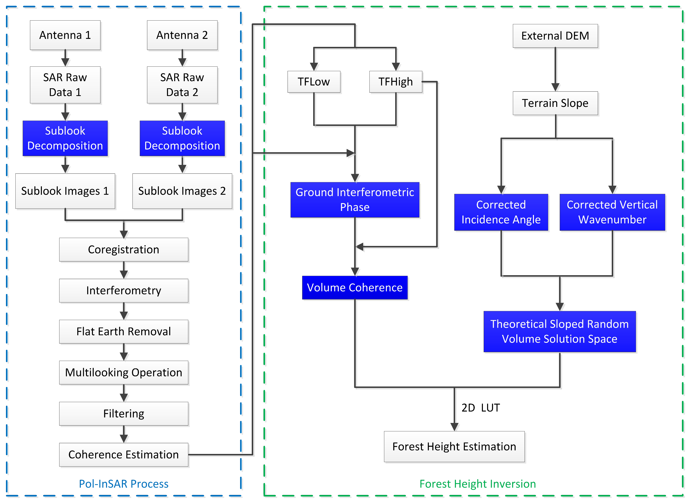
Forest height estimation: Since the GVR related to γ T F H igh is reckoned to be sufficiently small, that is, homologous L in Equation (14) is approximately equal to zero, the volume coherence is expressed as e j ϕ 0 γ T F H i g h . Therefore, the forest height is estimated from a two-dimensional look-up table which is generated in the light of Equation (12) on the basis of the minimum Euclidean distance criterion
h ^ v = A r g min h v , σ e j ϕ 0 γ T F H i g h γ S R V o G h v , σ h ^ v = h ^ v cos α
where h ^ v denotes the estimator of h v . Figure 6 portrays the flowchart of forest height inversion based on the time-frequency optimization reckoning terrain compensation. The blue block diagrams represent the key processing steps in this paper.

4. Forest Height Estimation Using P-Band E-SAR Data

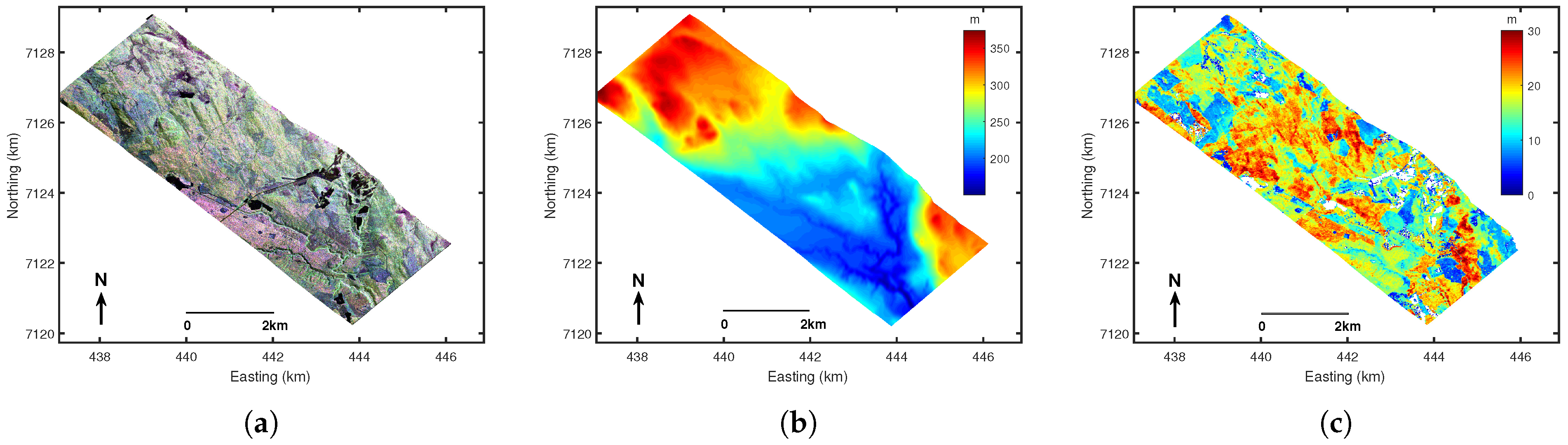
4.1. Test Site and E-SAR Data Description

This paper performs a method validation relying on the European Space Agency (ESA) BIOSAR 2008 data [6] acquired by the German Aerospace Center (DLR) E-SAR system in Krycklan catchment, Northern Sweden. The test site is mainly covered by boreal forest that is primarily between 0–30 m in height. The data set contains the lidar-derived forest height, which is applied to evaluate the performance of the inversion method. In addition, the measured topography elevation of the experimental area is utilized in this paper to generate terrain slope and to compensate for the inversion errors caused by topographic fluctuations. Figure 7 presents a pauli–basis composite map, measured DEM, and lidar-derived forest height of the test site. Table 1 shows the single-baseline data information researched in this paper.

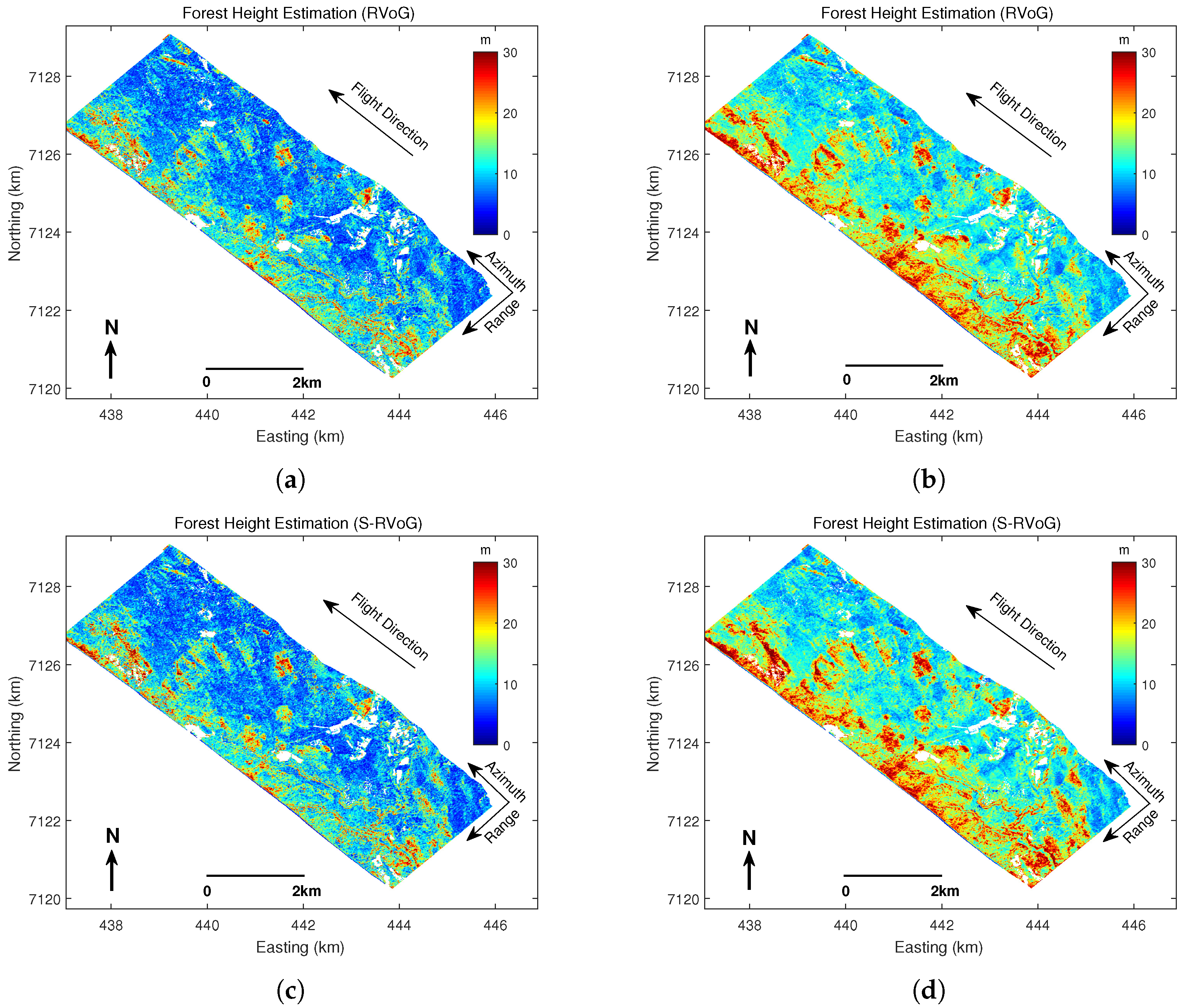
4.2. Forest Height Estimation

In accordance with the flowchart represented in Figure 6, the sub-aperture imaging under four sublook decompositions is first performed along the azimuth direction, and then, the two sets of sublook images are subjected to interferometric processing to estimate the coherences of the specified polarimetric channels. The phase diversity [47] applied in this process further optimizes the coherences from the perspective of scattering mechanism. γ T F H igh and γ T F L ow are employed in the modified three-stage algorithm to improve the failure of the algorithm at P-band observations. Simultaneously, the measured DEM providing the range terrain slope is utilized to correct the local incidence angle and interferometric vertical wavenumber (see Equations (10) and (11)). Here, the effects of azimuth terrain fluctuations are not taken into account. In the corrected coordinate system, the sloped random volume solution space calculated in the light of the theoretical volume coherence is also updated (see Equation (12)), and based on that, a two-dimensional look-up table method is adopted to extract the forest height.
In order to separately test the inversion performance improved by time-frequency optimization and terrain compensation, four sets of comparative experiments are each implemented. Concretely, four experimental configurations are carried out, i.e., (a) RVoG model + three-stage method, (b) RVoG model + modified three-stage method (time-frequency optimization), (c) S-RVoG model + three-stage method, and (d) S-RVoG model + modified three-stage method (time-frequency optimization). The corresponding inversion maps are presented in Figure 8, illustrating that the inversions of the four cases manifest an identical spatial trend and that the traditional three-stage method generates a serious underestimation, while the time-frequency optimization can effectively ameliorate this underestimation. Note that, although continuing to increase the number of sublook will further improve the inversion performance, the reduction in the azimuth resolution is another limit worth considering. By comparing the difference value maps after terrain compensation (see Figure 8e,f) and the slope map (see Figure 8g), a conclusion consistent with the theoretical analysis is obtained, that is, the positive slope compensation reduces the estimation while the negative slope compensation raises the estimation. Further, quantify the four inversions in Figure 9. With the aim of accurately evaluating the performance, 200 validation stands are randomly selected to quantify the forest height inversion accuracy, as shown in Figure 9. It can be seen from Figure 8 or Figure 9 that it is necessary to perform the time-frequency optimization processing before terrain compensation. As a result, in the following analysis, this paper focuses on three cases, as shown in Figure 8a,b,d or Figure 9a,b,d. It is reflected from Figure 9a,b,d that the time-frequency optimization improves the inversion performance by 41.49%, while the improvement by terrain compensation is relatively insignificant on the whole. From the previous analysis, the influence of the positive and negative terrain slopes on the inversion performance is not necessarily symmetrical (see Figure 4), thus a comparative analysis is presented in the two terrain slope regions respectively, as shown in Figure 10 (corresponding to Figure 9b,d). The results manifest that the terrain compensation on the positive terrain slope decreases the inversion performance by 8.43%. According to the theoretical analysis, when inversion is on the basis of the RVoG model, the positive terrain slope will generally cause an overestimation, yet for the P-band data, this configuration presents an underestimation on the whole (see Figure 10a) due to the inaccuracy of the volume coherence estimation. Since the S-RVoG model on the positive terrain slope region will lower the inversion (see Figure 4a), the region will receive a more serious underestimation after the terrain compensation, which is the reason for the performance degradation of the region. With regard to the negative terrain slope region, the root mean square error (RMSE) depending on the RVoG model is 5.35 m, whereas that depending on the S-RVoG model is 4.71 m, which improves the performance by 11.96%, manifesting a consistence with the theoretical analysis. For the sake of presenting more intuitively the effect of terrain compensation on positive and negative slope regions, density maps of the inversion error with slope distribution based on the RVoG and S-RVoG models are shown in Figure 10g,h, respectively. It is significant that terrain compensation reduces the inversion on the positive terrain slope, while raises the inversion on the negative terrain slope. In fact, if there is a regular deviation between inversion and measurement, the deviation can be easily corrected by ancillary data. However, as can be seen from Figure 10i, the data researched in this paper is not suitable for that correction strategy.

5. Discussion

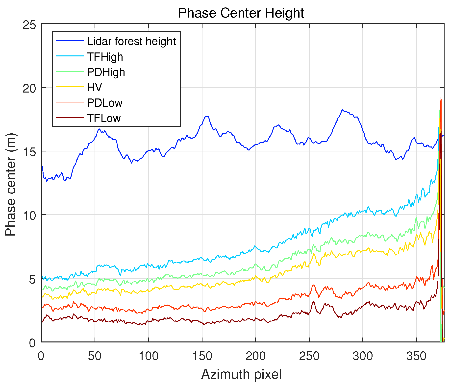
5.1. Phase Center Separation Based on Time-Frequency Optimization

The essence of synthetic aperture is the accumulation of the azimuth time, enabling us to study the radar echo signals related to specific observation angle gaps by selecting the Doppler frequency. Accordingly, the time-frequency analysis enables us to separate the interferometric phase centers from the dimension of the radar observation angle, as different observation angles generally illuminate various scattering mechanisms. For high-frequency SAR systems, the HV channel is commonly deemed to be close to the channel associated with volume scattering, noting that the HV channel does not necessarily correspond directly to a pure volume contribution. Nevertheless, this assumption is no longer valid under P-band observations. As is presented in Figure 11, the HV channel has been quite different from the pure volume channel. Although the coherence optimization acquires a channel, namely γ P D H igh , of which the phase center is higher than that of the HV channel, the time-frequency optimization further effectively separates the phase centers, achieving a higher one (see γ T F H igh in Figure 11). Simultaneously, the phase center of γ T F L ow gained with the time-frequency optimization is also significantly lower than that of γ P D L ow gained with the coherence optimization. Accordingly, the effectiveness of a time-frequency optimization can be directly verified by Figure 11. The result shown in Figure 11 corresponds to the four sublooks situation. As the number of sublook increases, the phase center will be further separated; nonetheless, the loss of the azimuth resolution will become greater [2].

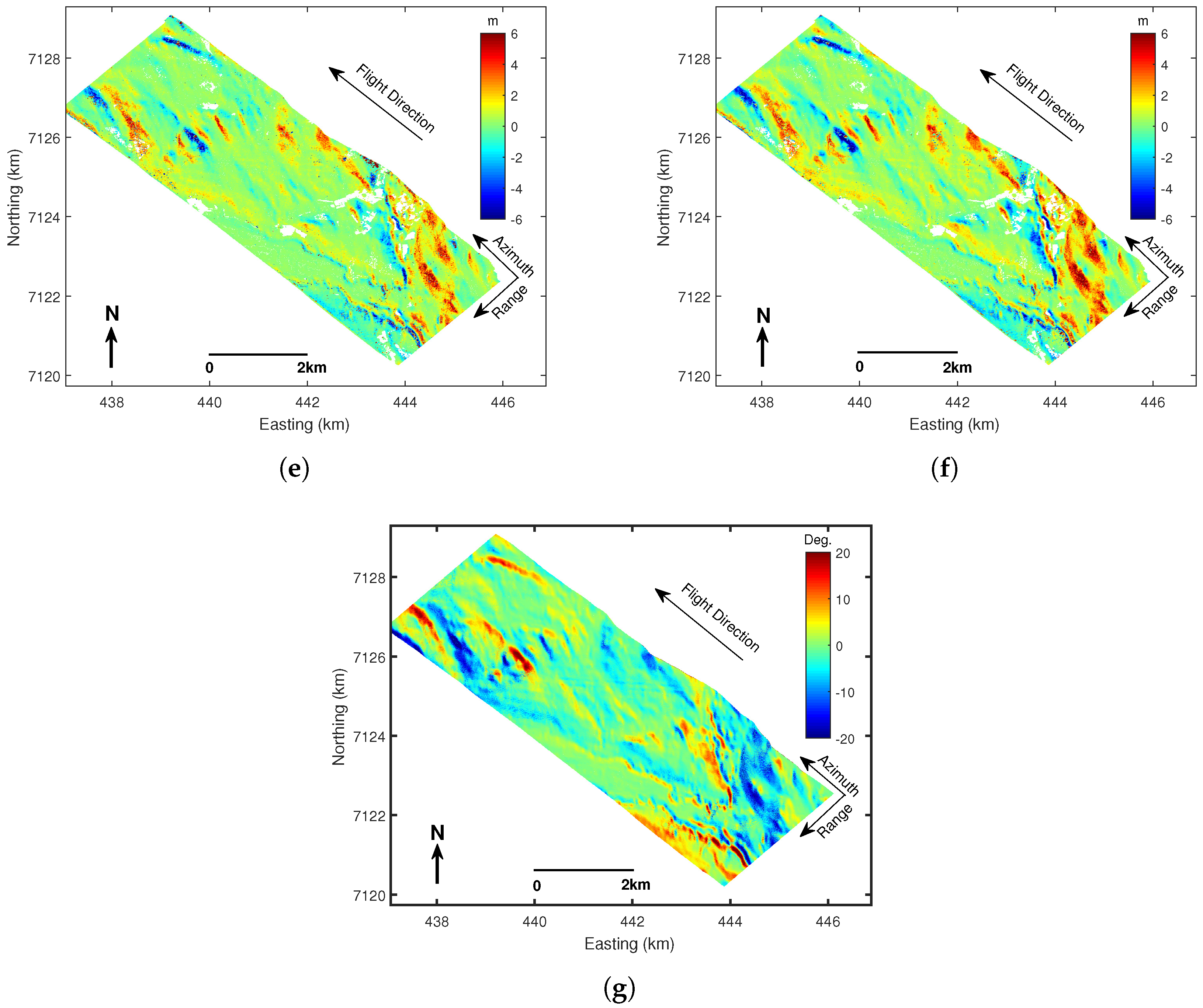
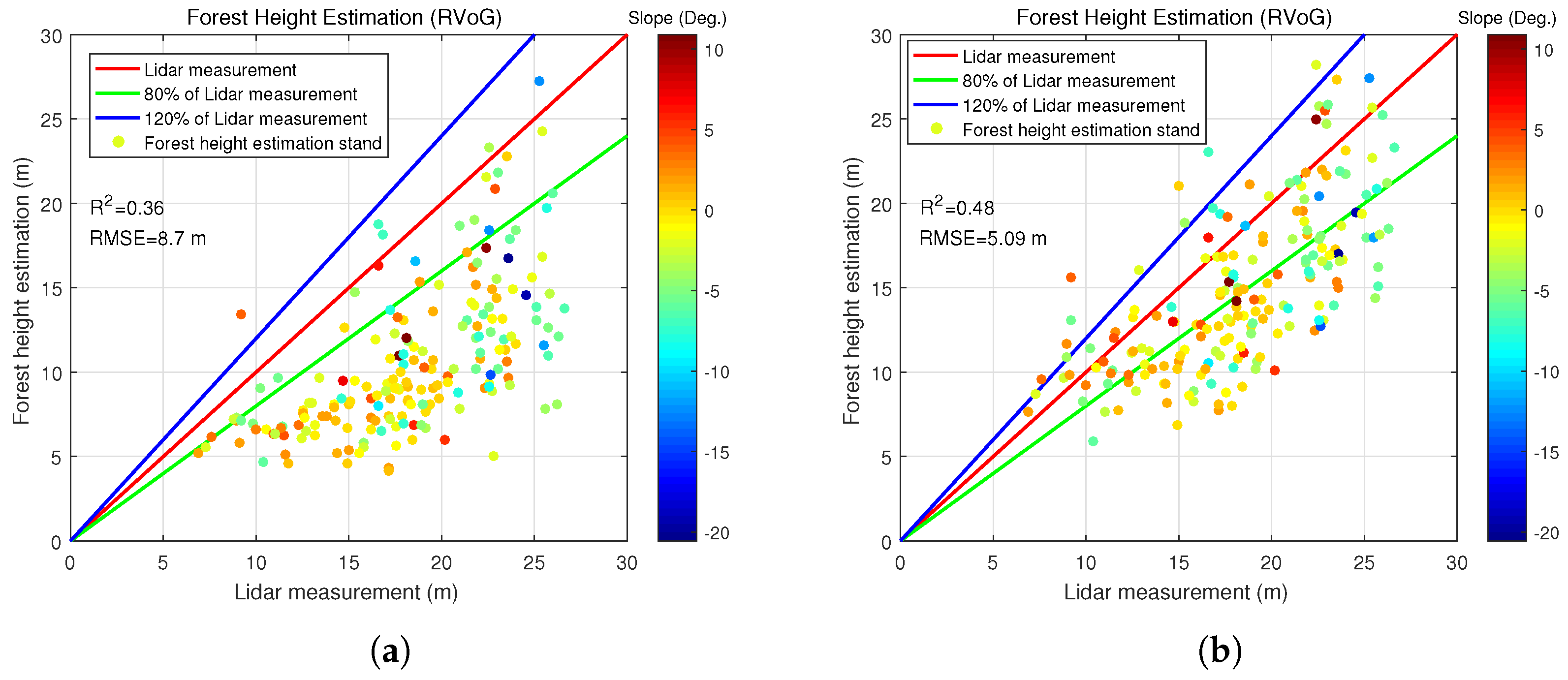
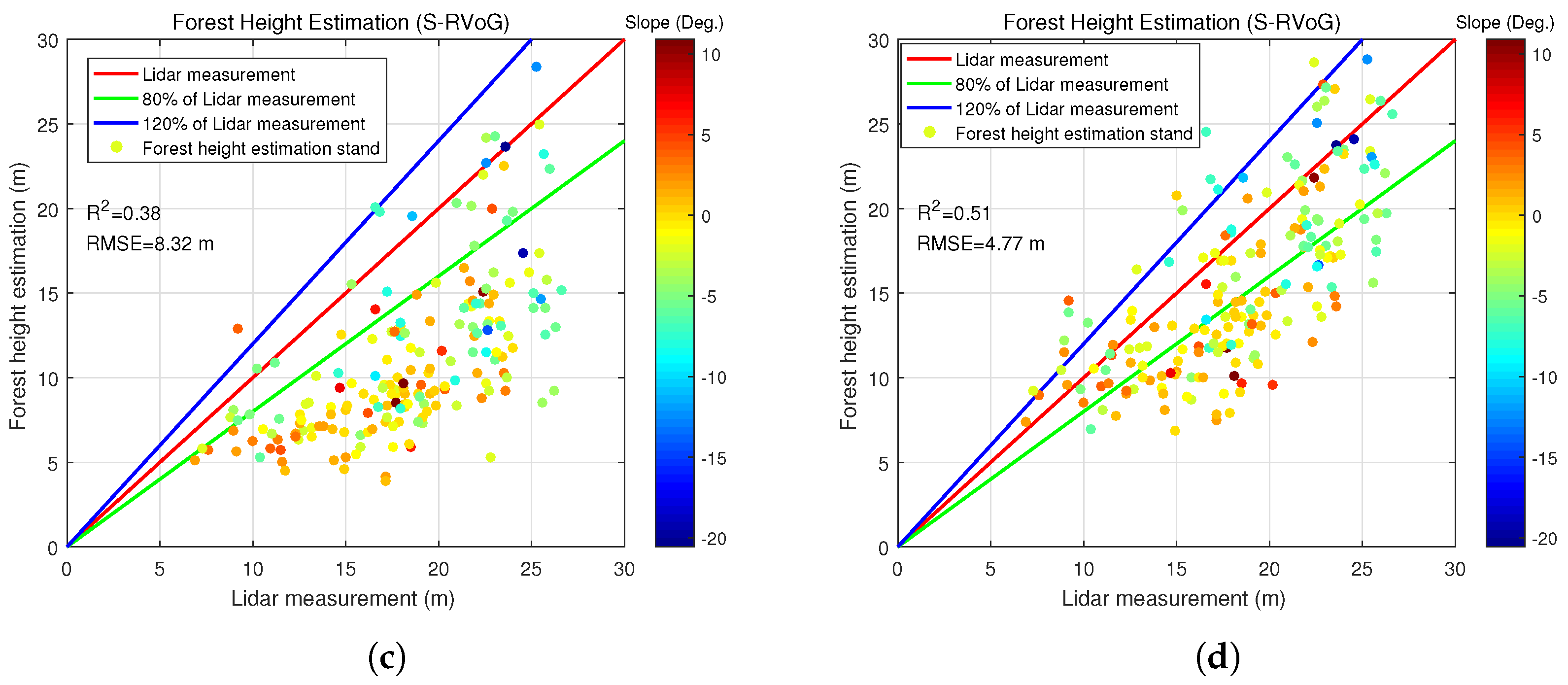
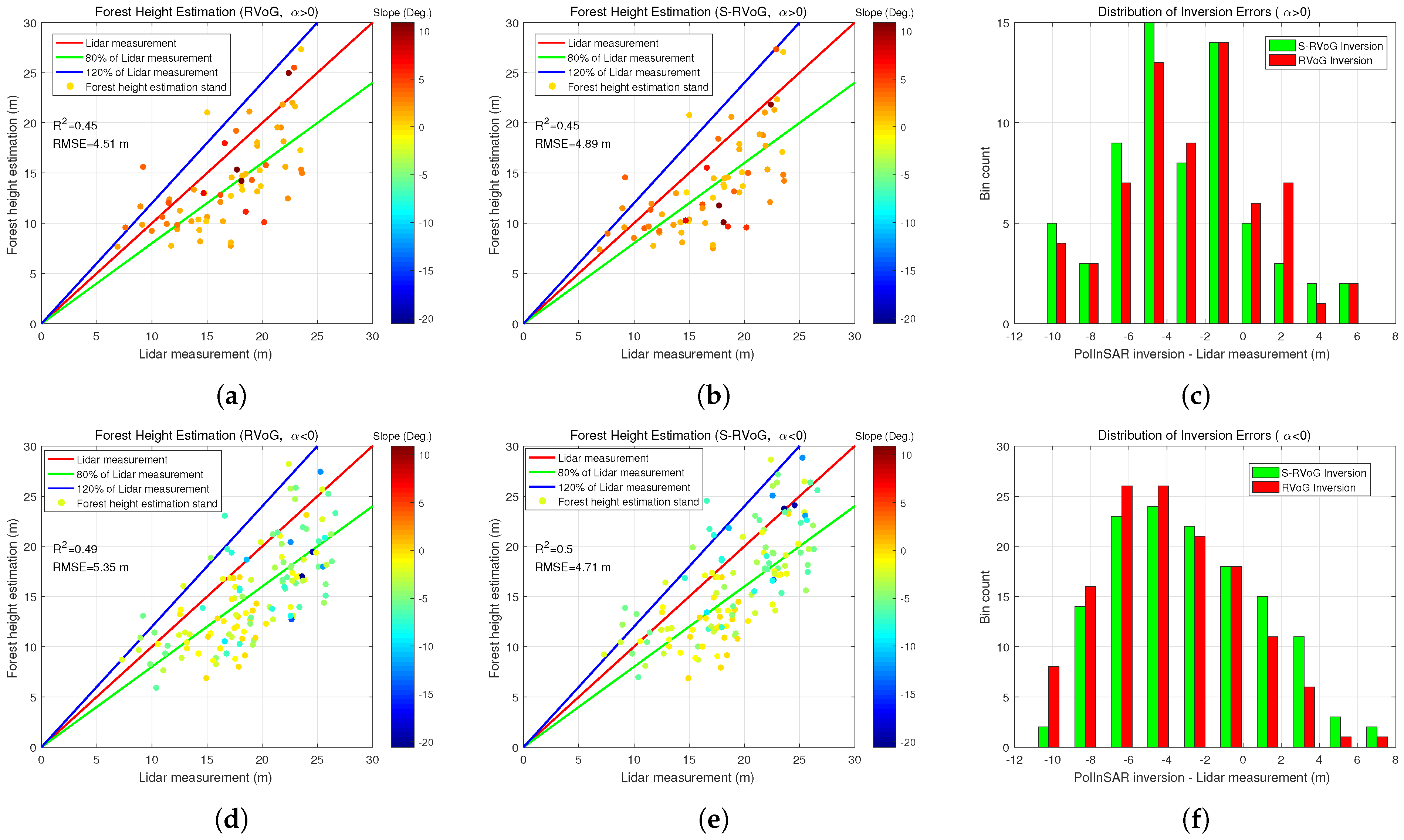
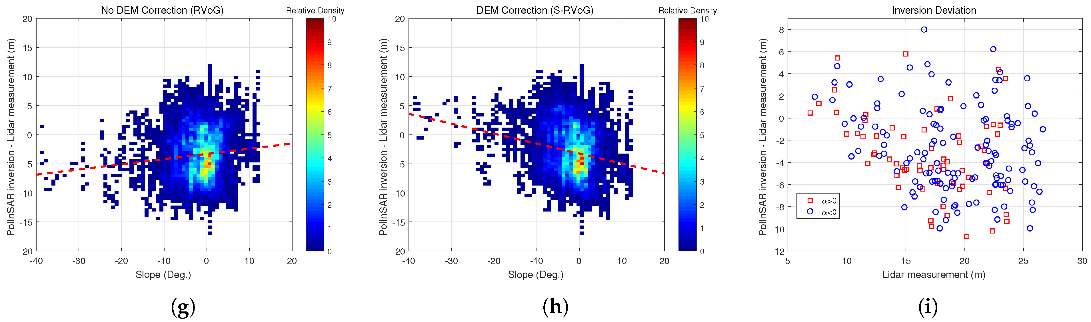
5.2. Effects of Terrain Slope on Inversion Sensitivity

In accordance with Equations (10) and (11), the positive slope increases k z while the negative slope decreases k z . In the light of Equation (12), a larger k z leads to the decrease of coherence and the increase of the phase in the random volume solution space, while a smaller k z leads to an opposite effect. That conclusion is also verified by comparing Figure 2 and Figure 4, from which we can also conclude that the solution space corresponding to a larger k z owns a lower inversion sensitivity, whereas that corresponding to a smaller k z owns a higher inversion sensitivity [6,35]. The homologous experimental results are presented in Figure 12. Consistent with the theoretical analysis, the S-RVoG model on a positive slope reduces the inversion, whereas that on a negative slope rises. Compared with the RVoG model inversion, the S-RVoG model with a negative slope possesses a significantly greater inversion change than that with positive slope, which confirms the conclusion that the negative slope owns a greater inversion sensitivity. In Figure 12a, there are several forest stands of which the inversion changes are located in the scope larger than zero. That accounts for a larger k z comprising a small height of ambiguity. To remove these invalid pixels, we have interpolated these pixels, which brings about the occurrence of anomalous stands in Figure 12a.

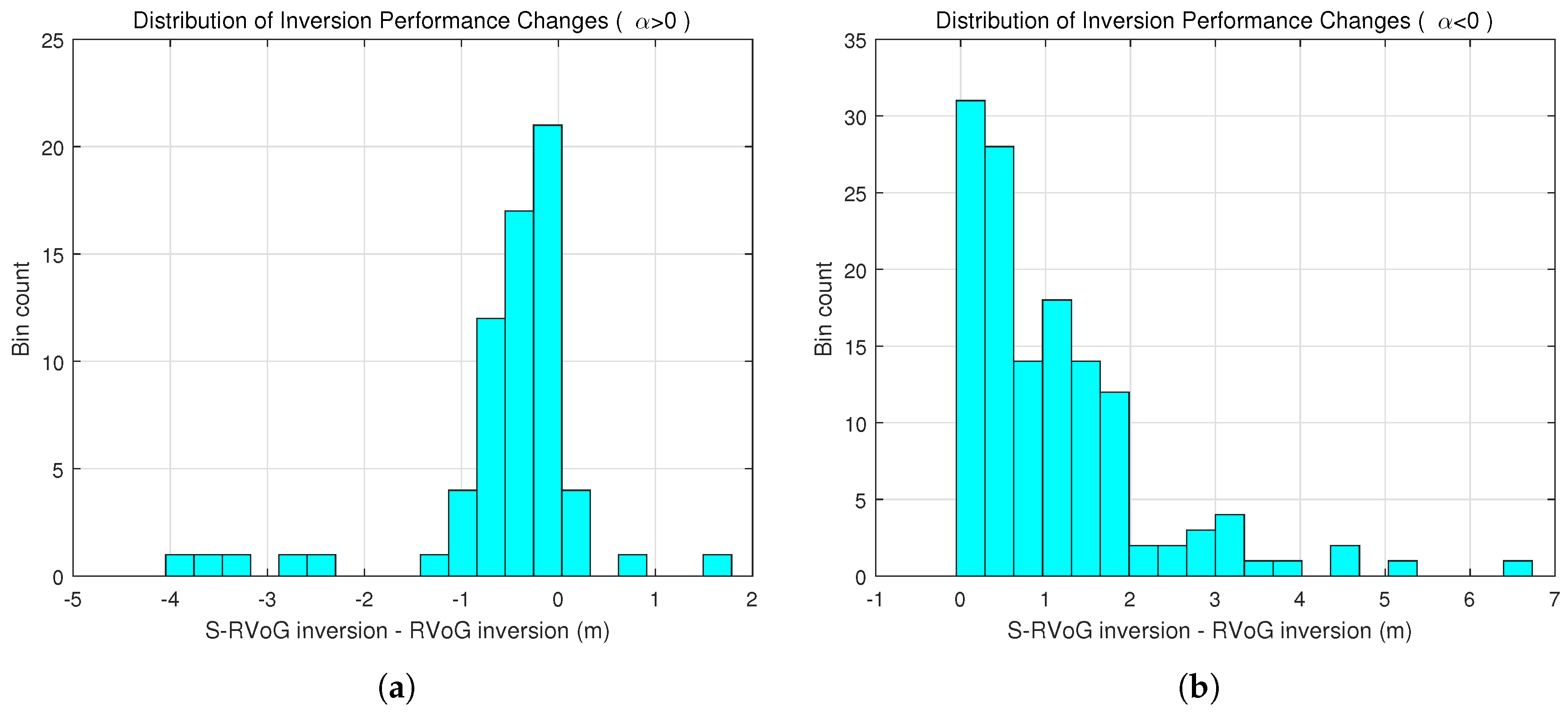
5.3. Discussion on the Quality of Forest Height Estimation

Various forest height estimation methods have been proposed for the P-band data of BIOSAR 2008 campaign [6,32,35,48]. Whether it uses Pol-InSAR or TomoSAR to retrieve forest height, the multi-baseline configuration is a very important solution. In this case, the scheme still using single-baseline configuration requires some prior information. Compared with these studies, the time-frequency optimization is achieved under the single-baseline configuration and does not require specific prior information. Correspondingly, while improving the inversion efficiency, it loses some inversion accuracy. Even so, from the published literature, the performance of this paper is very close to the results of some multi-baseline configurations (such as dual-baseline). To sum up, the proposed method is applicable to the situation that the multi-baseline acquisition cannot be satisfied, there is no specific prior information, a high inversion efficiency is required, and a certain loss of inversion accuracy can be tolerated.

5.4. Limitations of the Proposed Method

From the results discussed in Section 4, even if the time-frequency optimization ameliorates the underestimation of the traditional three-stage method, the underestimation phenomenon still exists. That accounts for at P-band observations all polarimetric channels involving a certain ground contribution. Future research can try to combine the multi-baseline configuration with the time-frequency optimization to avoid the NGVR hypothesis. Another limitation is that the sublook decomposition loses the azimuth resolution of SAR image, and its quantification requires carrying out in future research. The last limitation is that the RVoG model may not be suitable for depicting the vertical backscatter profile of P-band Pol-InSAR as the time-frequency method still cannot completely eliminate the underestimation. That is because the predicted volume coherence is at the boundary (i.e., zero attenuation) of the solution space, which indicates that the situation is beyond the scope of the RVoG model description. The RVoG model deems that the power peak locates at the top of the canopy, nevertheless, when P-band is utilized to observe the boreal forest, backscatter power is chiefly concentrated in the middle and lower parts of the canopy. The way to cope with this limitation is to adopt some new complicated models [35,48,49,50,51].

6. Conclusions

In this paper, we choose the single-baseline configuration for the Pol-InSAR model inversion. Since P-band observations bring about a serious underestimation of the traditional three-stage method, the time-frequency optimization is taken advantage of to mitigate the phenomenon. The phase centers are effectively separated from the dimension of the observation angle, which increases the inversion performance by 41.49%. Furthermore, we take into account the influence of the range terrain slope on inversion, compensating for the three-stage method based on the time-frequency optimization, which improves the inversion performance on negative terrain slope by 11.96%. In summary, this paper provides a scheme on the basis of a time-frequency analysis to solve the Pol-InSAR inversion problem of the single-baseline P-band configuration for sparse vegetation observations. Simultaneously, terrain correction processing is effectively incorporated into this scheme.

Author Contributions

Conceptualization, X.S.; formal analysis, X.S. and X.F.; funding acquisition, B.W., M.X., and Y.L.; investigation, X.S.; methodology, X.S.; project administration, B.W., M.X., and L.Z.; resources, B.W. and M.X.; software, X.S.; supervision, B.W. and M.X.; writing—original draft, X.S.; writing—review and editing, X.S., B.W., M.X., and X.F.

Funding

This research was supported by the Equipment Development Department pre-research fund (No. 61404130308), the National Natural Science Foundation Program of China (No. 41601508) and the Natural Science Foundation Program of Shanghai Municipal (No. 15ZR1439500).

Acknowledgments

The E-SAR data (© ESA 2017) was provided by the European Space Agency (ESA) under the BIOSAR 2008 campaign (ESA EO Project Campaign ID 37708). The ancillary DEM data (© Lantmäteriet) was provided by the Lantmäteriet. The authors would like to thank the anonymous reviewers for their constructive suggestions.

Conflicts of Interest

The authors declare no conflict of interest.

References

  1. Kugler, F.; Koudogbo, F.; Gutjahr, K.; Papathanassiou, K.P. Frequency effects in Pol-InSAR forest height estimation. In Proceedings of the European Conference on Synthetic Aperture Radar, Dresden, Germany, 16–18 May 2006. [Google Scholar]
  2. Garestier, F.; Dubois-Fernandez, P.C.; Champion, I. Forest height inversion using high-resolution P-band Pol-InSAR data. IEEE Trans. Geosci. Remote Sens. 2008, 46, 3544–3559. [Google Scholar] [CrossRef]
  3. Kugler, F.; Lee, S.-K.; Papathanassiou, K.P. Estimation of forest vertical structure parameter by means of multi-baseline Pol-InSAR. In Proceedings of the IEEE International Geoscience and Remote Sensing Symposium, Cape Town, South Africa, 12–17 July 2009; pp. IV-721–IV-724. [Google Scholar]
  4. Garestier, F.; Dubois-Fernandez, P.C.; Guyon, D.; Toan, T.L. Forest biophysical parameter estimation using L- and P-band polarimetric SAR data. IEEE Trans. Geosci. Remote Sens. 2009, 47, 3379–3388. [Google Scholar] [CrossRef]
  5. Lee, S.-K.; Kugler, F.; Hajnsek, I.; Papathanassiou, K.P. The potential and challenges of polarimetric SAR interferometry techniques for forest parameter estimation at P-band. In Proceedings of the European Conference on Synthetic Aperture Radar, Aachen, Germany, 7–10 June 2010; pp. 503–505. [Google Scholar]
  6. Hajnsek, I.; Scheiber, R.; Keller, M.; Horn, R.; Lee, S.-K.; Ulander, L.; Gustavsson, A.; Sandberg, G.; Toan, T.L.; Tebaldini, S. Biosar 2008: Final Report. 2009. Available online: https://earth.esa.int/c/document_library/get_file?folderId=21020&name=DLFE-903.pdf (accessed on 21 November 2018).
  7. Treuhaft, R.N.; Madsen, S.N.; Moghaddam, M.; Van Zyl, J.J. Vegetation characteristics and underlying topography from interferometric radar. Radio Sci. 1996, 31, 1449–1485. [Google Scholar] [CrossRef]
  8. Cloude, S.R.; Papathanassiou, K.P. Polarimetric SAR interferometry. IEEE Trans. Geosci. Remote Sens. 1998, 36, 1551–1565. [Google Scholar] [CrossRef]
  9. Treuhaft, R.N.; Siqueira, P.R. Vertical structure of vegetated land surfaces from interferometric and polarimetric radar. Radio Sci. 2000, 35, 141–177. [Google Scholar] [CrossRef]
  10. Papathanassiou, K.P.; Cloude, S.R. Single-baseline polarimetric SAR interferometry. IEEE Trans. Geosci. Remote Sens. 2001, 39, 2352–2363. [Google Scholar] [CrossRef]
  11. Cloude, S.R. Robust parameter estimation using dual baseline polarimetric SAR interferometry. In Proceedings of the IEEE International Geoscience and Remote Sensing Symposium, Toronto, ON, Canada, 24–28 June 2002; pp. 838–840. [Google Scholar]
  12. Cloude, S.R.; Papathanassiou, K.P. Three-stage inversion process for polarimetric SAR interferometry. IEE Proc. Radar Sonar Navig. 2003, 150, 125–134. [Google Scholar] [CrossRef]
  13. Mette, T.; Kugler, F.; Papathanassiou, K.P.; Hajnsek, I. Forest and the random volume over ground-nature and effect of 3 possible error types. In Proceedings of the European Conference on Synthetic Aperture Radar, Dresden, Germany, 16–18 May 2006. [Google Scholar]
  14. Garestier, F.; Dubois-Fernandez, P.C.; Papathanassiou, K.P. Pine forest height inversion using single-pass X-band PolInSAR data. IEEE Trans. Geosci. Remote Sens. 2008, 46, 59–68. [Google Scholar] [CrossRef]
  15. Cloude, S.R. Polarisation: Applications in Remote Sensing; Oxford University Press: New York, NY, USA, 2009. [Google Scholar]
  16. Roueff, A.; Arnaubec, A.; Dubois-Fernandez, P.C.; Refregier, P. Cramer-rao lower bound analysis of vegetation height estimation with random volume over ground model and polarimetric SAR interferometry. IEEE Geosci. Remote Sens. Lett. 2011, 8, 1115–1119. [Google Scholar] [CrossRef]
  17. Neumann, M.; Saatchi, S.S.; Ulander, L.M.; Fransson, J.E. Assessing performance of L-and P-band polarimetric interferometric SAR data in estimating boreal forest above-ground biomass. IEEE Trans. Geosci. Remote Sens. 2012, 50, 714–726. [Google Scholar] [CrossRef]
  18. Lopez-Martinez, C.; Alonso-Gonzalez, A. Assessment and estimation of the RVoG model in polarimetric SAR interferometry. IEEE Trans. Geosci. Remote Sens. 2014, 52, 3091–3106. [Google Scholar] [CrossRef]
  19. Lei, Y.; Siqueira, P. Estimation of forest height using spaceborne repeat-pass L-band InSAR correlation magnitude over the US state of Maine. Remote Sens. 2014, 6, 10252–10285. [Google Scholar] [CrossRef]
  20. Ballester-Berman, J.D.; Vicente-Guijalba, F.; Lopez-Sanchez, J.M. A simple RVoG test for PolInSAR data. IEEE J. Sel. Top. Appl. Earth Obs. Remote Sens. 2015, 8, 1028–1040. [Google Scholar] [CrossRef]
  21. Papathanassiou, K.P.; Cloude, S.R. The effect of temporal decorrelation on the inversion of forest parameters from PoI-InSAR data. In Proceedings of the IEEE International Geoscience and Remote Sensing Symposium, Toulouse, France, 21–25 July 2003. [Google Scholar]
  22. Lee, S.-K.; Kugler, F.; Papathanassiou, K.P.; Hajnsek, I. Quantifying temporal decorrelation over boreal forest at L-and P-band. In Proceedings of the European Conference on Synthetic Aperture Radar, Friedrichshafen, Germany, 2–5 June 2008. [Google Scholar]
  23. Ahmed, R.; Siqueira, P.; Hensley, S.; Chapman, B.; Bergen, K. A survey of temporal decorrelation from spaceborne L-band repeat-pass InSAR. Remote Sens. Environ. 2011, 115, 2887–2896. [Google Scholar] [CrossRef]
  24. Simard, M.; Hensley, S.; Lavalle, M.; Dubayah, R.; Pinto, N.; Hofton, M. An empirical assessment of temporal decorrelation using the uninhabited aerial vehicle synthetic aperture radar over forested landscapes. Remote Sens. 2012, 4, 975–986. [Google Scholar] [CrossRef]
  25. Lavalle, M.; Simard, M.; Hensley, S. A temporal decorrelation model for polarimetric radar interferometers. IEEE Trans. Geosci. Remote Sens. 2012, 50, 2880–2888. [Google Scholar] [CrossRef]
  26. Neumann, M.; Ferro-Famil, L.; Reigber, A. Estimation of forest structure, ground, and canopy layer characteristics from multibaseline polarimetric interferometric SAR data. IEEE Trans. Geosci. Remote Sens. 2010, 48, 1086–1104. [Google Scholar] [CrossRef]
  27. Hajnsek, I.; Kugler, F.; Lee, S.-K.; Papathanassiou, K.P. Tropical-forest-parameter estimation by means of Pol-InSAR: The INDREX-II campaign. IEEE Trans. Geosci. Remote Sens. 2009, 47, 481–493. [Google Scholar] [CrossRef]
  28. Park, S.E.; Moon, W.M.; Pottier, E. Assessment of scattering mechanism of polarimetric SAR signal from mountainous forest areas. IEEE Trans. Geosci. Remote Sens. 2012, 50, 4711–4719. [Google Scholar] [CrossRef]
  29. Lu, H.; Suo, Z.; Guo, R.; Bao, Z. S-RVoG model for forest parameters inversion over underlying topography. Electron. Lett. 2013, 49, 618–620. [Google Scholar] [CrossRef]
  30. Kugler, F.; Lee, S.-K.; Hajnsek, I.; Papathanassiou, K.P. Forest height estimation by means of Pol-InSAR data inversion: The role of the vertical wavenumber. IEEE Trans. Geosci. Remote Sens. 2015, 53, 5294–5311. [Google Scholar] [CrossRef]
  31. Zhang, Q.; Liu, T.; Ding, Z.; Zeng, T.; Long, T. A modified three-stage inversion algorithm based on R-RVoG model for Pol-InSAR data. Remote Sens. 2016, 8, 861. [Google Scholar] [CrossRef]
  32. Xie, Q.; Zhu, J.; Wang, C.; Fu, H.; Lopezsanchez, J.M.; Ballesterberman, J.D. A modified dual-baseline PolInSAR method for forest height estimation. Remote Sens. 2017, 9, 819. [Google Scholar] [CrossRef]
  33. Fu, W.; Guo, H.; Li, X.; Tian, B.; Sun, Z. Extended three-stage polarimetric SAR interferometry algorithm by dual-polarization data. IEEE Trans. Geosci. Remote Sens. 2016, 54, 2792–2802. [Google Scholar]
  34. Managhebi, T.; Maghsoudi, Y.; Zoej, M.J.V. An improved three-stage inversion algorithm in forest height estimation using single-baseline polarimetric sar interferometry data. IEEE Geosci. Remote Sens. Lett. 2018, 15, 887–891. [Google Scholar] [CrossRef]
  35. Sun, X.; Wang, B.; Xiang, M.; Jiang, S.; Fu, X. Forest height estimation based on constrained Gaussian vertical backscatter model using multi-baseline P-band Pol-InSAR data. Remote Sens. 2019, 11, 42. [Google Scholar] [CrossRef]
  36. Lavalle, M.; Khun, K. Three-baseline InSAR estimation of forest height. IEEE Geosci. Remote Sens. Lett. 2014, 11, 1737–1741. [Google Scholar] [CrossRef]
  37. Lee, S.-K.; Kugler, F.; Papathanassiou, K.P.; Hajnsek, I. Multibaseline polarimetric SAR interferometry forest height inversion approaches. In Proceedings of the ESA PolInSAR Workshop, Frascati, Italy, 24–28 January 2011. [Google Scholar]
  38. Ferro-Famil, L.; Neumann, M.; Huang, Y. Multi-baseline Pol-InSAR statistical techniques for the characterization of distributed media. In Proceedings of the IEEE International Geoscience and Remote Sensing Symposium, Cape Town, South Africa, 12–17 July 2009; pp. III-971–III-974. [Google Scholar]
  39. Treuhaft, R.N.; Cloude, S.R. The structure of oriented vegetation from polarimetric interferometry. IEEE Trans. Geosci. Remote Sens. 1999, 37, 2620–2624. [Google Scholar] [CrossRef]
  40. Lopez-Sanchez, J.M.; Ballester-Berman, J.D.; Marquez-Moreno, Y. Model limitations and parameter-estimation methods for agricultural applications of polarimetric SAR interferometry. IEEE Trans. Geosci. Remote Sens. 2007, 45, 3481–3493. [Google Scholar] [CrossRef]
  41. Pichierri, M.; Hajnsek, I.; Papathanassiou, K.P. A multibaseline Pol-InSAR inversion scheme for crop parameter estimation at different frequencies. IEEE Trans. Geosci. Remote Sens. 2016, 54, 4952–4970. [Google Scholar] [CrossRef]
  42. Cumming, I.G.; Wong, F.H. Digital Processing of Synthetic Aperture Radar Data: Algorithms and Implementation; ArtechHouse: Boston, MA, USA, 2005. [Google Scholar]
  43. Dubois, P.C.; Rignot, E.; Van Zyl, J.J. Direction angle sensitivity of agricultural field backscatter with Airsar data. In Proceedings of the IEEE International Geoscience and Remote Sensing Symposium, Houston, TX, USA, 26–29 May 1992; pp. 1680–1681. [Google Scholar]
  44. Souyris, J.C.; Henry, C.; Adragna, F. On the use of complex SAR image spectral analysis for target detection: Assessment of polarimetry. IEEE Trans. Geosci. Remote Sens. 2003, 41, 2725–2734. [Google Scholar] [CrossRef]
  45. Ferro-Famil, L.; Reigber, A.; Pottier, E.; Boerner, W.M. Scene characterization using subaperture polarimetric SAR data. IEEE Trans. Geosci. Remote Sens. 2003, 41, 2264–2276. [Google Scholar] [CrossRef]
  46. Fu, H.; Zhu, J.; Wang, C.; Wang, H.; Zhao, R. Underlying topography estimation over forest areas using high-resolution P-band single-baseline PolInSAR data. Remote Sens. 2017, 9, 363. [Google Scholar] [CrossRef]
  47. Tabb, M.; Orrey, J.; Flymn, T.; Carande, R. Phase diversity: A decomposition for vegetation parameter estimation using polarimetric SAR interferometry. In Proceedings of the European Conference on Synthetic Aperture Radar, Cologne, Germany, 4–6 June 2002; pp. 721–724. [Google Scholar]
  48. Fu, H.; Wang, C.; Zhu, J.; Xie, Q.; Zhang, B. Estimation of pine forest height and underlying dem using multi-baseline P-band PolInSAR data. Remote Sens. 2016, 8, 820. [Google Scholar] [CrossRef]
  49. Garestier, F.; Toan, T.L. Forest modeling for height inversion using single-baseline InSAR/Pol-InSAR data. IEEE Trans. Geosci. Remote Sens. 2010, 48, 1528–1539. [Google Scholar] [CrossRef]
  50. Garestier, F.; Toan, T.L. Estimation of the backscatter vertical profile of a pine forest using single baseline P-band (Pol-)InSAR data. IEEE Trans. Geosci. Remote Sens. 2010, 48, 3340–3348. [Google Scholar] [CrossRef]
  51. Sun, X.; Zhou, L.; Wang, B.; Li, W.; Xiang, M.; Jiang, S. A new model for P-band Pol-InSAR based on Gamma distribution. In Proceedings of the IEEE International Geoscience and Remote Sensing Symposium, Valencia, Spain, 22–27 July 2018; pp. 5867–5870. [Google Scholar]
Figure 1. The schematic representation of the synthetic aperture (top), Doppler history (center), and Doppler spectra (bottom) during the synthetic aperture time.
Remotesensing 11 01033 g001
Figure 2. The schematic representation of the RVoG model. The theoretical random volume coherences are exhibited in blue curves for the forest height and mean extinction coefficient ranging, respectively, from 5 to 30 m and 0.02 to 2 dB/m in accordance with Equation (5). Each curve matches a given forest height between which the interval is 1 m. The measured forest height is 19 m, and the homologous volume coherences are indicated by the pink curve. The incidence angle and interferometric vertical wavenumber are set to 0.8 rad and 0.15 rad/m, respectively. The unit circle has been rotated by the ground interferometric phase compensation.
Remotesensing 11 01033 g002
Figure 3. The interferometric acquisition geometry with range terrain slope: (a) The positive terrain slope and (b) the negative terrain slope. α is the range terrain slope, S m and S s are the master and slave antennas respectively, B H is the horizontal baseline, θ is the incidence angle, Δ θ is the difference of incidence angle between master and slave antennas, θ is the local incidence angle, y o z and y o z are the original and corrected coordinate system respectively, h v is the forest height estimation in the corrected coordinate system, and h v is the final estimation.
Remotesensing 11 01033 g003
Figure 4. The schematic representation of the S-RVoG model: (a) The positive terrain slope (5 deg) and (b) the negative terrain slope (−5 deg). The parameter setting of the theoretical sloped random volume coherence is consistent with Figure 2. The green and pink curves represent the volume coherences corresponding to a 19-m forest height based on the RVoG and S-RVoG models, respectively. The green dots denote the coherence estimation.
Remotesensing 11 01033 g004
Figure 5. The schematic representation of the S-RVoG model inversion: The parameter setting of the theoretical sloped random volume cohernce is consistent with Figure 4a (corresponding to a 5 deg terrain slope). The pink curve represents the volume coherences corresponding to a 19-m forest height based on the S-RVoG model while the green curve represents the volume coherences for a 0 dB/m extinction. The green dots denote the coherence estimation. The blue dot indicates the predicted volume coherence. The black dotted line represents the minimum route between γ T F H igh and the solution space.
Remotesensing 11 01033 g005
Figure 6. The flowchart of the S-RVoG model inversion based on the time-frequency optimization.
Remotesensing 11 01033 g006
Figure 7. (a) The Pauli-basis polarimetric composite map, (b) measured DEM, and (c) Lidar-derived forest height.
Remotesensing 11 01033 g007
Figure 8. The forest height estimation with (a) RVoG model + three-stage method, (b) RVoG model + modified three-stage method (time-frequency optimization), (c) S-RVoG model + three-stage method, and (d) S-RVoG model + modified three-stage method (time-frequency optimization). (e,f) The difference values after terrain compensation corresponding to Figure 8a,c and Figure 8b,d, respectively. (g) The range terrain slope.
Remotesensing 11 01033 g008aRemotesensing 11 01033 g008b
Figure 9. The forest height estimation of validation stands with (a) RVoG model + three-stage method, (b) RVoG model + modified three-stage method (time-frequency optimization), (c) S-RVoG model + three-stage method, and (d) S-RVoG model + modified three-stage method (time-frequency optimization), compared with the lidar measurement. The color of the dots represents the terrain slope.
Remotesensing 11 01033 g009aRemotesensing 11 01033 g009b
Figure 10. The forest height estimation of validation stands (corresponding to slope α > 0 deg) with the RVoG model (a) and the S-RVoG model (b), compared with the lidar measurement. The forest height estimation of validation stands (corresponding to slope α < 0 deg) with the RVoG model (d) and the S-RVoG model (e), compared with the lidar measurement, respectively. The color of the dots represents the terrain slope. (c) The histogram of the difference between the PolInSAR inversion and lidar measurement with the RVoG model and the S-RVoG model, respectively. The stands that are counted correspond to the stands in (a,b). (f) The histogram of the difference between the PolInSAR inversion and lidar measurement with the RVoG model and the S-RVoG model, respectively. The stands that are counted correspond to the stands in Figure 10d,e. (g) The slope versus height difference between the PolInSAR inversion without terrain correction and the lidar measurement. (h) The slope versus height difference between the PolInSAR inversion with terrain correction and the lidar measurement. The red dashed lines in Figure 10g,h are acquired by a linear fitting of all the density points. (i) The deviation between the S-RVoG model inversion and the lidar measurement.
Remotesensing 11 01033 g010aRemotesensing 11 01033 g010b
Figure 11. The phase center height for different polarimetric channels. The phase center height has been processed by averaging along the azimuth direction.
Remotesensing 11 01033 g011
Figure 12. The distribution of inversion performance changes for α > 0 (a) and α < 0 (b).
Remotesensing 11 01033 g012
Table 1. The parameters of the interferometric pair.
TrackBaseline (m) k z RangeBandPolarization
MasterMasterMasterPQuad
Slave320.026–0.245PQuad

