Local Deep Descriptor for Remote Sensing Image Feature Matching
by
 , ,
, ,
Yunyun Dong
1,2 ,
,
Weili Jiao
1,*,
Tengfei Long
1,*,
Lanfa Liu
3,
Guojin He
1,
Chengjuan Gong
1,2 and
Yantao Guo
1,2 1
Aerospace Information Research Institute, Chinese Academy of Sciences, Beijing 100094, China
2
University of Chinese Academy of Sciences, Beijing 100049, China
3
Institute for Cartography, TU Dresden, 01062 Dresden, Germany
*
Authors to whom correspondence should be addressed.
Remote Sens. 2019, 11(4), 430; https://0-doi-org.brum.beds.ac.uk/10.3390/rs11040430
Submission received: 3 January 2019
/
Revised: 2 February 2019
/
Accepted: 15 February 2019
/
Published: 19 February 2019
(This article belongs to the Special Issue Image Processing and Analysis: Trends in Registration, Data Fusion, 3D Reconstruction and Change Detection)
Abstract
:Feature matching via local descriptors is one of the most fundamental problems in many computer vision tasks, as well as in the remote sensing image processing community. For example, in terms of remote sensing image registration based on the feature, feature matching is a vital process to determine the quality of transform model. While in the process of feature matching, the quality of feature descriptor determines the matching result directly. At present, the most commonly used descriptor is hand-crafted by the designer’s expertise or intuition. However, it is hard to cover all the different cases, especially for remote sensing images with nonlinear grayscale deformation. Recently, deep learning shows explosive growth and improves the performance of tasks in various fields, especially in the computer vision community. Here, we created remote sensing image training patch samples, named Invar-Dataset in a novel and automatic way, then trained a deep learning convolutional neural network, named DescNet to generate a robust feature descriptor for feature matching. A special experiment was carried out to illustrate that our created training dataset was more helpful to train a network to generate a good feature descriptor. A qualitative experiment was then performed to show that feature descriptor vector learned by the DescNet could be used to register remote sensing images with large gray scale difference successfully. A quantitative experiment was then carried out to illustrate that the feature vector generated by the DescNet could acquire more matched points than those generated by hand-crafted feature Scale Invariant Feature Transform (SIFT) descriptor and other networks. On average, the matched points acquired by DescNet was almost twice those acquired by other methods. Finally, we analyzed the advantages of our created training dataset Invar-Dataset and DescNet and gave the possible development of training deep descriptor network.
1. Introduction
Feature matching is the basis of various remote sensing processing tasks, such as image retrieval [1,2], object recognition [3,4] and image registration [5,6,7,8]. eature matching can also contribute to calibrate attitude sensor performance [9,10]. Taking remote sensing registration as an example, feature based methods are also mainstream methods in the practical application. Although image registration methods based on area do not need to extract and match features, they are sensitive to gray changes [11,12], or are only able to deal with simple geometric deformation, such as translation [13] or similarity transform [14,15]. However, for feature based remote sensing image registration, the acquired number of matched points is vital for estimating the final transform model. If the number of matched points is not enough large, the estimated transform model will be biased or even false [16,17,18,19]. For feature matching, there are two main variables: Feature descriptor and similarity measurement. The feature descriptor is always the core and the similarity measurement is dependent on feature descriptors. However, manually designed SIFT (Scale Invariant Feature Transform) [20] descriptors may be unable to take into in an optimal manner all the changes in image appearance, such as different viewpoints, different resolution, nonlinear brightness distortions, geometric deformations, geometric characteristic of objects, occlusions and so on. In the community of the remote sensing images, due to the specialty of remote sensing images, the SIFT and its variants designed for natural images do not always perform well [16]. Especially for non-linear brightness variation, one common problem in remote sensing images is that the calculated principal direction of the SIFT feature point are unreliable, because of the varieties of the statistic of gradients around the feature point. This problem will produce many false matched points or fewer matched points, which results in a mis-registration or failure of registration. So, the descriptor of feature points detected from images with non-linear brightness variation is a bottleneck problem for remote sensing image further processing, especially for the registration task.
Motivated by the recent success in computer vision tasks with deep convolutional neural networks, such as scene classification [21], object recognition [22], image segmentation [23], image retrieval [24] and so on, we utilized deep learning technology to tackle the problem by encoding image patches. For natural images, deep convolutional neural networks [25,26] has gained the superiority in the comparison of image patches over the traditional descriptors, such as SIFT descriptors [20] and DAISY descriptors [27]. However, due to the lack of large amount of remote sensing image corresponding patches and challenges of remote sensing image patch correspondence, such as the variation of image content acquired at different time and brightness distortion of multi-source images, the existing models do not apply to the comparison of remote sensing image patches directly.
Here, we created a remote sensing image training patches in a novel and automatic way and then trained a novel deep convolutional network from scratch to generate a robust feature point descriptor. At last we utilized the learned descriptor to replace the hand-crafted descriptor and fulfil the feature matching. We carried out extensive experiments to illustrate the superiority of our created training samples and the proposed network qualitatively and quantitatively.
In summary, our main contributions were as follows:
- (1)
- In the case of creation of training dataset, we created a large amount of remote sensing image patches in a novel and automatic way (namely that there is no need to extract and label image patch sample manually, as will be detailed in the Section 3.2), which are different from an extraction from the original image directly. They make it possible to apply deep learning in the remote sensing feature matching in a low-cost way. And they enable the deep convolutional neural network to generate a better description vector for each feature point.
- (2)
- In the case of building architecture of deep convolutional neural network, we utilized a new deep convolutional neural network to describe the feature points detected from the remote sensing images. Compared to other popular networks and traditional hand-crafted SIFT descriptors, it can achieve much more corresponding feature points effectively and have a much higher average inlier ratio.
- (3)
- In the case of training processing, because the number of non-corresponding patches generated online is much larger than the one of corresponding patches and iteration over all the negative samples is impossible, we applied the strategy of aggressive mining of ‘hardest’ samples instead of selecting some of negatives randomly, which promoted the convolutional network to learn fully from samples in each epoch. This not only accelerated the training process and but also improved the performance of the network.
The rest of the paper is organized as follows. Section 2 introduces the related work of natural image patch comparison based on the deep convolutional network. Section 3 details our proposed methodology. Section 4 presents the qualitative and quantitative experiments. The discussion is given in Section 5. The conclusions are drawn in Section 6.
2. Related Work
Since the deep convolutional neural network Alex-Net has achieved top-1 recognition performance by a large margin than traditional algorithms in the ImageNet LSVRC-2012 contest in 2012 [28], deep learning has entered a new period of explosive growth, especially in the community of computer vision. New data-driven, learned algorithms are replacing the traditional rule-based algorithms through their excellent performance. In recent years, the performance of comparing image patches has also improved greatly by the introduction of the deep convolutional neural network and larger image datasets. In general, researchers are focusing on four aspects to improve the performance of comparing patches based on deep convolutional neural network, namely the architecture of the convolutional neural network, training strategy, training data and loss function.
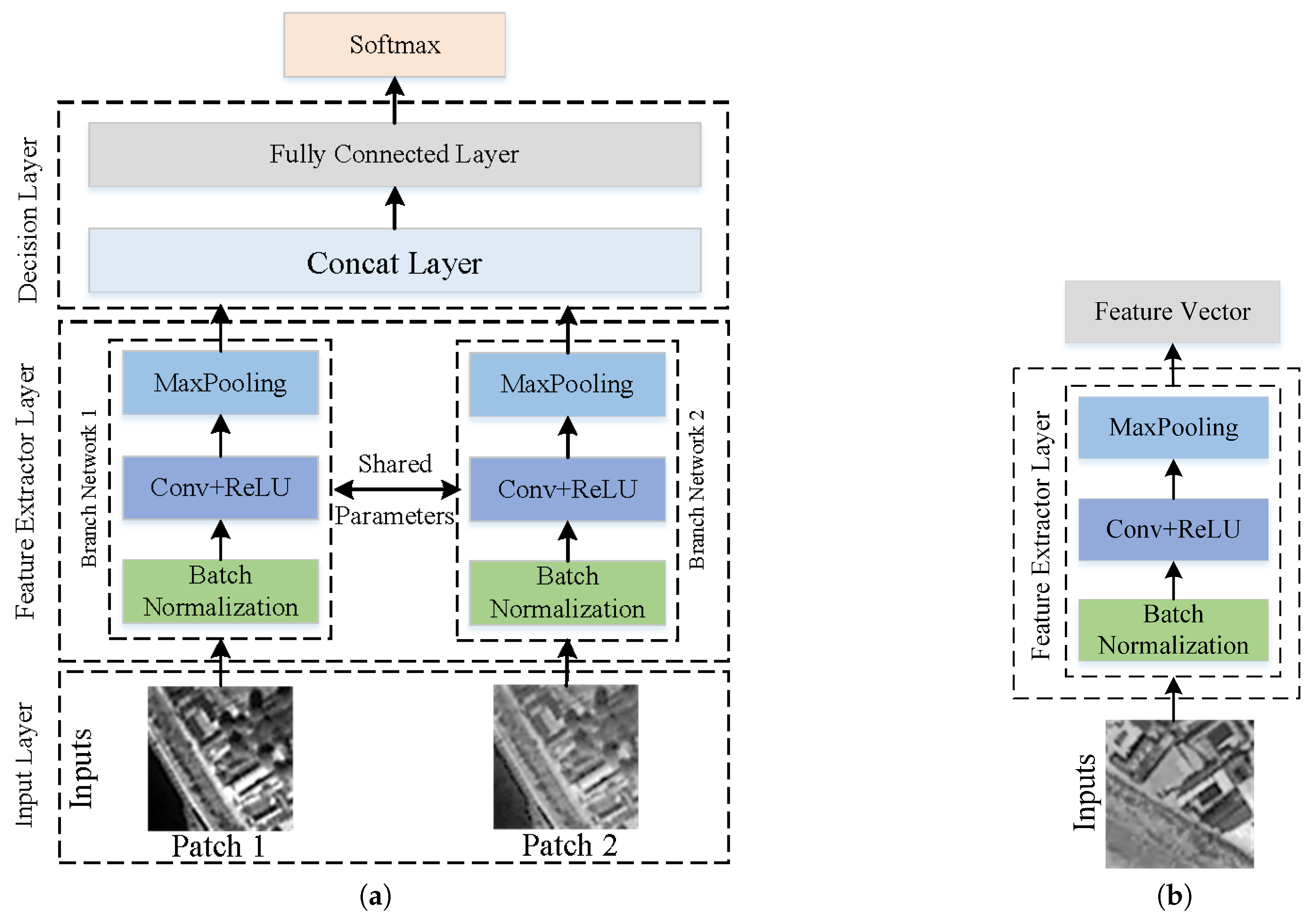
For the architecture of convolutional neural network, the basic architecture can be divided into two categories, one being the Siamese network and the other being the non-Siamese network. Their network structures are shown in Figure 1. The Siamese network, also known as the two-branch structure with tied parameters, makes a basic assumption that each patch goes through the same feature encoding network before measuring the similarity of feature descriptors. Therefore, there is only one feature network in fact. It consists of an input layer, a batch normalization layer, a pooling layer, a concat layer, a fully connected layer and a softmax layer. The batch normalization layer [29] adjusts and scales the value of the layer to accelerate the training of network and be less sensitive to the parameters initialization. Concat layer is utilized to concatenate the two 1-D vectors in the 0-th dimension to obtain a more long vector. Softmax is a non-linear function, it maps each element of the vector to the range (0,1) and sum to 1. The core function of the feature network is mapping each patch into the same feature space then differentiating their difference. It’s advantage is that it can acquire a higher performance of determining corresponding image patches due to the tight combination of the feature extraction layers and metric learning layers. At the same time, its disadvantage is also evident: Poor versatility. For example, it is difficult to be applied in the case of feature point matching based on nearest neighbor distance due to the high time complexity. Because the inputs of the Siamese network must be a pair of patches, for points set with size of and points set with size of , take a point from as example, pairs of patches will be formed to determine the final corresponding point. The total time complexity is , and there is only the brute force algorithm to complete the task. In fact, this inefficiency is unacceptable in practical application. For the non-Siamese network, however, the input is a single patch and the output is a feature vector, two feature vector sets can be acquired, and a quick nearest search algorithm of kd-tree can be utilized to finish the task efficiently. The most representative network is MatchNet [25]. Compared to the Siamese network, the non-Siamese network has only one single model, which plays a role of feature encoder. Each patch going through the model is converted to a fixed-dimension vector. The representative networks are Hardnet [30], L2-Net [26] and TFeat [31]. It has great versatility and can be used to deal with many tasks, such as image retrieval, verification and matching. In this paper, we aimed to get grid of the metric learning layers and only explore a feature network with high performance to generate a good descriptor of a feature point. It could replace the traditional hand-designed descriptors and be utilized to find more correct corresponding points to improve the registration accuracy of remote sensing further.
Due to the large number of parameters of network, huge parameter space and the nonconvexity of loss function, finding an optimal solution is a very difficult task. So, in the training process, some effective strategies and tricks are vital to achieve a network with good performance within limited computing resources and time frames. Recently, a bag of training tricks to improve the performance of network were surveyed in [32], such as the selection and setting of an optimization method, including the initial learning rate value, learning rate decay schedule and other hyper parameter settings, data augmentation methods, including flip horizontally, random crop, color jitter, the addition of random noise and so on. Experimental results showed that a proper trick could bring an additional performance improvement to the network. Due to the lack of a solid interpretation of these tricks, although some tricks may can improve the performance, it was hard to select a proper trick to train deep convolution network without prior testing. So, in our specific training process, we tried different tricks and different combinations to improve the performance of the network further.
For the training datasets, the amount and diversity of training dataset is vital for training a network with high performance and good generalization. For natural images, there are already some public available image patch corresponding datasets. The trends in Dataset development is that as the amount of data becomes larger the types become more diverse. Take Photo Tourism [33] in 2006 and HPatches [34] in 2017 as examples, HPatches is more larger and more diverse than Photo Tourism. However, for remote sensing images, there are no public available datasets. What’s worse, there exist differences between natural images and remote sensing images that remote sensing images often suffer from non-linear gray changes, content change and occlusion. It results that deep learning models trained from natural images are not applied for remote sensing image patch comparison effectively. To adapt to the domain of remote sensing images, we specially constructed a large remote sensing dataset to train the deep convolutional neural network. The created training data are diverse, including different image content, different image sources, different acquisition time and so on. What’s more, they have different scale and orientation information, which is beneficial to train a network to learn a good discriminative feature descriptor of feature points detected from remote sensing images with different scale and angle difference.
The construction of loss function is also important because the parameters of network are updated by minimizing the loss function step by step. In practical applications, researchers designed different loss functions for different tasks. In the classification task, the most intuitive loss function, contrastive loss [35], is analogous to the hinge loss learned from image patch pair. Its objective is only to differentiate pairwise patches. In a sense, it is greedy. Another category of loss function is triplet loss [36], it is defined about the triplets , where denotes anchor descriptor, denotes the positive descriptor and denotes the negative descriptor. Intuitively, the triplet loss function takes an anchor example and tries to bring positive examples closer while pushing away negative examples. Recently, there have been some other variants of the loss function defined around triplets, such as ratio loss, which optimizes the ratio distance within triplets [37]. Motivated by the criterion of classical SIFT local feature matching, Mishchuk [30] introduced the triplet margin loss function to mimic such a strategy. Its goal is to maximize the distance between the matching pair and the closest non-matching pair. Due to the greedy nature of contrastive loss and tremendous non-corresponding pairs, triplet loss is utilized in our training.
3. Methodology
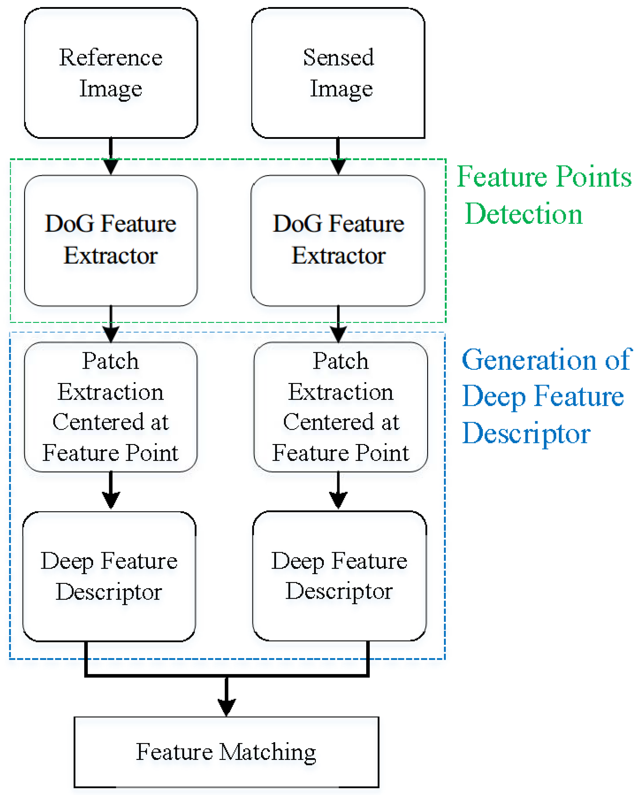
The procedure of the proposed method is presented in Figure 2 and it mainly contains four steps. The description of each step is as follows:
- (1)
- Feature detection. We utilized the known Difference of Gaussians (DoG) operator to detect the feature points in the reference and sensed images, respectively. The DoG algorithm was implemented by the vl_sift function from the open source computer vision tool, VLFeat [38]. All the parameters of DoG were the default values, including Octaves of 5, Levels of 3, FirstOctave of 0, EdgeThresh of 10, Magnif of 3 and WindowSize of 2. For each detected feature point, it had three corresponding ipieces of nformation, namely its location , scale and angle .
- (2)
- Image patch extraction. For each feature point, we extracted its surrounding area according to the detected scale and rotation angle, and then resampled to a pixels patch. Note that the radius of surrounding area was determined by the product of scale factor and constant number of . The extraction of image patch centered at the feature point was implemented by the vl_covdet function of VLFeat. The parameters descriptor, PatchResolution and PatchRelativeExtent of vl_covdet were ’patch’, 32 and 24, respectively.
- (3)
- Deep feature descriptor generation. We trained the deep convolutional network model using our created training samples from scratch, then utilized the trained model to generate descriptors for each feature point. The created training samples, structure of the model and how to train it were our major work, which will be detailed in the following.
- (4)
- Feature Matching. We matched the initial matching points based on the nearest Euclidean distance, then used Random Sampling Consensus (RANSAC) and transformed the model to eliminate the outlier further.In the initial matching based on the nearest neighbor, similarity research was implemented by the open source package fassi [39], developed by the Facebook AI research.
3.1. The Architecture of the Proposed Deep Convolutional Neural Network
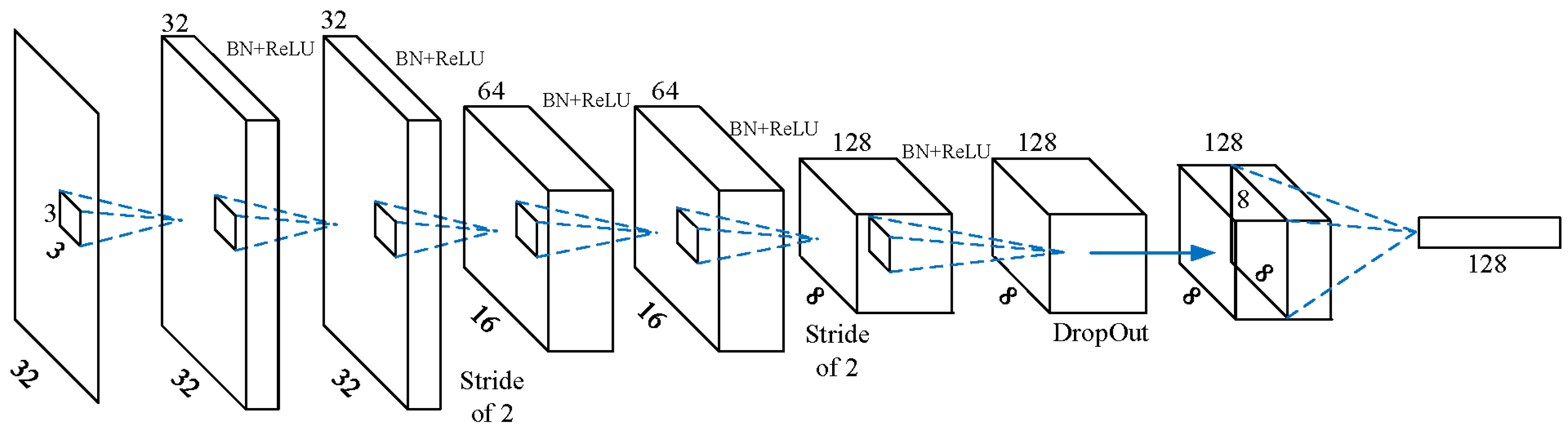
Among the comparison of image patches, the prevailing network is the Siamese network, which has two shared-parameters branches. However, its versatility is limited, especially for the feature point matching task. So, we adopted the non-Siamese network as our description network, named DescNet. The architecture of our network consisted of convolution layers, batch normalization layers, non-linear activation ReLU layers and 2-D dropblock layers [40]. All the convolution filters had the same small size of , except for the last convolution layer with the size of . The smaller size convolution kernel not only could reduce the number of parameters of network but also could increase the nonlinearity of network. Recently, many researchers found that the pooling layers decreased the performance of the output feature descriptor [41]. So, the shrinkage of feature map was implemented by increasing the stride of the convolution filter to two instead of carrying out the maxpooling operation. The architecture of model is shown in Figure 3. The details of each layer are presented in Table 1.
In Table 1, the format of output dimension is channel-first, namely (channel × height × width). Strides are only for convolution layers. Convolution layers are always padded with zeros such that their outputs are the same size as the input if the stride is one, or half of the size of input if the stride is two. All the convolution layers utilize the ReLU activation function and batch normalization operation except for the final layer, Conv6, whose output feature vector is normalized by the L2 Normalization function.
3.2. The Creation of Training Data
At present, there was no availability of public remote sensing patches for training a deep learning model to determine whether two patches were corresponding or not. However, manually extracting remote sensing patches and labeling them is a very time-consuming and tedious work. So, we proposed automatic method to extract the remote sensing patches and label them correctly. What’s more, considering the invariance of scale and angle of feature point, and motivated by the experience of hand-crafted descriptors, we extracted the corresponding patch of each point in the specific scale space and direction provided by the detected feature point. The basic process is consisted of five steps:
- (1)
- Selection of a pair of images. Two remote sensing scenes from the same area were selected, and one was divided into pixels tiles regularly. For each image tile with size of pixels, its corresponding tile was clipped from another scene according to the initial geographic coordinates.
- (2)
- Extraction of feature points. For each pair of images, the DoG detector was utilized to extract feature points. All the parameters of DoG were the default values, including Octaves of five, Levels of three, FirstOctave of zero, EdgeThresh of 10, Magnif of three and WindowSize of two. For each detected feature point, it had three corresponding pieces of information, namely its location , scale and angle .
- (3)
- Initial feature points matching. The SIFT descriptor and the nearest neighbor rule were utilized to acquire the initial matched feature points.
- (4)
- Refinement of initial matched points. The homograph transform model and random sample consensus (ransac) algorithm were introduced to further filter out false matched points.
- (5)
- The extraction of corresponding patches. For each pair of matched points, two surrounding area centered at two feature points were paired as a pair of corresponding patches. The extraction of image patch centered at the feature point was implemented by the vl_covdet function of VLFeat [38]. For each feature point detected by SIFT, its location information , scale information and angle information formed a column vector and then was passed as a parameter I to the function vl_covdet function to extract the image patch. For the parameters of descriptor, PatchResoultion and PatchRelativeExtent of vl_covdet function, they were “Patch”, 32 and 24, respectively.
It is worth noting that the dataset only includes the positive samples, namely corresponding patches. The negative samples, namely non-corresponding patches, can be generated online. The two patches from any two different points can be regarded as non-corresponding patches and the number of non-corresponding patches is much larger than the one of corresponding patches.
3.3. Training Strategy of Network
In the training phase, to ensure the full learning of training samples, we adopted the strategy of aggressively mining the ‘hardest’ negatives. In fact, for any training data set, the number of non-corresponding image patches was much larger than the number of corresponding image patches due to the fact that any two patches from different feature points could be paired as a non-corresponding patch. It was impossible to iterate all of the non-corresponding image patches. So, for an anchor patch, its corresponding patch was certain, and its non-corresponding patch was sampled randomly from the patches centered at other different feature points. According to the experiment findings, after a certain number of learning epochs, the network could reach a reasonable level of performance, but it had poor ability to determine the hard samples. To improve the performance further in the hard case, the strategy of aggressive mining of ‘hardest’ negatives was applied. The specific approach was at each epoch, and for the negative samples (non-corresponding patch pairs), we only kept the ‘hardest’ negatives, which had a smaller loss after forward-propagation through the network to update the weights of the network.
4. Experiments and Analysis
In each of the following experiments, except for special instructions, we utilized the same remote sensing training dataset for training the network and the same remote sensing test dataset for testing the performance of each method. For the training dataset, we generated a medium-scale of datasets, about 100,000 patches with size of pixels. They were from different sensors, such as GF-1, GF-2, ZY1-02C and ZY3, and they had different acquisition times, different resolutions and covered different ground objects.GF-1, GF-2, ZY1-02C and ZY3 were all from China. GF-1 and GF-2 were the first two of a series of high-resolution optical earth observation satellites of China National Space Administration. GF-1 was launched in 2013 and equipped with two scanners with 2 m resolution panchromatic and 8m resolution multispectral and four multispectral scanners with 16-m resolution. GF-2 was launched in 2014 and equipped with two scanners with 1 m panchromatic and 4 m high-resolution mulitspectral, respectively. ZY1-02C, launched on December 22, 2011 was equipped with multispectral scanner with 5 m and 10 m resolution multispectral images and panchromatic high-resolution scanner with 2.36 m panchromatic images. ZY3, launched on January 9, 2012 was equipped with front and rear scanner with 3.5 m resolution panchromatic images, a nadir scanner with 2.1 m resolution panchromatic image and a multispectral scanner with 6.0 m resolution multispectral images. The specific way of generation is detailed in the aforementioned Section 3.2. The training dataset is named as Invar-Dataset in the following. In the processing of training, the triplet margin loss function was utilized. It was defined about the triplets , where denotes anchor descriptor, denotes the positive descriptor and denotes the negative descriptor. Its expression is as follows:
where denotes the distance between anchor and positive descriptor, denotes the distance between anchor and negative descriptor, and is a predefined margin value. In our experiments, the value of was set to 1.0. The correct distance order should be . When the order was invalid, the loss function value was increased. In the process of training, the progressive reduction process of loss function guided the network to adjust its parameters to satisfy the order as much as possible. In the optimization method, Adam was applied to optimize the parameters of networks step by step. About the setting of related hyper-parameters for different methods, we tried to fine-tune them so that each method could get the best performance. Their concrete values were reported in the following experiments. Training was done with PyTorch library [42].
4.1. The Qualitative Evaluation of the Proposed DescNet
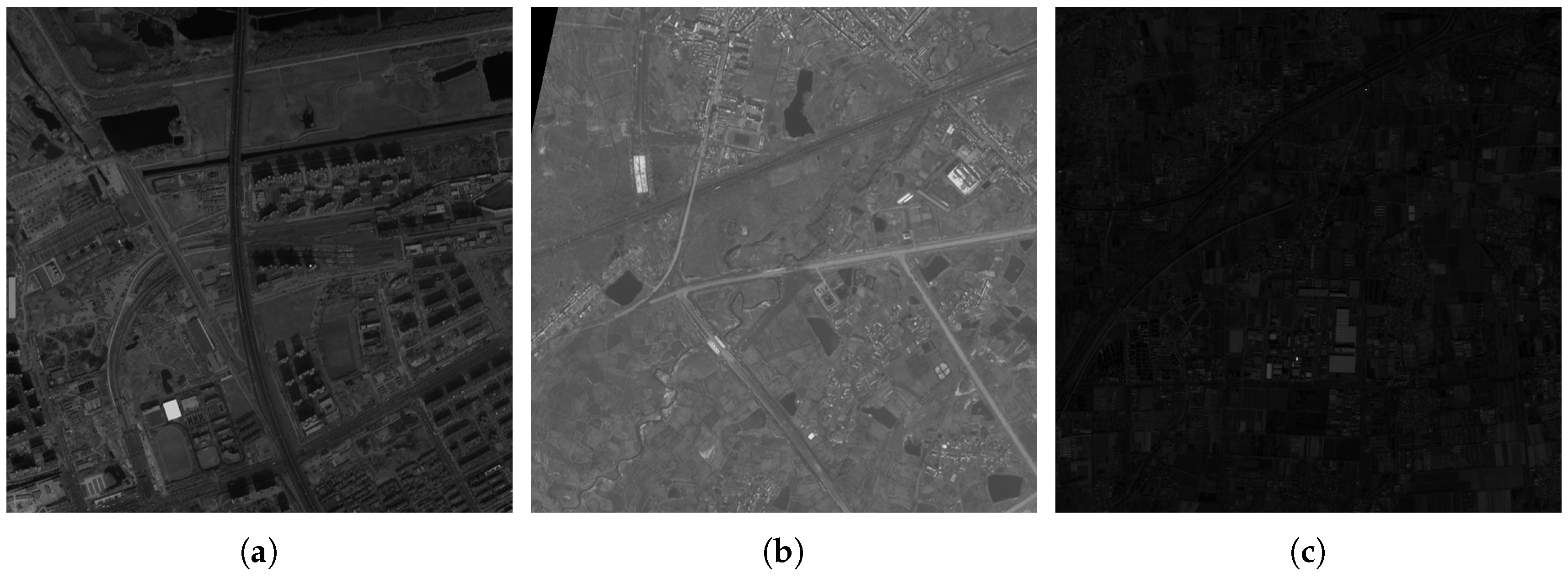
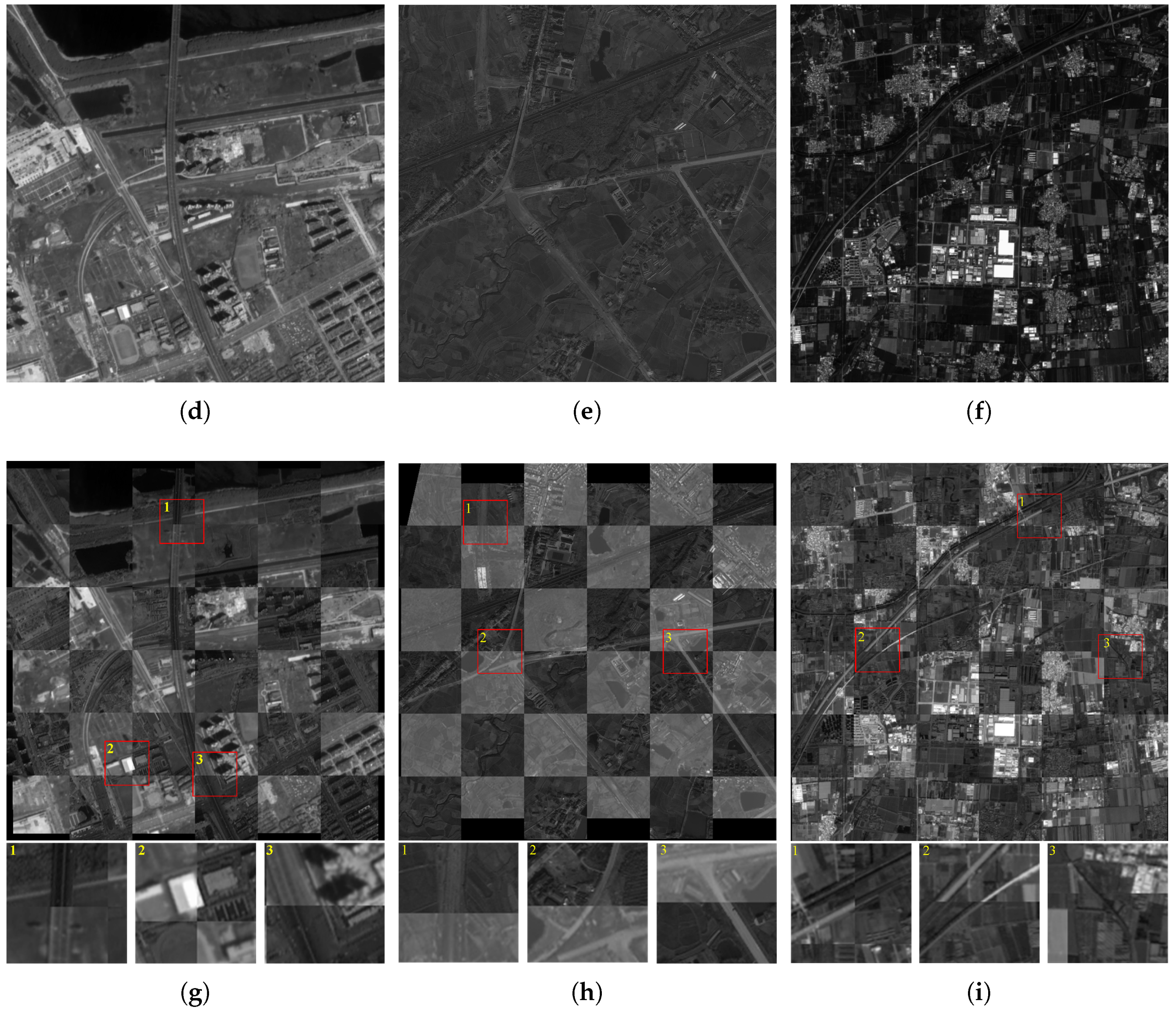
To validate the effectiveness of the proposed DescNet, we utilized the feature descriptor generated by DescNet to register remote sensing images. Three pairs of images were applied to test. The three pairs of remote sensing images are shown in Figure 4. Their metadata information was summarized in Table 2.
The DescNet was trained from the created remote sensing image sets, while Invar-Dataset was trained from scratch. The initial learning rate was set to , and the strategy of decaying was setting the learning rate to the initial value decayed by gamma every epoch. The gamma was set to 0.99. The total training epochs were 1000 epochs. After finishing the training task, we utilized the trained DescNet to generate a feature description vector for each feature point detected by vl_sift [38] from each pair of images. The initial matching criterion was the nearest Euclidean distance and then these initial matched points were further refined by the condition that the nearest Euclidean distance multiplied by the thresh was no longer greater than the distance to other feature vectors. The thresh was set to 1.5. After acquiring the corresponding points, the homography transform model and RANSAC algorithm were applied to rectify the sensed image. To illustrate the registration results clearly, the checkerboard visualization of reference and rectified images are shown in Figure 4.
From Figure 4, we can see that all the registration results are satisfied by carefully observing the alignment of distinctive features circled by the red ellipses. In fact, these image pairs have great grayscale difference and content changes. The content of image pair01 underwent some changes and the images in the image pair02 had large grayscale difference. For image pair03, besides the huge grayscale difference, the type of Sentinel-2 remote sensing images were not included in the training datasets. This shows that the DescNet has good generalization ability and was able to generate robust descriptors for remote sensing image feature matching.
4.2. The Superiority of Different Training Datasets
To validate the superiority of our created training data, Invar-Dataset, and to show that it is beneficial for a deep convolutional network to learn good descriptors of feature points from remote sensing images in practical applications, we created another set of remote sensing training data in a different way. The main difference was the way of the extraction of patch for each feature point. For two remote sensing scenes, one was resampled to the same resolution as the other one, then the patch for each feature point was extracted from the original or resampled image directly with no further processing of rotation or scaling. The training dataset was named as Orig-Dataset. The proposed deep convolutional neural network, DescNet, was trained from these two-different training datasets from scratch, respectively. The initial learning rate of Adam optimization algorithm was . As for the decay strategy of learning rate, we set the learning rate to the initial value decayed by gamma every epoch. The value of gamma was set to 0.99. The total training epoch was 1000 epochs. Here, we evaluated the superiority of our created dataset from two aspects. One was from the classification benchmark test due to the matching problem that can be formulated as a classification problem, the other was from the feature points matching test due to the feature points matching our final target.
4.2.1. The Classification Benchmark Test
In the classification benchmark test, we evaluated the performance of DescNet trained from different training datasets Invar-Dataset, Orig-Dataset in determining whether two patches were corresponding or not. The respective test dataset was created in the same way as the creation of their respective training dataset. Specially, the non-corresponding patches were from the false matched points which are determined by the SIFT descriptor. The number of corresponding and non-corresponding patches was equal, with both of them being 10,813 pairs. The metrics of average precision (AP), area under curve (AUC) and fpr80 (false positive rate at point of 0.80 true positive recall) are reported in the Table 3.
For the AUC and AP, the larger they were, the better the network performed. They both had an ideal value of 1. For the FPR80, the smaller it was, the better the network performed. Its ideal value was 0. From the Table 3, we can see that all the metrics of AUC, AP and FPR80 of the network trained using Invar-Dataset were slightly superior to the corresponding ones of network trained using Orig-Dataset. Only from the classification benchmark, it is hard to draw a conclusion that Invar-Dataset is superior to Orig-Data. In fact, this is because the classification benchmark does not really reflect the nearest neighbor matching, which is consistent with the founding in [31].
4.2.2. The Feature Points Matching Test
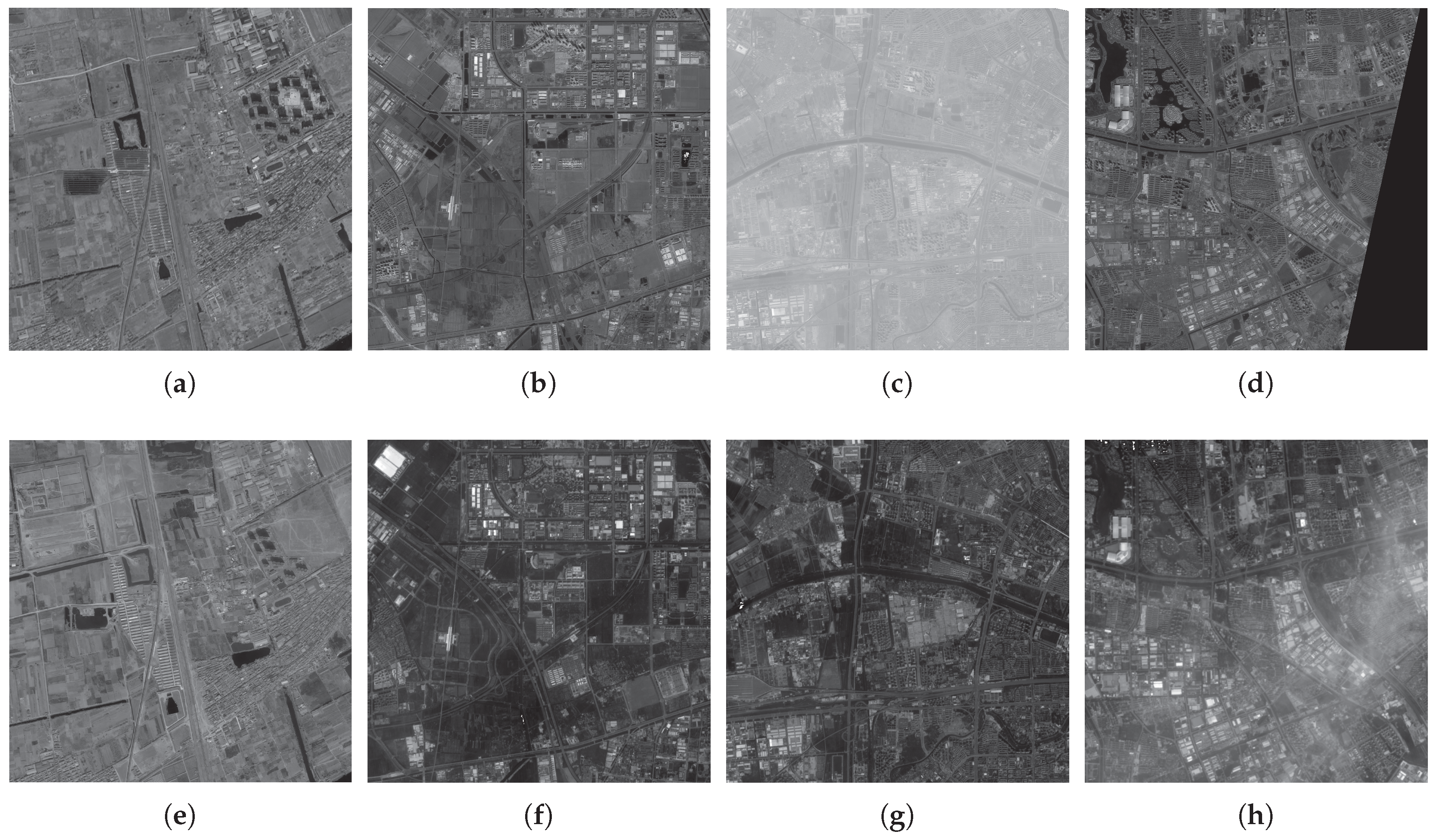
In the feature points matching test, the test remote sensing images, GF-1 and GF-2 remote sensing images were applied. The content covered by the images was diverse, including man-made buildings, mountains, farmland and so on. For some image pairs, they had different acquisition times, so some content may have changed or have been occluded by cloud, and they had a large gray difference. So, the generation of a good descriptor for each feature point was a very challenging task. There were 173 pairs of test images with the same size of pixels in total. Among them, four pairs of samples were shown in Figure 5, and their corresponding metadata information is summarized in Table 4. We first used vl_sift algorithm to detect the feature points, and then extracted their corresponding patch with the size pixels in the same way as in the creation of their training data. For each patch, we first resized it to satisfy the input size requirement of network, then fed it into the network, and acquired the 128-deminsion feature vector in the final. For each feature vector, we found its nearest neighbor feature vector as its matching one according to the metrics of Euclidean distance. To reject matches that were too ambiguous, we utilized the criterion suggested by D. Lowe [20] that the smallest distance multiplied by thresh was not greater than the distance to other feature vectors. The value of thresh was set to 1.5. Note that the feature vector was normalized to unit length. After achieving the initial corresponding points, we then utilized the homography model and RANSAC (random sample consensus) algorithm to refine these feature points. For RANSAC algorithm, the number of iteration was set to 1000. Finally, when the distance error of corresponding points was less than 2.0 pixels, they were regarded as a pair of correctly matched points. For the DescNet, trained from different training dataset, the average number of matched points of each pair of images iss reported in Table 5, respectively. At the same time, the Root Mean Square Error in the x and y direction , and the overall Root Mean Square Error, for matched points are also reported in Table 5. The calculation of , and is calculated as follows: , , , where (,) denotes the coordinates of matched points in the transformed image, (,) denotes the coordinates of matched points in the reference image. N denotes the total number of matched points.
From Table 5, we can see that the average number of achieved matched feature points of DescNet trained from Invar-Dataset is larger than the one of DescNet trained from Orig-Dataset significantly. At the same time, in terms of the coordinate error metrics of , and , their differences are very small. This shows that compared to Orig-Dataset, our created training dataset is more beneficial for deep convolutional network to learn a good feature descriptor for point matching in remote sensing image registration. What’s more, there is almost no additional cost to create the Invar-Dataset because the detected feature point has the corresponding scale and orientation information. Besides, the advantage is easy to understand, because when the raw patch of feature point fed into the network, it had to be further processed by the different convolution filters to try to achieve the invariance of scale and orientation, while the patch of feature point extracted from the detected scale space and orientation carried the scale and orientation information which had proved to be effective for the conventional hand-designed descriptor. So, for the simple architecture of network, such as DescNet, it is difficult to get an output of robust feature descriptor vector from a raw input patch. Maybe for the more complicated architecture of network, such as the multi-pyramid feature network [43], a good feature descriptor can be generated from the raw input patch. Certainly, the training and prediction cost would raise dramatically.
4.2.3. The Rotation Invariance of Invar-Dataset
To test the rotation invariance of Invar-Dataset more explicitly, we randomly rotated the same 173 pairs of test images as utilized in the aforementioned feature points matching Section 4.2.2. The rotation angle range was from to . The experiment evaluation process for the rotated 173 paris of images was the same as the aforementioned experiment. Here, we called the aforementioned feature points matching as the non-rotated test, and called this experiment the rotated test. For the DescNet trained from Invar-Dataset, its performance on the rotated test and non-rotated test were reported in Table 6. By comparing the experiment results of the Non-rotated test and rotated test, we can roughly draw a conclusion that the DescNet trained from Invar-Dataset has the property of rotation invariance. As for the average correct number of matched points of the rotated test, it was slightly lower than the one of non-rotated test. We think this is reasonable, because the accuracy of principle orientation of the SIFT descriptor was not very high. However, for the DescNet trained from Orig-Dataset, it failed to acquire the corresponding points for 150 pairs of the 173 pairs of test images, and the average number of correct corresponding points for the 23 pairs of test images was less than 22.5. This shows that our created Invar-Dataset had rotation invariance, while Orig-Dataset was sensitive to rotation.
4.3. The Comparison of Performance of Different Architectures of Network
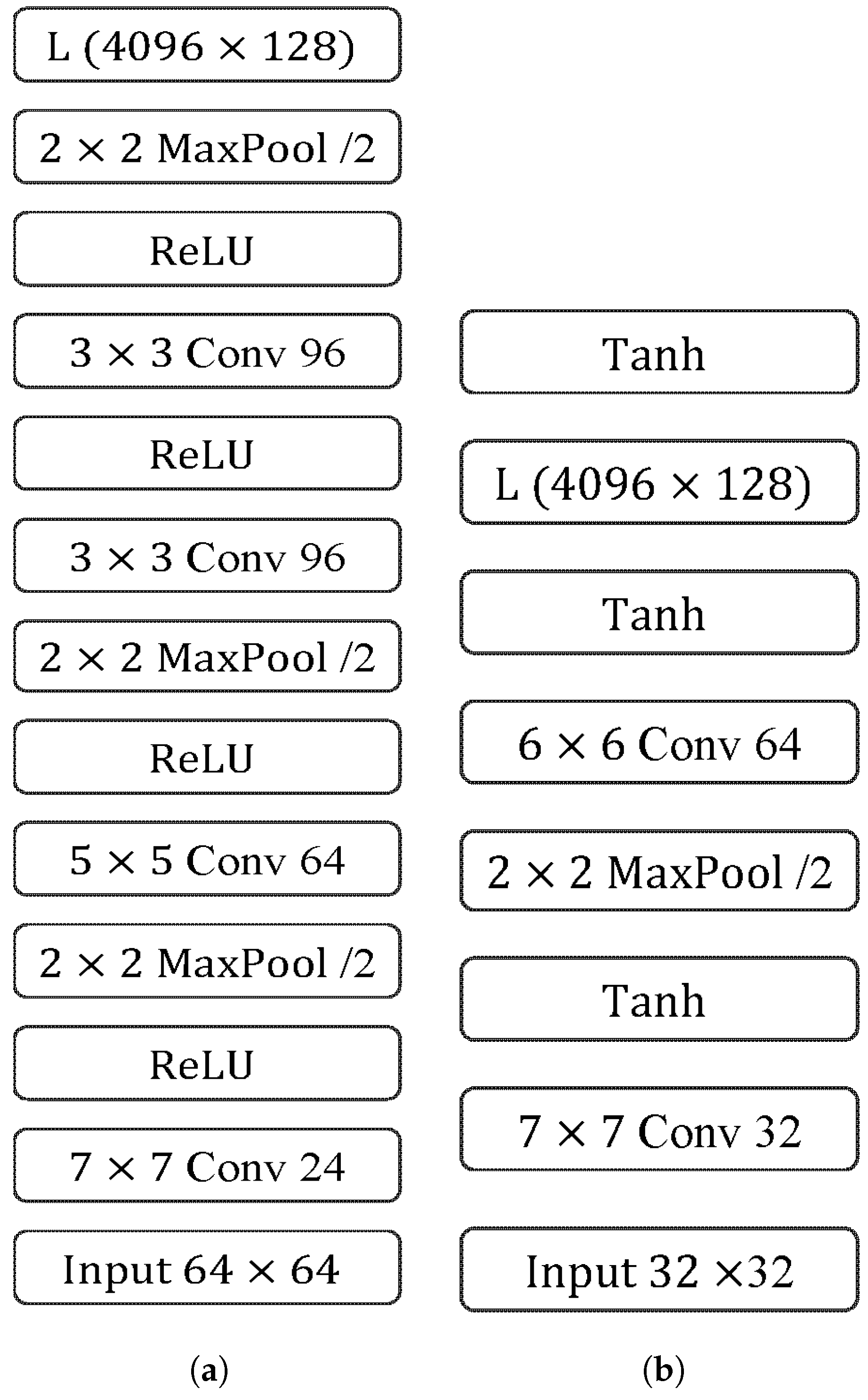
In this section, to validate the performance of our network, DescNet, we compared our network to two other popular networks, the TFeat [31] and MatchNet [25] networks, the most popular conventional, hand-crafted SIFT descriptors. MatchNet was essentially a Siamese-Network, and consisted of three subnetworks, namely, a feature extraction network, a bottleneck network and a metric network. For a fair comparison, we only adopted its feature extraction network to compare. Its feature extraction network was composed of five convolution layers, and the first two convolution filters size were and , respectively, and the last three convolution filters size were all . The shrinkage of feature map was implemented by the operation of maxpooling. Its input patch size was and the final output feature vector was also a 128-dimension vector. Its architecture schema is shown in Figure 6a. The TFeat network consisted of two convolution layers, whose filters size were and , respectively, with one linear layer and one non-linear activation Tanh layer. Its input patch size was and output feature vector was also a 128-dimension vector. Its architecture schema is shown in Figure 6b. For the SIFT descriptor, it was generated by the algorithm vl_sift provided by the vl_feat toolbox [38].
For all the three different networks, we utilized the same train data, invar-Dataset to train them. In the specific training process of each network, we fine-tuned all the hyperparameters, including the parameters of optimization method, and training epochs to achieve the most optimal performance. The initial learning rate for TFeat, MatchNet and DescNet was , and , respectively. As for the decay strategy of learning rate, we set the learning rate to the initial value decayed by gamma every epoch. The gamma value for the TFeat, MatchNet and DescNet were 0.99, 0.99 and 0.999, respectively. Both DescNet and MatchNet were trained for 1000 epochs, and TFeat was trained for 1200 epochs.
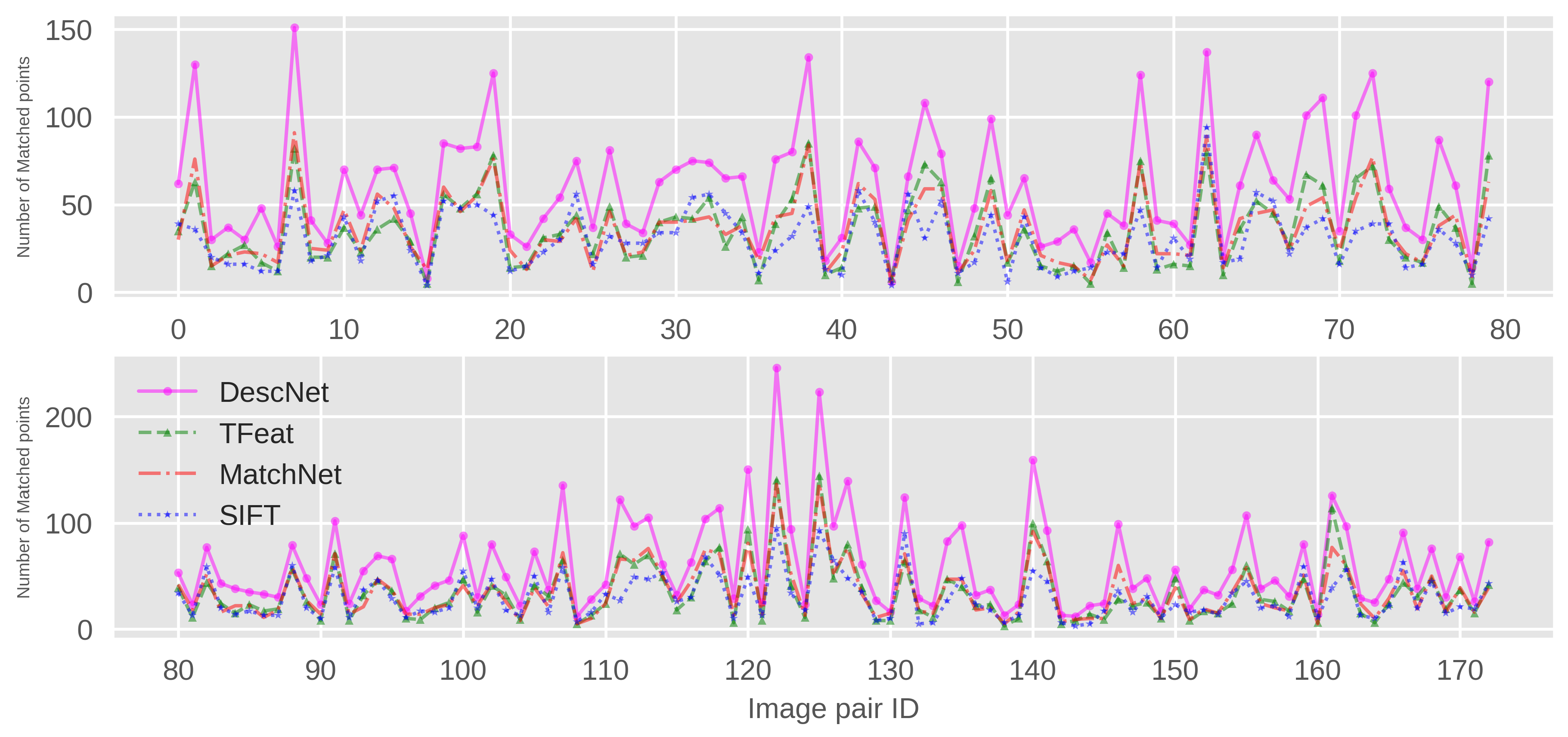
For testing the performance of different methods, we used the same test remote sensing images as in the feature points matching experiment in the Section 4.2.2. The same measurements , and were utilized to evaluate the performance of the deep convolutional networks with different architectures. The inlier ratio was the ratio of correct matched point to the initial corresponding points. The experiment results were reported in Table 7. At the same time, we also reported the number of the acquired corrected matched point for each pair of image for four different methods, as shown in Figure 7.
From Figure 7, we can see that the proposed matching network, DescNet, acquired the most matched points for each image among these methods. For the other three methods, TFeat, MatchNet and SIFT, it was hard to rank them in terms of the acquired number of matched points. From Table 7, we can see that DescNet almost received twice as many matched points as the SIFT method, and much more matched points than TFeat and MatchNet. The TFeat, MatchNet and SIFT acquired similar amounts of matched points. From the view of average inlier ratio, DescNet had better performance in determining the matched points than other methods. Due to the unknown nature of true transform models, it is hard to evaluate the accuracy of image registration. But from the aspect of the number of inliers, the transform model estimated that the DescNet acquired most supported features, which shows that DescNet has the better ability in determining the corresponding points. As for the error measurements of , and , they represent the geometric inconsistency (fitting error) of estimated transform model. Although DescNet almost acquired the maximum error, compared to the corresponding minimum error, the gap was very minor, and the largest gap was about 0.05 pixels, in the level of pixels. In fact, the comparison of error measurements of different methods were not important as long as the error are reasonably small. As for why DescNet didn’t get a smaller coordinates error of matched points, it may be resulted from the location error of feature detector DoG, or the different number of matched points.
4.4. The Generality of DescNet
For deep learning, the generality of trained network was also a key issue. In our experiment, we utilized remote sensing images from China areas to train the proposed network DescNet. To validate whether the trained network could be applied to remote sensing images from other countries in the world, we selected another 20 pairs of Google Earth remote sensing images from America, Brazil, Germany and Australia to test the performance of DescNet. Four samples of them were shown in Figure 8, and their metadata were given in Table 8. The experimental process was the same as the the feature points matching test Section 4.2.2. The performance of DescNet trained from Invar-Dataset on the 20 pairs of Google Earth test images was reported in Table 9.
From the measurement of , , and inlier ratio, the DescNet could be applied to the remote sensing images from other countries, although the training data, Invar-Dataset, were all from China regions. This showed that DescNet has a good generality of the different locations of images. In fact, it is also very easy to understand this because the feature extraction and feature description was a low-level computer vision task, compared to object recognition and image understanding, and only a small surrounding area of feature point was utilized to generate the descriptor. At the same, the dropout layer of DescNet could also prevent the overfitting.
5. Discussion
5.1. The Analysis of Effectiveness of DescNet for Image Registration
In the experiment section, we first qualitatively illustrated the effectiveness of DescNet for remote sensing images registration by means of the checkerboard visualization. The experimental remote sensing data were very challenging as they underwent content changes and large grayscale difference. Moreover, the DescNet could be utilized to register Sentinel-2 image, which was not presented in the training data. This illustrated that the trained DescNet had a good generalization capacity and could be utilized to replace hand-designed descriptor for the practical remote sensing image registration.
5.2. The Analysis of Superiority of Training Dataset
For our created training dataset, Invar-Dataset, not only were they able to be created automatically, but they could also make DescNet learn a good descriptor of feature points from an image pair with scale and angle difference. There is no doubt that the automatic creation of training samples can promote the application of DescNet in the practical and large-scale registration applications. For the merit of enabling DescNet to learn a good descriptor of feature points from an image pair with scale and angle difference, another training dataset of Orig-Dataset was utilized to train the same network, DescNet. Performance evaluation was performed in a classification benchmark test and feature points matching test. In the evaluation of classification benchmark, the measurements of AP, AUC and FPR80 were all similar, and the advantage of Invar-Dataset was small. However, in the feature points matching, the DescNet trained from Invar-Dataset achieved a larger number of matched points than DescNet trained from Orig-Dataset. We also validated the rotation invariance of DescNet trained from Invar-Dataset. However, for the DescNet trained from Orig-Dataset, it was very sensitive to image rotation. In fact, the difference in the evaluation results is that the classification benchmark was not a representative measure for the practical application of feature points matching [31]. So, the created training dataset of Invar-Dataset is more suitable for training DescNet for image registration.
5.3. The Analysis of Architecture of DescNet
To demonstrate the advantage of the proposed Network of DescNet, we compared two other convolution networks TFeat and MatchNet, and one conventional and representative descriptor SIFT. The experiment results show that DescNet had a large superiority in matching corresponding points than the other two networks and SIFT method. For MatchNet, the size of convolutional filters were different, including , and , and the special pooling layers were utilized to reduce the size of feature map. While for DescNet, it had a smaller size of convolution filters (all the convolution filters have the same size of ), and the shrinkage of feature map was implemented by setting the stride of convolution filters to two. The evolution from the architecture of MatchNet to the one of DescrNet was based on the recent experience of designing network architecture for better performance in many computer vision tasks, such as VGGNet and ResNet. This shows that for the generation of a descriptor of feature points, fine-grained features (captured by the smaller size of convolution filter) were more important. The replacement of pooling layer by convolution layer with strides of two could reduce the loss of feature map and was also beneficial for generating a good feature descriptor. Compared to DescNet, the characteristics of TFeat, including a shallow network, a larger size of convolution filter and usage of pooling layer resulted in its worse performance. However, for the comparison between TFeat and MatchNet, although the layer of MatchNet was much deeper, its performance barely improved. It shows that, for the feature descriptor generation, the appropriate component of network was more important than simply stacking more layers.
5.4. The Further Analysis of DescNet
In the training phase of DescNet, we tried different loss functions and the existing public natural image patch datasets, HPatches to give more insights.
As for loss function, we tried to use the contrastive loss, as expressed in Formula (1). The experimental results show that, for all the networks of TFeat, MatchNet and DescNet, in terms of number of correctly matched points, the performance of network trained with contrastive loss was worse than the one of network trained with triplet margin loss. This shows that triplet margin loss function is more suitable to the task of feature descriptor vector generation. Actually, the triplet margin loss considered the positive and negative samples together, and the dynamic mining of hard negative samples in the triplet margin loss was also beneficial to the final improvement of performance.
As for the usage of the existing public natural image patches, HPatches, we tried to utilize the transfer learning technology, namely first trained DescNet using HPatches from scratch, then fine-tuned the pre-trained DescNet using our created remote sensing dataset, Invar-Dataset. In the process of the experiment, we found that the acquired number of correctly matched points of DescNet trained from HPatches and Invar-Dataset basically was equal to the one of DescNet trained only from Invar-Dataset. But the pretrained DescNet from HPatches could accelerate the training from Invar-Dataset, which shows that there exists a certain degree of similarities between the domain of natural images and the one of remote sensing. As for there iwas no improvement in final performance, we think the number and diversity of Invar-Dataset was large enough for the testing images, and the deformation of remote sensing image pairs were not very complicated after corrected by the initial imaging model, compared to shear and reverse deformation.
6. Conclusions
In this paper, we proposed a novel way of creating training samples automatically, which makes deep learning possible for feature matching of remote sensing images. Then we utilized the learned descriptor vector generated by a deep convolutional network of DescNet to replace the hand-designed feature description vector. This replacement can increase the number of correct matched points in the task of remote sensing image registrations significantly, even for different remote sensing images with different resolutions, large grayscale differences and so on. This proved that the DescNet can generate a better and more robust feature description vector for feature point, which has a better ability to determine the matched points. To validate the superiority of our created dataset Invar-Dataset, another training dataset Orig-Dataset was created, and the performance comparison of the same network trained from these two different training datasets was analyzed. Experiment results illustrated that Invar-Dataset can promote the neural network to generate a more better, robust feature descriptor. To validate the superiority of the proposed network, DescNet, we carried out qualitative and quantitative experiments. In the qualitative experiments, we illustrated the effectiveness of DescNet in image registration by means of checkerboard visualization. In the quantitative experiments, we compared it with other two networks, TFeat and MatchNet and one conventional hand-crafted feature description algorithm, SIFT. The experimental results showed that the DescNet can acquire significantly more correct matched points than other three methods, and at the same time the coordinate error is almost the same. So, the network DescNet trained from Invar-Dataset can be regarded as a good feature descriptor for remote sensing image features matching.
In the evaluation of performance of the network, although determining whether two feature points are corresponding can be naturally formulated as a classification problem, our experimental results showed that the classification benchmark is not a representative measure for the real-world feature points matching. So, in the future, we should not only pay attention to the curve of classification indicators during training, but also consider the measurements in the practical feature points matching, which may help to train a better network.
Author Contributions
Y.D. developed the methods, carried out the experiments and wrote the manuscripts. W.J. and T.L. supervised the research. All the authors analyzed the results and improved the manuscript.
Funding
This research was funded by the program of the National Natural Science Foundation of China (61731022 and 61701495); the Strategic Priority Research Program of the Chinese Academy of Sciences (XDA19090300) and the National Key Research and Development Programs of China (2016YFA0600302).
Conflicts of Interest
The authors declare no conflict of interest.
References
- Newsam, S.; Yang, Y. Comparing global and interest point descriptors for similarity retrieval in remote sensed imagery. In Proceedings of the 15th Annual ACM International Symposium on Advances in Geographic Information Systems, Seattle, WA, USA, 7–9 November 2007; p. 9. [Google Scholar]
- Philbin, J.; Chum, O.; Isard, M.; Sivic, J.; Zisserman, A. Object retrieval with large vocabularies and fast spatial matching. In Proceedings of the CVPR’07 IEEE Conference on Computer Vision and Pattern Recognition, Minneapolis, MN, USA, 17–22 June 2007; pp. 1–8. [Google Scholar]
- Cheng, G.; Han, J. A survey on object detection in optical remote sensing images. ISPRS J. Photogramm. Remote Sens. 2016, 117, 11–28. [Google Scholar] [CrossRef] [Green Version]
- Fergus, R.; Perona, P.; Zisserman, A. Object class recognition by unsupervised scale-invariant learning. In Proceedings of the 2003 IEEE Computer Society Conference on Computer Vision and Pattern Recognition, Madison, WI, USA, 18–20 June 2003; p. II. [Google Scholar]
- Liu, X.; Ai, Y.; Zhang, J.; Wang, Z. A novel affine and contrast invariant descriptor for infrared and visible image registration. Remote Sens. 2018, 10, 658. [Google Scholar] [CrossRef]
- Liu, Y.; Mo, F.; Tao, P. Matching Multi-Source Optical Satellite Imagery Exploiting a Multi-Stage Approach. Remote Sens. 2017, 9, 1249. [Google Scholar] [CrossRef]
- Yang, K.; Pan, A.; Yang, Y.; Zhang, S.; Ong, S.H.; Tang, H. Remote sensing image registration using multiple image features. Remote Sens. 2017, 9, 581. [Google Scholar] [CrossRef]
- Wang, X.; Li, Y.; Wei, H.; Liu, F. An ASIFT-based local registration method for satellite imagery. Remote Sens. 2015, 7, 7044–7061. [Google Scholar] [CrossRef]
- Sugimoto, R.; Kouyama, T.; Kanemura, A.; Kato, S.; Imamoglu, N.; Nakamura, R. Automated Attitude Determination for Pushbroom Sensors Based on Robust Image Matching. Remote Sens. 2018, 10, 1629. [Google Scholar] [CrossRef]
- Kouyama, T.; Kanemura, A.; Kato, S.; Imamoglu, N.; Fukuhara, T.; Nakamura, R. Satellite attitude determination and map projection based on robust image matching. Remote Sens. 2017, 9, 90. [Google Scholar] [CrossRef]
- Oliveira, F.P.; Tavares, J.M.R. Medical image registration: A review. Comput. Methods Biomech. Biomed. Eng. 2014, 17, 73–93. [Google Scholar] [CrossRef] [PubMed]
- Viola, P.; Wells, W.M., III. Alignment by maximization of mutual information. Int. J. Comput. Vis. 1997, 24, 137–154. [Google Scholar] [CrossRef]
- Dong, Y.; Long, T.; Jiao, W.; He, G.; Zhang, Z. A novel image registration method based on phase correlation using low-rank matrix factorization with mixture of Gaussian. IEEE Trans. Geosci. Remote Sens. 2018, 56, 446–460. [Google Scholar] [CrossRef]
- Dasgupta, B.; Chatterji, B. Fourier-mellin transform based image matching algorithm. IETE J. Res. 1996, 42, 3–9. [Google Scholar] [CrossRef]
- Dong, Y.; Jiao, W.; Long, T.; He, G.; Gong, C. An Extension of Phase Correlation-Based Image Registration to Estimate Similarity Transform Using Multiple Polar Fourier Transform. Remote Sens. 2018, 10, 1719. [Google Scholar] [CrossRef]
- He, H.; Chen, M.; Chen, T.; Li, D. Matching of Remote Sensing Images with Complex Background Variations via Siamese Convolutional Neural Network. Remote Sens. 2018, 10, 355. [Google Scholar] [CrossRef]
- Sedaghat, A.; Mokhtarzade, M.; Ebadi, H. Uniform robust scale-invariant feature matching for optical remote sensing images. IEEE Trans. Geosci. Remote Sens. 2011, 49, 4516–4527. [Google Scholar] [CrossRef]
- Sedaghat, A.; Ebadi, H. Remote sensing image matching based on adaptive binning SIFT descriptor. IEEE Trans. Geosci. Remote Sens. 2015, 53, 5283–5293. [Google Scholar] [CrossRef]
- Sedaghat, A.; Ebadi, H. Accurate affine invariant image matching using oriented least square. Photogramm. Eng. Remote Sens. 2015, 81, 733–743. [Google Scholar] [CrossRef]
- Lowe, D.G. Distinctive image features from scale-invariant keypoints. Int. J. Comput. Vis. 2004, 60, 91–110. [Google Scholar] [CrossRef]
- Zou, Q.; Ni, L.; Zhang, T.; Wang, Q. Deep Learning Based Feature Selection for Remote Sensing Scene Classification. IEEE Geosci. Remote Sens. Lett. 2015, 12, 2321–2325. [Google Scholar] [CrossRef]
- He, K.; Zhang, X.; Ren, S.; Sun, J. Deep residual learning for image recognition. In Proceedings of the IEEE Conference on Computer Vision and Pattern Recognition, Las Vegas, NV, USA, 27–30 June 2016; pp. 770–778. [Google Scholar]
- Badrinarayanan, V.; Kendall, A.; Cipolla, R. Segnet: A deep convolutional encoder-decoder architecture for image segmentation. arXiv, 2015; arXiv:1511.00561. [Google Scholar] [CrossRef]
- Gordo, A.; Almazán, J.; Revaud, J.; Larlus, D. Deep image retrieval: Learning global representations for image search. In Proceedings of the European Conference on Computer Vision, Amsterdam, The Netherlands, 8–16 October 2016; Springer: Berlin, Germany, 2016; pp. 241–257. [Google Scholar]
- Han, X.; Leung, T.; Jia, Y.; Sukthankar, R.; Berg, A.C. Matchnet: Unifying feature and metric learning for patch-based matching. In Proceedings of the IEEE Conference on Computer Vision and Pattern Recognition, Boston, MA, USA, 7–12 June 2015; pp. 3279–3286. [Google Scholar]
- Tian, Y.; Fan, B.; Wu, F. L2-Net: Deep Learning of Discriminative Patch Descriptor in Euclidean Space. In Proceedings of the 2017 IEEE Conference on Computer Vision and Pattern Recognition (CVPR), Honolulu, HI, USA, 21–26 July 2017; Volume 1, p. 6. [Google Scholar]
- Tola, E.; Lepetit, V.; Fua, P. Daisy: An efficient dense descriptor applied to wide-baseline stereo. IEEE Trans. Pattern Anal. Mach. Intell. 2010, 32, 815–830. [Google Scholar] [CrossRef]
- Dimitrovski, I.; Kocev, D.; Kitanovski, I.; Loskovska, S.; Džeroski, S. Improved medical image modality classification using a combination of visual and textual features. Comput. Med. Imaging Gr. 2015, 39, 14–26. [Google Scholar] [CrossRef] [PubMed]
- Ioffe, S.; Szegedy, C. Batch normalization: Accelerating deep network training by reducing internal covariate shift. arXiv, 2015; arXiv:1502.03167. [Google Scholar]
- Mishchuk, A.; Mishkin, D.; Radenovic, F.; Matas, J. Working hard to know your neighbor’s margins: Local descriptor learning loss. In Advances in Neural Information Processing Systems; MIT Press: Cambridge, MA, USA, 2017; pp. 4826–4837. [Google Scholar]
- Balntas, V.; Riba, E.; Ponsa, D.; Mikolajczyk, K. Learning Local Feature Descriptors With Triplets and Shallow Convolutional Neural Networks. In Proceedings of the British Machine Vision Association (BMVC) 2016, York, UK, 19–22 September 2016; Volume 1, p. 3. [Google Scholar]
- Xie, J.; He, T.; Zhang, Z.; Zhang, H.; Zhang, Z.; Li, M. Bag of Tricks for Image Classification with Convolutional Neural Networks. arXiv, 2018; arXiv:1812.01187. [Google Scholar]
- Snavely, N.; Seitz, S.M.; Szeliski, R. Photo tourism: Exploring photo collections in 3D. In ACM Transactions on Graphics (TOG); ACM: New York, NY, USA, 2006; Volume 25, pp. 835–846. [Google Scholar]
- Balntas, V.; Lenc, K.; Vedaldi, A.; Mikolajczyk, K. HPatches: A benchmark and evaluation of handcrafted and learned local descriptors. In Proceedings of the Conference on Computer Vision and Pattern Recognition (CVPR), Honolulu, HI, USA, 21–26 July 2017; Volume 4, p. 6. [Google Scholar]
- Zagoruyko, S.; Komodakis, N. Learning to compare image patches via convolutional neural networks. In Proceedings of the IEEE Conference on Computer Vision and Pattern Recognition, Boston, MA, USA, 7–12 June 2015; pp. 4353–4361. [Google Scholar]
- Schroff, F.; Kalenichenko, D.; Philbin, J. Facenet: A unified embedding for face recognition and clustering. In Proceedings of the IEEE Conference on Computer Vision and Pattern Recognition, Boston, MA, USA, 7–12 June 2015; pp. 815–823. [Google Scholar]
- Hoffer, E.; Ailon, N. Deep metric learning using triplet network. In International Workshop on Similarity-Based Pattern Recognition; Springer: Berlin, Germany, 2015; pp. 84–92. [Google Scholar]
- Vedaldi, A.; Fulkerson, B. VLFeat: An open and portable library of computer vision algorithms. In Proceedings of the 18th ACM International Conference on Multimedia, Firenze, Italy, 25–29 October 2010; pp. 1469–1472. [Google Scholar]
- Johnson, J.; Douze, M.; Jégou, H. Billion-scale similarity search with gpus. arXiv, 2017; arXiv:1702.08734. [Google Scholar]
- Ghiasi, G.; Lin, T.Y.; Le, Q.V. DropBlock: A regularization method for convolutional networks. In Advances in Neural Information Processing Systems; MIT Press: Cambridge, MA, USA, 2018; pp. 10748–10758. [Google Scholar]
- Springenberg, J.T.; Dosovitskiy, A.; Brox, T.; Riedmiller, M. Striving for simplicity: The all convolutional net. arXiv, 2014; arXiv:1412.6806. [Google Scholar]
- Pytorch. Available online: https://pytorch.org/ (accessed on 1 January 2019).
- Lin, T.Y.; Dollár, P.; Girshick, R.B.; He, K.; Hariharan, B.; Belongie, S.J. Feature Pyramid Networks for Object Detection. In Proceedings of the 2017 IEEE Conference on Computer Vision and Pattern Recognition (CVPR), Honolulu, HI, USA, 21–26 July 2017; Volume 1, p. 4. [Google Scholar]
Figure 1.
(a) is the structure of the Siamese Network, it has two branch networks and they have the tied parameters. Its output is the probability of patch correspondence. (b) is the structure of non-Siamese Network, it has a single branch network, which is played as feature encoder. Its output is a 1-D feature vector.

Figure 2.
The procedure of the proposed method.

Figure 3.
The architecture of DescNet.

Figure 4.
For each column, the top two rows are reference and sensed images, the bottom row is a checkerboard visualization of corrected images. Take image (g) as an example, the area defined by a red square with yellow label number is enlarged to display in the square image with the same label number for clear visualization. The same rule applies to image (h,i). In particular, for a clear visual presentation, the square root method was applied to stretch the grayscale of image (i).


Figure 5.
Four samples of test remote sensing images. Each column is a pair of images. Image pair of (a,e) underwent image content changes, image pair of (b,f) and image pair of (c,g) had great gray difference, image pair of (d,h) underwent occlusion by cloud.
Figure 5.
Four samples of test remote sensing images. Each column is a pair of images. Image pair of (a,e) underwent image content changes, image pair of (b,f) and image pair of (c,g) had great gray difference, image pair of (d,h) underwent occlusion by cloud.

Figure 6.
The architectures of the different networks MatchNet and TFeat. (a) is the architecture of MatchNet and (b) is the architecture of TFeat.
Figure 6.
The architectures of the different networks MatchNet and TFeat. (a) is the architecture of MatchNet and (b) is the architecture of TFeat.

Figure 7.
The acquired number of matched points of each image pair for four different methods, DescNet, TFeat, MatchNet and Scale Invariant Feature Transform (SIFT).
Figure 7.
The acquired number of matched points of each image pair for four different methods, DescNet, TFeat, MatchNet and Scale Invariant Feature Transform (SIFT).

Figure 8.
Four samples of Google Earth Images from Austrilia, Brazil, America and German Area.


Table 1.
The detailed description of each layer of our deep description network (DescNet).
| Layer Number | Type of Layer | Output Dimensions | Kernel Size | Strides |
|---|---|---|---|---|
| Conv0 | Convolution | 1 | ||
| Conv1 | Convolution | 1 | ||
| Conv2 | Convolution | 2 | ||
| Conv3 | Convolution | 1 | ||
| Conv4 | Convolution | 2 | ||
| Conv5 | Convolution | 1 | ||
| Drop0 | Dropout | – | – | |
| Conv6 | Convolution | 1 |
Table 2.
The metadata of images shown in Figure 4.
Table 2.
The metadata of images shown in Figure 4.
| Pair Number | Image Number | Acquisition Time | Resolution (m) | Sensor | Location | Image Size (pixels) |
|---|---|---|---|---|---|---|
| pair01 | (a) | September 2018 | 2.0 | GF-1 | Wuhan, China | |
| (b) | May 2016 | 2.36 | ZY1-02C | |||
| pair02 | (c) | February 2018 | 2.0 | GF-1 | Hefei, China | |
| (d) | January 2017 | 1.0 | GF-2 | |||
| pair03 | (e) | December 2018 | 10.0 | Sentinel-2 | Jining, China | |
| (f) | June 2018 | 8.0 | GF-1 |
Table 3.
The performance of the same network trained from the Invar-Dataset and Orig-Dataset, respectively.
Table 3.
The performance of the same network trained from the Invar-Dataset and Orig-Dataset, respectively.
| Metrics | Invar-Dataset | Orig-Dataset | |
|---|---|---|---|
| Training DataSet | |||
| AUC (Area Under Curve) | 0.8256 | 0.8174 | |
| AP (Average Precision) | 0.7897 | 0.7850 | |
| FPR80 (False Positive Rate at Point of 0.80 True Positive Recall) | 0.1981 | 0.2128 | |
Table 4.
The metadata description information of images shown in Figure 5.
Table 4.
The metadata description information of images shown in Figure 5.
| Pair | Image | Acquisition | Image Source | Band Length | Spatial | Location | Image Size |
|---|---|---|---|---|---|---|---|
| Number | Number | Time | Image Source | (m) | Resolution (m) | Location | (Unit:Pixel) |
| 1 | a | September 2018 | GF1-Pan | 2.0 | Tianjin, China | ||
| e | March 2015 | GF2-Pan | 0.8 | ||||
| 2 | b | September 2018 | GF2-Band4 | 2.0 m | Beijing, China | ||
| f | June 2014 | GF1-Band2 | 8.0 m | ||||
| 3 | c | March 2015 | GF2-Band2 | 2.0 m | Lanzhou, China | ||
| g | September 2018 | GF1-Band3 | 8.0 m | ||||
| 4 | d | May 2017 | GF1-Band1 | 8.0 m | Jilin, China | ||
| h | November 2016 | GF2-Band2 | 2.0 m |
Table 5.
The average number of matched points and average error , and of matched points for DescNet trained from different datasets Invar-Dataset and Orig-Dataset. The units of all the value are pixels.
Table 5.
The average number of matched points and average error , and of matched points for DescNet trained from different datasets Invar-Dataset and Orig-Dataset. The units of all the value are pixels.
| Methods | Correct Number | |||
|---|---|---|---|---|
| Invar-Dataset | 0.9563 | 0.8744 | 1.2994 | 60.5 |
| Orig-Dataset | 0.9451 | 0.8837 | 1.3007 | 42.1 |
Table 6.
The average number of matched points, average error , and of matched points for DescrNet trained from Invar-Dataset on the rotated and non-rotated test images.
Table 6.
The average number of matched points, average error , and of matched points for DescrNet trained from Invar-Dataset on the rotated and non-rotated test images.
| Methods | Correct Number | |||
|---|---|---|---|---|
| Non-roatated Test | 0.9563 | 0.8744 | 1.2994 | 60.5 |
| Rotated Test | 0.9575 | 0.8636 | 1.2974 | 56.2 |
Note: , and are defined in the Section 4.2.2.
Table 7.
The average number of matched points, average error , , of matched points and average inlier ratio for four different methods. The units of all the error measurements are pixels.
Table 7.
The average number of matched points, average error , , of matched points and average inlier ratio for four different methods. The units of all the error measurements are pixels.
| Methods | Inlier Ratio | Correct Number | |||
|---|---|---|---|---|---|
| DescNet | 0.9563 | 0.8744 | 1.2994 | 0.632 | 60.5 |
| TFeat | 0.9394 | 0.8569 | 1.2813 | 0.420 | 35.0 |
| MatchNet | 0.9558 | 0.8740 | 1.3025 | 0.425 | 35.8 |
| SIFT | 0.9298 | 0.8188 | 1.2478 | 0.417 | 30.3 |
Note: , and are defined in the Section 4.2.2.
Table 8.
The metadata description information of images shown in Figure 8.
Table 8.
The metadata description information of images shown in Figure 8.
| Pair Number | Image Number | Acquisition Time | Spatial Resolution (m) | Location | Image Size (Unit: Pixel) |
|---|---|---|---|---|---|
| 1 | a | October 2015 | 4.12 | Jurien Bay, Australia | |
| e | October 2013 | 8.28 | |||
| 2 | b | September 2014 | 4.12 | Bahia State, Brazil | |
| f | October 2010 | 0.58 | |||
| 3 | c | September 2013 | 1.87 | Canon City, America | |
| g | June 2005 | 0.93 | |||
| 4 | d | April 2018 | 1.42 | Dessau, German | |
| h | April 2015 | 1.48 |
Table 9.
The average number of matched points, average error , and of matched points and inlier ratio for the DescNet trained from Invar-Dataset. The units of all the error measurements are pixels.
Table 9.
The average number of matched points, average error , and of matched points and inlier ratio for the DescNet trained from Invar-Dataset. The units of all the error measurements are pixels.
| Methods | Inlier Ratio | Correct Number | |||
|---|---|---|---|---|---|
| DescNet | 0.6622 | 0.7087 | 0.9742 | 0.612 | 68.8 |
Note: , and are defined in the Section 4.2.2.
© 2019 by the authors. Licensee MDPI, Basel, Switzerland. This article is an open access article distributed under the terms and conditions of the Creative Commons Attribution (CC BY) license (http://creativecommons.org/licenses/by/4.0/).
Share and Cite
MDPI and ACS Style
Dong, Y.; Jiao, W.; Long, T.; Liu, L.; He, G.; Gong, C.; Guo, Y. Local Deep Descriptor for Remote Sensing Image Feature Matching. Remote Sens. 2019, 11, 430. https://0-doi-org.brum.beds.ac.uk/10.3390/rs11040430
AMA Style
Dong Y, Jiao W, Long T, Liu L, He G, Gong C, Guo Y. Local Deep Descriptor for Remote Sensing Image Feature Matching. Remote Sensing. 2019; 11(4):430. https://0-doi-org.brum.beds.ac.uk/10.3390/rs11040430
Chicago/Turabian StyleDong, Yunyun, Weili Jiao, Tengfei Long, Lanfa Liu, Guojin He, Chengjuan Gong, and Yantao Guo. 2019. "Local Deep Descriptor for Remote Sensing Image Feature Matching" Remote Sensing 11, no. 4: 430. https://0-doi-org.brum.beds.ac.uk/10.3390/rs11040430
Note that from the first issue of 2016, this journal uses article numbers instead of page numbers. See further details here.