A Single Shot Framework with Multi-Scale Feature Fusion for Geospatial Object Detection


1
School of Electrical and Information Engineering, Tianjin University, Tianjin 300072, China
2
CETC Key Laboratory of Aerospace Information Applications, Shijiazhuang 050081, China
*
Author to whom correspondence should be addressed.
Remote Sens. 2019, 11(5), 594; https://0-doi-org.brum.beds.ac.uk/10.3390/rs11050594
Submission received: 3 January 2019
/
Revised: 18 February 2019
/
Accepted: 7 March 2019
/
Published: 12 March 2019
(This article belongs to the Section Remote Sensing Image Processing)
Abstract
:With the rapid advances in remote-sensing technologies and the larger number of satellite images, fast and effective object detection plays an important role in understanding and analyzing image information, which could be further applied to civilian and military fields. Recently object detection methods with region-based convolutional neural network have shown excellent performance. However, these two-stage methods contain region proposal generation and object detection procedures, resulting in low computation speed. Because of the expensive manual costs, the quantity of well-annotated aerial images is scarce, which also limits the progress of geospatial object detection in remote sensing. In this paper, on the one hand, we construct and release a large-scale remote-sensing dataset for geospatial object detection (RSD-GOD) that consists of 5 different categories with 18,187 annotated images and 40,990 instances. On the other hand, we design a single shot detection framework with multi-scale feature fusion. The feature maps from different layers are fused together through the up-sampling and concatenation blocks to predict the detection results. High-level features with semantic information and low-level features with fine details are fully explored for detection tasks, especially for small objects. Meanwhile, a soft non-maximum suppression strategy is put into practice to select the final detection results. Extensive experiments have been conducted on two datasets to evaluate the designed network. Results show that the proposed approach achieves a good detection performance and obtains the mean average precision value of 89.0% on a newly constructed RSD-GOD dataset and 83.8% on the Northwestern Polytechnical University very high spatial resolution-10 (NWPU VHR-10) dataset at 18 frames per second (FPS) on a NVIDIA GTX-1080Ti GPU.
1. Introduction
Geospatial object detection makes full use of remote-sensing images with high resolution to generate bounding boxes and the specific classification scores, which means significant image analysis and understanding. The automatic and efficient object detection using satellite images has many applications in both military and civilian areas, such as airplane detection [1] and vehicle detection [2,3,4]. Although numerous methods have been put forward, there are still some challenges to be solved in geospatial object detection. Firstly, the quantity and quality of remote-sensing images have undergone rapid development and made great progress, which demands fast and effective approaches to real-time object localization. Secondly, the high-resolution satellite images are slightly different from traditional digital images captured in ordinary life. The remote-sensing images are taken from the upper airspace, causing a downward perspective with orientation variations. Moreover, the changing illumination, unusual aspect ratios, dense situations and complex backgrounds make the geospatial object detection more challenging [5]. Lastly, compared with the existing large-scale natural image datasets, there is a small number of well-annotated satellite images and they require expensive labor and plenty of time. Several existing geospatial datasets mostly focus on one object category, such as the Aircraft data set [6], Aerial-Vehicle data set [7], and High Resolution Ship Collections 2016 (HRSC2016) [8] for ship detection. In contrast, although the Northwestern Polytechnical University very high spatial resolution-10 (NWPU VHR-10) data set [9] contains ten different geospatial object classes, there are totally about 3600 object instances which are insufficient. Considering the application prospects and the above challenges, our contributions to geospatial object detection are significant.
Traditional object detection methods focus on the feature extraction and classification problem [10]. The feature descriptors construct comprehensive feature representation from the raw images, such as local binary patterns (LBP) [11], histogram of oriented gradients (HOG) [12], bag-of-words (BoW) [13] and texture-based features [14,15]. Supervised or weakly supervised learning algorithms are then employed to train the object detection model using the extracted features [16,17]. Three different features, LBP, HOG and Haar-like, are applied for training the car object classifier from aerial images [4]. A deformable part-based model is trained based on the multi-scale HOG feature pyramids, which shows effectiveness in object detection with remote-sensing imagery [18]. For solving the challenge of detecting geospatial objects with complex shapes, the BoW model with sparse coding is presented as information representation [19]. In another detection framework, the new rotation invariant HOG feature is proposed [20] for targets with complex shape. Kinds of machine learning algorithm are applied to generate the object category of each class based on the feature representation. The support vector machine (SVM) has been widely used and has a good performance in many geospatial object detection applications [21], such as airplane detection [18], and ship detection [22]. For better detection of multi-class geospatial objects, a part detector composed of a set of linear SVMs is proposed, which demonstrates strong discriminant ability [9]. The adaptive boosting (AdaBoost) algorithm combines a series of weak classifiers to obtain a strong classifier, and has played an important role in vehicle detection [23], ship detection [24] and airport runway detection [15]. In conclusion, these machine learning methods to classify object categories and locate the objects’ bounding boxes mainly rely on the designed features, which requires human prior knowledge. Although the above approaches have demonstrated impressive performance, human creativity for designing discriminative feature descriptors is still a challenge in specific geospatial object detection with remote-sensing images.
Recently, with the rapid development of deep learning, the convolutional neural network (CNN) has proven to be successful in detecting objects. Instead of designing handcrafted features, CNN architecture has a powerful ability of learning feature representations. Generally, there are two classical technology solutions in the CNN-based object detection, which are region-based methods and single shot methods. The region-based CNN (R-CNN) model [25] applies the CNN to obtain the feature representation of proposal regions that are then classified into object categories with an SVM classifier. For better computational efficiency, feature extraction, object classification and bounding boxes regression are unified to a Fast R-CNN [26] detection framework. Because the region proposals generation with selective search methods [27] is time-consuming, a Region Proposal Network (RPN) is proposed to generate detection proposals. The Faster R-CNN [28] merges RPN and Fast R-CNN into an end-to-end architecture by sharing convolutional features, which demonstrates faster computation speed as well as effective detection results. On the other hand, the single shot methods regard object detection as a regression problem that directly determines target localization and corresponding class confidence, such as You Only Look Once (YOLO) [29], YOLO9000 [30], Single Shot MultiBox Detector (SSD) [31] and Region-based Fully Convolutional Networks (R-FCN) [32]. These single shot models are faster with high detection accuracy than region-based approaches. Specifically, for small objects detection, a multi-scale deconvolution fusion module [33] is designed to generate multiple features. Feature maps from different layers are combined through deconvolution module and element-wise fusion methods [34]. The improved YOLOv3 [35] makes predictions at three different convolution layers. With the merger of low-level features and high-level semantic information, stronger feature representation is obtained to achieve better object detection performance, especially for small targets.
In geospatial object detection using remote-sensing images, CNNs have also been widely applied [6,36,37,38]. A single value decompensation (SVD) inspired by the CNN structure is designed for ship detection in spaceborne optical images [39]. In view of exploring the semantic and spatial information in remote-sensing images, a dense feature pyramid network with rotation anchors is proposed [40]. As for synthetic aperture radar (SAR) ship detection, the contextual region-based CNN with multilayer fusion is employed [41]. To address object rotation variations in satellite images, a rotation-invariant CNN (RICNN) is presented through adding a rotation-invariant layer and defining a new objective function [42]. Because of the scarcity of manually annotated satellite images, a pre-trained Faster R-CNN on large-scale ImageNet dataset is transferred for multi-class geospatial object detection [5]. Considering the imbalanced number of targets and background samples, a hard example mining technique is implemented to improve the efficiency of training process and detection accuracy [43,44]. Actually, there are many small and dense targets in remote-sensing images, which are hard to be detected. To address this issue, feature maps from different layers with various receptive fields are used to detect geospatial targets [45]. The multi-scale feature maps from different CNN layers make a significant contribution to detecting multi-scale objects, especially for small objects [46]. These multi-layer features are aggregated to be a single high-level feature map through the transfer connection block [47]. Although the CNN-based approaches have proven to be successful and effective in detecting geospatial objects such as ships, airplanes, and vehicles, there are still some limitations and challenges of these models. Multiple down-sampling layers in the basic CNN generate high-level features with global semantic information, which also means losing lots of local details. The size of the feature maps after multiple down-sample is 1/16 of input images. The small objects with a few pixels in extent are hard to accurately detect. Another problem that object-detection methods struggle with is the target diversity. Due to the multiple resolution of remote-sensing images and difference of object categories, it is also important to improve the generalization ability of CNN-based detection models.
To tackle the above issues, a multi-scale feature fusion detector is proposed in this paper. Compared with region-based CNN models, our work is motivated by the SSD and YOLO approaches [30,33,34,48]. SSD generates bounding boxes’ location and classifies object categories from multiple feature maps in different layers. The feature maps with different resolutions in SSD make predictions respectively. In order to aggregate low-level and high-level features, we implement a feature fusion module that concatenates multi-scale feature maps. The low-level features with more accurate details and high-level features with semantic information are fused together to make final object predictions. Instead of the greedy non-maximum suppression (NMS), a soft-NMS strategy [49] is applied to improve detection performance. Lastly, we also construct a large-scale remote-sensing dataset for geospatial object detection (RSD-GOD) with 40,990 well-annotated instances. There are a total of 5 object categories in the RSD-GOD: airport, plane, helicopter, warship, and oiltank. The constructed RSD-GOD remote-sensing dataset is open and available to the community, and can be found at: https://github.com/ZhuangShuoH/geospatial-object-detection.
The main contributions of our work are summarized as follows:
- (1)
- We produce and release a large-scale RSD-GOD with handcrafted annotations, which can be used for further geospatial object detection development especially in martial applications.
- (2)
- We apply a single shot detection framework with the multi-scale feature fusion module for detection on three different scales. The different feature maps in different layers are merged to make object predictions, which means more abundant information is explored together. The proposed method achieves a good tradeoff between superior detection accuracy and computation efficiency. In addition, the designed network shows an effective performance at detecting small targets.
- (3)
- The soft-NMS algorithm is applied through reassigning the neighboring bounding box a decayed score, which improves the detection performance of dense objects.
2. Materials and Methods
2.1. Annotation and Construction of Remote-Sensing Dataset for Geospatial Object Detection (RSD-GOD)
2.1.1. Category Selection and Image Collection
We review recent research work of geospatial object detection, which mainly focuses on ship, plane and vehicle targets. Considering the practical applications especially in military field, five categories are selected to be annotated, including plane, helicopter, oiltank, airport and warship. Finally, we construct a large-scale remote sensing dataset for geospatial object detection, which totally contains 18,187 color images with multiple resolutions from multiple platforms like Google Earth. There are 40,990 well-annotated instances in the dataset. The width of each image is mostly about 300~600 pixels. To increase the diversity of samples, we collect these remote-sensing images from different places at different times. The horizontal bounding box (HBB) of the annotation method is widely used in natural object detection, denoted as . For the suitable transferring learning of object detection algorithms, we adopt the HBB-based labeling method for the selected geospatial targets.
2.1.2. Dataset Analysis and Division
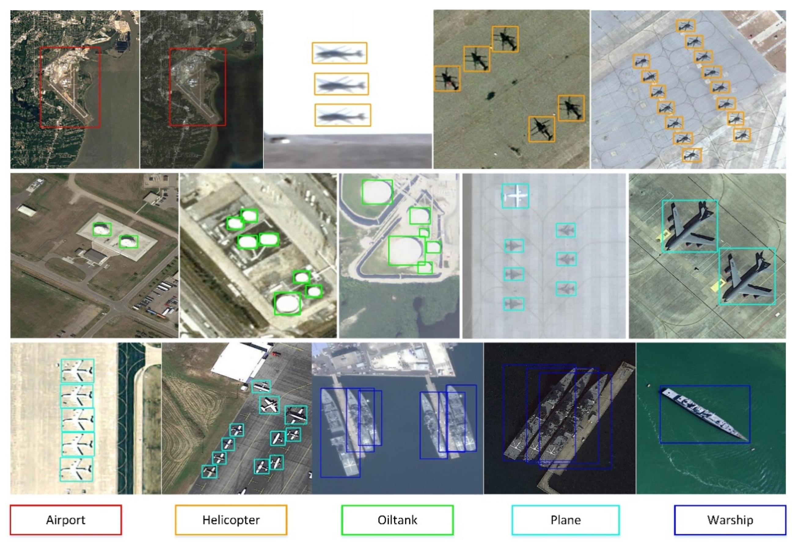
Some examples of images and the corresponding annotated bounding boxes are shown in Figure 1.
It is found that the RSD-GOD has three properties. First, geospatial objects have rich background information, such as different weather conditions, high illumination, low illumination and other background clutters. Second, these remote-sensing images are collected with multiple resolutions and viewpoints, which means multiple scales and angles of the same object. Third, there are some dense objects like planes and warships. It is a great challenge to deal with the complexity of annotated samples for the existing object detection algorithms.
We further analyze the constructed RSD-GOD. According to different sites of remote-sensing images, the dataset is divided into two parts. One is for training, the other is for testing. To adjust hyper-parameters of the proposed model in the training process, 30% of training samples can be randomly selected as a validation dataset. The number of instances in different categories from three sets is shown in Table 1.
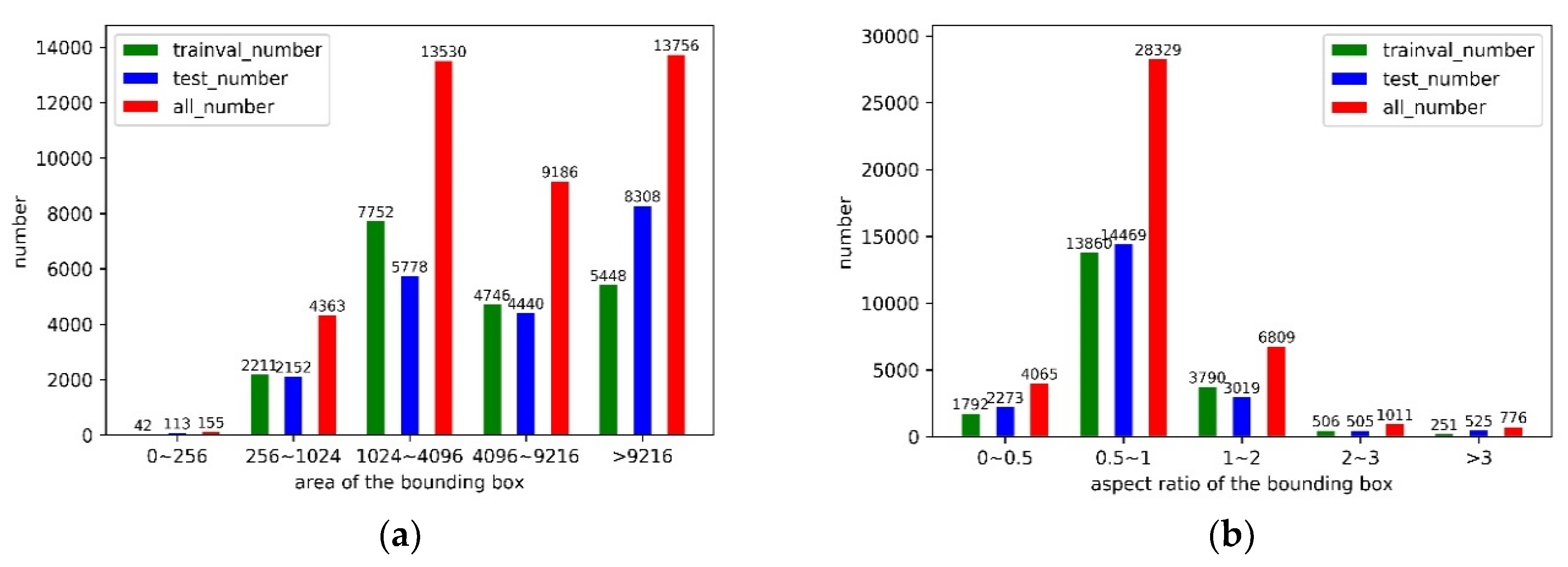
We conduct the statistical analysis of RSD-GOD from two points: area and aspect ratio of the bounding box. The area of the bounding box is divided into five levels: extra-small ( pixels), small ( pixels), middle ( pixels), large ( pixels), and extra-large ( pixels); where is the number of pixels in each bounding box. As shown in Figure 2a, it is found that most of the bounding boxes are in middle and large scales. Specifically, the number of extra-small and small instances is around 4500. The adequate quantity is applicable for training the deep learning-based model and is important in practical detection applications of geospatial objects with small size. The aspect ratio of bounding box is also divided into five levels and over 87% of them are distributed in . These instances with various aspect ratios strengthen the diversity of RSD-GOD. The distribution of aspect ratio is similar to real scenes, which can provide essential information for anchor-based models.
2.2. Single Shot Framework with Multi-Scale Feature Fusion
Our proposed framework is derived from YOLO and SSD that predict bounding boxes and corresponding object categories in a single-shot network. Motivated by the development tendency of computer vision, a deeper base CNN named Darknet-53 is applied to extract features. Considering the challenge of detecting small objects, a multi-scale feature fusion technique is applied. The design of anchors from Faster R-CNN is used to predict object bounding boxes. Furthermore, the k-means clustering method is presented on the training bounding boxes set to obtain anchor priors.
2.2.1. Darknet and Single Shot Framework
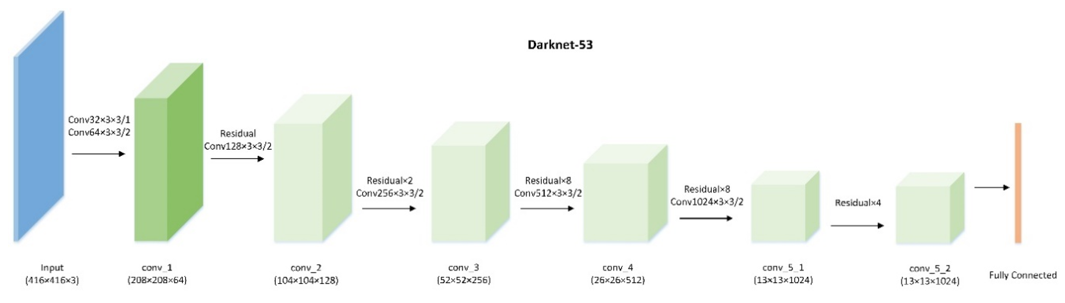
Base feature extractor. A deeper neural network has stronger feature learning and generalization abilities. Generally speaking, the ResNet-101 as a base feature extractor performs better than Visual Geometry Group (VGG) model in the detection framework. In proposed single-shot object detection framework, we construct a superior network to be the feature extractor, as shown in Figure 3, literally named as Darknet-53. Except for the last fully connected layer, there are 53 convolutional layers without any pooling layer. Similar to the VGG-16, filters are mostly used. Instead of max-pooling or average-pooling, the size of the feature map is decreased by a factor of 2 through adjusting the convolutional stride. To make the training of deep network easier, Darknet-53 adopts residual blocks. Each residual block contains and convolutional filters, and 23 residual blocks () are finally used. When optimizing a very deep network, it is important to control overfitting and convergence during the training process. To address this problem, without using the dropout technique, a batch normalization (BN) [50] operation is applied after each convolutional layer in the whole framework. The Leaky ReLU is used as the activation function in each convolutional layer.
Multi-scale feature fusion detector. Most object detection models extract upper features at the top-most layer of a base CNN, including Faster R-CNN [28] and YOLO [30]. Although these methods show powerful detection performance, they do not utilize more local detailed information. The feature maps from different layers contain different object information such as high-level semantic features and low-level fine details. To make full use of the abundant information of the whole feature extractor, multi-scale features are fused to predict bounding boxes. This multi-scale feature fusion detector has inspiring feature representation capacity to cover kinds of geospatial objects with different scales and shapes.
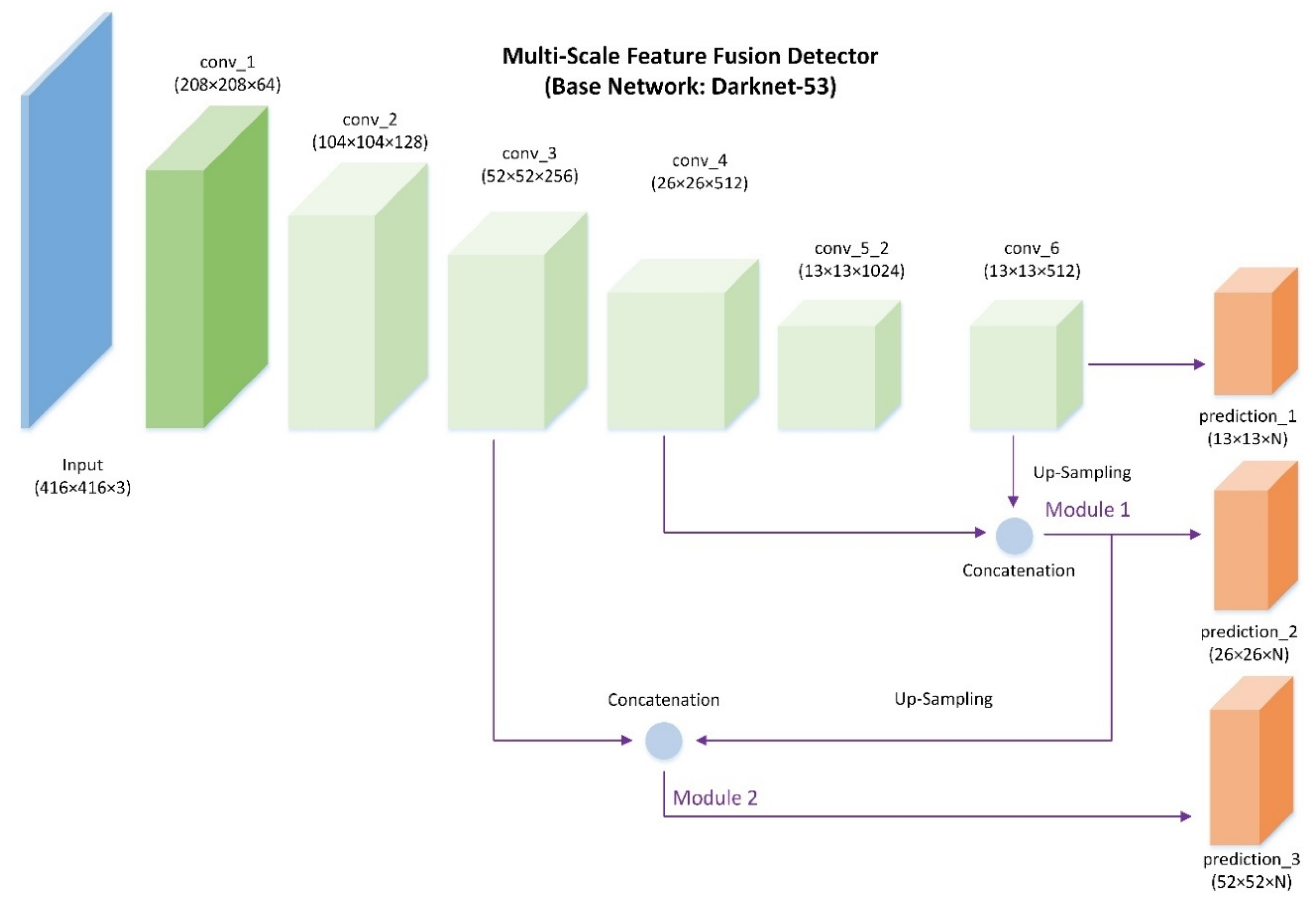
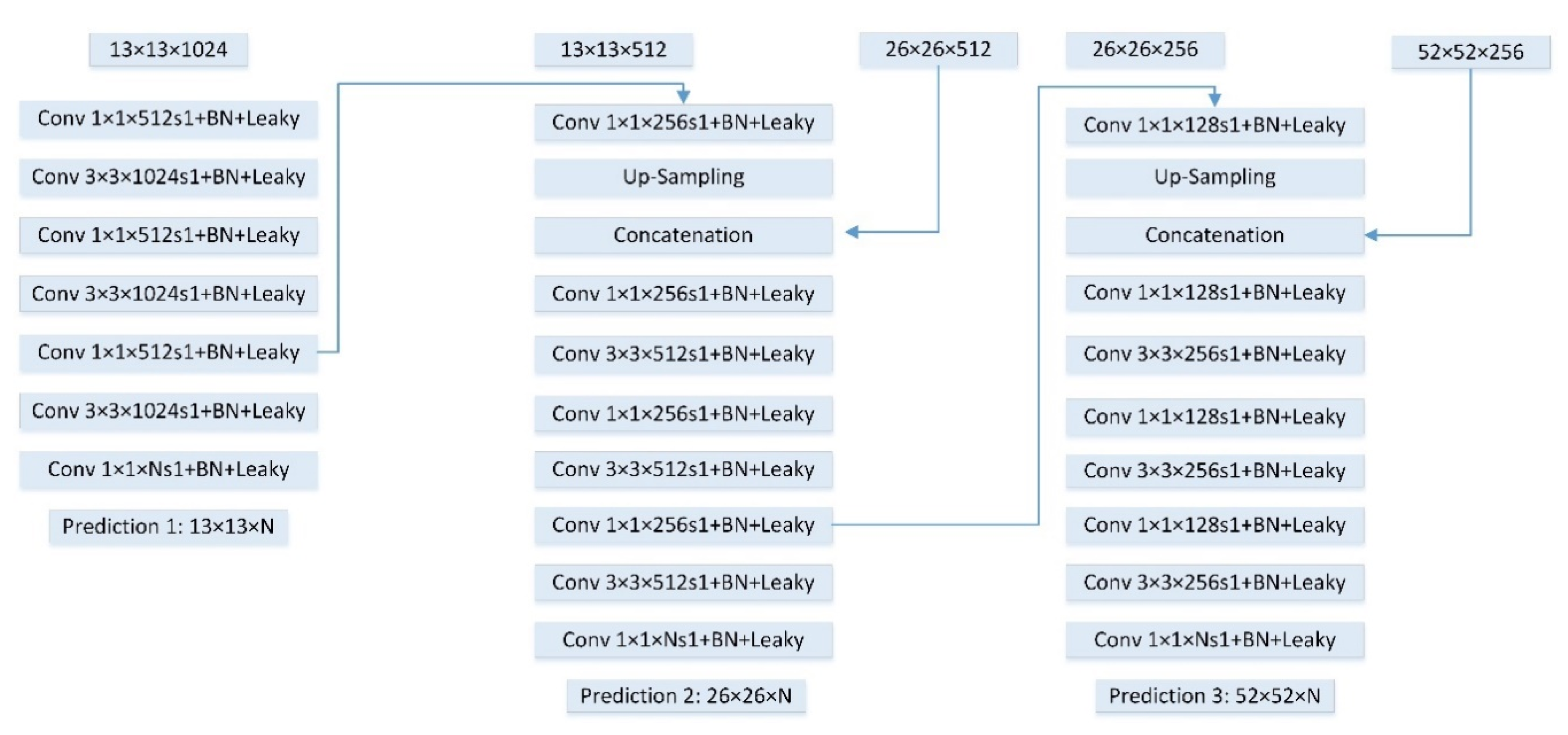
As shown in Figure 4, three convolutional layers at different scales of Darknet-53 are used to make predictions. To make first-scale predictions, we add layer conv_6 after the top-most convolutional layer conv_5_2, which is full of high-level context and semantic information. There are two feature fusion modules to combine shallow features. In feature fusion module 1, conv_6 is up-sampled and then merges with conv_4 through concatenation operation to make second-scale predictions. In feature fusion module 2, the upper fusion module is up-sampled and then merges with conv_3 through the same concatenation method to make third-scale predictions. Different level features are fused to be mainly responsible for detecting small objects (area is smaller than ).
Multi-scale feature fusion module. The specific details of the feature fusion module are described in Figure 5. The dimension of feature maps is reduced firstly with the use of convolutional kernel. High-level feature maps are up-sampled after Conv to be the same size of low-level feature maps. The dimension of low-level features is 2 times higher than high-level features, which means the importance of fine details. Considering the different feature dimension from two scales, concatenation is applied to merge these features. Features extracted from one scale, two scales and three scales are used to generate three predictions. For each scale prediction, the 7 convolutional layers are added using and convolutional kernels. Every pixel in the feature map corresponds to prediction scores that will be explained in the next part.
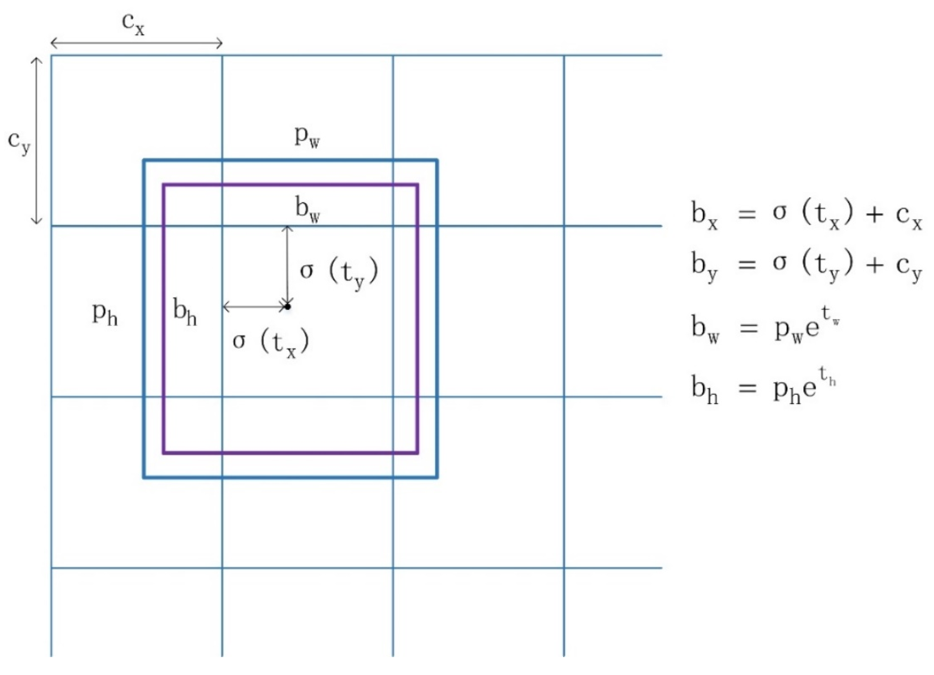
Anchor priors and predictions. The model is unstable especially during early training iterations when the locations of bounding boxes are directly predicted. Motivated by the Faster R-CNN, anchors are introduced and applied to predict bounding boxes in our method. In our designed network, three kinds of feature maps with different size are obtained after convolutional layers down-sampling and multi-scale feature fusion module: , , , which is named as grid (). anchor priors are generated and corresponding bounding boxes are predicted at each grid cell. During the training process, the proposed network outputs 5 coordinate values directly. The final location of the predicted bounding box can be obtained through the anchor priors’ size and the network outputs. As a result, the final prediction and object confidence of bounding boxes at each cell can be calculated as follows.
As shown in Figure 6, the center location of bounding boxes is relative to the grid cell offsets () and the sigmoid activation function value of location coordinates (), where () denotes the offsets from the top left corner of the original image to the current grid cell. The width and height of anchor priors is denoted as (). means the confidence score of object probability. The stands for sigmoid function that limits the values of and to be (0~1). By applying the sigmoid function to normalize the predicted , the model is more stable for training.
At each prediction module, 3 anchor priors with different scales are used which means . The predicted feature maps with different size have different anchor priors. In order to make anchor priors adaptive to a specific dataset, k-means clustering algorithm is applied on the annotated bounding boxes in the training data set to obtain suitable priors. Compared to the hand-picked anchors, the automatic acquired anchor priors based on k-means algorithm make it easier for the network to learn good detections. In our experiments, in each scale prediction module. Due to the three scales, there are finally 9 anchor priors. On our constructed RSD-GOD dataset, the 9 anchor priors are: , , , , , , , , , which corresponds to prediction module 3 (), module 2 () and module 1 (), respectively. The average intersection-over-union (IoU) between anchor priors and ground truth bounding boxes is approximately equal to 0.73.
More than four coordinates and one object confidence information, the grid cell also predicts class probabilities for each bounding box. The dimension of network output tensor is , where ; ; ; in our experiments.
2.2.2. Loss Function
The training objective loss is defined with localization loss (loc), confidence loss (conf) and classification loss (cla). We use squared error loss to compute localization loss and confidence loss. For the multi-class problem, softmax function is applied, and the categorical cross-entropy is computed to obtain classification loss. The overall loss function is defined as:
where , , , and are scaling factors to weight localization loss, confidence loss and classification loss. And denotes the object existing in the anchor box. The predicted bounding box without object is penalized more. In the experiments, we set , , , and .
2.3. Soft Non-Maximum Suppression
Our proposed one-stage detection method generates a large number of cluttered and repetitive bounding boxes in the final three prediction modules. NMS is an integral component of the object detection framework to predict final object detections from a set of location candidates, which effectively improve detection performance. The traditional NMS ranks location candidates according to their classification score. If there is a high overlap between two boxes, bounding box with lower scores will be removed. In our constructed RSD-GOD dataset, there are some dense objects such as warships and small planes. This hard NMS might miss part of neighboring detections whose classification scores are lower. Instead of removing the location candidates directly, the proposed soft-NMS reassign a bounding box a new classification score, which is denoted as follows:
where denotes -th bounding box in the location candidates and is the bounding box with maximum score. If the IoU between and is larger than threshold , a decayed score will be given to with the use of a penalty function:
The reassigned score is associated with the overlap between two boxes. When the IoU is low, these two candidate detections have a high probability to be both true positives. Thus, the should have some effects on the . Specifically, remains unchanged when the overlap is zero. To address this point, the Gaussian penalty function is considered:
3. Results and Discussion
To evaluate the performance of the proposed single-shot object detection approach on remote-sensing images, we compare it with several existing methods. The concise experimental settings are described in this section, including datasets, evaluation metrics, and compared methods. Then, the quantitative and qualitative analysis are brought into the discussion.
3.1. Experimental Settings
3.1.1. Dataset
For reliable evaluation and verification of the proposed method, two datasets are used in our experiments. The first one is RSD-GOD geospatial dataset, which is introduced in Section 2.1 in detail. The RSD-GOD is a challenging 5-class object detection dataset that contains 18,187 images with more than 40,000 instances. We divide the whole RSD-GOD dataset into three parts, 35% for training, 15% for validation, and 50% for testing. Specifically, the location sources of remote-sensing images are different between training validation and testing datasets.
The second one is the NWPU VHR-10 dataset, which contains 10 geospatial object classes. There are two image subsets in NWPU VHR-10 dataset: a positive set including 650 annotated images and a negative set including 150 images without any targets of the given 10 categories. In our experiments, the positive set is divided into 20% for training, 20% for validation and 60% for testing, which corresponds to 130, 130, 390 images respectively.
3.1.2. Evaluation Metrics
To quantitatively evaluate the performance of the proposed framework, the average precision (AP) and precision-recall curve (PRC) are adopted, which are two standard and widely used evaluation metrics in object detection tasks. For better expression, true positives, false positives, and false negatives are denoted as TP, FP and FN. A predicted bounding box is considered to be TP if the IoU between predicted bounding box and ground truth is larger than 0.5. Otherwise, it would be considered as FP. FN denotes that the actual annotated object has no predicted bounding box. Specifically, TP means the correct retrieval of an object. The precision indicator measures the proportion of detections that are TP and the recall indicator measures the fraction of practical annotations that are classified correctly. The calculation formulas of precision and recall are as follows:
During the evaluation process, the recall metric changes from 0 to 1, and precision metric has a corresponding value. Thus, the PRC can be obtained. For each object class, the area under PRC is computed as its AP. The detection method has a better performance when the AP value is higher.
3.1.3. Compared Methods
We compare the proposed network with some typical object detection methods, including two-stage and one-stage detection frameworks.
Faster R-CNN applies a region proposal network to generate object bounds and then classifies these proposed regions using fast R-CNN detector. In our experiments, ResNet-50 is adopted as the base network to extract features. Besides, the pretrained ResNet-50 on a large ImageNet dataset is applied. The learning rate is set to for the first 1000 iterations and then decays to for following 1000 iterations.
SSD predicts object bounding boxes directly using an end-to-end neural network. We choose the VGG-16 to be a feature extractor. Combined with anchor boxes, multiple feature maps from different scales are used to make predictions respectively. The image input size is . The learning rate starts from and then decays by a factor of 0.1 when the training loss does not reduce in five epochs. The batch size is set to be 8. The adopted VGG-16 framework is pretrained on the Pattern Analysis, Statistical Modelling and Computational Learning Visual Object Classes (PASCAL VOC) dataset.
YOLO2 predicts bounding boxes on a feature map. A high-resolution classifier, anchor priors, and multi-scale training techniques are applied to predict location candidates. The darknet-19 is used to extract object features, which has 19 convolutional layers, 5 max-pooling layers and no fully connected layers. For better training, the darknet-19 network has used the pretrained weights on the PASCAL VOC dataset.
The different networks of Faster R-CNN, SSD, YOLO2 and proposed framework are trained in the same training dataset and validated in the same validation dataset. During the training process, data augmentation strategies are all applied in these compared methods, which is described in the following part.
3.1.4. Implementation Details
Data augmentation is performed to automatically increase the number of annotated remote-sensing images, which plays an important role in reducing over-fitting in the training process and improving model generalization ability in the testing stage. In our experiments, random flip horizontally or vertically, crop of the image and random rotation of any angle are adopted. The trained dataset expands the number of original images five-fold. These data augmentation strategies effectively make the detection model more robust to geospatial objects with various scales and shapes, especially for small targets.
In the proposed multi-scale feature fusion detector, the image input size is . Each prediction module has three anchor priors with different scales. Through k-means clustering, the 9 anchor priors are obtained for our RSD-GOD dataset: , , , , , , , , . For the publicly available NWPU VHR-10 dataset, the 9 anchor priors are , , , , , , , , . When the detections are considered to be positive or negative, the IoU threshold is set to be 0.5. The threshold of soft-NMS to determine whether reassign the candidate a decayed score or not is 0.45, and the hyper-parameter in the Gaussian penalty function is 0.5.
During the training procedure, the parameters of base darknet-53 are initialized with the pretrained weights on the large PASCAL VOC dataset. The learning rate starts from and then decays by a factor of 0.1 when the training loss does not reduce in five epochs. An Adam method is adopted for efficient stochastic optimization. Our experiments are implemented with the use of a deep learning library named Keras. The computing environment contains an Intel i7 CPU and NVIDIA GTX-1080Ti GPU with 11 GB memory.
3.2. Results on RSD-GOD Dataset
3.2.1. Quantitative Comparisons
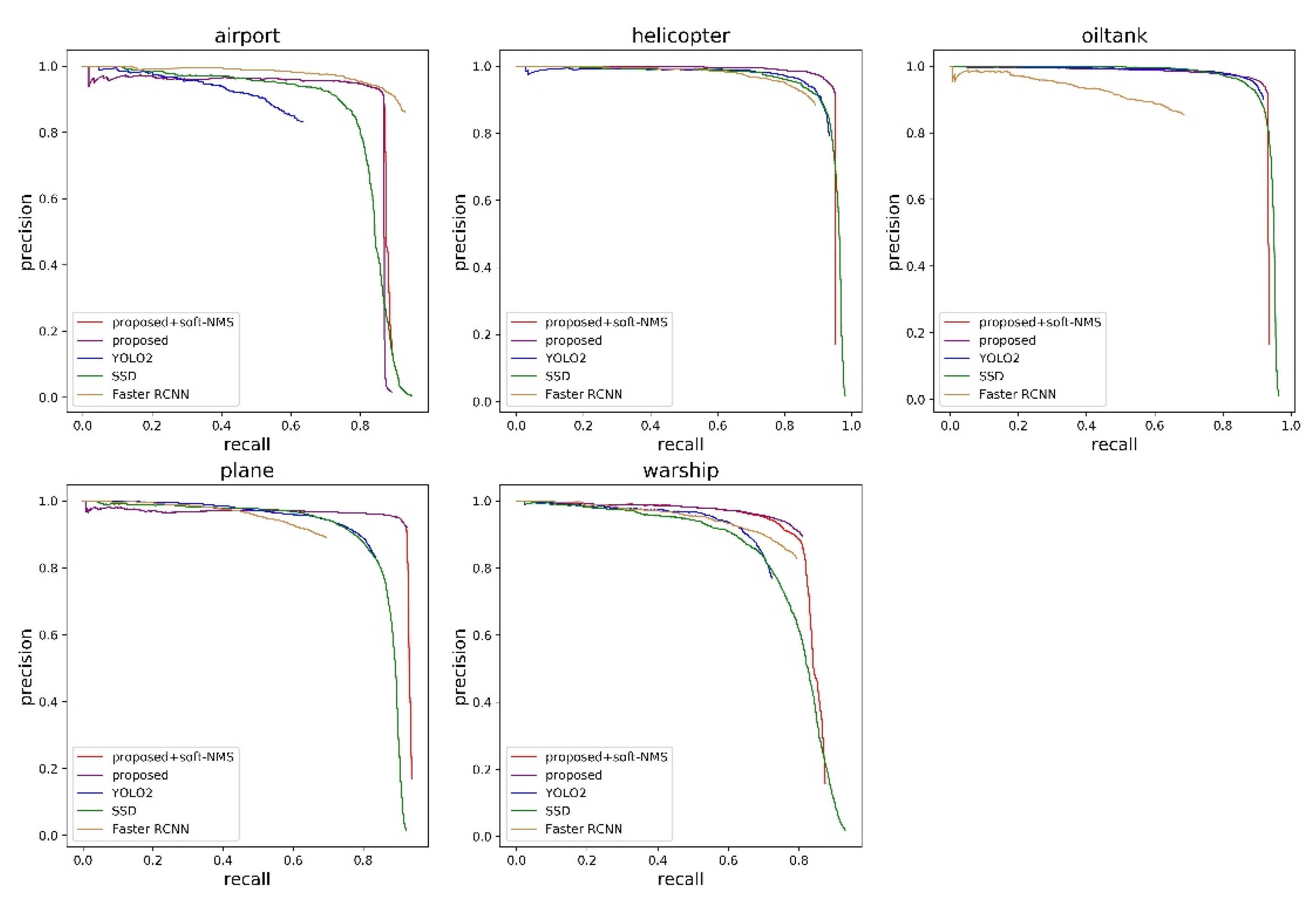
Three different methods as mentioned above are compared to evaluate the performance of our proposed geospatial object detection framework. Quantitative comparison results are shown in Table 2, including AP values of five target categories, and the mean AP of comprehensive assessment. For better visualization and comparison, the PRCs are also displayed in Figure 7. It is found that Faster R-CNN has the highest AP value for airport. However, as shown in Figure 7, it is obvious that Faster R-CNN has lower recalls of oiltank and plane than other methods, which causes the lowest AP value. This may be due to the fact that Faster R-CNN has only selected about 200 regions of interest to be classified in our experiments. Besides, the extracted features from Faster R-CNN have more high-level semantic information that has weak identification ability to detect small objects like the plane. By contrast with the two-stage detection method, the one-stage method predicts a large number of bounding box candidates such as SSD and YOLO2. Compared with YOLO2 that uses the last convolutional layer to make predictions, SSD makes detections at different layers with feature maps of different scales. As a result, it can be seen that SSD obtains a reasonable recall for each class and has a higher mean AP value than YOLO2. As shown in Table 2 and Figure 7, our method achieves the best mean AP value of 87.9%. Apart from the airport, the proposed approach obtains the highest AP values. Compared with the SSD, there are 5.1%, 5.3%, 7.8%, 2.2% and 3.8% performance gains of the proposed network for airport, helicopter, plane, oiltank and warship correspondingly. The proposed method obtains 4.8% performance gains in term of mean AP, which demonstrates the effectiveness of our multi-scale feature fusion detector. It can be inferred that the proposed feature fusion modules play an important role in improving detection performance, especially satisfying detection results for small geospatial targets. With the implementation of soft-NMS, the proposed method achieves a better performance. As can be seen, the soft-NMS algorithm improves the recalls of the warship and plane. The overall mean AP value increases from 87.9% to 89.0%, showing that the soft weighting function can improve the detection performance of neighboring objects.
Considering the object size and ratio analyzed in Section 2.2.1, we further evaluate the proposed method through calculating AP values on various object sizes and ratios. By contrast with the previous five levels of bounding box area, we regard the extra-small and small as one small level (), middle as medium level (), large and extra-large as large level (). The number of instances on the RSD-GOD testing dataset and AP values in different categories from three size levels are shown in Table 3. It can be found that AP value becomes larger with the increasing area of bounding box. Furthermore, the proposed method shows good detection performance on the helicopter and plane with small level size. Similarly, we reallocate the ratio of the bounding box into three levels: wide level (, ), medium level (, ), and tall level (, ). The number of instances on the RSD-GOD testing dataset and AP values in different categories from three ratio levels are shown in Table 4. Compared with the wide or tall level, the medium level of the object ratio mostly achieves the highest AP values. On account of special shape of warship, its ratio mostly distributes in wide and tall level which causes higher AP value of the wide level. We can also infer that a better AP value is obtained when the corresponding number of instances is bigger. This is because more bounding box instances are applied to learn the network parameters in the training process.
3.2.2. Qualitative Analysis
For a better understanding, a number of detection results using the proposed method with soft-NMS are shown in Figure 8. Each target class has four samples that contain various scales, shapes, resolutions and complex backgrounds. The detection results of different kinds of categories are represented with bounding boxes in different colors. Our method shows the effective performance of detecting geospatial objects with remote-sensing images.
As depicted in Figure 8, it is found that the proposed method successfully detects most of the objects. Although the airport has various sizes and shapes, our approach has the ability to extract valid features such as single racetrack or crossed runways and shows robustness to detecting them. Specifically, the airport is covered well with predicted bounding boxes. For closely aligned objects, especially small helicopters, planes and oiltanks, the detection results have a promising and excellent performance. There are only a small number of false alarms. For example, a bounding box candidate containing two planes and backgrounds is regarded as a plane target. In the complex conditions of changing illumination, object shadows, viewpoint variations, blurred targets, varying scales and densely distributed groups, the proposed approach is shown to be effective and sufficient in predicting satisfying object bounding boxes.
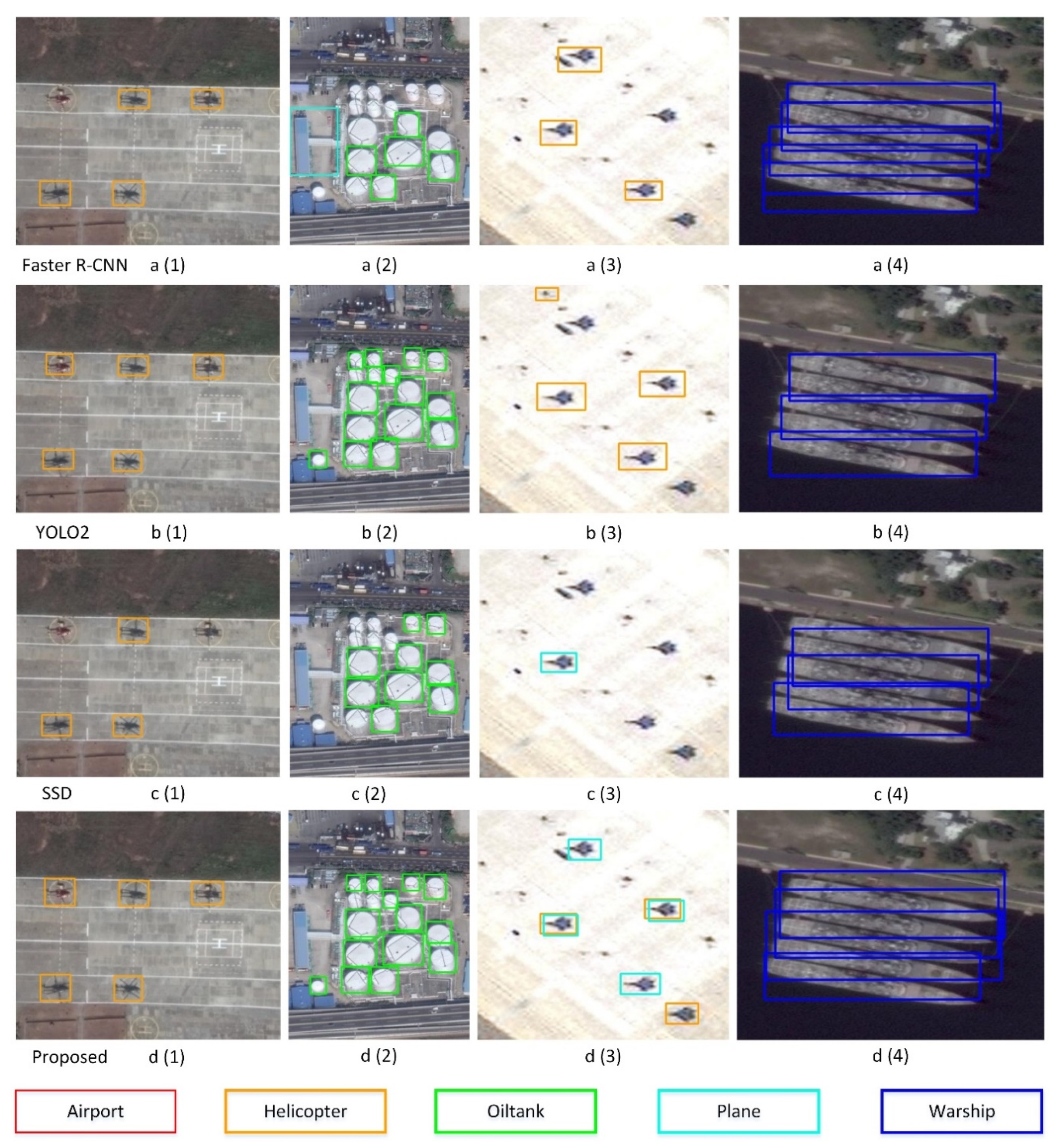
To further demonstrate the detection performance of the proposed network, the qualitative results between our approach and three compared methods are shown in Figure 9. The proposed method performs better than the other three detection frameworks. Compared with YOLO2 and SSD, Faster R-CNN has a good performance in detecting warships of a large scale. SSD and Faster R-CNN have a good deal of missing targets when detecting small objects, such as oiltank and plane. Relatively speaking, the detection results of the helicopter and oiltank demonstrates that our approach has strong ability to predict most of the true bounding boxes except for a few missing objects. Actually, our method will generate some false negatives as shown in Figure 9d (3). This is due to the large number of anchor priors, which cause multiple bounding boxes candidates at neighboring regions. Moreover, it can be found that our approach performs better than comparison methods on detecting warships with the dense distribution.
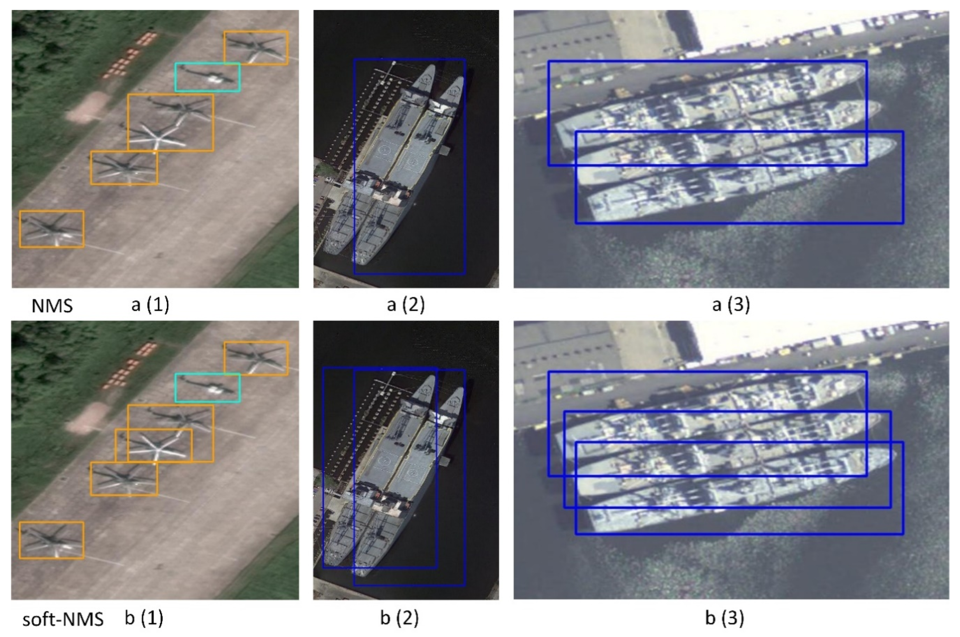
To improve detection performance, our proposed method applies the soft-NMS algorithm. Figure 10 shows the detection results using NMS and soft-NMS. It is obvious that soft-NMS recalls more targets to be detected. When the IoU value between two bounding boxes of different objects is large, the soft-NMS will give one of them a decayed score instead of removing the bounding box. This soft-NMS strategy effectively helps to improve performance on detecting neighboring targets without increasing computational complexity.
3.3. Results on NWPU VHR-10 Dataset
In order to further evaluate the effectiveness and generalization ability of our designed multi-scale feature fusion network, we also train a detector on NWPU VHR-10 dataset. The quantitative results of different methods are shown in Table 5, including AP values of 10 categories and a mean AP measurement. For a more comprehensive evaluation, we add collection of part detectors (COPD) [9], a rotation-invariant CNN (RICNN) [42] model and R-P-Faster R-CNN [5] as comparisons. COPD and RICNN are all rotation-invariant frameworks with an SVM classifier for geospatial object detection. The difference is that COPD uses hand-crafted features while RICNN applies learned features from CNN. It is found that features extracted from the CNN show a better representation ability for detecting objects. Compared with COPD, the mean AP value of RICNN obtains an 18% increase. Faster R-CNN and R-P-Faster R-CNN integrate the region proposal network and classification procedure through sharing the convolutional weights. Compared with RICNN, Faster R-CNN significantly improves AP values for the airplane, baseball diamond, tennis court, basketballcourt and ground track field. Although SSD obtains the highest AP values of the airplane, ship and baseball diamond, it has poor performance in detecting the harbor and bridge. Compared with the traditional and CNN-based methods, the proposed approach has the best performance with a mean AP value of 82.9%. With the application of the soft-NMS algorithm, our network performs better, which achieves nearly 1% performance gains in terms of mean AP. It can be found that our method obtains the best detection results on the storage tank, tennis court, harbor, bridge and vehicle, showing that the proposed multi-scale feature fusion network is effective and robust to detect objects with a small size, a high aspect ratio or variable shapes.
3.4. Efficiency Analysis of Proposed Model
To verify the efficiency of our approach, the running time of different methods is evaluated. Table 6 shows the average running time when one image is tested. RICNN has the lowest computational efficiency due to its multiple detection stages. Compared with the two-stage detection framework such as Faster R-CNN and R-P-Faster R-CNN, the single-shot network has a fast inference speed. It is found that SSD and YOLO2 have less computing time than our method. However, considering the tradeoff between speed and detection performance, the proposed approach achieves effective detections with a fast running time of 0.057 s. With the help of a suitable GPU, our proposed multi-scale feature fusion framework can achieve the inspiring detection results with high computation efficiency, which is able to detect geospatial objects in real-time.
4. Conclusions
In this paper, we firstly construct a novel remote-sensing dataset named RSD-GOD, especially for martial object detection. Secondly, a single-shot geospatial object detection framework based on multi-scale feature fusion modules has been proposed. Feature maps from different layers are merged through up-sampling and concatenation operations, which finally generates pyramid feature maps. These fused features predict bounding box candidates at three scales. The proposed detector with the use of multi-scale feature fusion modules achieves an effective performance. We can draw the conclusions through the experimental results on RSD-GOD and NWPU VHR-10 datasets: (1) The proposed method demonstrates the effectiveness and the better detection performance compared with existing approaches. Specifically, our single-shot detection network achieves a good tradeoff between superior detection accuracy and computation efficiency. (2) The multi-scale feature fusion modules make full use of sufficient local details and high-level semantic information, which shows strong feature representation ability to detect small objects. (3) The soft-NMS algorithm improves the detection performance when there are densely distributed targets. In future work, we will focus on generating more accurate anchor box candidates, and design more powerful matching strategies in the training process.
Author Contributions
S.Z. and P.W. proposed the method for this work, conducted the experiments and drafted the manuscript. B.J., C.W. and G.W. contributed in constructing the dataset, designing the experiments and providing technical supports. All authors read and approved the final manuscript.
Funding
This work was funded by CETC Key Laboratory of Aerospace Information Applications (Grant No. XX17629X009).
Acknowledgments
The authors thank students in the laboratory who have made great contributions to labeling the original remote-sensing images.
Conflicts of Interest
The authors declare no conflict of interest.
References
- Chen, Z.; Zhang, T.; Ouyang, C. End-to-End Airplane Detection Using Transfer Learning in Remote Sensing Images. Remote Sens. 2018, 10, 139. [Google Scholar] [CrossRef]
- Kembhavi, A.; Harwood, D.; Davis, L.S. Vehicle Detection Using Partial Least Squares. IEEE Trans. Pattern Anal. Mach. Intell. 2011, 33, 1250–1265. [Google Scholar] [CrossRef]
- Tuermer, S.; Kurz, F.; Reinartz, P.; Stilla, U. Airborne Vehicle Detection in Dense Urban Areas Using HoG Features and Disparity Maps. IEEE J. Sel. Top. Appl. Earth Obs. Remote Sens. 2013, 6, 2327–2337. [Google Scholar] [CrossRef]
- Grabner, H.; Nguyen, T.T.; Gruber, B.; Bischof, H. On-line boosting-based car detection from aerial images. ISPRS J. Photogramm. Remote Sens. 2008, 63, 382–396. [Google Scholar] [CrossRef]
- Han, X.; Zhong, Y.; Zhang, L. An Efficient and Robust Integrated Geospatial Object Detection Framework for High Spatial Resolution Remote Sensing Imagery. Remote Sens. 2017, 9, 666. [Google Scholar] [CrossRef]
- Zhang, F.; Du, B.; Zhang, L.; Xu, M. Weakly Supervised Learning Based on Coupled Convolutional Neural Networks for Aircraft Detection. IEEE Trans. Geosci. Remote Sens. 2016, 54, 5553–5563. [Google Scholar] [CrossRef]
- Liu, K.; Mattyus, G. Fast Multiclass Vehicle Detection on Aerial Images. IEEE Geosci. Remote Sens. Lett. 2015, 12, 1938–1942. [Google Scholar]
- Liu, Z.; Wang, H.; Weng, L.; Yang, Y. Ship Rotated Bounding Box Space for Ship Extraction from High-Resolution Optical Satellite Images With Complex Backgrounds. IEEE Geosci. Remote Sens. Lett. 2016, 13, 1074–1078. [Google Scholar] [CrossRef]
- Cheng, G.; Han, J.; Zhou, P.; Guo, L. Multi-class geospatial object detection and geographic image classification based on collection of part detectors. ISPRS J. Photogramm. Remote Sens. 2014, 98, 119–132. [Google Scholar] [CrossRef]
- Cheng, G.; Han, J. A survey on object detection in optical remote sensing images. ISPRS J. Photogramm. Remote Sens. 2016, 117, 11–28. [Google Scholar] [CrossRef]
- Ojala, T.; Pietikainen, M.; Maenpaa, T. Multiresolution gray-scale and rotation invariant texture classification with local binary patterns. IEEE Trans. Pattern Anal. Mach. Intell. 2002, 24, 971–987. [Google Scholar] [CrossRef]
- Dalal, N.; Triggs, B. Histograms of Oriented Gradients for Human Detection. In Proceedings of the 2005 IEEE Computer Society Conference on Computer Vision and Pattern Recognition (CVPR’05), San Diego, CA, USA, 20–25 June 2005; IEEE: San Diego, CA, USA, 2005; Volume 1, pp. 886–893. [Google Scholar]
- Li, F.; Perona, P. A Bayesian Hierarchical Model for Learning Natural Scene Categories. In Proceedings of the 2005 IEEE Computer Society Conference on Computer Vision and Pattern Recognition (CVPR’05), San Diego, CA, USA, 20–25 June 2005; IEEE: San Diego, CA, USA, 2005; Volume 2, pp. 524–531. [Google Scholar]
- Tao, C.; Tan, Y.; Cai, H.; Tian, J. Airport Detection From Large IKONOS Images Using Clustered SIFT Keypoints and Region Information. IEEE Geosci. Remote Sens. Lett. 2011, 8, 128–132. [Google Scholar] [CrossRef]
- Aytekin, Ö.; Zongur, U.; Halici, U. Texture-Based Airport Runway Detection. IEEE Geosci. Remote Sens. Lett. 2013, 10, 471–475. [Google Scholar] [CrossRef]
- Zhang, D.; Han, J.; Cheng, G.; Liu, Z.; Bu, S.; Guo, L. Weakly Supervised Learning for Target Detection in Remote Sensing Images. IEEE Geosci. Remote Sens. Lett. 2015, 12, 701–705. [Google Scholar] [CrossRef]
- Han, J.; Zhang, D.; Cheng, G.; Guo, L.; Ren, J. Object Detection in Optical Remote Sensing Images Based on Weakly Supervised Learning and High-Level Feature Learning. IEEE Trans. Geosci. Remote Sens. 2015, 53, 3325–3337. [Google Scholar] [CrossRef]
- Cheng, G.; Han, J.; Guo, L.; Qian, X.; Zhou, P.; Yao, X.; Hu, X. Object detection in remote sensing imagery using a discriminatively trained mixture model. ISPRS J. Photogramm. Remote Sens. 2013, 85, 32–43. [Google Scholar] [CrossRef]
- Sun, H.; Sun, X.; Wang, H.; Li, Y.; Li, X. Automatic Target Detection in High-Resolution Remote Sensing Images Using Spatial Sparse Coding Bag-of-Words Model. IEEE Geosci. Remote Sens. Lett. 2012, 9, 109–113. [Google Scholar] [CrossRef]
- Zhang, W.; Sun, X.; Fu, K.; Wang, C.; Wang, H. Object Detection in High-Resolution Remote Sensing Images Using Rotation Invariant Parts Based Model. IEEE Geosci. Remote Sens. Lett. 2014, 11, 74–78. [Google Scholar] [CrossRef]
- Mountrakis, G.; Im, J.; Ogole, C. Support vector machines in remote sensing: A review. ISPRS J. Photogramm. Remote Sens. 2011, 66, 247–259. [Google Scholar] [CrossRef]
- Bi, F.; Zhu, B.; Gao, L.; Bian, M. A Visual Search Inspired Computational Model for Ship Detection in Optical Satellite Images. IEEE Geosci. Remote Sens. Lett. 2012, 9, 749–753. [Google Scholar]
- Leitloff, J.; Hinz, S.; Stilla, U. Vehicle Detection in Very High Resolution Satellite Images of City Areas. IEEE Trans. Geosci. Remote Sens. 2010, 48, 2795–2806. [Google Scholar] [CrossRef]
- Shi, Z.; Yu, X.; Jiang, Z.; Li, B. Ship Detection in High-Resolution Optical Imagery Based on Anomaly Detector and Local Shape Feature. IEEE Trans. Geosci. Remote Sens. 2014, 52, 4511–4523. [Google Scholar]
- Girshick, R.; Donahue, J.; Darrell, T.; Malik, J. Rich feature hierarchies for accurate object detection and semantic segmentation. arXiv, 2013; arXiv:1311.2524. [Google Scholar]
- Girshick, R. Fast R-CNN. In Proceedings of the 2015 IEEE International Conference on Computer Vision (ICCV), Santiago, Chile, 13–16 December 2015; IEEE: Santiago, Chile, 2015; pp. 1440–1448. [Google Scholar]
- Uijlings, J.R.R.; van de Sande, K.E.A.; Gevers, T.; Smeulders, A.W.M. Selective Search for Object Recognition. Int. J. Comput. Vis. 2013, 104, 154–171. [Google Scholar] [CrossRef]
- Ren, S.; He, K.; Girshick, R.; Sun, J. Faster R-CNN: Towards Real-Time Object Detection with Region Proposal Networks. IEEE Trans. Pattern Anal. Mach. Intell. 2017, 39, 1137–1149. [Google Scholar] [CrossRef]
- Redmon, J.; Divvala, S.; Girshick, R.; Farhadi, A. You Only Look Once: Unified, Real-Time Object Detection. arXiv, 2015; arXiv:1506.02640. [Google Scholar]
- Redmon, J.; Farhadi, A. YOLO9000: Better, Faster, Stronger. arXiv, 2016; arXiv:1612.08242. [Google Scholar]
- Liu, W.; Anguelov, D.; Erhan, D.; Szegedy, C.; Reed, S.; Fu, C.-Y.; Berg, A.C. SSD: Single Shot MultiBox Detector. In Computer Vision—ECCV 2016; Leibe, B., Matas, J., Sebe, N., Welling, M., Eds.; Springer International Publishing: Cham, Switzerland, 2016; Volume 9905, pp. 21–37. ISBN 978-3-319-46447-3. [Google Scholar]
- Dai, J.; Li, Y.; He, K.; Sun, J. R-FCN: Object Detection via Region-based Fully Convolutional Networks. arXiv, 2016; arXiv:1605.06409. [Google Scholar]
- Xu, M.; Cui, L.; Lv, P.; Jiang, X.; Niu, J.; Zhou, B.; Wang, M. MDSSD: Multi-scale Deconvolutional Single Shot Detector for Small Objects. arXiv, 2018; arXiv:1805.07009. [Google Scholar]
- Fu, C.-Y.; Liu, W.; Ranga, A.; Tyagi, A.; Berg, A.C. DSSD: Deconvolutional Single Shot Detector. arXiv, 2017; arXiv:1701.06659. [Google Scholar]
- Redmon, J.; Farhadi, A. YOLOv3: An Incremental Improvement. arXiv, 2018; arXiv:1804.02767. [Google Scholar]
- Xie, H.; Wang, T.; Qiao, M.; Zhang, M.; Shan, G.; Snoussi, H. Robust object detection for tiny and dense targets in VHR aerial images. In Proceedings of the 2017 Chinese Automation Congress (CAC), Jinan, China, 20–22 October 2017; IEEE: Jinan, China, 2017; pp. 6397–6401. [Google Scholar]
- Long, Y.; Gong, Y.; Xiao, Z.; Liu, Q. Accurate Object Localization in Remote Sensing Images Based on Convolutional Neural Networks. IEEE Trans. Geosci. Remote Sens. 2017, 55, 2486–2498. [Google Scholar] [CrossRef]
- Zhong, Y.; Han, X.; Zhang, L. Multi-class geospatial object detection based on a position-sensitive balancing framework for high spatial resolution remote sensing imagery. ISPRS J. Photogramm. Remote Sens. 2018, 138, 281–294. [Google Scholar] [CrossRef]
- Zou, Z.; Shi, Z. Ship Detection in Spaceborne Optical Image With SVD Networks. IEEE Trans. Geosci. Remote Sens. 2016, 54, 5832–5845. [Google Scholar] [CrossRef]
- Yang, X.; Sun, H.; Fu, K.; Yang, J.; Sun, X.; Yan, M.; Guo, Z. Automatic Ship Detection in Remote Sensing Images from Google Earth of Complex Scenes Based on Multiscale Rotation Dense Feature Pyramid Networks. Remote Sens. 2018, 10, 132. [Google Scholar] [CrossRef]
- Miao, K.; Ji, K.; Leng, X.; Lin, Z. Contextual Region-Based Convolutional Neural Network with Multilayer Fusion for SAR Ship Detection. Remote Sens. 2017, 9, 860. [Google Scholar] [CrossRef]
- Cheng, G.; Zhou, P.; Han, J. Learning Rotation-Invariant Convolutional Neural Networks for Object Detection in VHR Optical Remote Sensing Images. IEEE Trans. Geosci. Remote Sens. 2016, 54, 7405–7415. [Google Scholar] [CrossRef]
- Cai, B.; Jiang, Z.; Zhang, H.; Zhao, D.; Yao, Y. Airport Detection Using End-to-End Convolutional Neural Network with Hard Example Mining. Remote Sens. 2017, 9, 1198. [Google Scholar] [CrossRef]
- Xu, Y.; Zhu, M.; Li, S.; Feng, H.; Ma, S.; Che, J. End-to-End Airport Detection in Remote Sensing Images Combining Cascade Region Proposal Networks and Multi-Threshold Detection Networks. Remote Sens. 2018, 10, 1516. [Google Scholar] [CrossRef]
- Guo, W.; Yang, W.; Zhang, H.; Hua, G. Geospatial Object Detection in High Resolution Satellite Images Based on Multi-Scale Convolutional Neural Network. Remote Sens. 2018, 10, 131. [Google Scholar] [CrossRef]
- Deng, Z.; Sun, H.; Zhou, S.; Zhao, J.; Lei, L.; Zou, H. Multi-scale object detection in remote sensing imagery with convolutional neural networks. ISPRS J. Photogramm. Remote Sens. 2018, 145, 3–22. [Google Scholar] [CrossRef]
- Ren, Y.; Zhu, C.; Xiao, S. Deformable Faster R-CNN with Aggregating Multi-Layer Features for Partially Occluded Object Detection in Optical Remote Sensing Images. Remote Sens. 2018, 10, 1470. [Google Scholar] [CrossRef]
- Li, Z.; Zhou, F. FSSD: Feature Fusion Single Shot Multibox Detector. arXiv, 2017; arXiv:1712.00960. [Google Scholar]
- Bodla, N.; Singh, B.; Chellappa, R.; Davis, L.S. Soft-NMS—Improving Object Detection with One Line of Code. arXiv, 2017; arXiv:1704.04503. [Google Scholar]
- Ioffe, S.; Szegedy, C. Batch Normalization: Accelerating Deep Network Training by Reducing Internal Covariate Shift. arXiv, 2015; arXiv:1502.03167v3. [Google Scholar]
Sample Availability: Computer code of the proposed method and the constructed RSD-GOD dataset is available at: https://github.com/ZhuangShuoH/geospatial-object-detection. |
Figure 1.
Example images and annotated bounding boxes of the remote-sensing dataset for geospatial object detection (RSD-GOD). There are 5 classical geospatial categories, including airport, helicopter, oiltank, plane, and warship. Different object categories are indicated by different color rectangles.

Figure 2.
Statistical information of the constructed RSD-GOD. Statistical results of the training-validation, testing and the entire dataset are depicted as bars with different colors. (a) Number of instances with different area of the bounding box in different datasets; (b) number of instances with different aspect ratio of the bounding box in different datasets.

Figure 3.
Darknet-53: the base network to extract features in the single-shot object detection framework.
Figure 3.
Darknet-53: the base network to extract features in the single-shot object detection framework.

Figure 4.
Multi-scale feature fusion detector. Darknet-53 is the base feature extractor. Three predictions are generated at three different scales.
Figure 4.
Multi-scale feature fusion detector. Darknet-53 is the base feature extractor. Three predictions are generated at three different scales.

Figure 5.
Multi-scale feature fusion module. Feature maps from different layers are merged through up-sampling and concatenation operations, which then predict object detections. Each convolutional layer is followed with a batch normalization (BN) layer and a Leaky ReLU layer. The stride of convolution is 1 (s1).

Figure 6.
Anchor priors and location prediction. The framework directly generates 4 coordinates . The center location of final bounding boxes is relative to the grid cell offsets () and the sigmoid activation function value of location coordinates (), where () denotes the offsets from the top left corner of the original image to the current grid cell. The width and height of anchor priors is denoted as (). The stands for sigmoid function that limits the values of and to be (0~1).

Figure 7.
The precision recall curve of proposed approach and other comparison methods.

Figure 8.
Example images and detection results on RSD-GOD dataset using the proposed approach.

Figure 9.
Detection results on the RSD-GOD dataset with the proposed approach and the other three comparison methods.
Figure 9.
Detection results on the RSD-GOD dataset with the proposed approach and the other three comparison methods.

Figure 10.
Detection results on the constructed RSD-GOD dataset when using non-maximum suppression (NMS) or soft-NMS in the proposed network.
Figure 10.
Detection results on the constructed RSD-GOD dataset when using non-maximum suppression (NMS) or soft-NMS in the proposed network.


Table 1.
The number of instances in three sets.
| Category | Number of Instances | ||
|---|---|---|---|
| Training Set | Validation Set | Testing Set | |
| airport | 1151 | 525 | 1721 |
| helicopter | 2460 | 1763 | 2208 |
| oiltank | 2969 | 2093 | 5113 |
| plane | 3216 | 3034 | 7884 |
| warship | 2123 | 865 | 3865 |
| total | 11,919 | 8280 | 20,791 |
Table 2.
The average precision (AP) values of compared object detection methods on RSD-GOD dataset.
| Method | Faster R-CNN | SSD | YOLO2 | Proposed | Proposed (Soft NMS) |
|---|---|---|---|---|---|
| Pretrained backbone | ResNet50 | VGG16 | Darknet-19 | Darknet-53 | Darknet-53 |
| Airport | 0.911 | 0.788 | 0.598 | 0.839 | 0.847 |
| Helicopter | 0.876 | 0.893 | 0.917 | 0.946 | 0.946 |
| Plane | 0.673 | 0.819 | 0.813 | 0.897 | 0.904 |
| Oiltank | 0.645 | 0.898 | 0.909 | 0.920 | 0.922 |
| Warship | 0.759 | 0.755 | 0.695 | 0.793 | 0.826 |
| Mean AP | 0.773 | 0.831 | 0.786 | 0.879 | 0.890 |
Table 3.
The AP values of different object sizes on RSD-GOD testing dataset.
| Category | Number of Instances | AP Values | ||||
|---|---|---|---|---|---|---|
| Airport | 0 | 20 | 1701 | - | 0.400 | 0.895 |
| Helicopter | 121 | 819 | 1268 | 0.810 | 0.934 | 0.979 |
| Plane | 1461 | 2885 | 3538 | 0.849 | 0.959 | 0.957 |
| Oiltank | 669 | 1631 | 2813 | 0.683 | 0.946 | 0.989 |
| Warship | 21 | 429 | 3415 | - | 0.676 | 0.906 |
Table 4.
The AP values of different object ratios on RSD-GOD testing dataset.
| Category | Number of Instances | AP Values | ||||
|---|---|---|---|---|---|---|
| Airport | 378 | 738 | 605 | 0.828 | 0.949 | 0.856 |
| Helicopter | 66 | 1835 | 307 | 0.758 | 0.967 | 0.915 |
| Plane | 299 | 6760 | 825 | 0.873 | 0.947 | 0.887 |
| Oiltank | 11 | 4811 | 291 | 0.818 | 0.942 | 0.838 |
| Warship | 1565 | 739 | 1561 | 0.919 | 0.847 | 0.845 |
Table 5.
The AP values of compared object detection methods on NWPU VHR-10 dataset.
| Method | COPD | R-P-Faster R-CNN | RICNN | SSD | Faster R-CNN | YOLO2 | Proposed | Proposed (Soft-NMS) |
|---|---|---|---|---|---|---|---|---|
| Airplane | 0.623 | 0.904 | 0.884 | 0.957 | 0.946 | 0.733 | 0.929 | 0.934 |
| Ship | 0.689 | 0.750 | 0.773 | 0.829 | 0.823 | 0.749 | 0.765 | 0.771 |
| Storage tank | 0.637 | 0.444 | 0.853 | 0.856 | 0.653 | 0.344 | 0.849 | 0.875 |
| Baseball diamond | 0.833 | 0.899 | 0.881 | 0.966 | 0.955 | 0.889 | 0.930 | 0.930 |
| Tennis court | 0.321 | 0.797 | 0.408 | 0.821 | 0.819 | 0.291 | 0.824 | 0.827 |
| Basketball court | 0.363 | 0.776 | 0.585 | 0.860 | 0.897 | 0.276 | 0.815 | 0.838 |
| Ground track field | 0.853 | 0.877 | 0.867 | 0.582 | 0.924 | 0.988 | 0.837 | 0.837 |
| Harbor | 0.553 | 0.791 | 0.686 | 0.548 | 0.724 | 0.754 | 0.816 | 0.825 |
| Bridge | 0.148 | 0.682 | 0.615 | 0.419 | 0.575 | 0.518 | 0.702 | 0.725 |
| Vehicle | 0.440 | 0.732 | 0.711 | 0.756 | 0.778 | 0.513 | 0.819 | 0.823 |
| Mean AP | 0.546 | 0.765 | 0.726 | 0.759 | 0.809 | 0.605 | 0.829 | 0.838 |
Table 6.
The average testing time of compared object detection methods.
| Methods | COPD | R-P-Faster R-CNN | RICNN | SSD | Faster R-CNN | YOLO2 | Proposed |
|---|---|---|---|---|---|---|---|
| Backbone | - | VGG16 | - | VGG16 | ResNet50 | Darknet-19 | Darknet-53 |
| Average running time (s) | 1.070 | 0.150 | 8.770 | 0.027 | 0.430 | 0.026 | 0.057 |
© 2019 by the authors. Licensee MDPI, Basel, Switzerland. This article is an open access article distributed under the terms and conditions of the Creative Commons Attribution (CC BY) license (http://creativecommons.org/licenses/by/4.0/).
Share and Cite
MDPI and ACS Style
Zhuang, S.; Wang, P.; Jiang, B.; Wang, G.; Wang, C. A Single Shot Framework with Multi-Scale Feature Fusion for Geospatial Object Detection. Remote Sens. 2019, 11, 594. https://0-doi-org.brum.beds.ac.uk/10.3390/rs11050594
AMA Style
Zhuang S, Wang P, Jiang B, Wang G, Wang C. A Single Shot Framework with Multi-Scale Feature Fusion for Geospatial Object Detection. Remote Sensing. 2019; 11(5):594. https://0-doi-org.brum.beds.ac.uk/10.3390/rs11050594
Chicago/Turabian StyleZhuang, Shuo, Ping Wang, Boran Jiang, Gang Wang, and Cong Wang. 2019. "A Single Shot Framework with Multi-Scale Feature Fusion for Geospatial Object Detection" Remote Sensing 11, no. 5: 594. https://0-doi-org.brum.beds.ac.uk/10.3390/rs11050594
Note that from the first issue of 2016, this journal uses article numbers instead of page numbers. See further details here.