Long-Term Land Cover Dynamics (1986–2016) of Northeast China Derived from a Multi-Temporal Landsat Archive

 , , and
Abstract
:1. Introduction
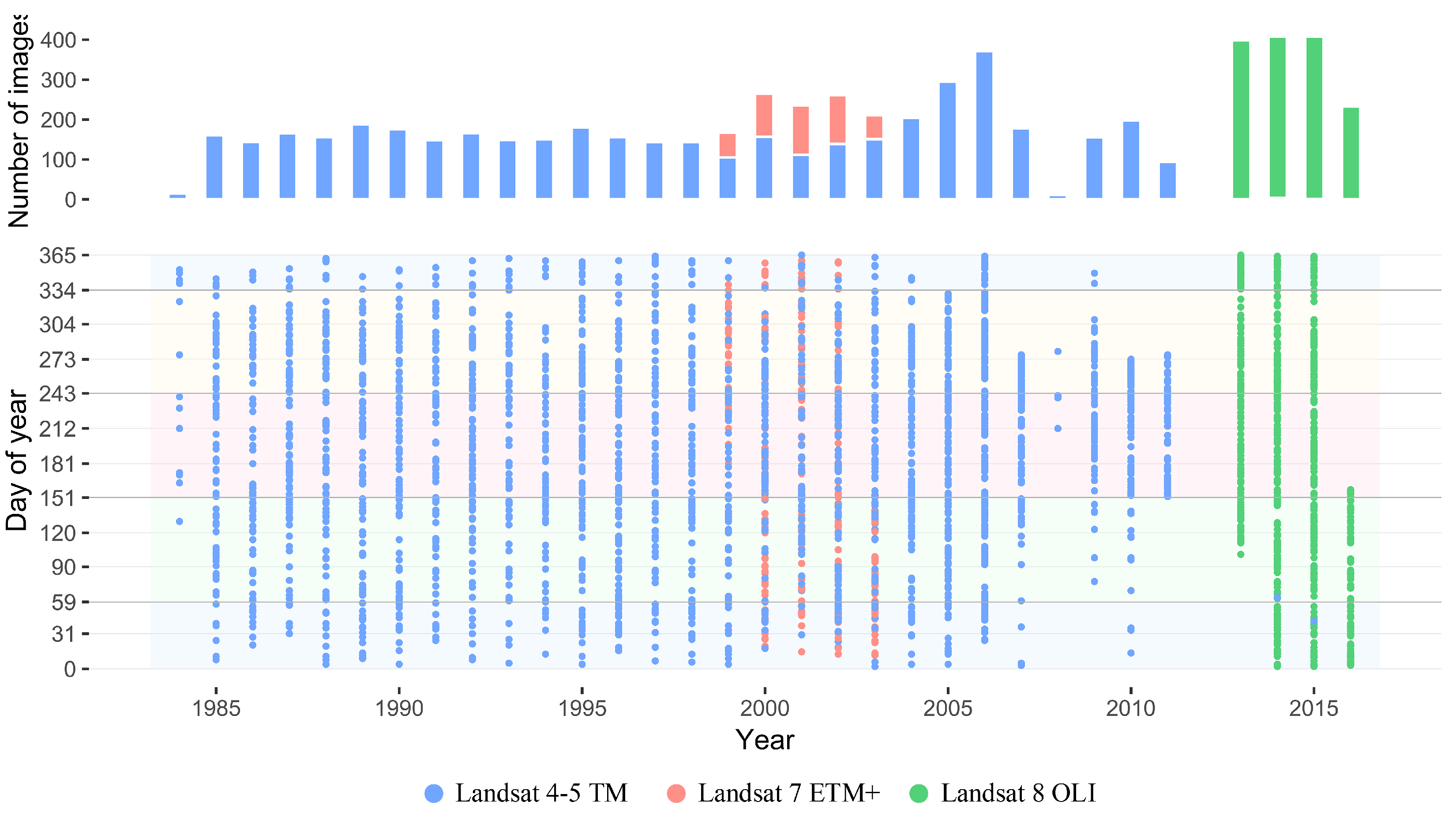
2. Data
3. Methods
3.1. Training Sample Collection
3.2. Classification
3.3. Post-Classification Processing
3.3.1. Seasonal Integration
3.3.2. Temporal Consistency Correction
3.4. Accuracy Assessment
4. Results
4.1. Accuracy of the Maps
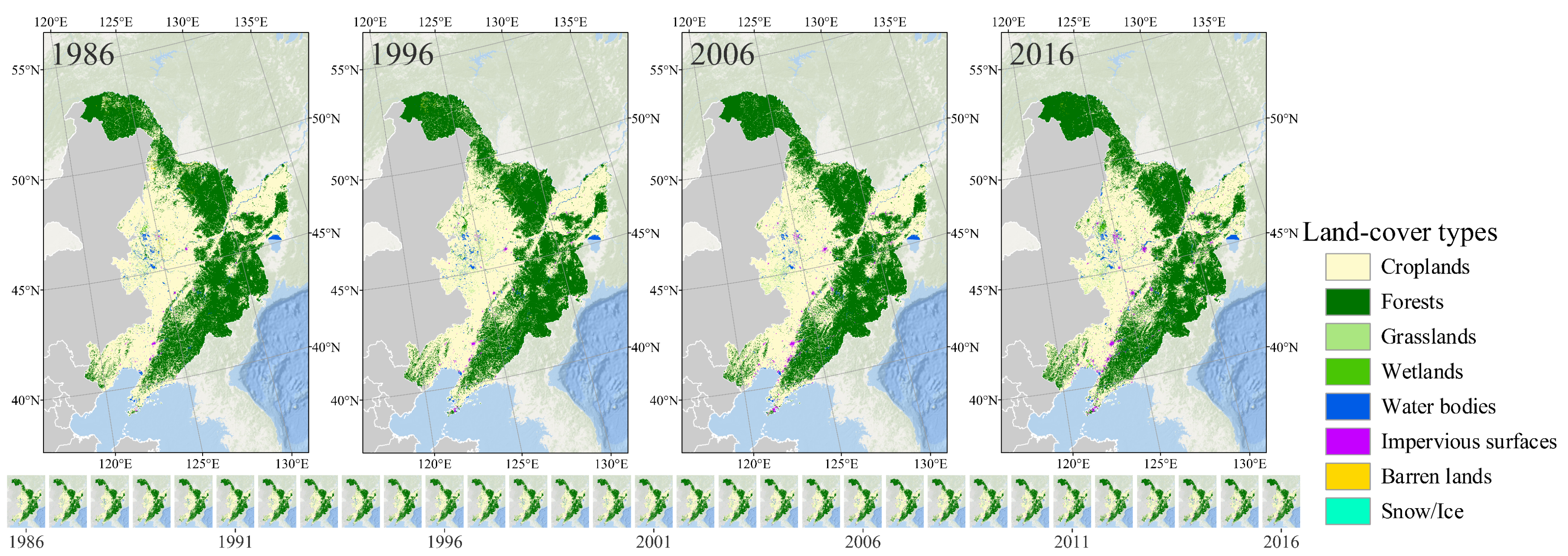
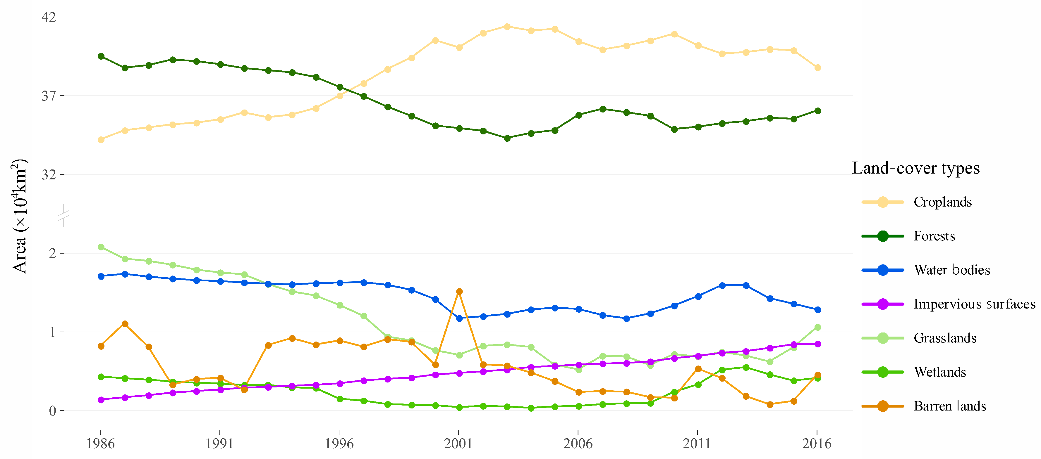
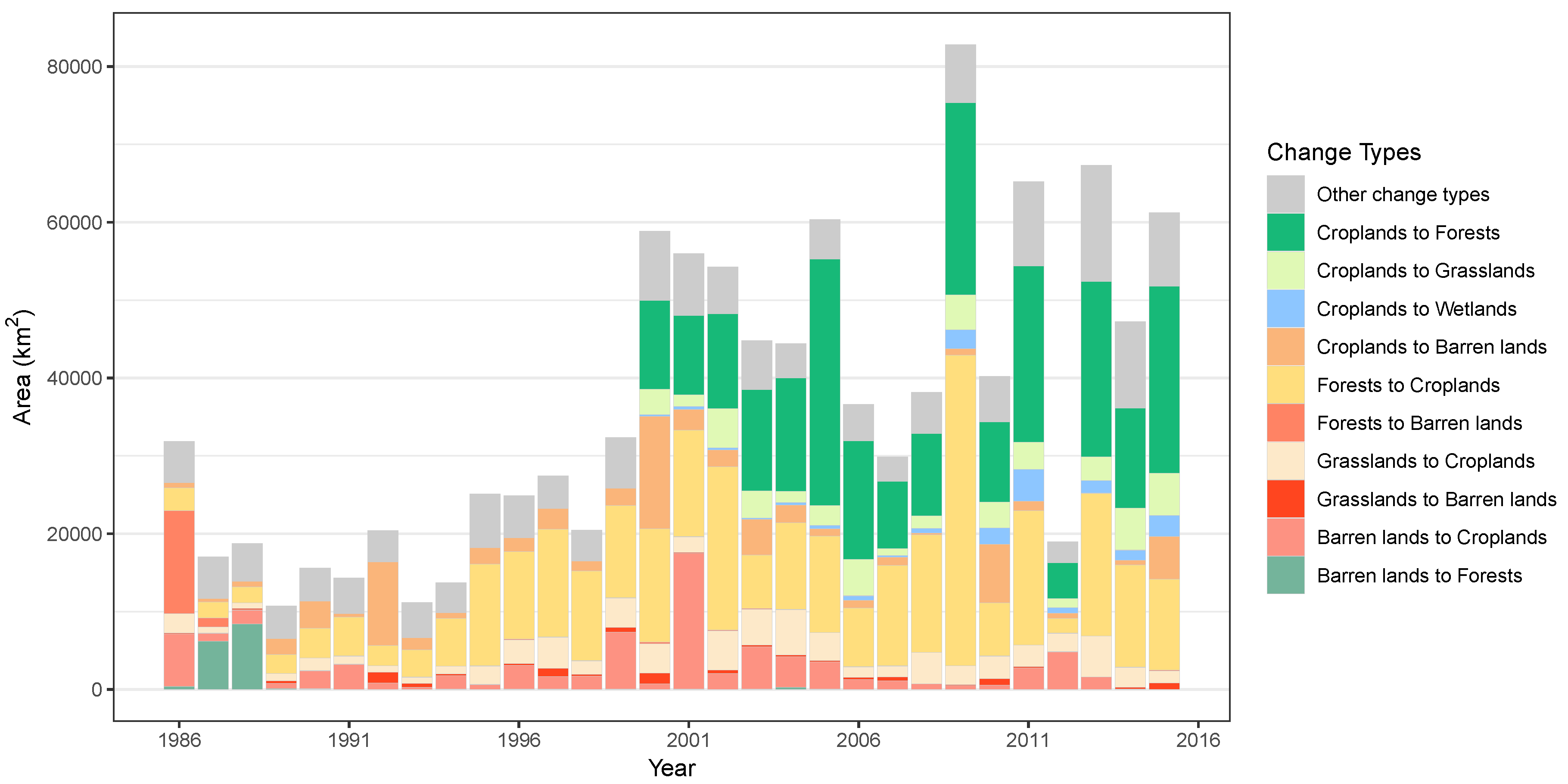
4.2. Land Cover Changes of Northeast China
4.3. Application Highlights
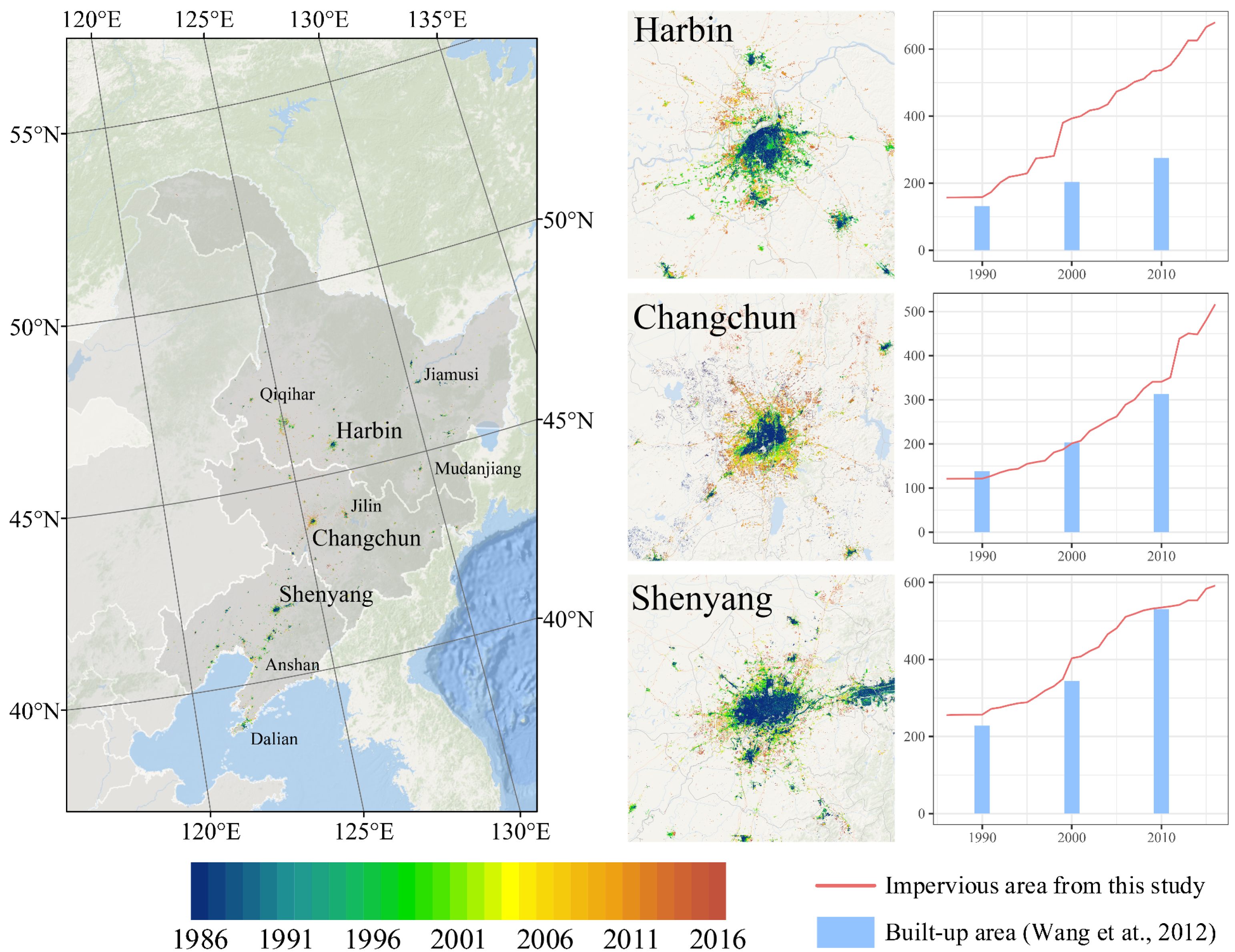
4.3.1. Impervious Surface Cover Changes
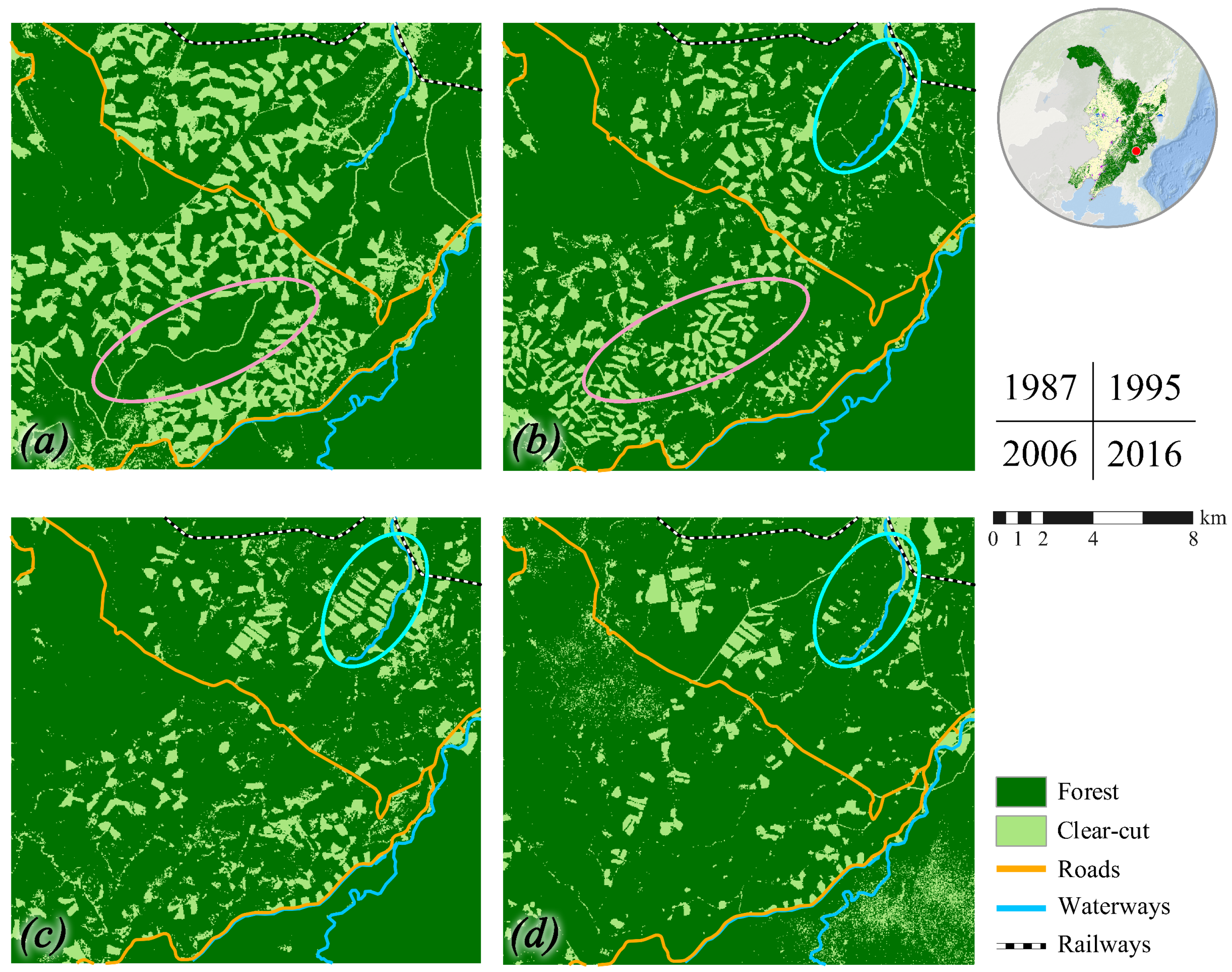
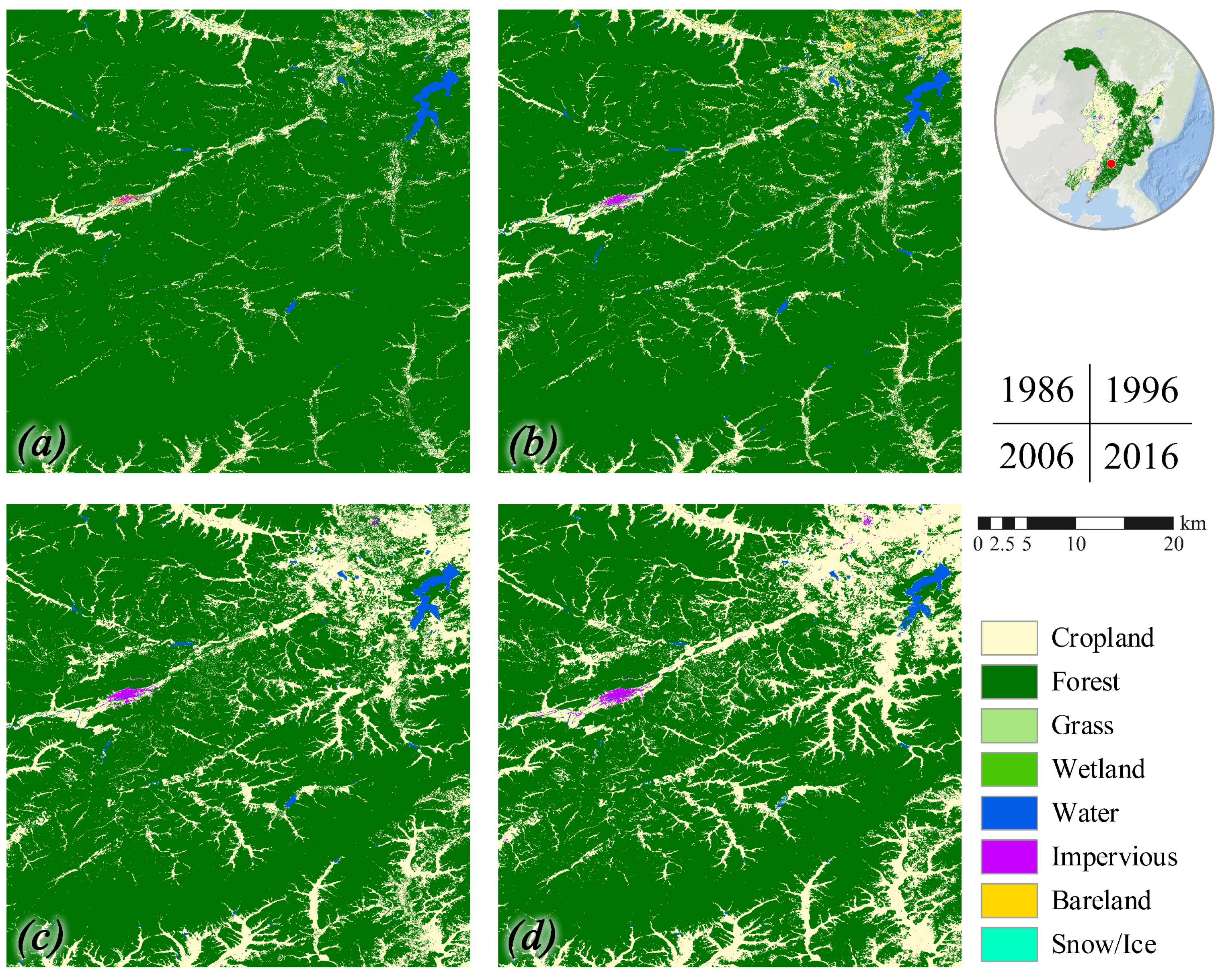
4.3.2. Forest Cover Changes
5. Discussion and Conclusions
Author Contributions
Funding
Conflicts of Interest
References
- Li, B.; Fang, X.; Ye, Y.; Zhang, X. Carbon emissions induced by cropland expansion in Northeast China during the past 300 years. Sci. China Earth Sci. 2014, 57, 2259–2268. [Google Scholar] [CrossRef]
- Zhu, Z.; Sun, X.; Dong, Y.; Zhao, F.; Meixner, F.X. Diurnal variation of ozone flux over corn field in Northwestern Shandong Plain of China. Sci. China Earth Sci. 2014, 57, 503. [Google Scholar] [CrossRef]
- Sun, M.; Zhang, Y.; Ma, J.; Yuan, W.; Li, X.; Cheng, X. Satellite data based estimation of methane emissions from rice paddies in the Sanjiang Plain in Northeast China. PLoS ONE 2017, 12, e0176765. [Google Scholar] [CrossRef] [PubMed]
- Hou, X. Vegetation atlas of China. In Chinese Academy of Science, the Editorial Board of Vegetation Map of China; Science Press: Beijing, China, 2001. [Google Scholar]
- Qian, H.; Yuan, X.Y.; Chou, Y.L. Forest vegetation of Northeast China. In Forest Vegetation of Northeast Asia; Springer: Dordrecht, The Netherlands, 2003; pp. 181–230. [Google Scholar]
- Fang, J.; Chen, A.; Peng, C.; Zhao, S.; Ci, L. Changes in forest biomass carbon storage in China between 1949 and 1998. Science 2001, 292, 2320–2322. [Google Scholar] [CrossRef] [PubMed]
- Piao, S.; Fang, J.; Ciais, P.; Peylin, P.; Huang, Y.; Sitch, S.; Wang, T. The carbon balance of terrestrial ecosystems in China. Nature 2009, 458, 1009–1013. [Google Scholar] [CrossRef] [PubMed]
- Meng, L.; Zhang, L.; Li, Y.; Feng, Z. Land covers and their changes in the Amur tiger distribution regions in China and Russia. In Food Hygiene, Agriculture and Animal Science: Proceedings of the 2015 International Conference on Food Hygiene, Agriculture and Animal Science; World Scientific: Hubei, China, 2016; pp. 293–299. [Google Scholar]
- Luan, X.; Qu, Y.; Li, D.; Liu, S.; Wang, X.; Wu, B.; Zhu, C. Habitat evaluation of wild Amur tiger (Panthera tigris altaica) and conservation priority setting in north-eastern China. J. Environ. Manag. 2011, 92, 31–42. [Google Scholar]
- Zhang, P. Revitalizing old industrial base of Northeast China: Process, policy and challenge. Chin. Geogr. Sci. 2008, 18, 109–118. [Google Scholar] [CrossRef]
- Tan, M. Urban growth and rural transition in China based on DMSP/OLS nighttime light data. Sustainability 2015, 7, 8768–8781. [Google Scholar] [CrossRef]
- Homer, C.; Dewitz, J.; Fry, J.; Coan, M.; Hossain, N.; Larson, C.; Herold, N.; McKerrow, A.; VanDriel, J.N.; Wickham, J. Completion of the 2001 national land cover database for the counterminous United States. Photogramm. Eng. Remote Sens. 2007, 73, 337. [Google Scholar]
- Wickham, J.D.; Stehman, S.V.; Gass, L.; Dewitz, J.; Fry, J.A.; Wade, T.G. Accuracy assessment of NLCD 2006 land cover and impervious surface. Remote Sens. Environ. 2013, 130, 294–304. [Google Scholar] [CrossRef]
- Gong, P.; Wang, J.; Yu, L.; Zhao, Y.; Zhao, Y.; Liang, L.; Niu, Z.; Huang, X.; Fu, H.; Liu, S.; et al. Finer resolution observation and monitoring of global land cover: First mapping results with Landsat TM and ETM+ data. Int. J. Remote Sens. 2013, 34, 2607–2654. [Google Scholar] [CrossRef]
- Feng, D.; Zhao, Y.; Yu, L.; Li, C.; Wang, J.; Clinton, N.; Bai, Y.; Belward, A.; Zhu, Z.; Gong, P. Circa 2014 African land-cover maps compatible with FROM-GLC and GLC2000 classification schemes based on multi-seasonal Landsat data. Int. J. Remote Sens. 2016, 37, 4648–4664. [Google Scholar] [CrossRef]
- Hansen, M.C.; Stehman, S.V.; Potapov, P.V. Quantification of global gross forest cover loss. Proc. Natl. Acad. Sci. USA 2010, 107, 8650–8655. [Google Scholar] [CrossRef] [Green Version]
- Hansen, M.C.; Potapov, P.V.; Moore, R.; Hancher, M.; Turubanova, S.; Tyukavina, A.; Thau, D.; Stehman, S.; Goetz, S.; Loveland, T.R.; et al. High-resolution global maps of 21st-century forest cover change. Science 2013, 342, 850–853. [Google Scholar] [CrossRef]
- Potapov, P.V.; Turubanova, S.; Tyukavina, A.; Krylov, A.; McCarty, J.; Radeloff, V.; Hansen, M. Eastern Europe’s forest cover dynamics from 1985 to 2012 quantified from the full Landsat archive. Remote Sens. Environ. 2015, 159, 28–43. [Google Scholar] [CrossRef]
- Ruelland, D.; Dezetter, A.; Puech, C.; Ardoin-Bardin, S. Long-term monitoring of land cover changes based on Landsat imagery to improve hydrological modelling in West Africa. Int. J. Remote Sens. 2008, 29, 3533–3551. [Google Scholar] [CrossRef]
- Lyons, M.B.; Phinn, S.R.; Roelfsema, C.M. Long term land cover and seagrass mapping using Landsat and object-based image analysis from 1972 to 2010 in the coastal environment of South East Queensland, Australia. ISPRS J. Photogramm. Remote Sens. 2012, 71, 34–46. [Google Scholar] [CrossRef]
- Liu, Y.; Wang, D.; Gao, J.; Deng, W. Land use/cover changes, the environment and water resources in Northeast China. Environ. Manag. 2005, 36, 691–701. [Google Scholar] [CrossRef] [PubMed]
- Gao, J.; Liu, Y.; Chen, Y. Land cover changes during agrarian restructuring in Northeast China. Appl. Geogr. 2006, 26, 312–322. [Google Scholar] [CrossRef]
- Chen, L.; Ren, C.; Zhang, B.; Wang, Z.; Liu, M. Quantifying urban land sprawl and its driving forces in Northeast China from 1990 to 2015. Sustainability 2018, 10, 188. [Google Scholar] [CrossRef]
- Sexton, J.O.; Urban, D.L.; Donohue, M.J.; Song, C. Long-term land cover dynamics by multi-temporal classification across the Landsat-5 record. Remote Sens. Environ. 2013, 128, 246–258. [Google Scholar] [CrossRef]
- Roy, D.P.; Kovalskyy, V.; Zhang, H.; Vermote, E.F.; Yan, L.; Kumar, S.; Egorov, A. Characterization of Landsat-7 to Landsat-8 reflective wavelength and normalized difference vegetation index continuity. Remote Sens. Environ. 2016, 185, 57–70. [Google Scholar] [CrossRef] [Green Version]
- Croft, T.A. Nighttime images of the earth from space. Sci. Am. 1978, 239, 86–98. [Google Scholar] [CrossRef]
- Rouse, J.W.; Haas, R.H.; Schell, J.A.; Deering, D.W. Monitoring Vegetation Systems in the Great Okains with ERTS. In Third Earth Resources Technology Satellite-1 Symposium; Texas A&M Univ.: College Station, TX, USA, 1973; Volume 1, pp. 325–333. [Google Scholar]
- Tucker, C.J. Red and photographic infrared linear combinations for monitoring vegetation. Remote Sens. Environ. 1979, 8, 127–150. [Google Scholar] [CrossRef] [Green Version]
- Liu, H.Q.; Huete, A. A feedback based modification of the NDVI to minimize canopy background and atmospheric noise. IEEE Trans. Geosci. Remote Sens. 1995, 33, 457–465. [Google Scholar]
- Kaufman, Y.J.; Tanre, D. Atmospherically resistant vegetation index (ARVI) for EOS-MODIS. IEEE Trans. Geosci. Remote Sens. 1992, 30, 261–270. [Google Scholar] [CrossRef]
- Huete, A.R. A soil-adjusted vegetation index (SAVI). Remote Sens. Environ. 1988, 25, 295–309. [Google Scholar] [CrossRef]
- Xu, H. Modification of normalised difference water index (NDWI) to enhance open water features in remotely sensed imagery. Int. J. Remote Sens. 2006, 27, 3025–3033. [Google Scholar] [CrossRef]
- Gao, B.C. NDWI—A normalized difference water index for remote sensing of vegetation liquid water from space. Remote Sens. Environ. 1996, 58, 257–266. [Google Scholar] [CrossRef]
- Garcia, M.L.; Caselles, V. Mapping burns and natural reforestation using Thematic Mapper data. Geocarto Int. 1991, 6, 31–37. [Google Scholar] [CrossRef]
- Key, C.H.; Benson, N.C. The Normalized Burn Ratio (NBR): A Landsat TM Radiometric Measure of Burn Severity; United States Geological Survey, Northern Rocky Mountain Science Center: Bozeman, MT, USA, 1999.
- Li, X.; Gong, P.; Liang, L. A 30-year (1984–2013) record of annual urban dynamics of Beijing City derived from Landsat data. Remote Sens. Environ. 2015, 166, 78–90. [Google Scholar] [CrossRef]
- Xu, Y.; Yu, L.; Zhao, Y.; Feng, D.; Cheng, Y.; Cai, X.; Gong, P. Monitoring cropland changes along the Nile River in Egypt over past three decades (1984–2015) using remote sensing. Int. J. Remote Sens. 2017, 38, 4459–4480. [Google Scholar] [CrossRef]
- Faostat. Food and agriculture organization of the United Nations. Stat. Database. 2013. Available online: http://www.fao.org/faostat/en/#data (accessed on 3 March 2019).
- Liu, J.; Liu, M.; Tian, H.; Zhuang, D.; Zhang, Z.; Zhang, W.; Tang, X.; Deng, X. Spatial and temporal patterns of China’s cropland during 1990–2000: An analysis based on Landsat TM data. Remote Sens. Environ. 2005, 98, 442–456. [Google Scholar] [CrossRef]
- Liu, J.; Kuang, W.; Zhang, Z.; Xu, X.; Qin, Y.; Ning, J.; Zhou, W.; Zhang, S.; Li, R.; Yan, C.; et al. Spatiotemporal characteristics, patterns, and causes of land-use changes in China since the late 1980s. J. Geogr. Sci. 2014, 24, 195–210. [Google Scholar] [CrossRef]
- Schneider, A. Monitoring land cover change in urban and peri-urban areas using dense time stacks of Landsat satellite data and a data mining approach. Remote Sens. Environ. 2012, 124, 689–704. [Google Scholar] [CrossRef]
- Mertes, C.M.; Schneider, A.; Sulla-Menashe, D.; Tatem, A.; Tan, B. Detecting change in urban areas at continental scales with MODIS data. Remote Sens. Environ. 2015, 158, 331–347. [Google Scholar] [CrossRef] [Green Version]
- Zhao, Y.; Gong, P.; Yu, L.; Hu, L.; Li, X.; Li, C.; Zhang, H.; Zheng, Y.; Wang, J.; Zhao, Y.; et al. Towards a common validation sample set for global land-cover mapping. Int. J. Remote Sens. 2014, 35, 4795–4814. [Google Scholar] [CrossRef] [Green Version]
- Wang, L.; Li, C.; Ying, Q.; Cheng, X.; Wang, X.; Li, X.; Hu, L.; Liang, L.; Yu, L.; Huang, H.; et al. China’s urban expansion from 1990 to 2010 determined with satellite remote sensing. Chin. Sci. Bull. 2012, 57, 2802–2812. [Google Scholar] [CrossRef] [Green Version]
- Yu, D.; Zhou, L.; Zhou, W.; Ding, H.; Wang, Q.; Wang, Y.; Wu, X.; Dai, L. Forest management in Northeast China: History, problems, and challenges. Environ. Manag. 2011, 48, 1122–1135. [Google Scholar] [CrossRef] [PubMed]
- Wang, Z.; Fu, P.; Deng, Y. Founder and pioneer of China’s Botany and Ecology—In memory of 100th anniversary of Liu Shen’e‘s birth. Chin. J. Ecol. 1997, 16, 77–80. [Google Scholar]
- Liu, S. Comprehending the Forest Cutting and Regeneration Regulation from the Situation of Cutting and Regeneration of Korean Pine in Northeast China; Wang Z(ed) (1985) Liu Shen’E Collect Works; Science Press: Beijing, China, 1973; pp. 314–326. [Google Scholar]
- Xu, J.; Tao, R.; Amacher, G.S. An empirical analysis of China’s state-owned forests. For. Policy Econ. 2004, 6, 379–390. [Google Scholar] [CrossRef]
- Olofsson, P.; Foody, G.M.; Stehman, S.V.; Woodcock, C.E. Making better use of accuracy data in land change studies: Estimating accuracy and area and quantifying uncertainty using stratified estimation. Remote Sens. Environ. 2013, 129, 122–131. [Google Scholar] [CrossRef]
- Gray, J.; Song, C. Consistent classification of image time series with automatic adaptive signature generalization. Remote Sens. Environ. 2013, 134, 333–341. [Google Scholar] [CrossRef]
- Corcoran, J.M.; Knight, J.F.; Gallant, A.L. Influence of multi-source and multi-temporal remotely sensed and ancillary data on the accuracy of random forest classification of wetlands in Northern Minnesota. Remote Sens. 2013, 5, 3212–3238. [Google Scholar] [CrossRef]
- Dannenberg, M.P.; Hakkenberg, C.R.; Song, C. Consistent classification of Landsat time series with an improved automatic adaptive signature generalization algorithm. Remote Sens. 2016, 8, 691. [Google Scholar] [CrossRef]
- Southworth, J.; Munroe, D.; Nagendra, H. Land cover change and landscape fragmentation—Comparing the utility of continuous and discrete analyses for a western Honduras region. Agric. Ecosyst. Environ. 2004, 101, 185–205. [Google Scholar] [CrossRef]
- Zhao, Y.; Feng, D.; Yu, L.; Wang, X.; Chen, Y.; Bai, Y.; Hernández, H.J.; Galleguillos, M.; Estades, C.; Biging, G.S.; et al. Detailed dynamic land cover mapping of Chile: Accuracy improvement by integrating multi-temporal data. Remote Sens. Environ. 2016, 183, 170–185. [Google Scholar] [CrossRef]


| Code | Land Cover Type |
|---|---|
| 10 | Croplands (CR) |
| 20 | Forests/Shrubs (FS) |
| 30 | Grasslands (GR) |
| 50 | Wetlands (WE) |
| 60 | Water bodies (WB) |
| 80 | Impervious surfaces (IS) |
| 90 | Barren lands (BL) |
| 100 | Snow/Ice (SI) |
| 120 | Clouds (CL) |
| Prediction | |||||||||
|---|---|---|---|---|---|---|---|---|---|
| Croplands | Forests/Shrubs | Grasslands | Wetlands | Water Bodies | Impervious | Bare Lands | Producer’s Accuracy (%) | ||
| Reference | Croplands | 70 | 3 | 0 | 0 | 0 | 0 | 0 | 95.89 |
| Forests/Shrubs | 7 | 87 | 0 | 0 | 0 | 0 | 0 | 92.55 | |
| Grasslands | 0 | 0 | 4 | 0 | 0 | 0 | 0 | 100.00 | |
| Wetlands | 10 | 3 | 1 | 1 | 1 | 0 | 0 | 6.25 | |
| Water bodies | 3 | 2 | 2 | 0 | 25 | 1 | 0 | 75.76 | |
| Impervious | 12 | 0 | 1 | 0 | 1 | 17 | 2 | 51.52 | |
| Bare lands | 1 | 0 | 0 | 0 | 0 | 0 | 5 | 83.33 | |
| User’s accuracy (%) | 67.96 | 91.58 | 50.00 | 100.00 | 92.59 | 94.44 | 71.43 | 80.69 | |
| Prediction | |||||||||
|---|---|---|---|---|---|---|---|---|---|
| Croplands | Forests/Shrubs | Grasslands | Wetlands | Water Bodies | Impervious | Bare Lands | Producer’s Accuracy (%) | ||
| Reference | Croplands | 100 | 2 | 2 | 0 | 0 | 0 | 0 | 96.15 |
| Forests/Shrubs | 9 | 106 | 0 | 0 | 0 | 0 | 0 | 92.17 | |
| Grasslands | 0 | 1 | 8 | 0 | 0 | 0 | 0 | 88.89 | |
| Wetlands | 5 | 0 | 0 | 13 | 4 | 0 | 0 | 59.09 | |
| Water bodies | 0 | 1 | 0 | 2 | 34 | 1 | 0 | 89.47 | |
| Impervious | 7 | 1 | 0 | 0 | 1 | 24 | 2 | 68.57 | |
| Bare lands | 0 | 0 | 0 | 0 | 0 | 0 | 4 | 100.00 | |
| User’s accuracy (%) | 82.64 | 95.50 | 80.00 | 86.67 | 87.18 | 96.00 | 66.67 | 88.38 | |
© 2019 by the authors. Licensee MDPI, Basel, Switzerland. This article is an open access article distributed under the terms and conditions of the Creative Commons Attribution (CC BY) license (http://creativecommons.org/licenses/by/4.0/).
Share and Cite
Zhao, Y.; Feng, D.; Yu, L.; Cheng, Y.; Zhang, M.; Liu, X.; Xu, Y.; Fang, L.; Zhu, Z.; Gong, P. Long-Term Land Cover Dynamics (1986–2016) of Northeast China Derived from a Multi-Temporal Landsat Archive. Remote Sens. 2019, 11, 599. https://0-doi-org.brum.beds.ac.uk/10.3390/rs11050599
Zhao Y, Feng D, Yu L, Cheng Y, Zhang M, Liu X, Xu Y, Fang L, Zhu Z, Gong P. Long-Term Land Cover Dynamics (1986–2016) of Northeast China Derived from a Multi-Temporal Landsat Archive. Remote Sensing. 2019; 11(5):599. https://0-doi-org.brum.beds.ac.uk/10.3390/rs11050599
Chicago/Turabian StyleZhao, Yuanyuan, Duole Feng, Le Yu, Yuqi Cheng, Meinan Zhang, Xiaoxuan Liu, Yidi Xu, Lei Fang, Zhiliang Zhu, and Peng Gong. 2019. "Long-Term Land Cover Dynamics (1986–2016) of Northeast China Derived from a Multi-Temporal Landsat Archive" Remote Sensing 11, no. 5: 599. https://0-doi-org.brum.beds.ac.uk/10.3390/rs11050599