Tight Fusion of a Monocular Camera, MEMS-IMU, and Single-Frequency Multi-GNSS RTK for Precise Navigation in GNSS-Challenged Environments

Abstract

Precise position, velocity, and attitude is essential for self-driving cars and unmanned aerial vehicles (UAVs). The integration of global navigation satellite system (GNSS) real-time kinematics (RTK) and inertial measurement units (IMUs) is able to provide high-accuracy navigation solutions in open-sky conditions, but the accuracy will be degraded severely in GNSS-challenged environments, especially integrated with the low-cost microelectromechanical system (MEMS) IMUs. In order to navigate in GNSS-denied environments, the visual–inertial system has been widely adopted due to its complementary characteristics, but it suffers from error accumulation. In this contribution, we tightly integrate the raw measurements from the single-frequency multi-GNSS RTK, MEMS-IMU, and monocular camera through the extended Kalman filter (EKF) to enhance the navigation performance in terms of accuracy, continuity, and availability. The visual measurement model from the well-known multistate constraint Kalman filter (MSCKF) is combined with the double-differenced GNSS measurement model to update the integration filter. A field vehicular experiment was carried out in GNSS-challenged environments to evaluate the performance of the proposed algorithm. Results indicate that both multi-GNSS and vision contribute significantly to the centimeter-level positioning availability in GNSS-challenged environments. Meanwhile, the velocity and attitude accuracy can be greatly improved by using the tightly-coupled multi-GNSS RTK/INS/Vision integration, especially for the yaw angle.

1. Introduction

Precise navigation is a fundamental module for a wide range of applications such as autonomous driving, unmanned aerial vehicles (UAVs), and mobile mapping [1,2]. For centimeter-level high-accuracy positioning of the global positioning system (GPS), the carrier phase integer ambiguities have to be resolved correctly [3]. It has been shown that the dual-frequency GPS real-time kinematics (RTK) can achieve rapid or even instantaneous ambiguity resolution (AR) for short baselines under open-sky conditions [4]. By contrast, the single-frequency GPS RTK has a low AR success rate due to the short wavelength of the $f_1$ frequency and the unmodeled errors in the measurements, such as the multipath, especially in dynamic environments [5]. Compared with the dual-frequency receivers, the single-frequency receivers are preferred for applications such as microaerial vehicles due to the low-cost and low power consumption requirements. Recent research has shown that the performance of the GPS single-frequency RTK can be improved substantially by using the multiconstellation global navigation satellite system (multi-GNSS), including the Chinese BeiDou navigation satellite system (BDS), the Russian GLObal NAvigation Satellite System (GLONASS), and the European Galileo navigation satellite system [4,6,7,8,9].

As the positioning performance of GNSS depends on the continuous tracking of the passible radio signal, the positioning performance of GNSS in terms of accuracy, availability, and continuity will be degraded in GNSS-challenged environments. However, the demand for high-precision navigation performance has been increasing in urban environments where GNSS signals suffer from frequent blockages. In order to improve the positioning capability in such conditions, the integration of GNSS and an inertial navigation system (INS) is adopted widely to provide continuous position, velocity, and attitude [10,11,12,13]. With the advances in microelectromechanical system (MEMS) inertial sensor technology, the low-cost GNSS/MEMS-IMU (inertial measurement units) integration becomes attractive to provide navigation solutions [14,15,16]. However, the main drawback of low-cost MEMS-IMU is that its navigation error will diverge rapidly in a short time in the absence of effective GNSS measurements.

In order to provide navigation information for vehicles in GPS-denied environments, the integration of a monocular camera and MEMS-IMU has gained wide interest in the robotics community owing to their complementary characteristics and low-cost hardware. On one hand, the IMU can recover the metric scale of the monocular vision and greatly improve the motion tracking performance. On the other hand, the visual measurements can greatly limit the error drift of the low-cost MEMS-IMU. The visual–inertial fusion algorithms are either based on the extended Kalman filter (EKF) [17,18,19,20] or utilizing iterative minimization over a bounded-size sliding window of recent states [21,22,23]. The latter method is generally considered to have higher estimation accuracy, as it uses iterative linearization to deal with nonlinearity. However, this method has a high computational cost due to the multiple iterations in comparison with the filter-based methods. A well-known filter-based visual–inertial odometry (VIO) approach is the multistate constraint Kalman filter (MSCKF), which is able to achieve comparable estimation accuracy, but has lower computational cost [17,18]. It maintains a sliding window of camera poses in the state vector instead of feature points, and thus the computational complexity is only linear in the number of features.

Although the VIO or visual–inertial simultaneous localization and mapping (VI-SLAM) can provide accurate pose estimation, the absolute position and attitude information in a global reference system cannot be obtained and the accumulated drifts are unavoidable over time. The integration with GNSS can overcome this limitation easily, and the multisensor fusion concept has been increasingly accepted to provide robust, accurate, and continuous navigation solutions [24]. In [25,26,27], a visual sensor was used to aid the GNSS/INS integration to provide navigation solutions in GNSS-challenged environments. Oskiper et al. developed a multisensor navigation algorithm using a GPS, IMU, and monocular camera for augmented reality [28]. Vu et al. used computer vision, differential pseudorange GPS measurements, and mapped landmarks to aid the INS to provide lane-level vehicle navigation with high availability and integrity [29]. In [30], a generic multisensor fusion EKF was presented to fuse the visual and inertial sensors and GPS position measurements to obtain drift-free pose estimates. Shepard et al. incorporated the carrier phase differential GPS position measurements into the bundle-adjustment based visual SLAM framework to obtain high-precision globally referenced position and velocity [31]. More recently, the local VIO poses have been fused with GPS position measurements to infer the global six-degrees-of-freedom (DoF) pose using a graph-optimization-based multisensor fusion approach [32]. The alignment transformation between the local frame and global frame is continuously updated during the optimization, which leads to extra computation.

Although the fusion of the GPS, IMU, and camera has been investigated in several previous studies, they mainly used the GPS position or pseudorange measurements, and the related algorithms were validated using simulated data or under open-sky conditions. In order to make the most of their complementary properties for precise navigation in GNSS-constrained environments, the visual and inertial measurements should be utilized to aid the GNSS positioning as well. In this contribution, we first tightly integrate the single-frequency multi-GNSS RTK, MEMS-IMU, and the monocular camera to enhance the navigation performance in terms of accuracy, continuity, and availability in GNSS-challenged environments. A field vehicular experiment was conducted at Wuhan University to evaluate the performance of the proposed algorithm. The benefits of multi-GNSS and visual data for the derived position, velocity, and attitude are analyzed.

The remaining paper is organized as follows: Section 2 presents the tightly coupled multi-GNSS RTK/INS/Vision integration models including the error state model, GNSS measurement model, visual measurement model, and ambiguity resolution with inertial aiding. Then, the field test and data processing strategies are described in Section 3. In Section 4, the experimental results are presented and analyzed. Finally, discussions about the results and some conclusions are given in Section 5 and Section 6, respectively.

2. Methods

The EKF has been shown to be a popular tool for multisensor fusion. In this research, the EKF directly fuses the data from the multi-GNSS, MEMS-IMU, and monocular camera to obtain optimal estimates of the integrated system state. In order to present the tightly coupled integration algorithm, the error state model, the multi-GNSS measurement model, the visual measurement model, and the INS-aided single-epoch ambiguity resolution approach are introduced.

2.1. Error State Model

In this research, the inertial system is mechanized in the $e$-frame (i.e., Earth-centered Earth-fixed, ECEF). The mechanization in the $e$-frame makes it easier to use the raw GNSS observables and more efficient than the local-level equivalent algorithm. The INS dynamic model is constructed as the $\varphi$-angle error model, which can be described in the $e$-frame as follows [33]:

$$\{\begin{array}{c}\delta {\dot{\mathit{p}}}_{eb}^e=\delta {\mathit{v}}_{eb}^e\\ \delta {\dot{\mathit{v}}}_{eb}^e=\left({\mathit{R}}_b^e{\mathit{f}}^b\right)\times \delta {\mathit{\varphi }}_{be}^e+{\mathit{R}}_b^e\delta {\mathit{f}}^b-2{\mathit{\omega }}_{ie}^e\times \delta {\mathit{v}}_{eb}^e+\delta {\mathit{g}}^e\\ \delta {\dot{\mathit{\varphi }}}_{be}^e=-({\mathit{\omega }}_{ie}^e\times )\delta {\mathit{\varphi }}_{be}^e-{\mathit{R}}_b^e\delta {\mathit{\omega }}_{ib}^b\end{array}$$

(1)

where $\delta {\dot{\mathit{p}}}_{eb}^e$, $\delta {\dot{\mathit{v}}}_{eb}^e$, and $\delta {\dot{\mathit{\varphi }}}_{be}^e$ denote the derivative of position, velocity, and attitude error, respectively; ${\mathit{R}}_b^e$ is the rotation matrix from the body ($b$) frame (i.e., forward–right–down, FRD) to the $e$-frame; ${\mathit{f}}^b$ denotes the specific force in the $b$-frame; ${\mathit{\omega }}_{ie}^e$ denotes the angular rate of the $e$-frame with respect to the inertial ($i$) frame, projected to the $e$-frame;$\delta {\mathit{g}}^e$ denotes the gravity vector in the $e$-frame; and $\delta {\mathit{f}}^b$ and $\delta {\mathit{\omega }}_{ib}^b$ are the errors of the accelerometer and gyroscope, respectively.

In order to model the bias error of low-cost MEMS-IMUs, the gyroscope and accelerometer bias error are augmented into the filter state and estimated online. Generally, they are modeled as a first-order Gauss–Markov process [34]:

$$\left[\begin{array}{c}\delta {\dot{\mathit{b}}}_g\\ \delta {\dot{\mathit{b}}}_a\end{array}\right]=\left[\begin{array}{c}-\frac{1}{{\tau }_{b_g}}\delta {\mathit{b}}_g\\ -\frac{1}{{\tau }_{b_a}}\delta {\mathit{b}}_a\end{array}\right]+\mathit{w}$$

(2)

where $\delta {\mathit{b}}_g$ and $\delta {\mathit{b}}_a$ are the bias error of the gyroscope and accelerometer, respectively; ${\tau }_{b_g}$ and ${\tau }_{b_a}$ are the corresponding correlation time of the first-order Gauss–Markov process; and $\mathit{w}$ is the driving white noise.

For the multistate constraint Kalman filter model, the error states of a sliding window of poses are augmented into the filter state vector. Every time a new image is recorded, the state vector is augmented with a copy of the current IMU pose. Therefore, the error state vector at $t_k$ can be written as:

$$\delta {\mathit{x}}_k=\left[\begin{array}{cccccc}\delta {\mathit{x}}_{IMU}^T& \delta {\mathit{\varphi }}_1^T& \delta {\mathit{p}}_1^T& \cdots & \delta {\mathit{\varphi }}_K^T& \delta {\mathit{p}}_K^T\end{array}\right]$$

(3)

with

$$\delta {\mathit{x}}_{IMU}={\left[\begin{array}{ccccc}\delta {\mathit{p}}_k^T& \delta {\mathit{v}}_k^T& \delta {\mathit{\varphi }}_k^T& \delta {\mathit{b}}_a^T& \delta {\mathit{b}}_g^T\end{array}\right]}^T$$

(4)

where $\delta {\mathit{\varphi }}_i$ and $\delta {\mathit{p}}_i$, $i=1\cdots K$ are the error states of the IMU attitude and position, respectively; and $K$ denotes the total number of poses in the sliding window.

2.2. Double-Differenced Measurement Model of the GPS/BeiDou/GLONASS System

In the single-frequency RTK positioning, the pseudorange and carrier phase observations on the $f_1$ frequency will be used together. Since the $f_1$ frequencies from the GPS, BDS, and GLONASS satellites are different, the double-differencing (DD) formulation should be applied within the individual GNSS system [6]. The double-differenced code and phase observation equations for a single GNSS system can be written as:

$$\nabla \Delta P=\nabla \Delta \rho +\nabla \Delta T+\nabla \Delta I+\nabla \Delta {\epsilon }_P$$

(5)

$$\mathsf{\lambda }\nabla \Delta \mathit{\phi }=\nabla \Delta \rho +\nabla \Delta T-\nabla \Delta I+\mathsf{\lambda }\nabla \Delta N+\nabla \Delta {\epsilon }_{\mathit{\phi }}$$

(6)

where $\nabla \Delta (·)$ denotes the DD operator; $P$ and $\mathit{\phi }$ denote the pseudorange and carrier phase observations, respectively; $\rho$ is the geometric distance between the receiver and satellite; $T$ and $I$ denote the tropospheric and ionospheric delay, respectively; $\lambda$ and N are carrier phase wavelength and integer ambiguity, respectively; and ${\epsilon }_P$ and ${\epsilon }_{\mathit{\phi }}$ are the unmodeled residual error (measurement noise, multipath, etc.) of pseudorange and carrier phase observations, respectively.

Different from the GPS and BDS, the GLONASS employs the frequency division multiple access (FDMA) modulation. The FDMA modulation makes GLONASS ambiguity resolution difficult due to the carrier phase interfrequency bias (IFB). The IFB cannot be canceled in the DD process and will prevent the correct integer AR [35]. In this research, we precalibrated the IFB using the method proposed by the authors of [36]. As the frequencies from different GLONASS satellites are different, the DD phase observations $\lambda \nabla \Delta \mathit{\phi }$ and ambiguities $\lambda \nabla \Delta N$ could be rewritten as:

$$\mathsf{\lambda }\nabla \Delta \mathit{\phi }={\lambda }^k\Delta {\mathit{\phi }}^k-{\lambda }^r\Delta {\mathit{\phi }}^r$$

(7)

$$\mathsf{\lambda }\nabla \Delta N={\lambda }^k\mathsf{\Delta }{N}^k-{\lambda }^r\mathsf{\Delta }{N}^r={\lambda }^k\nabla \mathsf{\Delta }{N}^{kr}+({\lambda }^k-{\lambda }^r)\mathsf{\Delta }{N}^r$$

(8)

where the superscripts k and r denote the nonreference and reference satellite, respectively, and $\mathsf{\Delta }(·)$ denotes the single-differenced (SD) operator. In Equation (8), the SD ambiguity can be estimated with the SD code observations [37].

For short baselines in this research, the atmospheric terms $T$ and $I$ in Equations (5) and (6) can be neglected. The remaining unknown parameters in Equations (5) and (6) are the baseline increment vector and integer ambiguities. By linearizing the DD code and phase observation equation with unknown parameters, the error equation can be described in a matrix form as follows:

$$\left[\begin{array}{c}{\mathit{\epsilon }}_P\\ {\mathit{\epsilon }}_{\mathit{\phi }}\end{array}\right]=\left[\begin{array}{cc}\mathit{H}& {\mathbf{0}}_{n\times n}\\ \mathit{H}& \Lambda \end{array}\right]\left[\begin{array}{c}\delta {\mathit{p}}_r\\ \nabla \Delta \mathit{N}\end{array}\right]-\left[\begin{array}{c}\nabla \Delta P-\nabla \Delta {\mathit{r}}_0\\ \mathsf{\lambda }\nabla \Delta \mathit{\phi }-\nabla \Delta {\mathit{r}}_0\end{array}\right]$$

(9)

with

$$\mathit{H}={\left[\begin{array}{ccc}{\mathit{H}}^G& {\mathit{H}}^C& {\mathit{H}}^R\end{array}\right]}^T$$

(10)

$$\Lambda =diag\left(\begin{array}{ccc}{\Lambda }^G& {\Lambda }^C& {\Lambda }^R\end{array}\right)$$

(11)

$$\mathit{N}={\left[\begin{array}{ccc}{\mathit{N}}^G& {\mathit{N}}^C& {\mathit{N}}^R\end{array}\right]}^T$$

(12)

where the superscripts ‘G’, ‘C’, and ‘R’ represent GPS, BeiDou, and GLONASS, respectively; $n$ is the total number of DD ambiguities from the combined GPS, BeiDou, and GLONSS systems; $\mathsf{\delta }{\mathit{p}}_r$ denotes the baseline increment vector; $\nabla \Delta {\mathit{r}}_0$ is the computed DD range with the approximate rover coordinate and satellite position; $\mathit{H}$ is the design matrix; and $\Lambda$ contains the wavelengths of the $f_1$ frequency corresponding to the different individual GPS, BeiDou, and GLONASS satellites.

For the tightly coupled integration, the measurement vector ${\mathit{Z}}_k$ is calculated by:

$${\mathit{Z}}_k=\left[\begin{array}{c}\nabla \Delta {\widehat{\mathit{\rho }}}_{INS}-\nabla \Delta {\mathit{P}}_{GNSS}\\ \nabla \Delta {\widehat{\mathit{\rho }}}_{INS}-\lambda \nabla \Delta {\mathit{\phi }}_{GNSS}\end{array}\right]$$

(13)

where $\nabla \Delta {\widehat{\rho }}_{INS}$ represents the INS-derived DD geometric range $\nabla \Delta P_{GNSS}$ and $\nabla \Delta {\mathit{\phi }}_{GNSS}$ are the raw GNSS DD code and phase observations, respectively. Since the IMU center and GNSS antenna cannot be installed at the same position, the lever-arm correction should be applied, which can be written in the $e$-frame as:

$${\mathit{r}}_{GNSS}^e={\mathit{r}}_{IMU}^e+{\mathit{R}}_b^e{\mathbf{\ell }}_{GNSS}^b$$

(14)

where ${\mathit{r}}_{GNSS}^e$ and ${\mathit{r}}_{IMU}^e$ are the position of the GNSS antenna and IMU in the $e$-frame, respectively; ${\mathit{R}}_b^e$ is the rotation matrix from the $b$-frame to the $e$-frame; and ${\mathit{\ell }}_{GNSS}^b$ is the lever-arm offset in the $b$-frame.

The position error between the GNSS antenna and the IMU center can be derived after the error perturbation analysis of Equation (14):

$$\delta {\mathit{r}}_{GNSS}^e\approx \delta {\mathit{r}}_{IMU}^e+\left[{\mathit{R}}_b^e{\mathit{\ell }}_{GNSS}^b\times \right]\delta {\mathit{\varphi }}_{be}^e$$

(15)

where $\times$ is the cross-product operator. The final design matrix for the GNSS measurement update can be derived by combining Equations (5), (6), (10), (13), and (15):

$${\mathit{H}}_{k,GNSS}=\left[\begin{array}{ccccc}\mathit{H}& {\mathbf{0}}_{n\times 3}& \mathit{H}·\left[{\mathit{R}}_b^e{\mathit{\ell }}_{GNSS}^b\times \right]& {\mathbf{0}}_{n\times 6}& {\mathbf{0}}_{n\times 6K}\end{array}\right]$$

(16)

where $n$ is the number of DD code or phase measurements and $K$ is the number of the camera poses in the sliding window.

2.3. Visual Measurement Model

The underlying idea of the well-known MSCKF is that it uses geometric constraints that arise when a static feature is observed from multiple camera poses. In order to present the measurement model clearly, a single static feature, $f_j$, is considered. Assuming that a static feature is observed by camera pose ${\mathit{C}}_i$, the estimated image measurements can be written as:

$${\widehat{\mathit{z}}}_i^{\left(j\right)}=\left[\begin{array}{c}{\widehat{X}}_j^{C_i}/{\widehat{Z}}_j^{C_i}\\ {\widehat{Y}}_j^{C_i}/{\widehat{Z}}_j^{C_i}\end{array}\right]+{\mathit{n}}_i^{\left(j\right)}$$

(17)

where $n_i^{\left(j\right)}$ is the image noise vector and ${\widehat{X}}_j^{C_i}$, ${\widehat{Y}}_j^{C_i}$ and ${\widehat{Z}}_j^{C_i}$ are the feature positions in the camera frame, which can be calculated by:

$${\left[\begin{array}{ccc}{\widehat{X}}_j^{C_i}& {\widehat{Y}}_j^{C_i}& {\widehat{Z}}_j^{C_i}\end{array}\right]}^T={\widehat{\mathit{R}}}_G^{C_i}\left({\widehat{\mathit{p}}}_{f_j}^G-{\widehat{\mathit{p}}}_{C_i}^G\right)$$

(18)

where ${\widehat{\mathit{R}}}_G^{C_i}$ and ${\widehat{\mathit{p}}}_{C_i}^G$ are the attitude rotation matrix and position vector of the camera pose ${\mathit{C}}_i$, respectively, and ${\widehat{\mathit{p}}}_{f_j}^G$ is the estimated feature position in the global frame ($e$-frame), which can be obtained by employing least-squares minimization from multiple camera measurements [17]. Then, the measurement residual can be calculated by:

$${\mathit{r}}_i^{\left(j\right)}={\mathit{z}}_i^{\left(j\right)}-{\widehat{\mathit{z}}}_i^{\left(j\right)}$$

(19)

By linearizing the above equation about the states and the feature position, the residual can be written approximately as:

$${\mathit{r}}_i^{\left(j\right)}\approx {\mathit{H}}_{{\mathit{X}}_i}^{\left(j\right)}\delta {\mathit{x}}_k+{\mathit{H}}_{f_i}^{\left(j\right)}\delta {\mathit{p}}_{f_j}^G+{\mathit{n}}_i^{\left(j\right)}$$

(20)

where ${\mathit{H}}_{{\mathit{X}}_{\mathit{i}}}^{\left(j\right)}$ and ${\mathit{H}}_{f_i}^{\left(j\right)}$ are the Jacobians of the estimated measurement ${\widehat{\mathit{z}}}_i^{\left(j\right)}$ with respect to the state vector and the feature position, respectively, and $\delta {\mathit{p}}_{f_j}^G$ is the error of the estimated feature position. The corresponding Jacobians can be derived as:

$${\mathit{H}}_{{\mathit{X}}_{\mathit{i}}}^{\left(j\right)}=\left[\begin{array}{cccccc}{\mathbf{0}}_{2\times 15}& {\mathbf{0}}_{2\times 6}& \cdots & {\mathit{J}}_i^{\left(j\right)}\left({\widehat{\mathit{X}}}_{f_j}^{C_i}\times \right)& -{\mathit{J}}_i^{\left(j\right)}{\widehat{\mathit{R}}}_G^{C_i}& \cdots \end{array}\right]$$

(21)

$${\mathit{H}}_{f_i}^{\left(j\right)}={\mathit{J}}_i^{\left(j\right)}{\widehat{\mathit{R}}}_G^{C_i}$$

(22)

with

$${\mathit{J}}_i^{\left(j\right)}=\left(1/{\left({\widehat{Z}}_j^{C_i}\right)}^2\right)\left[\begin{array}{ccc}{\widehat{Z}}_j^{C_i}& 0& -{\widehat{X}}_j^{C_i}\\ 0& {\widehat{Z}}_j^{C_i}& -{\widehat{Y}}_j^{C_i}\end{array}\right]$$

(23)

Usually, a static feature will be observed by multiple consecutive camera poses; therefore, the complete residual vector for this feature can be obtained by stacking all the individual residuals together:

$$\underset{{\mathit{r}}^{\left(j\right)}}{\underbrace{\left[\begin{array}{c}{\mathit{r}}_1^{\left(j\right)}\\ ⋮\\ {\mathit{r}}_k^{\left(j\right)}\end{array}\right]}}\approx \underset{{\mathit{H}}_{\mathit{X}}^{\left(j\right)}}{\underbrace{\left[\begin{array}{c}{\mathit{H}}_1^{\left(j\right)}\\ ⋮\\ {\mathit{H}}_k^{\left(j\right)}\end{array}\right]}}\delta {\mathit{x}}_k+\underset{{\mathit{H}}_f^{\left(j\right)}}{\underbrace{\left[\begin{array}{c}{\mathit{H}}_{f,1}^{\left(j\right)}\\ ⋮\\ {\mathit{H}}_{f,k}^{\left(j\right)}\end{array}\right]}}\delta {\mathit{p}}_{f_j}^G+{\mathit{n}}^{\left(j\right)}$$

(24)

where $k$ denotes the $k$-th camera pose in the sliding window.

In order to perform the EKF update, the residuals should be in the form of $\mathit{r}\approx \mathit{H}\delta {\mathit{x}}_k+\mathit{n}$. This can be achieved by projecting the residual vector $r^{\left(j\right)}$ on the left null space of the matrix $H_f^{\left(j\right)}$. Assuming that $A$ is a unitary matrix whose columns form the basis of the left null space of $H_f^{\left(j\right)}$, the residual formula can be rewritten as:

$${\mathit{r}}_o^{\left(j\right)}={\mathit{A}}^T\left({\mathit{z}}^{\left(j\right)}-{\widehat{\mathit{z}}}^{\left(j\right)}\right)={\mathit{A}}^T{\mathit{H}}_X^{\left(j\right)}\delta {\mathit{x}}_k+{\mathit{A}}^T{\mathit{n}}^{\left(j\right)}={\mathit{H}}_o^{\left(j\right)}\delta {\mathit{x}}_k+{\mathit{n}}_o^{\left(j\right)}$$

(25)

This residual is independent of the errors of the estimated feature position; therefore, the regular EKF update can be performed. The updates are triggered by one of the two cases. The first case occurs when some tracked features move outside of the current camera’s field of view. The second case occurs when the number of camera poses in the sliding window reaches the maximum, then the oldest frame in the sliding window will be removed and all the features in this oldest frame will be used for filter updates. If multiple features are used for update, all the residuals can be put together in a single vector as:

$${\mathit{r}}_o={\mathit{H}}_{\mathit{X}}\delta {\mathit{x}}_k+{\mathit{n}}_o$$

(26)

Considering the fact that the dimension of the above equation can be very large if multiple features and camera poses are involved, the QR decomposition of the matrix ${\mathit{H}}_{\mathit{X}}$ is employed to reduce the computational complexity. The decomposition can be written as:

$${\mathit{H}}_{\mathit{X}}=\left[\begin{array}{cc}{\mathit{Q}}_1& {\mathit{Q}}_2\end{array}\right]\left[\begin{array}{c}{\mathit{T}}_H\\ \mathbf{0}\end{array}\right]$$

(27)

where ${\mathit{Q}}_1$ and ${\mathit{Q}}_2$ are the unitary matrices and ${\mathit{T}}_H$ is an upper-triangular matrix. Substituting Equation (27) into Equation (26) and premultiplying by ${\left[\begin{array}{cc}{\mathit{Q}}_1& {\mathit{Q}}_2\end{array}\right]}^T$, we obtain

$$\left[\begin{array}{c}{\mathit{Q}}_1^T{r}_o\\ {\mathit{Q}}_2^T{r}_o\end{array}\right]=\left[\begin{array}{c}{\mathit{T}}_H\\ \mathbf{0}\end{array}\right]\delta {\mathit{x}}_k+\left[\begin{array}{c}{\mathit{Q}}_1^T{\mathit{n}}_o\\ {\mathit{Q}}_2^T{\mathit{n}}_o\end{array}\right]$$

(28)

In the above equation, ${\mathit{Q}}_2^T{\mathit{r}}_o$ is only noise, and thus can be discarded. Therefore, the residual that we use for the EKF update becomes:

$${\mathit{r}}_n={\mathit{Q}}_1^T{\mathit{r}}_o={\mathit{T}}_H\delta {\mathit{x}}_k+{\mathit{Q}}_1^T{\mathit{n}}_o$$

(29)

Once the residual ${\mathit{r}}_o^{\left(j\right)}$ and the corresponding Jacobian matrix ${\mathit{H}}_o^{\left(j\right)}$ are calculated, a Mahalanobis gating test is applied to separate inliers from outliers. Specifically, we compute

$${\gamma }_i={\left({\mathit{r}}_o^{\left(j\right)}\right)}^T{\left({\mathit{H}}_o^{\left(j\right)}{\mathit{P}}_k{\left({\mathit{H}}_o^{\left(j\right)}\right)}^T+{\sigma }^2\mathit{I}\right)}^{-1}{\mathit{r}}_o^{\left(j\right)}$$

(30)

and compare it against a threshold calculated by the 95% of the Chi-square distribution. In the above equation, ${\mathit{P}}_k$ denotes the filter covariance matrix and ${\sigma }^2$ is the variance of the image pixel measurement. The degrees of freedom of the Chi-square distribution is the number of elements in the residual vector ${\mathit{r}}_o^{\left(j\right)}$. All the residuals from the features that pass the gating test will be put together and used for filter update.

2.4. Ambiguity Resolution with Inertial Aiding

Correct integer ambiguity resolution is a prerequisite for carrier-phase-based centimeter-level positioning. The a priori information from INS can be used to improve the reliability and success rate of ambiguity resolution. In this research, the single-epoch ambiguity resolution strategy is adopted since the satellite signals are interrupted frequently in GNSS-challenged environments. Assuming that the code and phase observation equations are linearized at the INS-derived approximate position, the virtual measurement from INS-derived position can be written as follows [16]:

$${\mathit{\epsilon }}_{INS}=\left[\begin{array}{cc}{\mathit{I}}_{3\times 3}& {\mathbf{0}}_{3\times n}\end{array}\right]\left[\begin{array}{c}\delta {\mathit{p}}_r\\ \nabla \Delta \mathit{N}\end{array}\right]$$

(31)

where $I_{3\times 3}$ is the identity matrix.

Combining the above equation and Equation (9), the float ambiguities and their covariance can be calculated by using the least-squares adjustment. Then, the well-known least-squares AMBiguity Decorrelation Adjustment (LAMBDA) method is employed to obtain the integer ambiguity vector [38]. For the ambiguity validation, the data-driven ratio-test and model-driven bootstrapped success rate are combined to improve the reliability of the ambiguity resolution [39,40].

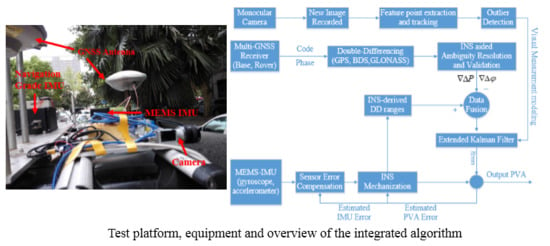
2.5. Overview of the Tightly Integrated Monocular Camera/INS/RTK System

According to the description above, an overview of the proposed tightly coupled monocular camera/INS/RTK integration is shown in Figure 1. After the initialization of the integrated system, the INS mechanization begins to provide high-rate navigation output including the position, velocity, and attitude (PVA). Once the raw GNSS observations from base and rover receivers are available, the DD code and phase observations will be formed. Then, the DD float ambiguities and their corresponding covariance will be calculated using the least-squares adjustment with the INS-derived position constraint. The LAMBDA method is used for ambiguity resolution, and the validation test is conducted subsequently to determine whether the searched ambiguities should be accepted or not. If the validation test is passed, the ambiguity-fixed phase measurements will be fused with the INS-derived DD ranges to update the integrated filter; otherwise, the code measurements will be used. The main reason that we tend to use code measurements instead of ambiguity-float phase measurements is that the satellite signals are interrupted frequently in GNSS-challenged environments. As a result, the accuracy of the float ambiguity is limited due to the frequent reinitialization.

When a new image is arrived, the error state and covariance of the current IMU pose will be augmented into the integrated filter. The corner features are extracted and feature tracking is performed. For those features whose tracks are complete, the EKF updates are performed using the method presented in Section 2.3.

Finally, the estimated IMU sensor errors using a GNSS update or visual update are fed back to compensate for the error of raw IMU data. Meanwhile, the navigation solution provided by INS mechanization is corrected with the estimated errors from the integration filter.

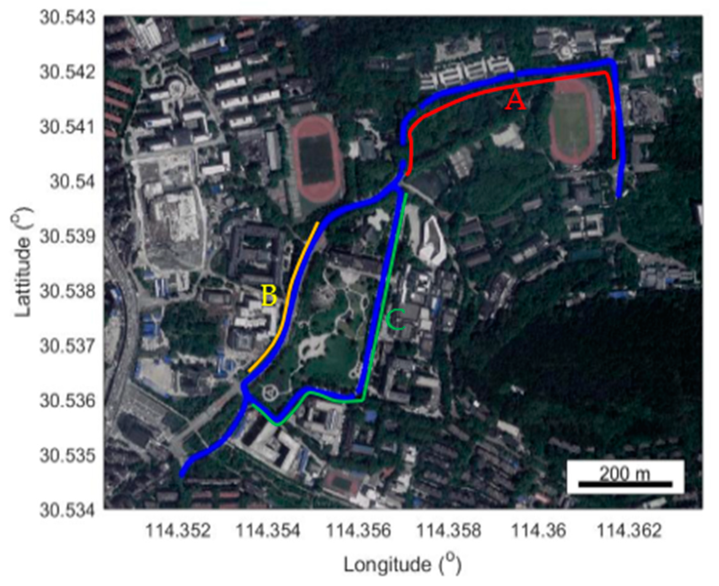
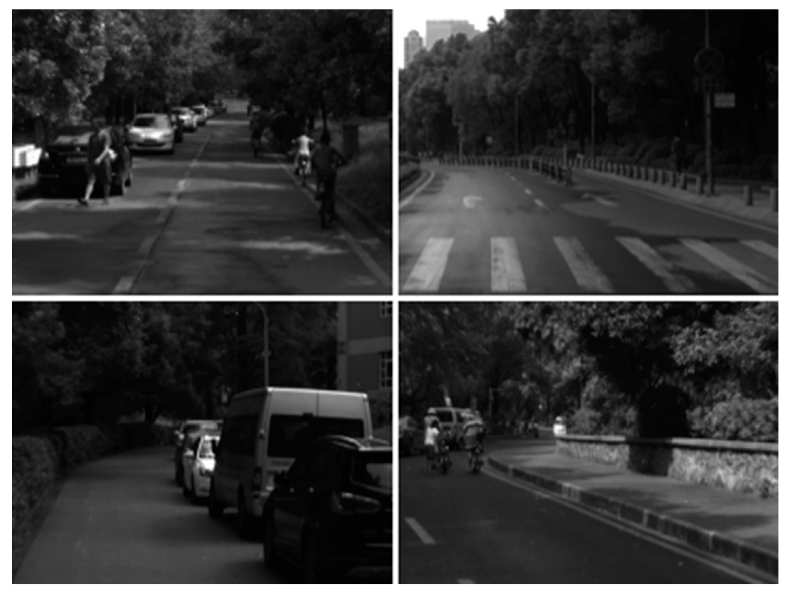
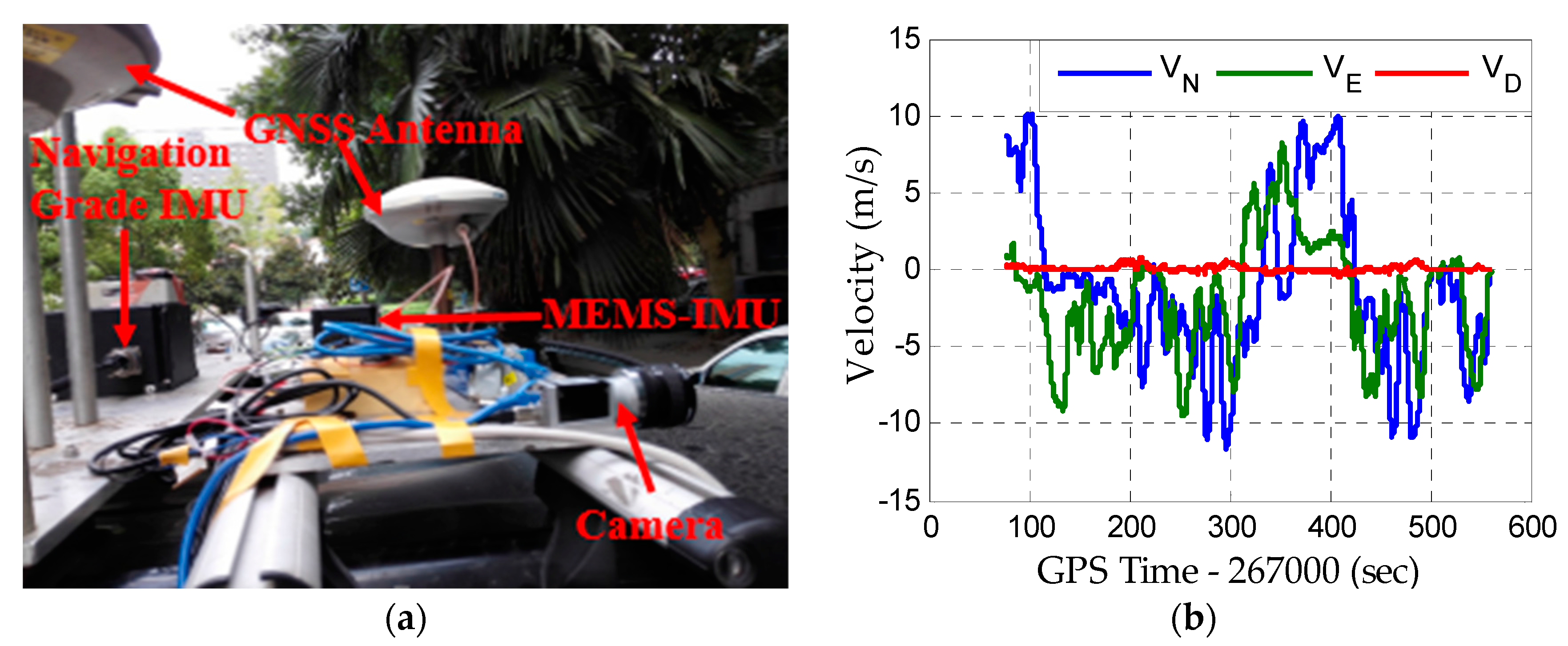
3. Field Test Description and Data Processing Strategy

In order to evaluate the performance of the proposed tightly integrated single-frequency multi-GNSS RTK/INS/Vision algorithm in GNSS-challenged environments, a field vehicular test was carried out at Wuhan University on 15 August 2018. The test trajectory is shown in Figure 2, and several typical scenarios are shown in Figure 3. The test route is mainly on the tree-lined roads, which can be characterized by three different sections as shown in Figure 2. Section A of the route is the most challenged, with tall trees and buildings on the side of the narrow road. Section B of the route is relatively open as the roads are wide and the heights of trees are generally below 3 m. In Section C of the route, the roads are very narrow and only those satellites with high elevation can be tracked continuously by the receiver. This kind of environment poses challenges to the high-precision GNSS positioning due to the frequent signal blockages and multipath.

The test platform and equipment used in this research are shown in Figure 4a. Two different grades of IMUs were used to collect the raw IMU data and their main performance specifications are shown in

Table 1. Performance specifications of the IMU sensors in the experiment.

IMU Sensors	Bias		Random Walk
	$\mathbf{Gyro}.({}^{⚬}/\mathbf{h})$	Acce. (mGal)	$\mathbf{Angular}({}^{⚬}/\sqrt{\mathbf{h}})$	$\mathbf{Velocity}(\mathbf{m}/\mathbf{s}/\sqrt{\mathbf{h}})$
Navigation grade	0.027	15	0.003	0.03
MEMS grade	10.0	1500	0.33	0.18

. The raw data from the MEMS-grade IMU was processed and analyzed to demonstrate the performance of the integrated system, while the navigation-grade IMU was used to obtain the reference solution. The sampling rate of both IMUs was 200 Hz. A greyscale Basler acA1600-20gm camera (Ahrensburg, Germany) was equipped to collect the raw images (20 Hz with resolution 640 × 480 pixels). The camera exposure is triggered by the pulses per second (PPS) generated by the GNSS receiver, and an exposure signal sent out by the camera will be received by the GNSS receiver. In this way, the GPS time of the camera exposure can be recorded precisely. The camera, IMU, and GNSS antenna were fixed rigidly on the top of the vehicle as shown in Figure 4a. The lever-arm offset between the IMU center and the GNSS antenna was measured manually. The intrinsic parameters and camera–IMU extrinsic parameters were calibrated offline [41,42].

The reference station was fixed on the rooftop of the Teaching and Experiment Building of Wuhan University. A Trimble NetR9 multi-GNSS multifrequency receiver (Sunnyvale, CA, USA) was used to collect raw GNSS data at 1 Hz. The rover receiver (Trimble OEM Board) was placed on the car and connected to the GNSS antenna. The whole field test took about 18 min, and the initial alignment of INS was performed at the beginning of the test. After that, we started to collect raw images continuously for about 8 min. The velocity during this period is shown in Figure 4b. It can be seen that there are frequent periods of acceleration and that the maximum velocity could reach 10 m/s in the north and east directions.

In the GNSS data processing phase, the DD ionospheric and tropospheric delay were neglected as the baseline length was less than 2 km in this field test. In the ambiguity resolution process, the critical ratio was set to 3.0 for the GPS system and 2.0 for the GPS + BDS or the GPS + BDS + GLONASS systems [16]. As the GNSS observations are susceptible to multipath error in GNSS-challenged environments, the fault detection and exclusion (FDE) strategy proposed in [16] was employed to resist the measurement outliers. In this research, only the single-frequency GPS/BDS/GLONASS data were processed to evaluate the navigation performance of the integrated algorithm. The dual-frequency GPS/BDS/GLONASS data and the navigation-grade IMU were used to generate the reference solution by using the tightly coupled RTK/INS integration mode with backward smoothing. For feature extraction, the image was split into cells with fixed size and the FAST corners were extracted with the highest Shi–Tomasi score in the cell [43,44]. When a new image was recorded, the exiting features were tracked by the KLT algorithm [45]. In addition, the fundamental matrix test with random sample consensus (RANSAC) was performed to remove outliers.

4. Results

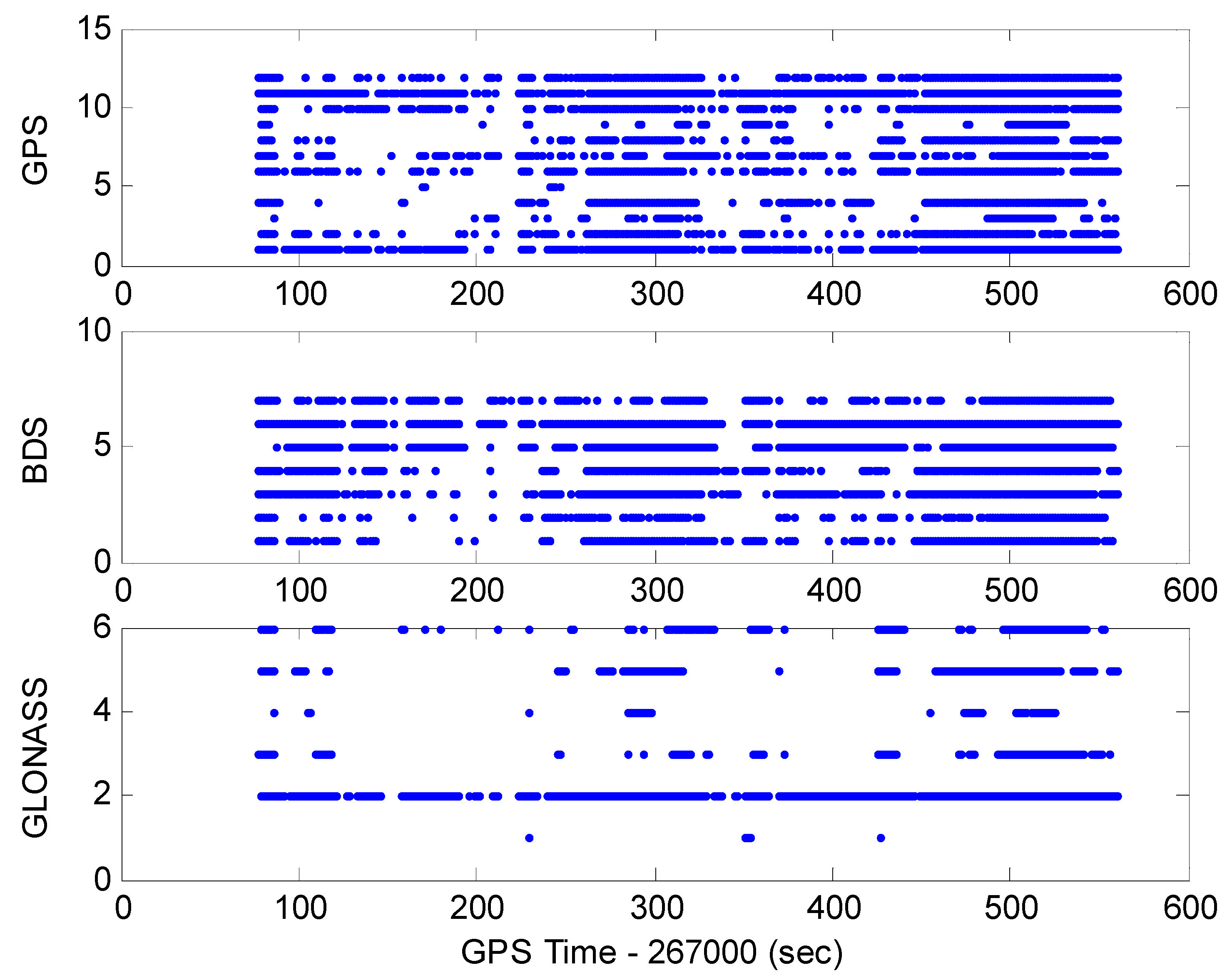
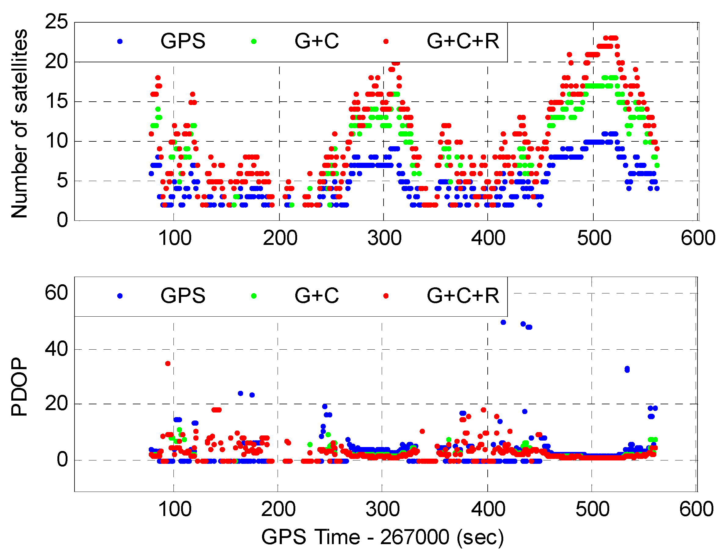
4.1. Satellite Availability

The satellite availability in GNSS-challenged environments is of great importance for high-precision GNSS positioning. Figure 5 shows the satellite visibility of the individual GPS, BeiDou, and GLONASS systems during the field test at a 15° cutoff elevation angle. It can be seen that the satellite signals are interrupted frequently in the tree-lined roads, especially for the GLONASS satellites. The discontinuous tracking condition poses great challenges to GNSS-based positioning.

The number of visible satellites and the corresponding position dilution of precision (PDOP) for the GPS, GPS + BDS (G + C), and GPS + BDS + GLONASS (G + C + R) systems are shown in Figure 6. It indicates that the number of GPS satellites is less than five for most of the time, which means the positioning availability of the GPS-only system is very limited. After the inclusion of the BDS and GLONASS, the number of satellites for positioning is increased significantly and the corresponding average PDOP values of the GPS, GPS + BDS, and GPS + BDS + GLONASS are 10.5, 4.5, and 4.2, respectively. Obviously, the PDOP improvement from the multi-GNSS exceeds 50% in comparison with the GPS-only system.

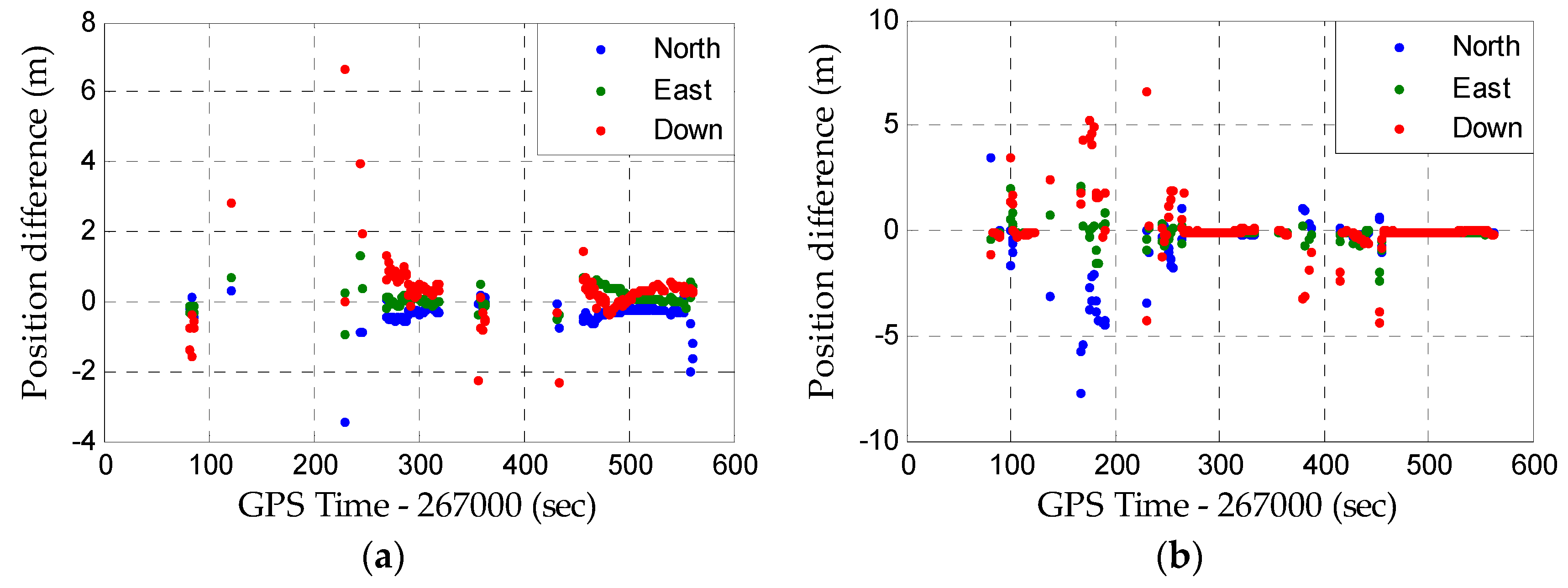
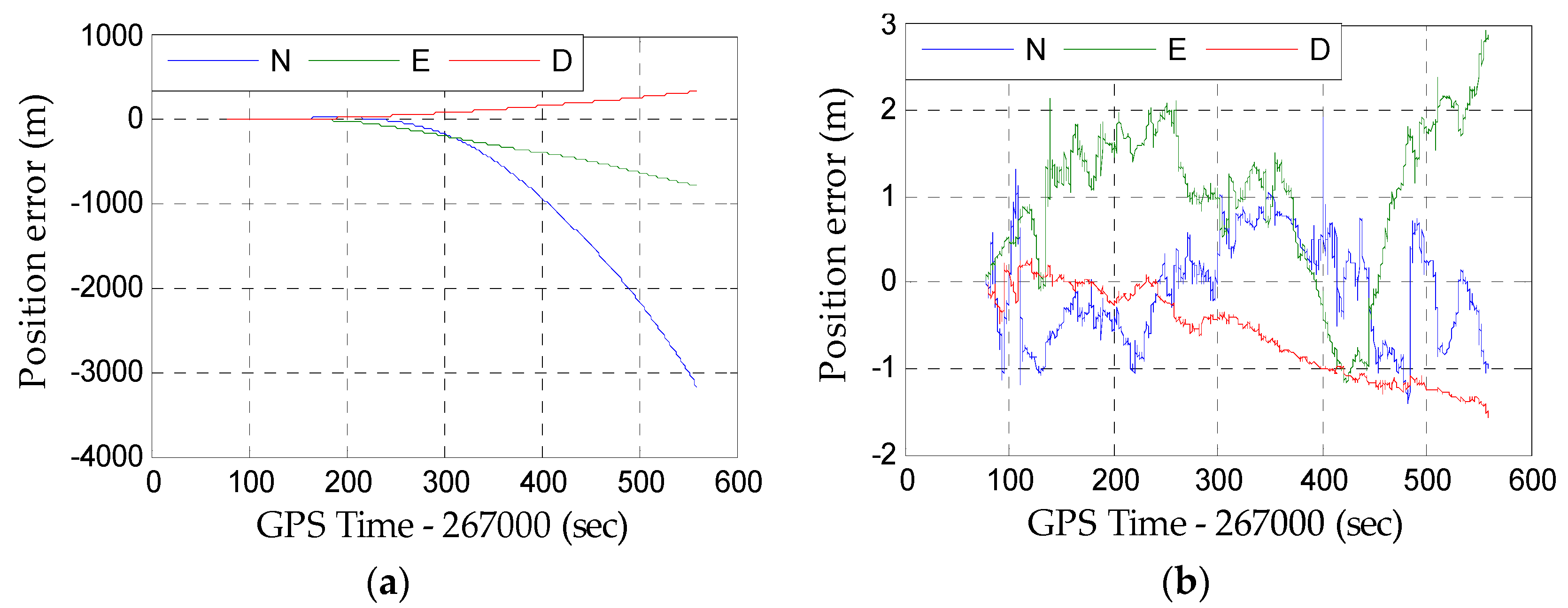
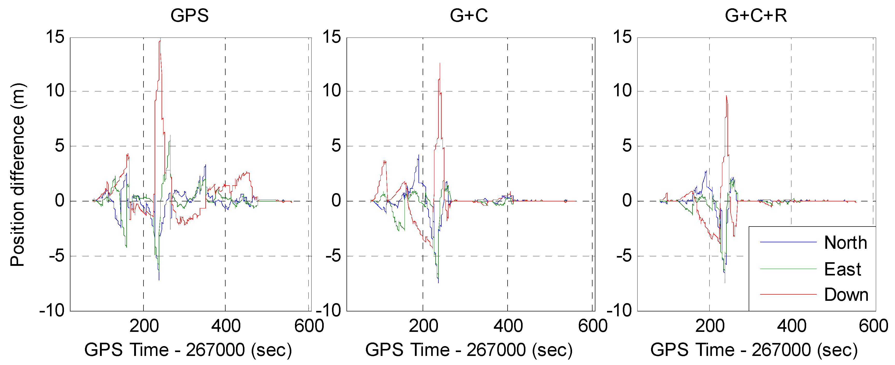
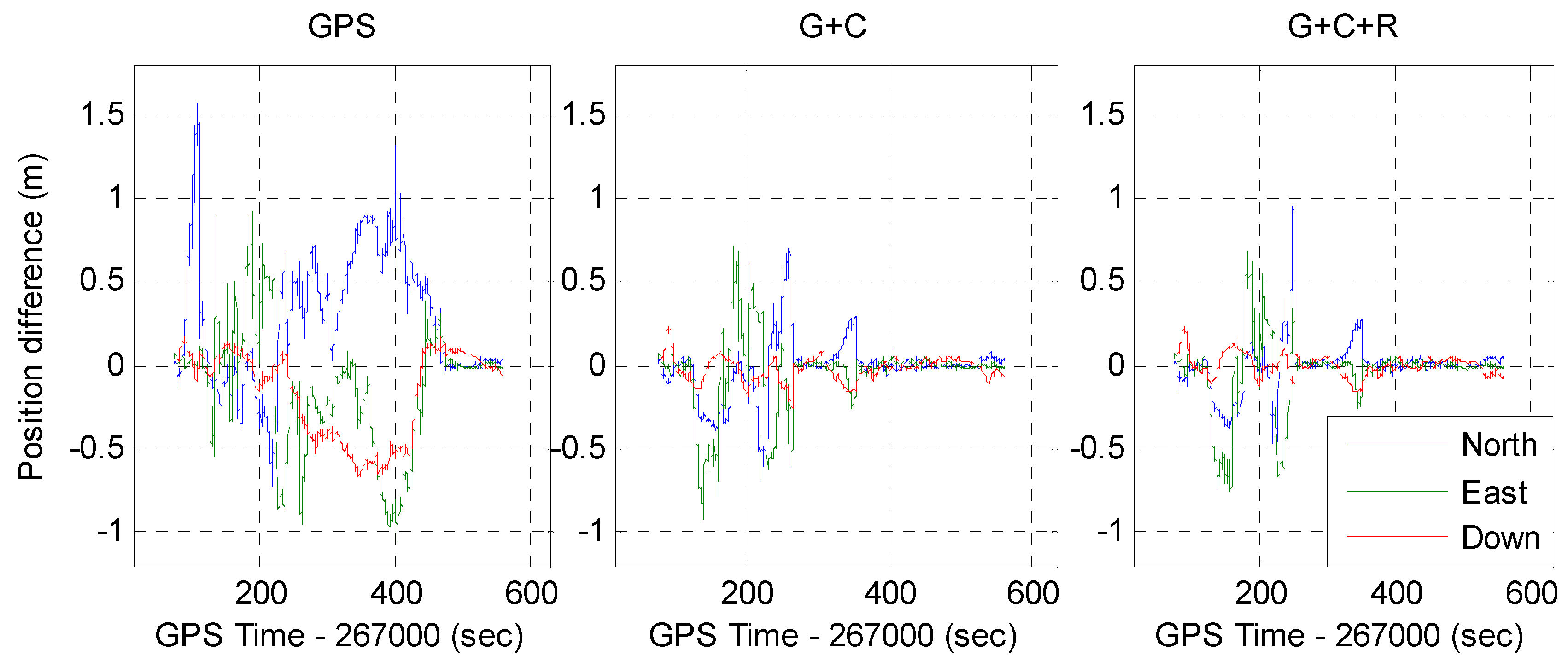
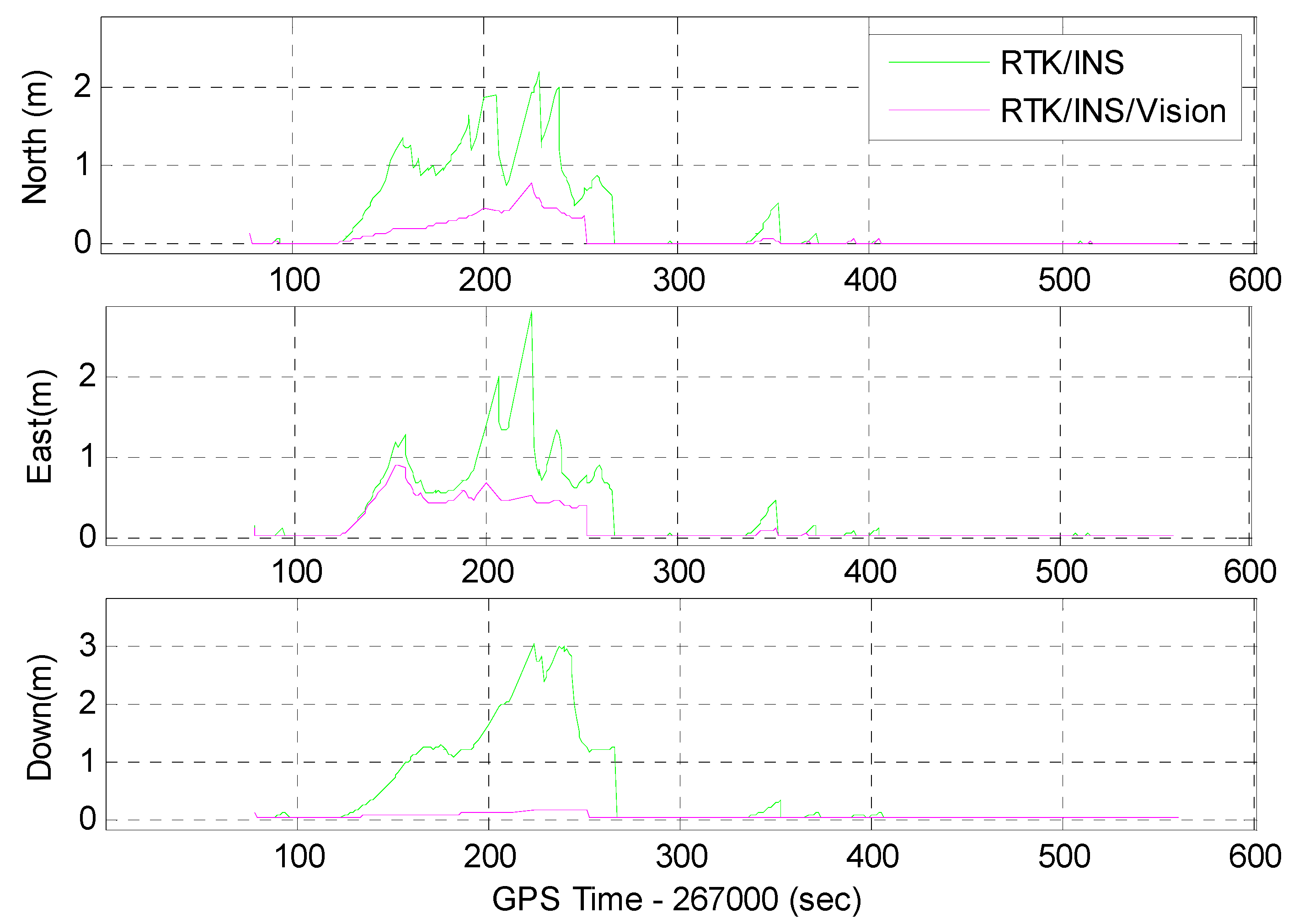
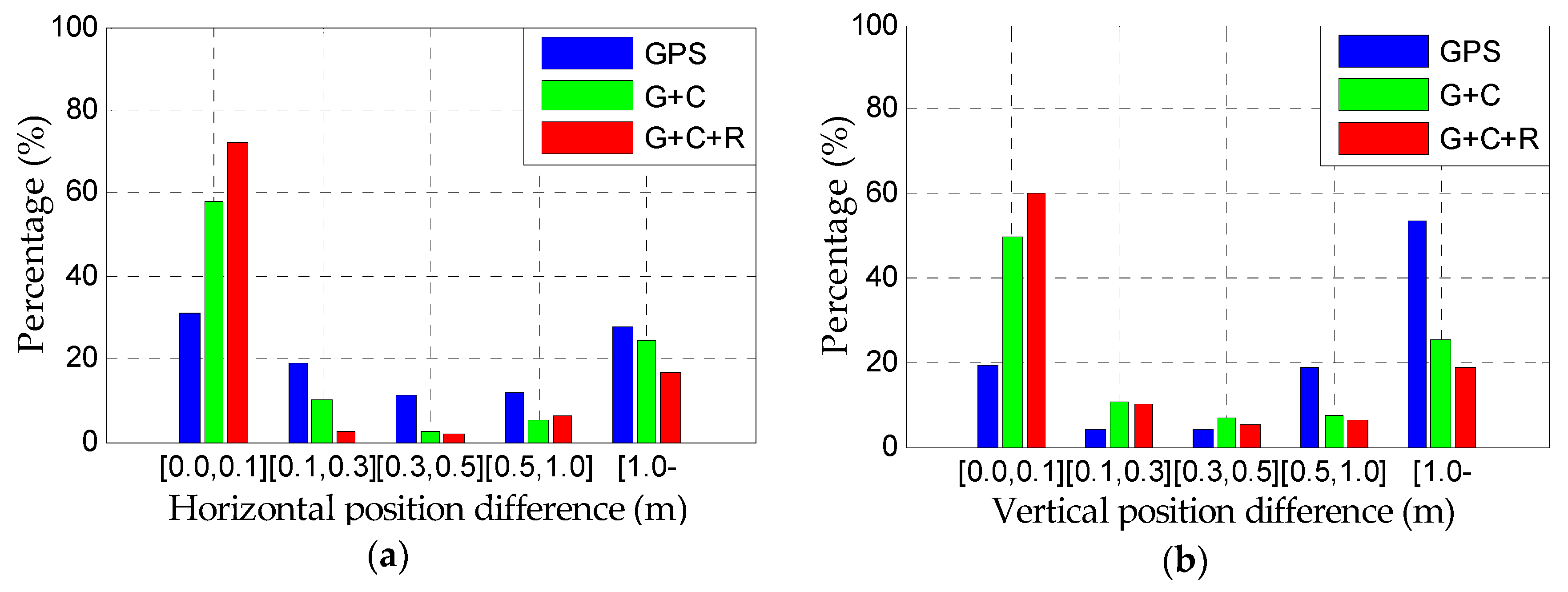
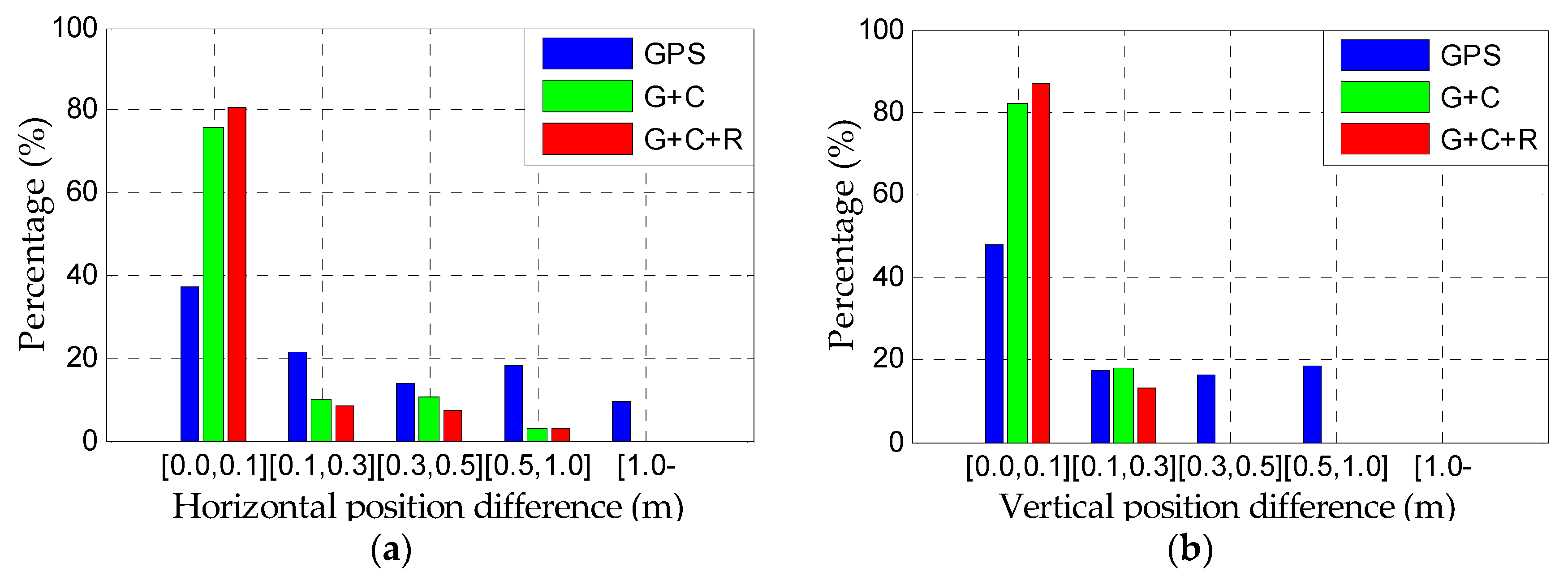
4.2. Positioning Performance

Before showing the benefits of the integrated system in GNSS-challenged environments, the single-frequency RTK positioning results are presented. Figure 7a and b shows the positioning differences of the GPS and GPS + BDS single-frequency RTK with respect to the reference values, respectively. The single-frequency RTK results were calculated using the well-known commercial software GrafNav 8.7 (Calgary, AB, Canada). As the performance of the GPS + BDS RTK does not show obvious improvement with the addition of GLONASS data, we only show the positioning results of the GPS + BDS RTK. It can be seen that the positioning performance of single-frequency GPS RTK is very poor, with positioning availability of only 34.3%, and the ambiguity-fixed solution is not achievable. After the addition of the BDS, the positioning availability reaches 56.9% with an ambiguity fixing rate of 39.1%. Obviously, there are significant improvements when multi-GNSS data is used, but the availability of high-accuracy GNSS positioning is very limited.

Different from the absolute GNSS positioning, the INS can provide a continuous navigation solution alone after initialization. However, the main drawback of INS is the rapid error drift when no external aiding is applied, as shown in Figure 8a. The position drift error arrives at several thousand meters after 8 minutes’ trajectory. When integrated with the monocular vision, the positioning error of INS is reduced significantly, and the maximum three-dimensional (3D) position error is about 3.5 m, as shown in Figure 8b. Considering that the total travelled distance is larger than 4 km, the estimated position error is smaller than 0.1% of the travelled distance.

Although the tight fusion of visual and inertial data could reduce the rapid position error drift, it still suffers from error accumulation. With the inclusion of the multi-GNSS data, it is expected that the positioning performance of the integrated algorithm in GNSS-challenged environments could be enhanced noticeably. The position differences of the tightly coupled RTK/INS and RTK/INS/Vision integration with respect to the reference for the GPS, GPS + BDS (G + C), and GPS + BDS + GLONASS (G + C + R) systems are shown in Figure 9 and Figure 10, respectively. It can be seen that the positioning performance of the tightly coupled RTK/INS/Vision integration has significant improvement in comparison with the tightly coupled RTK/INS integration.

In order to further confirm the obtained results, the covariance analysis was conducted. Figure 11 shows the standard deviation (STD) time series of the GPS + BDS + GLONASS RTK/INS integration and the corresponding RTK/INS/Vision integration in the north, east, and down directions. We can see that the STDs of the RTK/INS/Vision integration are much smaller than that of the RTK/INS integration when the satellite availability is limited. The results also indicate that the accuracy of estimated position has little improvement with visual aiding when enough precise phase measurements are used for filter updates. In addition, the fact that the position errors are contained within 3 STDs confirms the accuracy of the obtained results.

The statistics in terms of the root mean square (RMS) of the position differences of the tightly coupled integration for the three different system configurations is shown in

Table 2. Root mean square (RMS) of the position differences of the tightly coupled RTK/INS and RTK/INS/Vision integration with respect to the reference for the GPS, GPS + BDS (G + C), and GPS + BDS + GLONASS (G + C + R) systems.

	RTK/INS			RTK/INS/Vision			Improvement (%)
RMS(m)	North	East	Down	North	East	Down	North	East	Down
GPS	1.182	1.346	2.717	0.474	0.390	0.308	59.9	71.0	88.7
G + C	1.206	1.097	2.016	0.177	0.232	0.076	85.3	78.9	96.2
G + C + R	1.092	0.985	1.556	0.152	0.219	0.065	86.1	77.8	95.8

. It can be seen that significant improvement is achieved with visual aiding and best performance is obtained by using the tightly coupled GPS + BDS + GLONASS RTK/INS/Vision integration. Compared with the GPS + BDS, the addition of GLONASS only has small improvements. The reason is that the available GLONASS satellite is limited in most time of the test, as shown in Figure 5. Additionally, the position RMS in the down direction shows greater improvement than that of the horizontal directions. This is mainly because the position error of the RTK/INS integration in the down direction is much larger than the horizontal directions during the period from 267,235 s to 267,250 s, as shown in Figure 9.

As the PDOP can be very large in the field test, the positioning error can be large even though the ambiguities are fixed correctly. Besides, the INS can still provide continuous high-accuracy positioning during short GNSS outages, especially with the visual aiding. Therefore, we tend to use the position difference distribution to evaluate the high-accuracy positioning capability of the integrated system instead of the ambiguity fixing rate. The distribution of the position differences of the tightly coupled RTK/INS integration for the GPS, GPS + BDS, and GPS + BDS + GLONASS is shown in Figure 12. The statistics shows that the percentage of the horizontal position differences within 0.1 m is 30.9, 57.9, and 72.4% for the GPS, GPS + BDS, and GPS + BDS + GLONASS, respectively. The corresponding figures are 19.4, 49.5, and 60.3% for the vertical position differences. It indicates that the vehicle can achieve centimeter-level positioning accuracy over 60% of the time in the field test with the GPS + BDS + GLONASS RTK/INS integration. For the horizontal position differences larger than 1.0 m, the percentage decreases from 27.5% of the GPS RTK/INS integration to 24.2% and 17.0% of the GPS + BDS RTK/INS and GPS + BDS + GLONASS RTK/INS, respectively. The corresponding percentage of the vertical position differences larger than 1.0 m is 53.7, 25.5, and 18.8% for the three different system configurations, respectively. Obviously, there are significant improvements when the multi-GNSS data is used in the RTK/INS integration.

The results of the tightly coupled RTK/INS/Vision integration for the GPS, GPS + BDS and GPS + BDS + GLONASS are shown in Figure 13. As expected, the RTK/INS/Vision integrated solutions are further improved in comparison with the ones of the RTK/INS shown in Figure 12. The statistics indicates that the percentage of the horizontal position differences within 0.1 m is 37.0, 76.0, and 80.9%, with improvements of 6.1, 18.1, and 8.5% for the GPS, GPS + BDS, and GPS + BDS + GLONASS, respectively. The corresponding improvements for the vertical position differences within 0.1 m is 28.4, 32.4, and 26.5% for the GPS, GPS + BDS, and GPS + BDS + GLONASS, respectively. The results also indicate that the percentage of the centimeter-level positioning reaches 80% and decimeter-level positioning accuracy is achieved during the whole field test with the tightly coupled multi-GNSS RTK/INS/Vision integration.

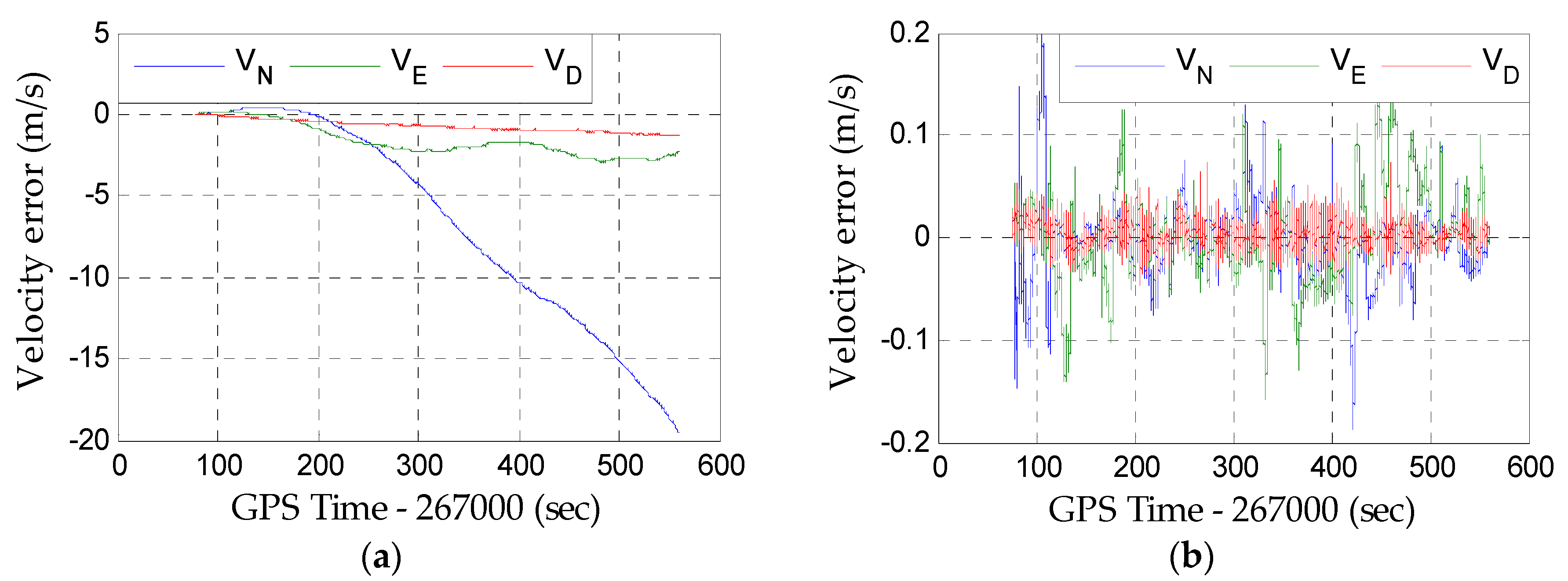
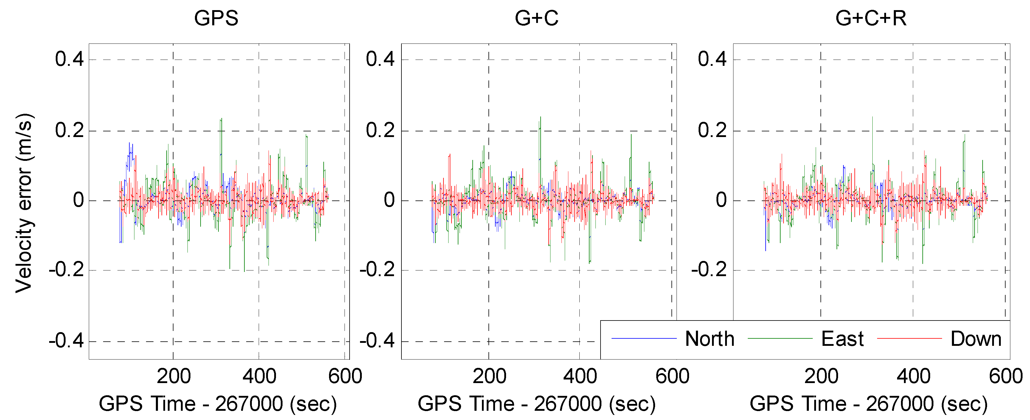
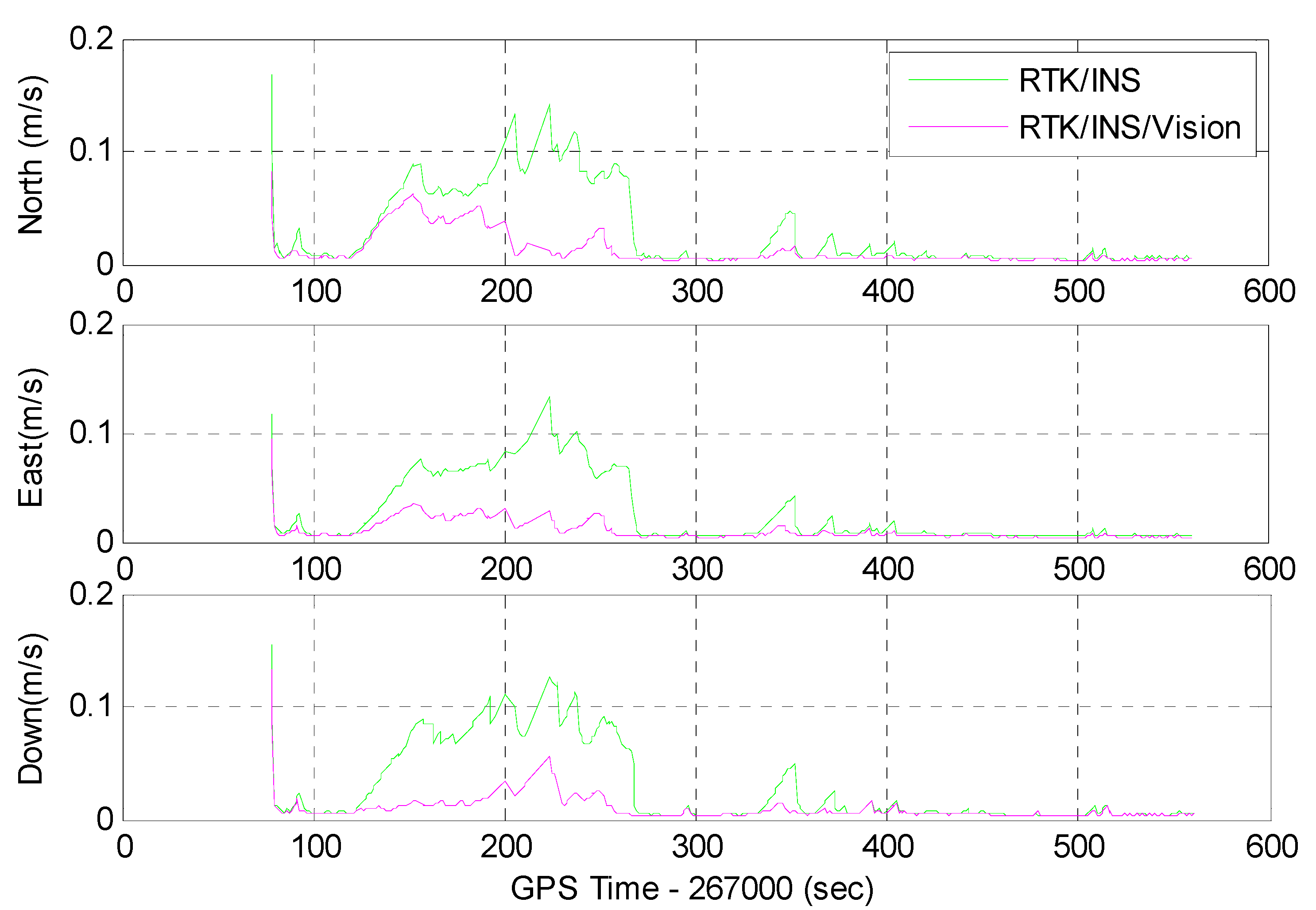
4.3. Velocity Performance

For vehicular navigation, the velocity is another crucial parameter. Therefore, it is necessary to analyze the velocity accuracy of the integrated algorithm in GNSS-challenged environments. We first compare the velocity error of the INS-only and the vision-aided INS solution in Figure 14. It shows that the velocity errors of INS are increased greatly without external aid. The statistics indicates that the velocity error of INS arrives at −19.539, −2.310, and −1.339 m/s in the north, east, and down directions, respectively. By contrast, the velocity error is bounded with the visual aids as the velocity of the visual–inertial system is observable.

The time series of the velocity error of the tightly coupled RTK/INS and RTK/INS/Vision integration for the GPS, GPS + BDS, and GPS + BDS + GLONASS are shown in Figure 15 and Figure 16, respectively. It can be seen that the velocity error of the tightly coupled RTK/INS integration increases slightly during short GNSS outages. After the inclusion of visual data, the velocity error is within 0.2 m/s in the north, east, and down directions for all three system configurations. Figure 17 shows the velocity STD series of the GPS + BDS + GLONASS RTK/INS integration and the corresponding RTK/INS/Vision integration in the north, east, and down directions. It indicates that the velocity accuracy can be greatly improved with visual aiding when the GNSS performance is degraded, and both precise GNSS and visual measurements contribute to the velocity estimation.

According to the statistics in

Table 3. RMS of the velocity error of the tightly coupled RTK/INS and RTK/INS/Vision integration for the GPS, GPS + BDS (G+C), and GPS + BDS + GLONASS (G+C+R).

	RTK/INS			RTK/INS/Vision			Improvement (%)
RMS (m/s)	North	East	Down	North	East	Down	North	East	Down
GPS	0.092	0.119	0.075	0.038	0.050	0.025	58.7	58.0	66.7
G+C	0.091	0.103	0.075	0.028	0.048	0.025	69.2	53.4	66.7
G+C+R	0.082	0.094	0.055	0.028	0.046	0.025	65.9	51.1	54.5

, the velocity RMS values of the tightly coupled GPS RTK/INS integration are 0.092, 0.119, and 0.075 m/s in the north, east, and down directions, respectively. Comparatively, the velocity accuracy shows little improvement for the GPS + BDS and GPS + BDS + GLONASS system. The main reason is that the velocity drift error is small during short GNSS outages, and its accuracy is mainly dependent on the IMU performance [46]. Compared with the velocity of the tightly coupled RTK/INS integration, the velocity accuracy of the tightly coupled RTK/INS/Vision integration is much better. The statistics indicates that the average velocity RMSs of the three different RTK/INS/Vision integrations are about 0.031, 0.048, and 0.025 m/s in the north, east, and down directions, respectively. Compared to that of the tightly coupled RTK/INS integration, the average improvements are about 64.5, 54.4, and 63.4% in the north, east, and down directions, respectively.

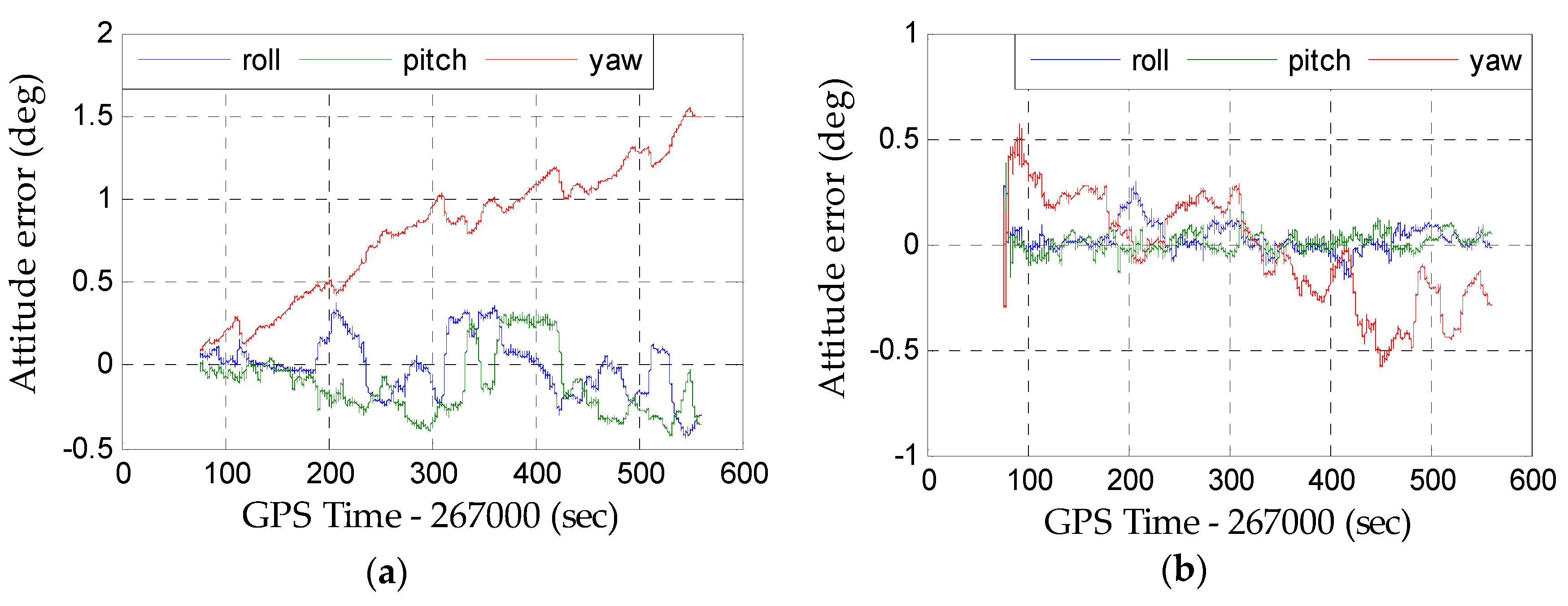
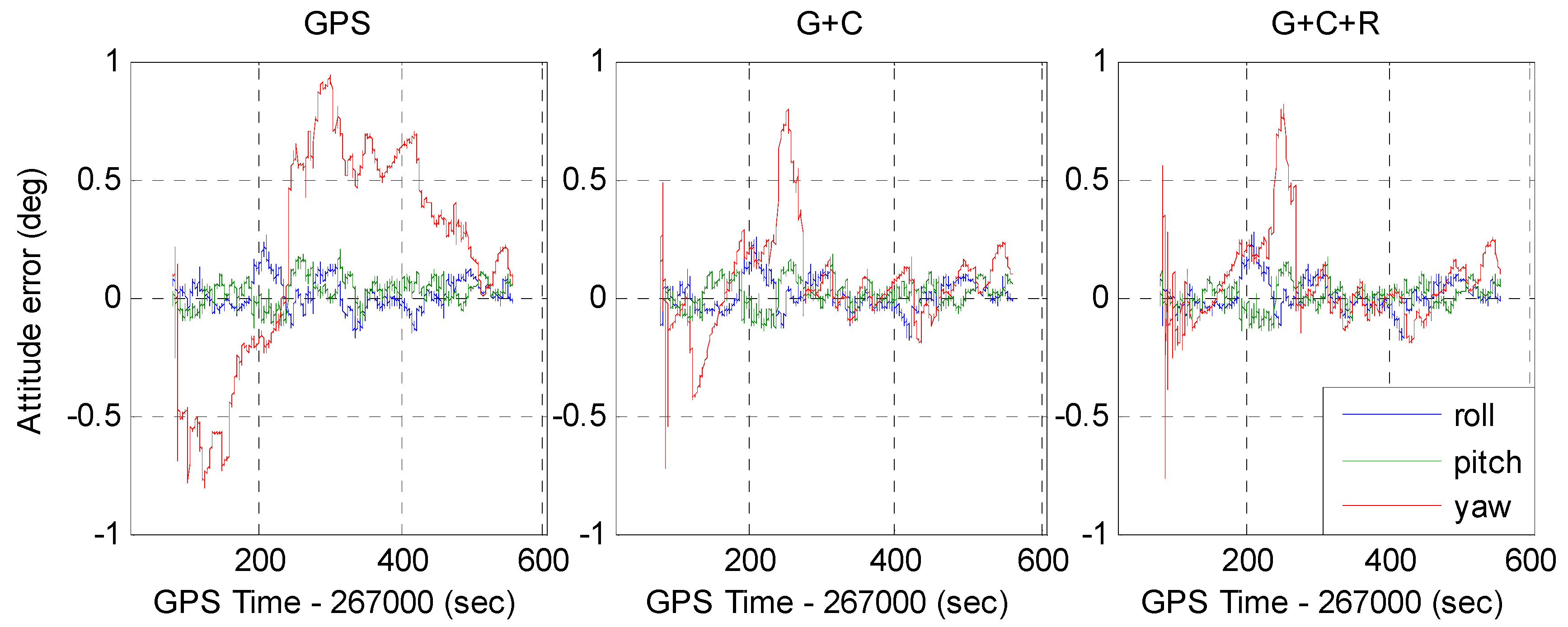
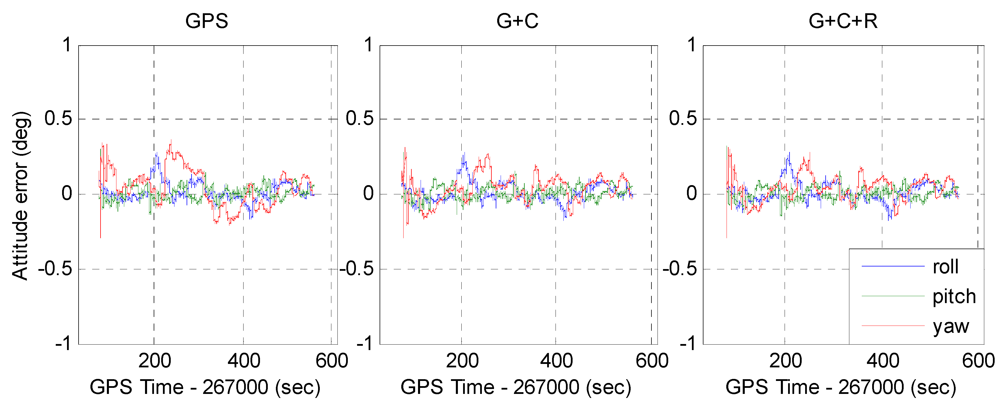
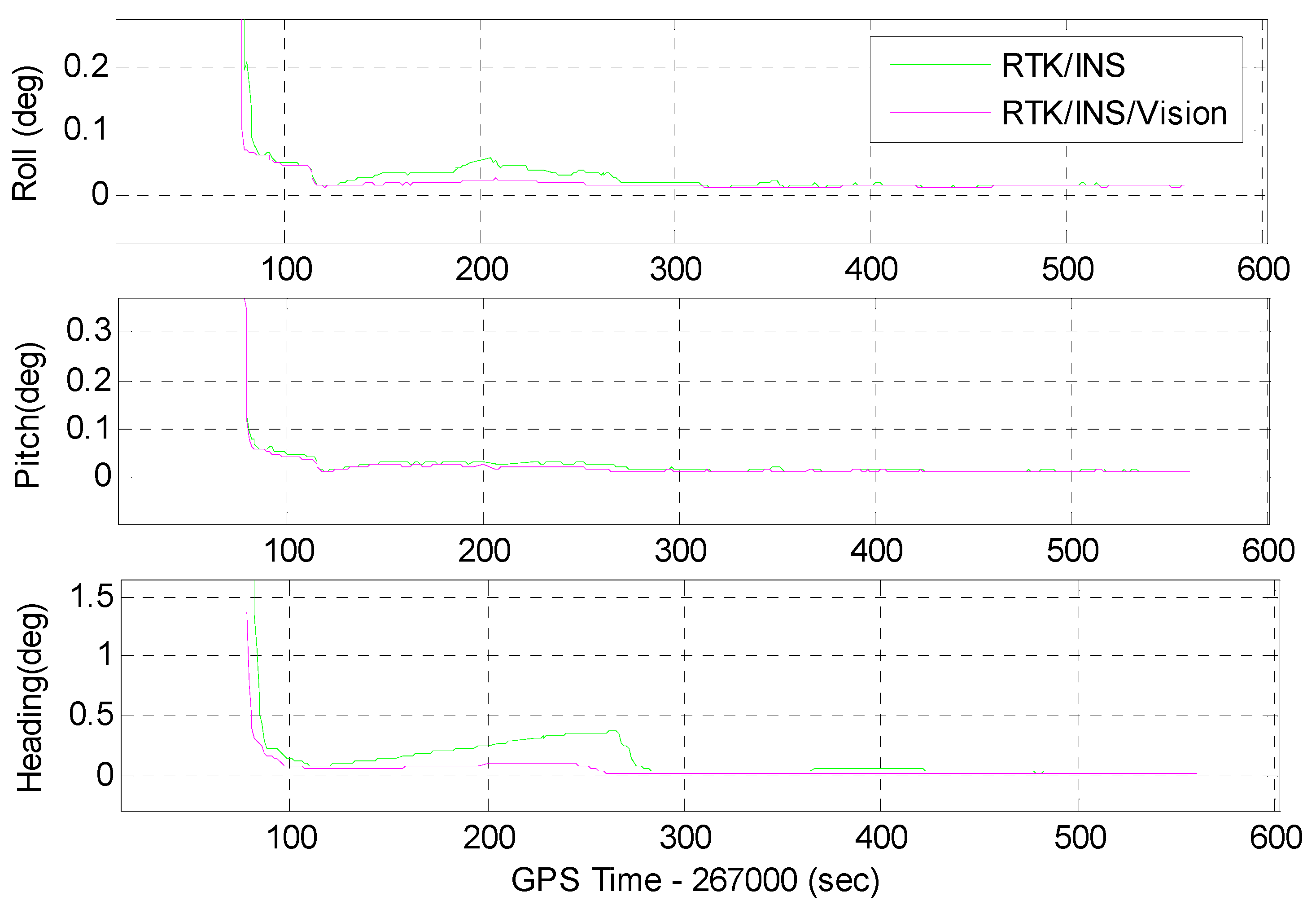
4.4. Attitude Performance

Similar to the position and velocity, the attitude accuracy is also necessary for applications such as machine control and mobile mapping. Although the INS can provide high-accuracy attitude for the vehicle, the attitude error suffers from drifts, especially for the yaw angle while using the low-cost MEMS-IMU. Figure 18a shows the attitude error of the INS-only solution during the field test. It indicates that the yaw error increases more rapidly than that of the roll and pitch angles. When integrated with the visual data, the speed of the yaw error drift becomes lower, as shown in Figure 18b, even though the yaw error still accumulates due to the unobservability of yaw angle in the visual–inertial system. The results also show that the errors of roll and pitch angles are bounded without any drift. This is because the roll and pitch angles and the IMU gyroscope bias can be recovered from the monocular camera and IMU measurements alone [47]. With the estimated gyroscope bias, the drift speed of attitude will become slower [48].

The time series of the attitude error of the tightly coupled RTK/INS and RTK/INS/Vision integration for the GPS, GPS + BDS, and GPS + BDS + GLONASS are shown in Figure 19 and Figure 20, respectively. It can be seen that the roll, pitch, and yaw angles are all observable, and the accuracy of yaw angle can be improved significantly with visual aiding. The series of attitude STDs shown in Figure 21 also indicates that the yaw error drift more rapidly than the roll and pitch error, and the drift speed of yaw angle is much slower with visual aiding. The corresponding statistics in terms of the RMS of the attitude error is shown in

Table 4. RMS of the attitude error of the tightly coupled RTK/INS and RTK/INS/Vision integration for the GPS, GPS + BDS (G+C), and GPS + BDS + GLONASS (G+C+R).

	RTK/INS			RTK/INS/Vision			Improvement (%)
RMS (deg)	Roll	Pitch	Yaw	Roll	Pitch	Yaw	Yaw
GPS	0.070	0.063	0.500	0.066	0.046	0.134	73.2
G + C	0.066	0.058	0.214	0.065	0.045	0.099	53.7
G + C + R	0.068	0.052	0.198	0.066	0.044	0.092	53.5

.

The statistics in Table 4 shows that the RMSs of roll and pitch error are about 0.04–0.07° for both the tightly coupled RTK/INS and RTK/INS/Vision integration in three different system configurations. The reason why they show little difference is that the error drifts of roll and pitch angles are very small during short GNSS outages, and they can be recovered once the GNSS positioning is available. By contrast, the accuracy of yaw angle can be improved significantly while using the multi-GNSS and visual data. Generally, the observability and achievable accuracy of the yaw angle is worse than that of the roll and pitch angle in the GNSS/INS integration. If no effective GNSS measurements are used for the filter update, the yaw angle drifts rapidly. Significantly, both the multi-GNSS and vision bring benefits to the yaw angle accuracy. The improved accuracy of yaw angle is of great importance for those attitude-critical applications.

5. Discussion

Precise navigation in GNSS-constrained areas is still very challenging, especially in the position component. According to the presented results, the centimeter-level positioning availability can be increased significantly by using the tightly coupled multi-GNSS RTK/INS/Vision integration in GNSS-challenged environments. The percentage of the centimeter-level positioning is increased from about 30% of the GPS RTK/INS integration to about 60% of the GPS + BDS + GLONASS RTK/INS integration. After the inclusion of vision, the corresponding percentages are about 37% and 80% for the GPS and GPS + BDS + GLONASS RTK/INS/Vision integration, respectively. The main reason behind this is that the ambiguity resolution performance of single-frequency RTK can be improved greatly by using the multi-GNSS [4,6,7,8,16]. According to some previous research in the robotics community, the position error of the MEMS-IMU can be greatly reduced when integrated with vision [17,18,19,20,21,22,23]. The comparable accuracy was also obtained with position error smaller than 0.1% of the travelled distance in our experiments.

In terms of the attitude accuracy, the significant improvement is obtained for the yaw angle by using the RTK/INS/Vision integration. Although the yaw angle of the visual–inertial system is not observable, the gyroscope bias can be recovered [47]. As a result, the yaw angle drifts slowly with time and its accuracy is improved (Table 4). For the low-cost GNSS/MEMS-IMU integration, the yaw angle drifts rapidly during GNSS outages. It is meaningful that the visual aiding information can restrict the rapid error growth of yaw angle greatly.

We also notice that the position accuracy of the GPS + BDS + GLONASS RTK/INS/Vision integration is a little worse than that of the GPS + BDS RTK/INS/Vision integration around epoch 267, 240 s (Figure 10). It may be caused by the unmodeled pseudorange errors from the GLONASS satellites. As shown in Figure 6, the available satellites are very limited during that time, and it will be difficult to model the errors properly when the position error of the integrated system is large. Therefore, further efforts are still needed to deal with this kind of situation.

6. Conclusions

The demand for precise navigation has been increased dramatically with the development of unmanned vehicles. In this contribution, we introduced the tightly coupled single-frequency multi-GNSS RTK/INS/Vision integration model and validated it by using a field vehicular test in GNSS-challenged environments. The navigation performance in terms of the position, velocity, and attitude were evaluated. According to the results, the conclusions can be drawn as follows.

The RTK positioning performance is markedly degraded in GNSS-constrained environments; therefore, the high-accuracy RTK positioning with high availability is not possible even with the multi-GNSS. The positioning performance in terms of the accuracy, continuity, and availability is improved significantly with the tightly coupled RTK/INS and RTK/INS/Vision integrations. The experimental results indicate that the position RMS of the tightly coupled GPS + BDS + GLONASS RTK/INS integration is 1.092, 0.985, and 1.556 m in the north, east, and down directions, respectively. The corresponding figure are decreased to 0.152, 0.219, and 0.065 m for the tightly coupled GPS + BDS + GLONASS RTK/INS/Vision integration. The results also indicate that the percentage of the centimeter-level positioning is below 30% and 37% for the GPS RTK/INS integration and the corresponding RTK/INS/Vision integration, respectively. By comparison, the percentages for the multi-GNSS RTK/INS integration and the corresponding RTK/INS/Vision integration are over 60% and 80%, respectively. Obviously, both multi-GNSS and vision bring benefits to the centimeter-level positioning in GNSS-challenged environments.

The results also indicate that the velocity and yaw attitude performance can be greatly improved after the inclusion of visual data, compared with the RTK/INS integration. The average velocity RMSs of the three different RTK/INS/Vision integrations are about 0.031, 0.048, and 0.025 m/s, and the corresponding improvements are about 64.5, 54.4, and 63.4% in the north, east, and down directions, respectively. The RMS of yaw error is decreased from 0.500, 0.214, and 0.198° of the RTK/INS integration to 0.134, 0.099, and 0.092° of the RTK/INS/Vision integration for the GPS, GPS + BDS, and GPS + BDS + GLONASS, respectively.

According to the results, it is still not possible to achieve centimeter-level positioning during long GNSS outages using the low-cost tightly coupled integration of a monocular camera, MEMS-IMU, and single-frequency multi-GNSS RTK. Comparatively, high-accuracy velocity and attitude information can be obtained using the proposed integration algorithm.

Since the feature-based visual measurement model relies on the consecutive tracking of static features, robust feature tracking and outlier-resistant methods should be developed to make the algorithm more practical in complex environments such as urban roads with many cars and pedestrians. In addition, the wheel odometry can be adopted for land vehicle applications to enhance the navigation performance.

References

1. Martin, P.G.; Payton, O.D.; Fardoulis, J.S.; Richards, D.A.; Scott, T.B. The use of unmanned aerial systems for the mapping of legacy uranium mines. J. Environ. Radioact. 2015, 143, 135–140. [Google Scholar] [CrossRef] [PubMed] [Green Version]
2. Albéri, M.; Baldoncini, M.; Bottardi, C.; Chiarelli, E.; Fiorentini, G.; Raptis, K.G.C.; Realini, E.; Reguzzoni, M.; Rossi, L.; Sampietro, D.; et al. Accuracy of Flight Altitude Measured with Low-Cost GNSS, Radar and Barometer Sensors: Implications for Airborne Radiometric Surveys. Sensors 2017, 17, 1889. [Google Scholar] [CrossRef] [PubMed]
3. Leick, A.; Rapoport, L.; Tatarnikov, D. GPS Satellite Surveying; John Wiley & Sons: Hoboken, NJ, USA, 2015. [Google Scholar]
4. He, H.; Li, J.; Yang, Y.; Xu, J.; Guo, H.; Wang, A. Performance assessment of single- and dual-frequency BeiDou/GPS single-epoch kinematic positioning. GPS Solut. 2014, 18, 393–403. [Google Scholar] [CrossRef]
5. Carcanague, S.; Julien, O.; Vigneau, W.; Macabiau, C. Low-cost Single-frequency GPS/GLONASS RTK for Road Users. In Proceedings of the ION 2013 Pacific PNT Meeting, Honolulu, HI, USA, 23–25 April 2013; pp. 168–184. [Google Scholar]
6. Teunissen, P.J.G.; Odolinski, R.; Odijk, D. Instantaneous BeiDou+GPS RTK positioning with high cut-off elevation angles. J. Geod. 2013, 88, 335–350. [Google Scholar] [CrossRef]
7. Odolinski, R.; Teunissen, P.J.G. Low-cost, high-precision, single-frequency GPS–BDS RTK positioning. GPS Solut. 2017, 21, 1315–1330. [Google Scholar] [CrossRef]
8. Odolinski, R.; Teunissen, P.J.G.; Odijk, D. Combined BDS, Galileo, QZSS and GPS single-frequency RTK. GPS Solut. 2014, 19, 151–163. [Google Scholar] [CrossRef]
9. Li, T.; Zhang, H.; Niu, X.; Gao, Z. Tightly-Coupled Integration of Multi-GNSS Single-Frequency RTK and MEMS-IMU for Enhanced Positioning Performance. Sensors 2017, 17, 2462. [Google Scholar] [CrossRef] [PubMed]
10. Grejner-Brzezinska, D.A.; Da, R.; Toth, C. GPS error modeling and OTF ambiguity resolution for high-accuracy GPS/INS integrated system. J. Geod. 1998, 72, 626–638. [Google Scholar] [CrossRef]
11. Niu, X.; Zhang, Q.; Gong, L.; Liu, C.; Zhang, H.; Shi, C.; Wang, J.; Coleman, M. Development and evaluation of GNSS/INS data processing software for position and orientation systems. Surv. Rev. 2015, 47, 87–98. [Google Scholar] [CrossRef]
12. Gao, Z.; Ge, M.; Shen, W.; Zhang, H.; Niu, X. Ionospheric and receiver DCB-constrained multi-GNSS single-frequency PPP integrated with MEMS inertial measurements. J. Geod. 2017, 91, 1351–1366. [Google Scholar] [CrossRef]
13. Chiang, K.-W.; Duong, T.; Liao, J.-K. The Performance Analysis of a Real-Time Integrated INS/GPS Vehicle Navigation System with Abnormal GPS Measurement Elimination. Sensors 2013, 13, 10599. [Google Scholar] [CrossRef] [PubMed]
14. Falco, G.; Gutiérrez, C.C.; Serna, E.P.; Zacchello, F.; Bories, S. Low-cost Real-time Tightly-Coupled GNSS/INS Navigation System Based on Carrier-phase Double- differences for UAV Applications. In Proceedings of the 27th International Technical Meeting of the Satellite Division of The Institute of Navigation (ION GNSS 2014), Tampa, FL, USA, 8–12 September 2014; pp. 841–857. [Google Scholar]
15. Eling, C.; Klingbeil, L.; Kuhlmann, H. Real-Time Single-Frequency GPS/MEMS-IMU Attitude Determination of Lightweight UAVs. Sensors 2015, 15, 26212. [Google Scholar] [CrossRef] [PubMed]
16. Li, T.; Zhang, H.; Gao, Z.; Chen, Q.; Niu, X. High-accuracy positioning in urban environments using single-frequency multi-GNSS RTK/MEMS-IMU integration. Remote Sens. 2018, 10, 205. [Google Scholar] [CrossRef]
17. Mourikis, A.I.; Roumeliotis, S.I. A multi-state constraint Kalman filter for vision-aided inertial navigation. In Proceedings of the IEEE International Conference on Robotics and Automation, Roma, Italy, 10–14 April 2007; pp. 3565–3572. [Google Scholar]
18. Li, M.; Mourikis, A.I. High-precision, consistent EKF-based visual-inertial odometry. Int. J. Robot. Res. 2013, 32, 690–711. [Google Scholar] [CrossRef]
19. Bloesch, M.; Omari, S.; Hutter, M.; Siegwart, R. Robust visual inertial odometry using a direct EKF-based approach. In Proceedings of the IEEE/RSJ International Conference on Intelligent Robots and Systems, Hamburg, Germany, 28 September–2 October 2015; pp. 298–304. [Google Scholar]
20. Wu, K.; Ahmed, A.; Georgiou, G.; Roumeliotis, S. A Square Root Inverse Filter for Efficient Vision-aided Inertial Navigation on Mobile Devices. In Proceedings of the Robotics: Science and Systems, Rome, Italy, 13–17 July 2015. [Google Scholar]
21. Leutenegger, S.; Lynen, S.; Bosse, M.; Siegwart, R.; Furgale, P. Keyframe-based visual–inertial odometry using nonlinear optimization. Int. J. Robot. Res. 2015, 34, 314–334. [Google Scholar] [CrossRef]
22. Mur-Artal, R.; Tardos, J.D. Visual-Inertial Monocular SLAM with Map Reuse. IEEE Robot. Autom. Lett. 2016, 2, 796–803. [Google Scholar] [CrossRef]
23. Qin, T.; Li, P.; Shen, S. VINS-Mono: A Robust and Versatile Monocular Visual-Inertial State Estimator. IEEE Trans. Robot. 2018, 34, 1004–1020. [Google Scholar] [CrossRef]
24. Grejner-Brzezinska, D.A.; Toth, C.K.; Moore, T.; Raquet, J.F.; Miller, M.M.; Kealy, A. Multisensor Navigation Systems: A Remedy for GNSS Vulnerabilities? Proc. IEEE 2016, 104, 1339–1353. [Google Scholar] [CrossRef] [Green Version]
25. Kim, J.; Sukkarieh, S. SLAM aided GPS/INS navigation in GPS denied and unknown environments. Positioning 2005, 4, 120–128. [Google Scholar] [CrossRef]
26. Wang, J.; Garratt, M.; Lambert, A.; Wang, J.J.; Han, S.; Sinclair, D. Integration of GPS/INS/vision sensors to navigate unmanned aerial vehicles. In Proceedings of the International Society of Photogrammetry and Remote Sensing (ISPRS) Congress, Beijing, China, 3–11 July 2008; pp. 963–970. [Google Scholar]
27. Chu, T.; Guo, N.; Backén, S.; Akos, D. Monocular camera/IMU/GNSS integration for ground vehicle navigation in challenging GNSS environments. Sensors 2012, 12, 3162–3185. [Google Scholar] [CrossRef] [PubMed]
28. Oskiper, T.; Samarasekera, S.; Kumar, R. Multi-sensor navigation algorithm using monocular camera, IMU and GPS for large scale augmented reality. In Proceedings of the IEEE International Symposium on Mixed and Augmented Reality (ISMAR), Atlanta, GA, USA, 5–8 November 2012; pp. 71–80. [Google Scholar]
29. Vu, A.; Ramanandan, A.; Chen, A.; Farrell, J.A.; Barth, M. Real-Time Computer Vision/DGPS-Aided Inertial Navigation System for Lane-Level Vehicle Navigation. IEEE Trans. Intell. Transp. Syst. 2012, 13, 899–913. [Google Scholar] [CrossRef]
30. Lynen, S.; Achtelik, M.W.; Weiss, S.; Chli, M.; Siegwart, R. A robust and modular multi-sensor fusion approach applied to mav navigation. In Proceedings of the IEEE/RSJ International Conference on Intelligent Robots and Systems, Tokyo, Japan, 3–7 November 2013; pp. 3923–3929. [Google Scholar]
31. Shepard, D.P.; Humphreys, T.E. High-precision globally-referenced position and attitude via a fusion of visual SLAM, carrier-phase-based GPS, and inertial measurements. In Proceedings of the IEEE/ION Position, Location and Navigation Symposium—PLANS 2014, Monterey, CA, USA, 5–8 May 2014; pp. 1309–1328. [Google Scholar]
32. Mascaro, R.; Teixeira, L.; Hinzmann, T.; Siegwart, R.; Chli, M. GOMSF: Graph-Optimization based Multi-Sensor Fusion for robust UAV pose estimation. In Proceedings of the IEEE International Conference on Robotics and Automation (ICRA 2018), Brisbane, Australia, 21–25 May 2018; pp. 1421–1428. [Google Scholar]
33. Jekeli, C. Inertial navigation systems with geodetic applications; Walter de Gruyter: Berlin, Germany, 2012. [Google Scholar]
34. Park, M. Error Analysis and Stochastic Modeling of MEMS Based Inertial Sensors for Land Vehicle Navigation Applications. Ph.D. Thesis, University of Calgary, Calgary, AL, Canada, 2004. [Google Scholar]
35. Wanninger, L. Carrier-phase inter-frequency biases of GLONASS receivers. J. Geod. 2012, 86, 139–148. [Google Scholar] [CrossRef]
36. Tian, Y.; Ge, M.; Neitzel, F. Particle filter-based estimation of inter-frequency phase bias for real-time GLONASS integer ambiguity resolution. J. Geod. 2015, 89, 1145–1158. [Google Scholar] [CrossRef]
37. Petovello, M. GLONASS inter-frequency biases and ambiguity resolution. Inside GNSS 2009, 4, 24–28. [Google Scholar]
38. Teunissen, P.J.G. The least-squares ambiguity decorrelation adjustment: A method for fast GPS integer ambiguity estimation. J. Geod. 1995, 70, 65–82. [Google Scholar] [CrossRef]
39. Ji, S.; Chen, W.; Ding, X.; Chen, Y.; Zhao, C.; Hu, C. Ambiguity validation with combined ratio test and ellipsoidal integer aperture estimator. J. Geod. 2010, 84, 597–604. [Google Scholar] [CrossRef]
40. Verhagen, S. On the Reliability of Integer Ambiguity Resolution. Navigation 2005, 52, 99–110. [Google Scholar] [CrossRef]
41. Bouguet, J.-Y. Camera Calibration Toolbox for MATLAB. Available online: http://www.vision.caltech.edu/bouguetj/calib_doc/index.html (accessed on 16 October 2018).
42. Furgale, P.; Rehder, J.; Siegwart, R. Unified temporal and spatial calibration for multi-sensor systems. In Proceedings of the IEEE/RSJ International Conference on Intelligent Robots and Systems, Tokyo, Japan, 3–7 November 2013; pp. 1280–1286. [Google Scholar]
43. Rosten, E.; Porter, R.; Drummond, T. Faster and Better: A Machine Learning Approach to Corner Detection. IEEE Trans. Pattern Anal. Mach. Intell. 2010, 32, 105–119. [Google Scholar] [CrossRef] [Green Version]
44. Shi, J.; Tomasi, C. Good Features to Track. In Proceedings of the IEEE Conference on Computer Vision and Pattern Recognition, Seattle, WA, USA, 21–23 June 1994; pp. 593–600. [Google Scholar]
45. Lucas, B.D.; Kanade, T. An iterative image registration technique with an application to stereo vision. In Proceedings of the Intenational Joint Conference on Artificial Intelligence, Vancouver, BC, Canada, 24–28 August 1981; pp. 121–130. [Google Scholar]
46. Gao, Z.; Ge, M.; Shen, W.; You, L.; Chen, Q.; Zhang, H.; Niu, X. Evaluation on the impact of IMU grades on BDS+GPS PPP/INS tightly coupled integration. Adv. Space Res. 2017, 60, 1283–1299. [Google Scholar] [CrossRef]
47. Kelly, J.; Sukhatme, G.S. Visual-inertial sensor fusion: Localization, mapping and sensor-to-sensor self-calibration. Int. J. Robot. Res. 2011, 30, 56–79. [Google Scholar] [CrossRef]
48. Sinpyo, H.; Man Hyung, L.; Ho-Hwan, C.; Sun-Hong, K.; Speyer, J.L. Observability of error States in GPS/INS integration. IEEE Trans. Veh. Technol. 2005, 54, 731–743. [Google Scholar] [CrossRef]
Figure 1. Algorithm structure of the tightly coupled integration of the monocular camera, MEMS-IMU, and multi-GNSS RTK. GNSS: global navigation satellite system; GPS: global positioning system; BDS: BeiDou navigation satellite system; GLONASS: GLObal NAvigation Satellite System; INS: inertial navigation system; DD: double-differencing; IMU: inertial measurement units; PVA: position, velocity, and attitude; MEMS: microelectromechanical system; RTK: real-time kinematics; Δ P : DD code measurements; and Δ φ : DD phase measurements.
Remotesensing 11 00610 g001
Figure 2. Field trajectory (blue line) in the campus of Wuhan University. Section A: with tall trees and buildings; Section B: with wide road and short trees; Section C: with narrow road and short trees and buildings.
Remotesensing 11 00610 g002
Figure 3. Typical scenarios in tree-lined roads.
Remotesensing 11 00610 g003
Figure 4. Test description. (a) Test platform and equipment; (b) Velocity of the vehicle.
Remotesensing 11 00610 g004
Figure 5. Satellite visibility of the GPS (top), BeiDou (middle), and GLONASS (bottom) systems during the test at a 15° cutoff elevation angle.
Remotesensing 11 00610 g005
Figure 6. Number of visible satellites (top) and the corresponding PDOP (bottom) for the GPS, GPS + BDS (G + C), and GPS + BDS + GLONASS (G + C + R) systems.
Remotesensing 11 00610 g006
Figure 7. Position difference of single-frequency RTK results calculated using the commercial software GrafNav 8.7 with respect to the reference: (a) GPS; (b) GPS + BDS.
Remotesensing 11 00610 g007
Figure 8. Position error in the north (N), east (E), and down (D) directions. (a) INS-only solution; (b) Vision-aided INS solution.
Remotesensing 11 00610 g008
Figure 9. Position difference of the tightly coupled RTK/INS integration with respect to the reference for the GPS, GPS + BDS (G + C), and GPS + BDS + GLONASS (G + C + R) systems.
Remotesensing 11 00610 g009
Figure 10. Position difference of the tightly coupled RTK/INS/Vision integration with respect to the reference for the GPS, GPS + BDS (G + C), and GPS + BDS + GLONASS (G + C + R) systems.
Remotesensing 11 00610 g010
Figure 11. The position standard deviation (STD) series of the GPS + BDS + GLONASS RTK/INS integration and the corresponding RTK/INS/Vision integration in the north, east, and down directions. The STDs are the square roots of the corresponding diagonal elements of the state covariance matrix and the values have been transformed from the e-frame into the north–east–down frame.
Remotesensing 11 00610 g011
Figure 12. Distribution of the position differences of the tightly coupled RTK/INS integration for the GPS, GPS + BDS (G + C), and GPS + BDS + GLONASS (G + C + R) systems. (a) Horizontal; (b) Vertical.
Remotesensing 11 00610 g012
Figure 13. Distribution of the position differences of the tightly coupled RTK/INS/Vision integration for the GPS, GPS + BDS (G + C), and GPS + BDS + GLONASS (G + C + R) systems. (a) Horizontal; (b) Vertical.
Remotesensing 11 00610 g013
Figure 14. Velocity error in the north (VN), east (VE), and down (VD) directions. (a) INS-only solution; (b) Vision-aided INS solution.
Remotesensing 11 00610 g014
Figure 15. Velocity error of the tightly coupled RTK/INS integration for the GPS, GPS + BDS (G + C), and GPS + BDS + GLONASS (G + C + R) systems.
Remotesensing 11 00610 g015
Figure 16. Velocity error of the tightly coupled RTK/INS/Vision integration for the GPS, GPS + BDS (G + C), and GPS + BDS + GLONASS (G + C + R) systems.
Remotesensing 11 00610 g016
Figure 17. The velocity STD series of the GPS + BDS + GLONASS RTK/INS integration and the corresponding RTK/INS/Vision integration in the north, east, and down directions. The STDs are the square roots of the corresponding diagonal elements of the state covariance matrix and the values have been transformed from the e-frame to the north–east–down frame.
Remotesensing 11 00610 g017
Figure 18. Attitude error. (a) INS-only solution; (b) Vision-aided INS solution.
Remotesensing 11 00610 g018
Figure 19. Attitude error of the tightly coupled RTK/INS integration for the GPS, GPS + BDS (G + C), and GPS + BDS + GLONASS (G + C + R) systems.
Remotesensing 11 00610 g019
Figure 20. Attitude error of the tightly coupled RTK/INS/Vision integration for the GPS, GPS + BDS (G + C), and GPS + BDS + GLONASS (G + C + R) systems.
Remotesensing 11 00610 g020
Figure 21. The attitude STD series of the GPS + BDS + GLONASS RTK/INS integration and the corresponding RTK/INS/Vision integration. The STDs are the square roots of the corresponding diagonal elements of the state covariance matrix.
Remotesensing 11 00610 g021