Evaluating GIS-Based Multiple Statistical Models and Data Mining for Earthquake and Rainfall-Induced Landslide Susceptibility Using the LiDAR DEM

Abstract

Landslides are typically triggered by earthquakes or rainfall occasionally a rainfall event followed by an earthquake or vice versa. Yet, most of the works presented in the past decade have been largely focused at the single event-susceptibility model. Such type of modeling is found insufficient in places where the triggering mechanism involves both factors such as one found in the Chuetsu region, Japan. Generally, a single event model provides only limited enlightenment of landslide spatial distribution and thus understate the potential combination-effect interrelation of earthquakes- and rainfall-triggered landslides. This study explores the both-effect of landslides triggered by Chuetsu-Niigata earthquake followed by a heavy rainfall event through examining multiple traditional statistical models and data mining for understanding the coupling effects. This paper aims to compare the abilities of the statistical probabilistic likelihood-frequency ratio (PLFR) model, information value (InV) method, certainty factors (CF), artificial neural network (ANN) and ensemble support vector machine (SVM) for the landslide susceptibility mapping (LSM) using high-resolution-light detection and ranging digital elevation model (LiDAR DEM). Firstly, the landslide inventory map including 8459 landslide polygons was compiled from multiple aerial photographs and satellite imageries. These datasets were then randomly split into two parts: 70% landslide polygons (5921) for training model and the remaining polygons for validation (2538). Next, seven causative factors were classified into three categories namely topographic factors, hydrological factors and geological factors. We then identified the associations between landslide occurrence and causative factors to produce LSM. Finally, the accuracies of five models were validated by the area under curves (AUC) method. The AUC values of five models vary from 0.77 to 0.87. Regarding the capability of performance, the proposed SVM is promising for constructing the regional landslide-prone potential areas using both types of landslides. Additionally, the result of our LSM can be applied for similar areas which have been experiencing both rainfall-earthquake landslides.

1. Introduction

Among the various natural hazards, landslides are recognized as one of the most destructive and hazardous threats in several parts of the mountainous world. It has been noticed that about 5% of all fatalities in earthquake events are caused by coseismic landslides, in some cases even more [1]. For example, the recent Hokkaido Eastern Iburi earthquake on 6 September 2018, about 80% of the fatalities are caused by the landslides alone [2]. Apart from the fatalities, they also cause huge economic losses by damaging properties such as buildings, bridges and roads; this trend is observed more than any other natural disasters, such as earthquakes, typhoons, heat waves, sinkhole collapses, floods and forest fires [3,4,5,6]. The increased amount of urbanization and economic development together with the unusual frequency of severe regional precipitations owing to global climate change, the landslide hazard losses are expected to rise in the future [7,8,9]. To mitigate and reduce the economic losses and risks associated with the landslide hazards, there is an urgent requirement to identify and map the landslide-prone areas.

Landslide susceptibility mapping (LSM) is regarded as a prime step for in the implementation of immediate disaster management planning and risk mitigation measures [4,6,10,11,12]. Most LSM models issued hitherto have been targeted at single-type-induced landslides [13,14]. Nevertheless, in areas such as the Chuetsu area, Japan, where landslides can be mainly activated by both earthquakes and heavy rainfall, some snow-melt, it is essential to couple frequently both types into the susceptibility modeling primarily because of the following reasons: (i) earthquake-induced, as well as rainfall-triggered landslides, are solely governed by interrelated environmental factors and partial understanding of landslide occurrence without considering their differences will produce misleading results [15]; (ii) it can be seen that after a strong seismic activity, rainfall-triggered landslides are prone to increase in both scale and amount, an area with steeper slopes become more susceptible [16]. Thus, an earthquake- triggered model is probably to have the ability to enhance a rainfall-induced landslide.

Large physically based landslide susceptibility processes rely on digital elevation model (DEM) to characterize the terrain parameters which fundamentally describe the local elevation, slope, hydrologic and various other geomorphic processes. Although the wide range of available DEMs in today’s world produces a rapid analysis of terrain attributes, several studies have shown the effects of grid size in the final portrayal of the land surface models [17,18,19]. Therefore, the selection of an appropriate grid size is significant in any susceptibility mapping. By comparing varying resolutions of DEM (30 m vs. 6 m; 10 m vs. 2 m DEM), Dietrich and Montgomery [20] concluded that, with a finer elevation model, the patterns of classifications are much more strongly defined by the ridge and valley characteristics. In another study, Claessens et al., [21] studied the distribution of slope and other terrain factors for shallow landslide mapping using four different elevation model (10 m, 25 m, 50 m and 100 m) and concluded that uncertainty in the results increases with the coarser DEM. The accuracy of freely accessible DEM also sometimes poses a question [17]. Recently, with the technological advancement in light detection and ranging (LiDAR) methods, usage of high-resolution digital elevation model (DEM) in landslide assessment accuracies has become progressively improved over time [22,23]. Jaboyedoff et al., [24] and others [25] attributed the significance of LiDAR DEM in landslide mapping studies and advocated that application of LiDAR data for landslide researches would noticeably boost in the coming years, given extensive data availability. For example, Dou et al., [23] used 2 m LiDAR DEM to discriminate the different landslide types and indicate that LiDAR DEM data area promising in landslide delineation. The near-precise information available from LiDAR data, when incorporated with cutting-edge data mining techniques, is able to produce highly accurate LSM [22,25]. Regarding the prompt state of development in LiDAR technology, several potential features present in the data is still not explored to the full potential such as the capability to quantify topographic features at catchment level as well as the connection of these with the hydrological factors including wetness index. Moreover, only very limited researches have scrutinized the identical study area by applying multiple statistical techniques to assess the reliability of models based on rainfall- and earthquake-triggered landslides.

In recent studies, various approaches of the LSM have been developed and explained in numerous papers [13,26,27]. These approaches can mainly be categorized into three groups, that is, heuristic [28,29], deterministic [21,30] and statistical [31,32] techniques. The heuristic techniques are built on the expert’s knowledge to group landslide-prone areas into several ranks from high to low classes. This method is often used for susceptibility mapping in large areas [21]. Whereas, deterministic techniques rely on numerical modeling of the physical mechanism that controls slope failure [29]. However, they are not appropriate for a large-scale mapping because of their troublesome and unpractical need of a huge array of data, that is, rock mechanical properties, the wetness and soil saturation and soil depth. Statistical and probabilistic techniques including bivariate, multivariate statistical methods, certainty factor, as well as knowledge-based techniques such as artificial neural networks and fuzzy logic approaches [33,34] are known as promising methods for predicting the landslides [13].

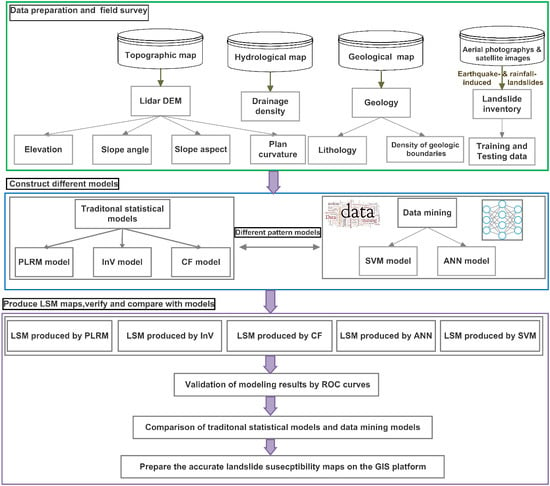
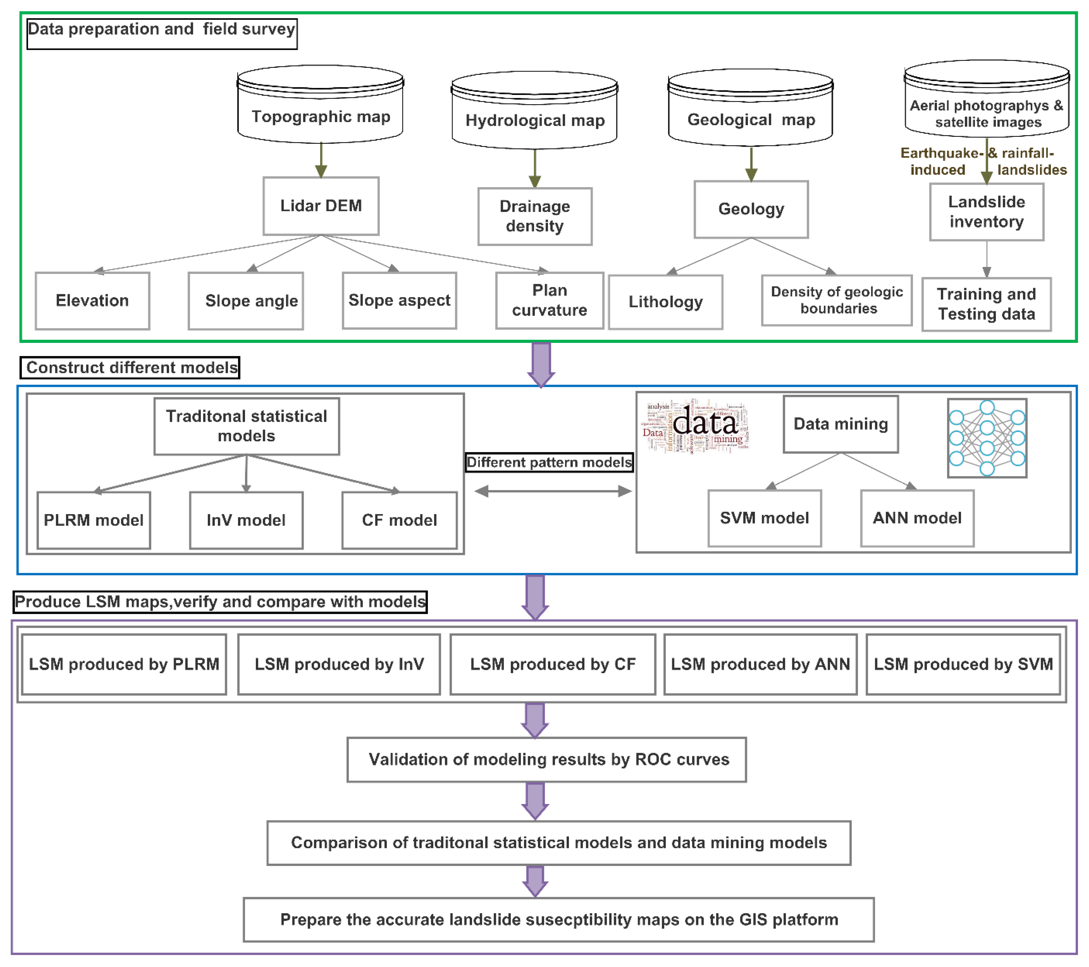
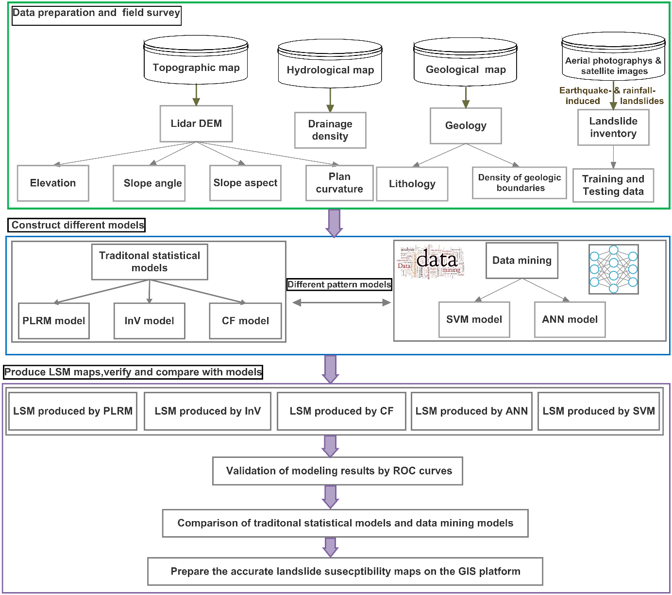
Our study is built upon this prior experience in different models to investigate the comprehensive performance of the susceptibility models using LiDAR DEM data. We address two research questions in this paper: (i) do the sophisticated data mining methods provide a better predictive competency compared with the traditional statistical methods? And (ii) how different the results while using multi-type landslides instead of single type landslides? For achieving the first objective, we analyze and compare the accuracy of LSM maps generated by five different techniques including three traditional statistical methods, that is, probabilistic likelihood-frequency ratio model (PLFR), information value (InV), certainty factor approach (CF); and the two machine learning techniques namely, artificial neural network (ANN) and support vector machine (SVM) in a regional-scale analysis. For achieving the second objective, we used the inventory of both earthquake-and rainfall-induced landslides in the analysis.

2. Overview of the Study Area

Landslides are frequently reported after earthquakes and rainfall events in the Chuetsu area, Niigata Prefecture, Japan [35]. This area has a steep mountainous topography and conducive geology that makes it inclined to severe landsliding [23]. Extensive landslides in this area are reported after two major seismic events; Chuetsu earthquake in 2004 and Niigata Chuetsu-Oki earthquake in 2007 [35,36]. 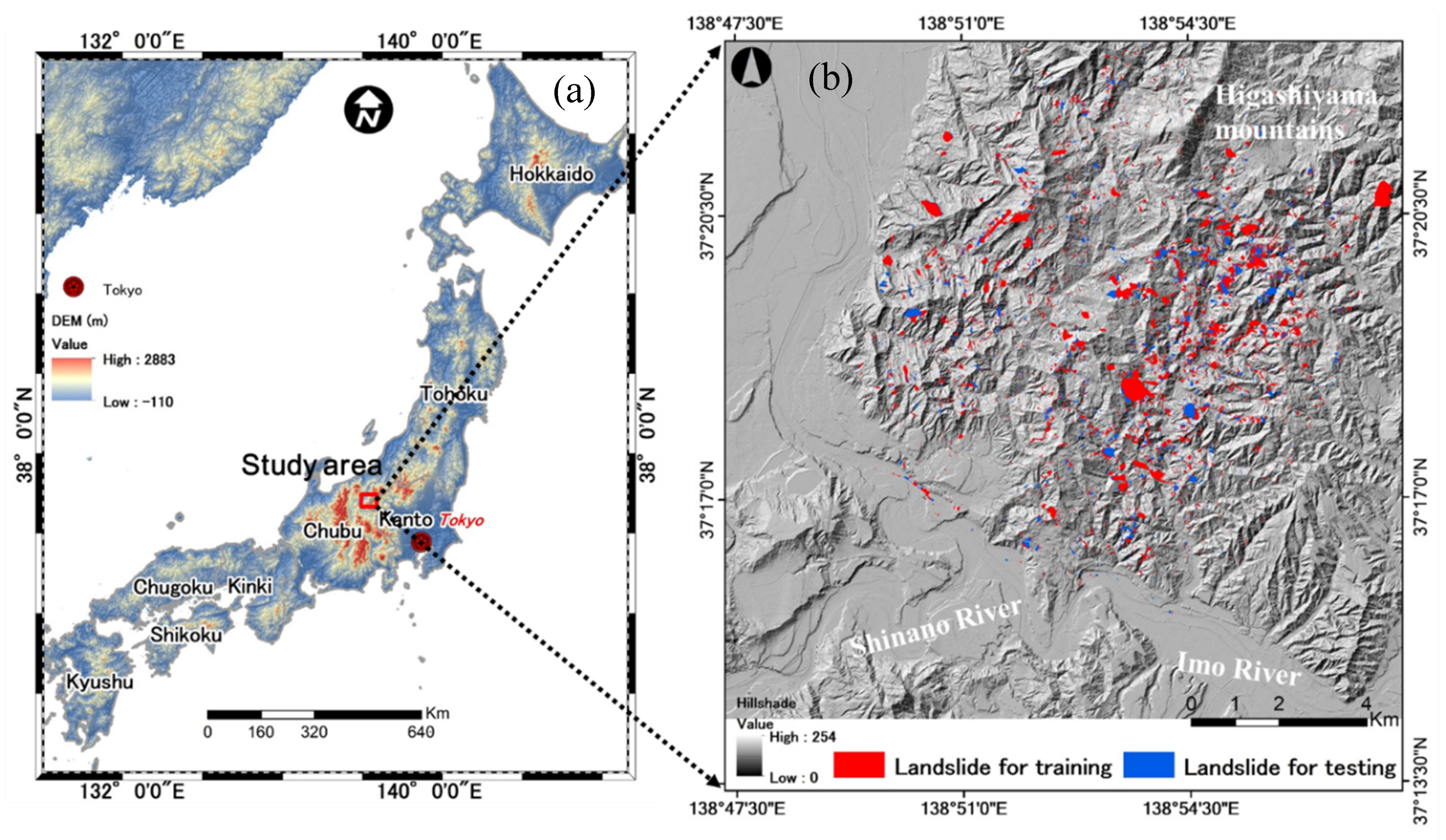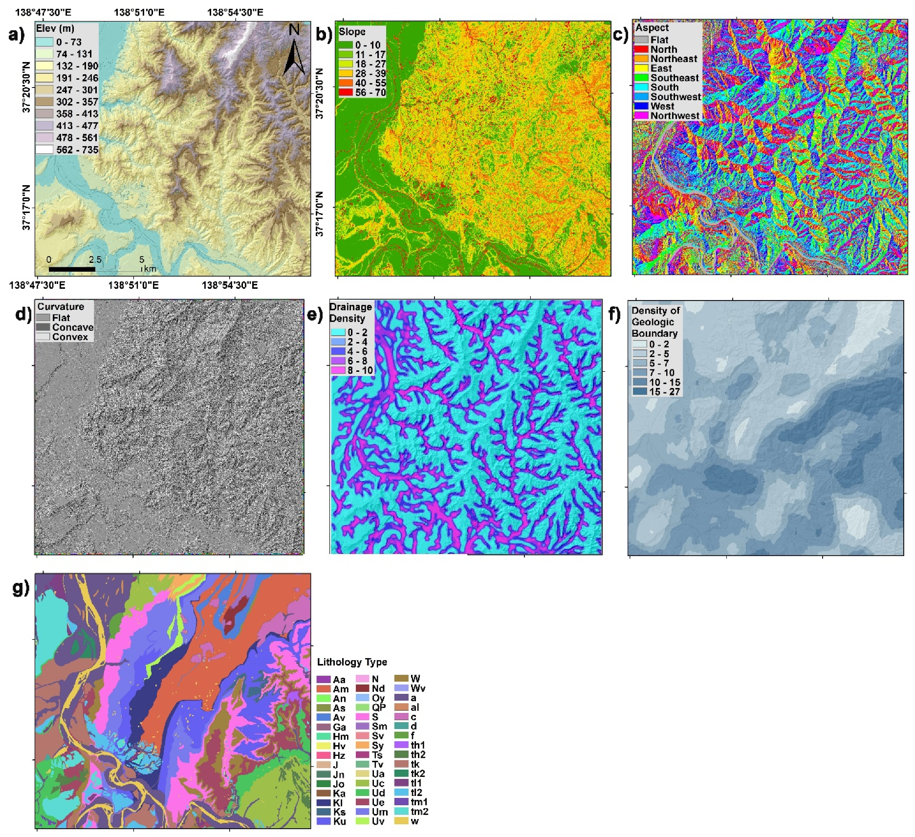The heavy rainfall in summers, typhoons and snow melting brought occasional debris movement as well [37]. The present work is carried out in an area within the Higashiyama hill region in the Niigata-Chuetsu region Japan (Figure 1) which covers approximately 290 km² area. The elevation ranges between 22 m and 734 m with an average elevation of 206 m above the sea level. The area receives an annual rainfall equaling 2000 mm, chiefly delivered by typhoons, as well as those during the summer and winter snow period from Japan Meteorological Agency.

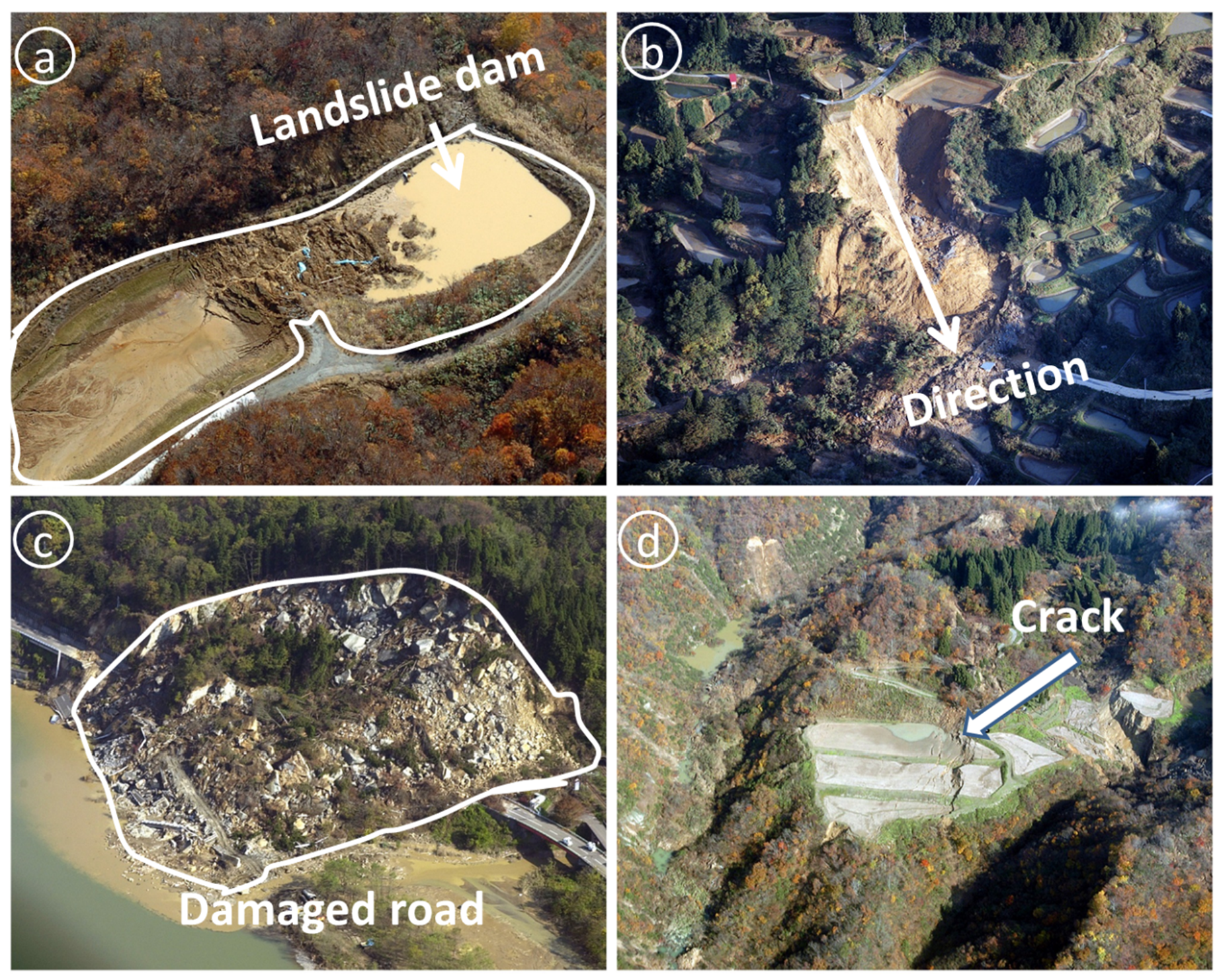
Metamorphic and sedimentary rocks belong to the Paleocene to the Quaternary period, as well as folded mountain belts distributed over NNE-SSE axes represent the geologic characteristic of the studied portion [38]. The epicenter of the 6.8 M Chuetsu earthquake of 2004 with the hypocenter at the depth of 13 km was located only a few kilometers away from the study region. This event also resulted in serious aftershocks in southern Higashiyama Mountain. Consequently, thousands of mass movement events occurred in the region (Figure 2). Numerous roads, houses, bridges and other infrastructures were severely damaged. The damages due to the event were largely concentrated on the Imo river basin the extent to which makes it necessary to assess similar hazards to mitigate the damages in the future.

3. Materials and Methods

The framework for the LSM in this research is depicted in Figure 3. Initially, the earthquake- and rainfall-induced landslides were delineated by interpreting multiple aerial photographs, satellite imageries and ground truths to construct a comprehensive landslide inventory for the study area. This database includes the landslide inventories provided by the National Research Institute for Earth Science and Disaster Prevention (NIED), Japan, as well as those prepared by the first author. Next, the relationship between landslide distribution and the causative mechanism were analyzed. Thereafter, the LSM maps were produced by traditional statistical models and data mining techniques, respectively. At last, the five models were examined and verified for accuracy using the receiver operating characteristic curve (ROC) function.

3.1. Landslide Inventory and Data Collection

The events in the past are significant in predicting the events in the future [39]. Thus, an inventory of past events is the most important information in mitigating any hazards [29,40]. A landslide multi-inventory database provides the geospatial coordinates of the past events, time of their occurrences and characteristics; this information is valuable for any methods of landslide risk or hazards assessment [29,34]. Furthermore, the quality and reliability of landslide data are also equally important as it will affect the subsequent results. This study uses the landslides inventory provided by the NIED, Japan as well as those prepared by the first author; both representing landslides as polygons feature class. A total of 8459 landslides triggered by the earthquake- and rainfall-induced landslides were used in susceptibility analysis. The landslides data were then randomly divided into a proportion of 70 and 30 for creating the LSM models and for validating the models, respectively. The total area of landslides covers an area of approximately 6.67 km², which is about 2.29% of the entire study area. We obtained the frequency–area distribution curve by plotting the landslide area (AL) data versus the probability density (P (AL)) values. The resultant frequency–area distribution exhibits a power-law with a good fit (R² = 0.99) as shown in Figure 4. This distribution displayed the segment for medium to large landslides with a visible rollover (at about 102 m²).

The resolution of DEM used in this analysis is a 2 m airborne LiDAR-derived product, which provides minute information such as scarp surface of landslides in detail. The post-earthquake LiDAR DEM of 2 m resolution with root-mean-square error (RMSE) within 0.12 m was produced from airborne LiDAR data surveyed in 2005, released by the GSI of Japan, 2007. The point density was greater than 1 pt/m² with a 70,000 Hz pulse rate frequency. The LiDAR technique has been proved as a valuable tool in the applications of geological engineering and monitoring ground movements, including the investigation of landslides [25]. The LiDAR DEM was obtained through the Geographical Survey Institute (GSI) data repository. The data pertaining to lithology and distance to the density of the geologic boundaries were prepared from the geological maps (scale 1:50,000) provided by Geological Survey of Japan-GSJ [38]. The details of data collection were given in

Table 1. Data collection in the study area.

Thematic Layer	Causative Factors	Data Type	Scale or Resolution	Classes	Producer	Description
Landslide inventory map	Landslide	Polygon	1:50,000	Continuous	NIED and interpretations	Landslide occurrence
Geological map	Lithology	Polygon	1:50,000	Non-continuous	Geological Survey of Japan	Type of lithology
	Density of geological boundary	Line		Continuous		Density of geologic unit
Topographic map	Elevation			Continuous	Geographical Survey Institute	Elevation-m
	Slope angle			Continuous		Slope degree
	Slope aspect	ARC/INFO	2 × 2 m	Continuous		Direction
	Plan curvature	Grid		Continuous		Concave or convex
Hydrological Map	Drainage density			Continuous		Density

.

3.2. Common Factors Controlling Earthquake- and Rainfall-Induced Landslides

The landslide causative factors are crucial significance for the LSM. Coseismic landslides are largely controlled by topographic, seismic and geologic factors [41,42,43]. Whereas the rainfall-induced landslides are dependent on climatic, topographic, as well as geologic factors [42,44]. In the present study, we analyzed the control of seven common landslide-causative parameters used in both earthquake-triggered as well as rainfall-induced landslides. This selection is based on the literature that discussed spatial relationships between landslide occurrence and causative parameters [34,41,43]. They are: (1) elevation, (2) slope angle, (3) slope aspect, (4) plan curvature, (5) drainage density, (6) lithology and (7) density of geologic boundaries. Each factor was classified into several sub-classes. The details of each class can be referred to Figure 5. The topographic related factors such as elevation, slope aspect, slope angle, drainage density and plan curvature were derived from the LiDAR DEM provided by the GSI. The geological factors like lithology and the density of geologic boundaries were prepared from the 1:50,000 geological maps of GSJ. All the factors were processed in a GIS platform ArcGIS 10.3. The brief delineation of each landslide causative factor map in the present study is given below.

3.2.1. Elevation

Central to most of the landslide susceptibility models is the elevation of the terrain and number of landslides [7,45]. It is the measure of height above the m. s. l., controlled and influenced the distribution of vegetation. A worldwide database of coseismic landslides by Tanyaş et al., (2018) [46] shows that approximately 80 percent of landslides are located between 100 m to 800 m elevation with a mean of 524 m. In the study area, the elevation ranges between 0 m and 735 m and the landslide largely occurred between 130 m and 413 m elevation ranges in Figure 5a.

3.2.2. Slope Angle

Slope angle refers to the inclination or rate of change in surface elevation for each pixel. Slope is an important variable that is found to affect the shear resistance, runoff rate and soil moisture and thus it is also one of the most significant factors affecting the stability of slope [30,47]. Typically, with an increased steepness, the number of landslides increases. However, it varies with the type of slides such as rock falls, shallow landslides and deep-seated landslides. The slope angle varied between 0°–70°. Most of the landslides were observed on the slope between 17° to 55°. This is consistent with the global landslide database of Tanyaş et al., (2018) [46] where 80% of landslides are found occurred between 10°–45° slope angle in Figure 5b.

3.2.3. Slope Aspect

Aspect indicates the downslope direction, it is also related to is related to the orientation of precipitation, exposure to sunshine and wind impact [40]. The relationship between aspect and landslide occurrences are identified in a number of studies [4,32]. Their studies indicate that aspect influences the distribution of landslide by the propagation direction of seismic waves. Further, aspect also relates to the slipping orientation of the seismogenic fault [41]. Also, when the hillsides suffer from the dense precipitation to reach saturation, it influences the infiltration properties of the ground, permeability, as well as pore water pressure. The peak landslide areal density is observed for South, South-East and South-West a sloping direction in Figure 5c.

3.2.4. Plan Curvature

Planform curvature or simply plan curvature delineates the morphology of the topography and is measured perpendicular to the orientation of the maximum slope [45,48]. This parameter is the divergence or convergence of water during downhill flow affecting the landslide occurrences. Ohlmacher (2007) [49] demonstrates that landslide hazard should properly address the complex association exists between plan curvature, landslide types and the landslide susceptibility. We grouped the plan curvature into two categories, that is, concave (negative value) and convex (positive value). There is no clear effect of curvature on landslide susceptibility, as both curvatures (convex and concave) have almost similar number of failures in Figure 5d.

3.2.5. Drainage Density

Drainage density (DD) network interplays the movement of landslide associated with infiltration of water. DD (m⁻¹) is the total length of the stream network in a drainage watershed divided by the watershed area. The stream channel networks are extracted from high-resolution LiDAR DEM data. A practical D8 algorithm has been widely used to compute the DD in the available ArcGIS environment [50]. Stream heads were assumed to be located where the drainage area is 0.1 km² following Hayakawa and Oguchi [51]. The extracted the stream network overlaid the Google Earth image for validating the quality and uncertainties of extraction from DEM data. Drainage network and drainage density are also an indirect measure of groundwater conditions. During any seismic event, the pore pressure built-up occurring in the vicinity could trigger coseismic landslides. Similar behavior can also be noticed during the excessive rainfall conditions when infiltration capacity exceeds a certain threshold. Several scholars proved the impact of the landslide process on geomorphological characteristics of the drainage network [34,45]. For instance, Oguchi (1997) [52] proved that there is a correlation between drainage density and landslide distribution (DL) in steep Japanese mountains. For this study, the peak landslide aerial density is observed for density class 6–9 in Figure 5e.

3.2.6. Density of Geologic Boundaries

Lithological boundaries are marked as the plane of discontinuity and generally are zones of weakness. They influence the rock strength. The higher value of the density of geologic boundaries indicates more susceptible to landslide occurrences. In the present study, the density of geological boundaries was computed from the geologic boundary data with the help of GIS software using a circle of 200 m radius as they are found appropriate in a study by Kawabata and Bandibas (2009) [53] for this location. The landslide density increases with the increased density of lithological boundary and the peak values are observed for class 15–27 in Figure 5f.

3.2.7. Lithology

Bedrock geology plays a significant role in the landslide failure and their distribution because different rock types and lithological units behave differently to alterations in the geomorphic process, permeability and strength of rocks and soils [7,37]. Influence of lithological control on landslide distributions in the Japanese archipelago has been noticed in several studies [37,41]. In the Higashiyama Mountain and its surroundings, lithology was classified into 35 categories (

Table 2. Classification of geologic substrata in the study area (revised from Takeuchi and Yanagisawa, 2004).

Geologic Age	Lithology	Geologic Unit
Holocene	Gravel, sand and silt	a
	Gravel and sand	al
	Debris, gravel and sand	d
	Gravel and sand	f
	Gravel, sand and silt	tk
Late Pleistocene	Debris and colluvial soil	c
	Gravel, sand and silt	tl2
	Gravel, sand and silt	tl1
Middle Pleistocene	Gravel, sand and silt	tm2
	Gravel, sand and silt	tm1
	Gravel, sand and silt	th2
	Gravel, sand and silt	th1
	Gravel, sand and mud	Oy
Late Pliocene–Early	Marine silt and sand	Ue
Pleistocene	Gravel, sand and silt	Ud
	Gravel, sand and silt	Uc
	Gravel and sand	tk2
Late Pliocene	Sandstone	W
	Sandy siltstone and alternation of sandstone and siltstone	S
Early Pliocene–	Andesite, dacite lava and pyroclastic rock	Ka
Late Pliocene	Tuffaceous sandstone and Andesitic pyroclastic rock	Sy
	Massive mudstone	Um
	Andesitic pyroclastic rock	Uv
	Sandstone	Ks
	Mudstone interbedded with sandstone	Ku
Late Miocene–	Sandstone interbedded with mudstone	Kl
	Andesitic pyroclastic rock	Av
Early Pliocene	Sandstone and alternation of sandstone and mudstone	As
	Massive mudstone	Am
Late Miocene	Dacite, andesite lava and volcanic breccia	Tv
	Massive mudstone	Ts
Middle Miocene–	Dacite lava and pyroclastic rock	Nd
	Andesitic pyroclastic rock	Sv
Late Miocene	Hard shale and alternation of sandstone and shale	Sm
(Water)		(w)

). In this case, the landslides mostly occurred at the age of Late Pliocene, Late Pliocene–Early, Marine Pleistocene, Late Miocene–Early Pliocene and the type of lithology, such as sand and silt, sandstone, massive mudstone, sandstone and alternation of sandstone in Figure 5g. Previous studies also reported a high number of landslide density in sedimentary rocks [34,37,41].

3.3. Methods

Different statistical methods have been used for individually producing a series of modeling of landslide susceptibility maps.

3.3.1. Probabilistic Likelihood-Frequency Ratio

Probabilistic likelihood-frequency ratio model (PLFR) is established on the assertive relationship flanked by the spatial distribution of landslides and each relative-causative factor, displaying the interrelation between the location of landslides and causal parameters affecting the landslides occurrence in a certain area [54,55]. In order to foresee the future landslides, the basic assumption is that the occurrence of landslides are largely controlled by certain landslide factors and the imminent landslides will also happen under the similar circumstances as the historical events [55].

According to the aforementioned assumption, the PLFR is the “ratio of the probability of landslide occurrence to the probability of non-landslide occurrence” for related factors’ attributes [54]. The PLFR is calculated for each factor from their relationship to landslide distributions. The higher the ratio value, the better the correlation between landslide incidence and the given causative factor [55]. A value of 1 and greater indicates that the particular class of landslide has a stronger relationship with the landslide occurrence. Otherwise, it has a lower correlation. PLFR is expressed as:

$$\mathrm{PLFR}=\left(\frac{\frac{\mathrm{No}.\mathrm{of}\mathrm{landslides}}{\mathrm{Total}\mathrm{of}\mathrm{landslides}}}{\frac{\mathrm{No}.\mathrm{of}\mathrm{landslides}\mathrm{in}\mathrm{domains}}{\mathrm{Total}\mathrm{of}\mathrm{pixels}}}\right)$$

(1)

$\mathrm{No}.\mathrm{of}\mathrm{landslides}$ and $\mathrm{No}.\mathrm{of}\mathrm{landslides}\mathrm{in}\mathrm{domains}$ represent the number of landslides in each class and number of landslides in each domain, respectively; $\mathrm{Total}\mathrm{of}\mathrm{landslides}$ and $\mathrm{Total}\mathrm{of}\mathrm{pixels}$ denote the total landslides and a total number of pixels in the entire the study area. And the landslide susceptibility index, LSI is the sum of the all ratios estimated for each causal factor. LSI thus provides a degree of certainty in forecasting landslides. Summation of each factor’s probabilistic likelihood-frequency ratios are calculated by the following equation:

$$\mathrm{LSI}={\displaystyle \sum }\mathrm{PLFR}=\mathrm{PLFR}1+\mathrm{PPFR}2+\dots +\mathrm{PLFRn}$$

(2)

where $\mathrm{PLFR}$ is the rating value of each factor. The greater the LSI value, the higher the risk of landslide occurrence and vice versa.

3.3.2. Information Value Method

The information value (InV) method has been successfully used in various field of geosciences, medicine, economy and biology [31]. With this bivariate statistical analysis method, each of the individual parameters is integrated with the landslide inventory database and weight of landslide density to each landslide causative factor class is then calculated.

For this approach, the landslide occurrence is regarded as a dependent variable and each causative factor influencing this condition is regarded as an independent variable. Aleotti and Chowdhury (1999) [15] showed that InV requires five steps: (1) selection of significant factors, their mapping and classification into a number of correlative groups; (2) their overlay analysis with landslide inventory database; (3) determine the landslide density for each causal factor; (4) assign weight to each causal factors; (5) finally calculate the eventual hazard based on the weighted values.

Bivariate statistical models are regarded to be a quantitative method in landslide hazard zonation, however, there exists a certain degree of subjectivity in the analysis. Additionally, it should be appreciated that in many cases, the employed factors may have a problem of high correlations, which causes the noise of resulting models [32,54].

The LSM is performed by applying InV method-statistical index (W_i) approach. The W_i (InV) approach is based on the statistical correlation between inventoried landslides and the attributes of various causative factors. The W_i value of each parameter is defined as the difference between the density of each parameter class and the average density of landslide [56]. W_i is calculates using the following equation:

$$W_i=\ln (\frac{\mathit{D}\mathit{e}\mathit{n}\mathit{s}\mathit{C}\mathit{l}\mathit{a}\mathit{s}\mathit{s}}{\mathit{D}\mathit{e}\mathit{n}\mathit{s}\mathit{M}\mathit{a}\mathit{p}})=\ln (\frac{\raisebox{1ex}{$\mathit{N}\mathit{p}\mathit{i}\mathit{x}\left(\mathit{S}\mathit{i}\right)$}\!\left/ \!\raisebox{-1ex}{$\mathit{N}\mathit{p}\mathit{i}\mathit{x}\left(\mathit{N}\mathit{i}\right)$}\right.}{\raisebox{1ex}{${\displaystyle \sum }\mathit{N}\mathit{p}\mathit{i}\mathit{x}\left(\mathit{S}\mathit{i}\right)$}\!\left/ \!\raisebox{-1ex}{${\displaystyle \sum }\mathit{N}\mathit{p}\mathit{i}\mathit{x}\left(\mathit{N}\mathit{i}\right)$}\right.})$$

(3)

W_i: the weight assigned to a causative parameter class (e.g., elevation, aspect, slope);

DensClass: the landslide density (LD) within this parameter class;

DensMap: the LD for the whole study area

Npix(Si): the total number of pixels that contains landslide in a certain parameter;

Npix(Ni): the total number of pixels contained in a certain parameter class;

Eventually, the LSM by InV model was produced by the subsequent equation:

$$\begin{array}{l}LS{M}_{wi}=\left(W{i}_{elevation}\right)+\left(W{i}_{slopeangle}\right)+\left(W{i}_{\mathrm{slope}\mathrm{aspect}}\right)\\ +\left(W{i}_{\mathrm{density}\mathrm{of}\mathrm{geological}\mathrm{boundary}}\right)+\left(W{i}_{\mathrm{drainage}\mathrm{densitys}}\right)\\ +\left(W{i}_{\mathrm{plan}\mathrm{curvature}}\right)+\left(W{i}_{\mathrm{lithology}}\right)\end{array}$$

(4)

3.3.3. Certainty Factors

The certainty factors (CF), a numerical value that articulates a measure of belief or the degree of certainty is a method widely used in rule-based systems for managing the uncertainty [7,33]. The CF technique deals with the problem of integrating heterogeneous data and therefore is considered as one of the probable favorability functions (FF). [57]. CF can be expressed as:

$$\mathrm{CF}=\{\begin{array}{l}\frac{{\mathrm{PP}}_{\mathrm{a}}-{\mathrm{PP}}_{\mathrm{s}}}{{\mathrm{PP}}_{\mathrm{a}}*\left(1-{\mathrm{PP}}_{\mathrm{s}}\right)} \mathrm{if} {\mathrm{PP}}_{\mathrm{a}}\ge {\mathrm{PP}}_{\mathrm{s}}\\ \frac{{\mathrm{PP}}_{\mathrm{a}}-{\mathrm{PP}}_{\mathrm{s}}}{{\mathrm{PP}}_{\mathrm{s}}*\left(1-{\mathrm{PP}}_{\mathrm{a}}\right)} \mathrm{if} {\mathrm{PP}}_{\mathrm{a}}<{\mathrm{PP}}_{\mathrm{s}}\end{array}$$

(5)

where, ${\mathrm{PP}}_{\mathrm{a}}$ is the conditional probability of having a number of landslide events occurring in class a and ${\mathrm{PP}}_{\mathrm{s}}$ is the prior probability of having a total number of landslide events in the study area. We found the PPs in the study area as 0.26.

The CF value is calculated for each class layer using Equation (5). These layers are then integrated pairwise based upon the parallel-combination rule given in the following equation [33]:

$$\mathrm{Z}=\{\begin{array}{lll}\mathrm{CF}1+\mathrm{CF}2-\mathrm{CF}1\mathrm{CF}2& \mathrm{CF}1,& \mathrm{CF}2\ge 0\\ \mathrm{CF}1+\mathrm{CF}2+\mathrm{CF}1\mathrm{CF}2& \mathrm{CF}1,& \mathrm{CF}2<0\\ \frac{\mathrm{CF}1+\mathrm{CF}2}{1-\min \left(\left|\mathrm{CF}1\right|,\left|\mathrm{CF}2\right|\right)}& \mathrm{CF}1,& \mathrm{CF}2,\mathrm{opposite}\mathrm{signs}\end{array}$$

(6)

The pairwise combination is operated until all the CF layers are brought together. The CF values range between −1 and +1 in which −1 indicates false and +1 indicate true. A positive CF corresponds a high certainty of landslides, while a negative CF corresponds to a low certainty of landslides. A value of zero corresponds to conditional probability similar to prior probability and hence difficult to determine the certainty [7].

3.3.4. Artificial Neural Network

Artificial Neural Networks (ANN) based on data mining techniques is known as a popular artificial intelligent method used to solve many problems of real worlds such as modeling nitrate pollution of groundwater [58], prediction of wind speed and wind direction [59] and forecasting the blast-produced ground vibration [45]. Furthermore, ANN is widely used in landslide modeling and mapping previously [53,60]. The principle behind ANN is defined on the behavior of the human brain in which learning algorithms are used for classification and prediction. It uses the average of the weighted sum of numerous sigmoid to define a decision function. In ANN modeling, the back-propagation technique is the typically used error distribution criteria to train the neural networks because of its flexible and adaptive ability [60].

In landslide prediction, the structure of the ANN includes a three-layer neural network as shown in Figure 6; an input neuron, a hidden neuron and an output neuron, where input neurons represent the landslide causative factors (slope, aspect, etc.), hidden neurons represent the activation function utilized for driving the input neurons to forecast output neurons and output neurons represent predictive variables (non-landslide or landslide) [61]. The backpropagation ANN empowered training by defining the weights of each causative factor. This trained algorithm was then used first for testing the data during the classification stage, which then omitted during the training period. Weights are defined by altering the number of hidden neurons and the learning curve between the input and hidden layers and between the hidden and output layers.

To opt the proper number of hidden neurons, the neurons were randomly set and performed in ten times of network to select the average value of R² for decreasing the effect of the initial value in the ANN model.

Let $u=\left(u_1,u_2,\dots ,u_n\right)$ represent n input neurons whereas $v=\left(v_1,v_2\right)$ represent output neurons. For prediction of landslides, the activation function used in hidden neurons is expressed as follows:

$$v=f\left({\displaystyle \sum _{i=1}^n{\omega }_i}{u}_i+{\beta }_{}\right)$$

(7)

where ${\omega }_{ji}$ are defined as the connection weights between input neurons $u_i$ and output neurons v and $\beta$ are defined as the bias. The detailed parameter settings can be referred to the

Table 3. The setting variables in the artificial neural network (ANN) model.

Variables	Variables Setting
Root mean square error (RMSE)	0.001
Initial weights	0.1–0.25
Learning rate	0.01
Number of epochs	3000 iterations
Momentum parameters	0.9
Activation (transfer) function for layers	Transig for hidden layer, purelin for the output layer

.

3.3.5. Support Vector Machine

Support vector machine (SVM) is a high-performing supervised machine learning technique based on statistical learning theory, in which the input space is mapped to a feature space and then, in the feature space, a hyperplane is constructed to differentiate classes (e.g., the presence and absence of landslides) [62]. Typical SVM is divided into the two-class and multi-class SVM (grouping of a chain of two-class SVM). According to the literature, two-class SVM is the most commonly used model [10,23]. The details of two-class SVM can be referred studies. Figure 7 illustrates the scheme of SVM principle in which circle and squares denote two–class samples. In order to classify linearly, the kernel function converts the input samples into a high-dimensional space. The separating hyperplane (H) is one of the probable planes for separating the two classes; the space between the two dotted lines in the so-called margin.

In a landslide application, consider a set of training vectors xi; the classes denoted as y_i = ±1 (i = 1, 2…n). The landslides and non-landslide points are in the input space for originally converting nonlinear data to a linearly separable data with the support of an optimum separating hyperplane. SVM find an optimal hyperplane by differentiating the classes using the optimization function [62]:

$$\underset{w,b,\xi }{\overset{}{Min}}:\frac{1}{2}{w}^{T}w+c{{\displaystyle {\sum }_{i=1}^1\xi }}_i$$

(8)

Subjected to the constraints mentioned in the equation:

$$\begin{array}{l}{y}_i(w^T\mathsf{\varphi }(x_i)+b)\ge 1-{\xi }_i\\ {\xi }_i\ge 0\end{array}$$

(9)

where, w represents a coefficient vector, b represents the offset of the hyperplane from the origin,  represents the positive slack variable, c (> 0) represents the penalty variable of the errors; and the kernel function is expressed as:

$$k(x_i,x_j)=\mathsf{\varphi }{(x_i)}^T\mathsf{\varphi }(x_j)$$

(10)

Four types of kernels in SVM are linear, polynomial, radial basis function and sigmoid. The corresponding equations are listed below:

$$\mathrm{Linear}\mathrm{function}\left(\mathrm{LF}\right):k\left(x_i,x_j\right)=x_i^T{x}_j$$

(11)

$$\mathrm{Polynomial}\mathrm{function}\left(\mathrm{PF}\right):k\left(x_i,x_j\right)={\left(\mathsf{\gamma }{x}_i^T{x}_j+\mathsf{{\rm Y}}\right)}^d,\mathsf{{\rm Y}}>0$$

(12)

$$\mathrm{Radial}\mathrm{basis}\mathrm{function}\left(\mathrm{RBF}\right):\left(x_i,x_j\right)=\exp \left(-\mathsf{\gamma }|x_i-x_j{|}^2\right),\mathsf{{\rm Y}}>0$$

(13)

$$\mathrm{Sigmoid}\mathrm{function}\left(\mathrm{SF}\right)k\left(x_i,x_j\right)=\tan h\left(\mathsf{\gamma }{x}_i^T{x}_j\right)+\mathsf{{\rm Y}},\mathsf{{\rm Y}}>0$$

(14)

where $\mathsf{{\rm Y}}$ and $\mathsf{\gamma }$ denote factors of kernel functions. During these four types of kernel functions, RBF usually provides a better predictive capability for LSM than other kernel functions in non-linear classification [23,63]. Additionally, a novel ensemble model was proposed by integrating normalized InV values from the bivariate analysis with BF-SVM kernel. Thus, in this study, RFB coupled with InV method was used to implement to produce LSM. Finally, five LSM maps were created on the platform of ArcGIS 10.3 into five classes (Very low, Low, Moderate, High and Very high) based on the natural break classification approach which is good when there are big jumps in data values.

3.4. Accuracy Assessment of the Models

All susceptibility models must be verified for their accuracy of predictions. An unverified prediction model and susceptibility maps are nonetheless meaningless and hence do not have any scientific significance [57]. Several studies have addressed the issue of LSM validation [13,64].

Most commonly, the models are verified with an independent set of data that was not used for training the model. Irigaray et al. (2006) [65] and others reported a three following approach to obtain an independent sample of the landslide for validation purpose.

From the total landslide inventory map of the study area, create two sets of randomly divided landslide polygons, one for the susceptibility analysis and one for validation the models;

The susceptibility analysis should be performed in a part of the whole study area; the obtained result should be tested in another part, distinctly with different landslides;

The analysis should be carried using landslides occurred in a certain period and validation should be performed by means of landslides occurred in a different period. This is the most sufficient to test the validity of the “prediction” mode, however, the toughest to apply as it needs knowledge of the temporal distribution of landslides during adequately long-time spans.

In this study, we applied the first approach to validate the LSM map that has been proposed by some works [45]. Validating models are tested by receiver operating characteristics (ROC). ROC is found to be a very valuable indicator to evaluate the superiority of deterministic and probabilistic detection and forecast systems [66,67,68]. The resultant ROC curve demonstrates the performance of the classifier system by plotting the fraction of false positive out of the entire actual negatives (FRP = false positive rate) versus the fraction of the true positive out of the entire actual positive (FPR = true positive rate) as its discrimination threshold is varied in

Table 4. Contingency table of calculation of ROC curve.

Total Number		Event		Sum
		Condition Positive	Condition Negative
Test result	Positive	True positive (TP)	False positive (FR)	TP + FR
	Negative	False negative (FN)	True negative (TN)	FN + TN
Sum		TP + FN	FR + TN	TP + FR+ FN+ TN

. The area under the ROC curve (AUC) can characterize the quality of a forecast system by describing the system’s ability to correctly predict the occurrence or non-occurrence of a predefined event. It is a curve measured the sensitivity-y-axis and the 1-specificity x-axis gained by the error matrix.

$$\mathrm{Y}=\mathrm{Sensitivity}=\left({\displaystyle \sum }\mathrm{True}\mathrm{positive}\right)/\left({\displaystyle \sum }\mathrm{Condition}\mathrm{positive}\right)=\mathrm{TN}/\left(\mathrm{TN}+\mathrm{FP}\right)$$

(15)

$$\mathrm{Specificity}=\frac{{\displaystyle \sum }\mathrm{True}\mathrm{negative}}{{\displaystyle \sum }\mathrm{Condition}\mathrm{negative}}=\mathrm{TN}/\left(\mathrm{TP}+\mathrm{FN}\right)$$

(16)

$$\mathrm{X}=1-\mathrm{Specifity}=1-\frac{{\displaystyle \sum }\mathrm{True}\mathrm{negative}}{{\displaystyle \sum }\mathrm{Condition}\mathrm{negative}}=1-\frac{\mathrm{TN}}{\mathrm{TP}+\mathrm{FN}}$$

(17)

The AUC can be calculated by the trapezoidal rule of integral calculus. The AUC value varies from 0.5 to1.0. The ideal model would have an AUC value of 1.0. According to Yilmaz (2009), the relationships between the accuracy ratings and AUC are usually listed as followed

Table 5. The accuracy ratings of AUC value.

Rank	Range	Description
1	0.9–1	Excellent
2	0.8–0.9	Good
3	0.7–0.8	Acceptable
4	0.6–0.7	Poor
5	0.5–0.6	Failed

.

4. Results

4.1. Modeling Result with the Probabilistic Likelihood-Frequency Ratio

The relationship between the spatial location of the landslides and landslides causative factors are processed as shown in

Table 6. Spatial relationship between the relative factors and landslides by CF, PLFR and InV models.

Factors	Class	Percentage of Domain (%)	Percentage of Landslides (%)	CF	PLFR	Wi (InV)
Elevation (m)	0–73	18.14	1.01	−0.96	0.06	−0.2
	73–131	17.67	6.86	−0.68	0.39	1.41
	131–190	15.36	19.96	0.31	1.3	2.71
	190–246	13.49	23.37	0.57	1.73	2.98
	246–301	11.65	19.35	0.54	1.66	2.94
	301–357	8.73	15.23	0.58	1.74	2.88
	357–413	6.57	9.32	0.4	1.42	2.66
	413–477	4.89	4.23	−0.17	0.87	1.74
	477–561	2.67	0.51	−0.85	0.19	0.5
	561–735	0.84	0.15	−0.86	0.18	−0.42
Slope angle (°)	0–10	39.37	4.72	−0.91	0.12	−1.25
	43390	12.91	9.74	−0.3	0.75	0.01
	17–27	19.62	22.17	0.17	1.13	0.36
	27–39	21.75	39.42	0.61	1.81	0.52
	39–55	6.2	23.82	1	3.84	0.57
	55–70	0.16	0.14	−0.18	0.85	0.42
Slope aspect	Flat	17.97	7.72	−0.88	0.85	1.81
	Northeast	9.5	6.34	−0.4	0.67	2.21
	East	10.06	11.12	0.13	1.11	2.48
	Southeast	9.7	15.01	0.48	1.55	2.66
	South	9.19	15.76	0.57	1.71	2.76
	Southwest	10.34	15.73	0.47	1.52	2.66
	West	11.99	14.15	0.21	1.18	2.54
	Northwest	11.78	8.98	−0.3	0.76	2.25
	North	9.48	5.19	−0.53	0.55	2.08
Plan curvature	Concave	57.46	49.49	−0.18	0.89	2.27
	Convex	42.54	50.51	0.21	1.15	2.53
Drainage density	0–2	27.24	21.25	−0.31	0.78	1.97
	2–4	27.24	28.66	0.02	1.05	2.35
	4–6	24.57	29.89	0.2	1.22	2.63
	6–9	15.45	17.28	0.1	1.12	2.55
	9–20	5.5	2.92	−0.56	0.53	1.77
Density of geological boundary	0–2	30.82	15.59	−0.58	0.51	1.6
	2–5	20.67	21.73	0.03	1.05	2.34
	5–7	20.79	25.26	0.21	1.22	2.52
	7–10	15.13	18.19	0.19	1.2	2.51
	10–15	9.47	14.13	0.42	1.49	2.82
	15–27	3.13	5.09	0.5	1.63	3.31
Lithology	w	3.22	1.05	−0.68	0.33	1.8
	Av	2.07	2.34	0.34	1.13	2.28
	Um	6.63	13.34	0.78	2.01	3.09
	a	13.87	0.49	−0.97	0.04	−0.86
	Sy	1.78	1.47	−0.04	0.83	2.01
	Kl	3.26	6.21	0.75	1.91	3.13
	Uv	1	2.49	0.89	2.49	3.25
	Am	10.81	19	0.7	1.76	3.11
	Ka	0.37	0.01	−0.97	0.04	−2.04
	Ku	7.74	21.41	0.94	2.76	3.71
	Oy	0.08	0.01	−0.86	0.16	1.27
	tk2	0.39	0	−1	0	0
	al	0.41	0	−1	0	0
	Uc	7.23	0.72	−0.91	0.1	0.44
	f	0.89	0.11	−0.89	0.12	1.76
	tm2	2.22	0.09	−0.96	0.04	−1.72
	tl1	0.76	0	−1	0	−2.77
	S	10.01	12.9	0.46	1.29	2.88
	Ud	2.86	0.72	−0.76	0.25	0.1
	tl2	2.51	0.49	−0.82	0.19	1.2
	c	2.17	2.14	0.22	0.98	2.37
	As	0.08	0.26	1	3.27	3.12
	W	5.77	8.01	0.52	1.39	2.8
	Sm	0.56	0.04	−0.94	0.07	−2.88
	Nd	0.58	0.31	−0.44	0.54	1.53
	th2	1.13	0	−1	0	0
	tk	5.41	0.03	−1	0.01	−3.89
	Ue	4.59	3.76	−0.05	0.82	2.35
	tm1	0.09	0	−1	0	0
	d	0.13	0	−1	0	0
	Tv	0.7	0	−1	0	0
	th1	0.17	0.19	0.33	1.12	2.44
	Ks	0.5	2.42	0.82	4.86	4.1
	Ts	0.01	0	−1	0	0
	Sv	0	0	−1	0	0

. According to Table 6, the PLFR values of elevation classes are greater than 1 at the ranges of 131–190 m, 190–46 m, 301–357 m, 357–413 m with the highest value (1.74). The results show that PLFR values increase with increasing altitudes till it reaches 357 m elevation in the study area. Its values drop further and become less than 1 after 413 m. This means that the possibility of landslide occurrence increases till it reaches a certain height and then decreases when the altitude is higher than 413 m.

With slope angle factor, PLFR values are greater than 1 from 17° to 55°. The landslide occurrence in the slope classes 17°–27°, 27°–39° and 39°–55° are 22.17%, 39.42% and 23.85%, respectively. Following the general trend, it can be seen that the occurrence of landslides progressively increases with an increasing slope. The percentage of landslide occurrences drops sharply after reaching the 55° slope angle. According to the results, it is clear that almost the landslide occurrence increases from one slope gradient up to a certain extent and then it decreases. The shear stress of the soil usually increases following with increasing slope angle.

For the aspect class, the significant number of landslides happened among east, southeast, south, southwest and west-facing directions, their frequency ratio value is all greater than 1. It indicates that the direction from east to west is highly susceptible to the landslide occurrence. A plausible explanation for this condition is that from east to west facing directions are general concerning fully rock weathering. Therefore, around these directions are susceptible to occur landslides.

For the plan curvature, the PLFR value of convex (1.15) has a large value than 1, while concave value (0.89) is less than 1. The results show that many landslides occurred at the convex areas.

The causative factor of drainage density (DD) has a larger value than 1 with the range of 2–4, 4–6 and 6–9. The maximum PLFR value is 1.12. Otherwise, the density of DR is greater than 9, the PLFR value becomes less than 1 and it has a lower probability of landslide occurrence.

In the case of the lithology, it is clear to see that the frequency ratios of Av, Um, KI, Uv, Am, Ku, S, As, W, Tv, th1, Ks are all more than 1. According to the investigation of lithological conditions, the landslides occurred mostly in the sandstone, massive mudstone, sandstone, gravel, sand and silt area corresponded with positive PLFR values.

In the case of the density of the geological boundary, from the 2–27, the PLFR values are higher than 1. The maximum PLFR value is 1.63 and the followed value is 1.49. The largest and second largest probabilities of landslide occurrence are 25.26%, 21.73% respectively. The density of geological boundary is less than 2 and the PLFR value is less than 1 which indicates that a lower percentage of landslide occurs in the density of geological boundaries.

4.2. Modeling Result with the Information Value (InV)

The result of the information value method and the relationship between the spatial location of the landslides and landslides causative factors are processed as shown in Table 6. According to Table 6, the InV values of elevation classes are susceptible at the ranges of 131–190 m, 190–246 m, 301–357 m, 357–413 m with the highest value (2.98), followed by 2.94 and 2.88. Results show that InV values decrease with the decreasing and increasing altitude in the study area. These results are similar to and PLFR’s results.

Regarding slope angle factor, the highest InV value is 0.57 from 39°–55°, followed by 0.52 from 27°–39°. The landslide occurrence in the slope classes, 27°–39° and 39°–55° are 27.97%, 36.7%, respectively. Again, what is observed similar to the PLFR, results of InV also shows that the occurrence of landslides gradually increases with an increasing slope angle until it drops after 55° slope angle due to the relatively lower percentage of the total study area. According to the results, it is clear that almost the occurrence of landslides increases from one slope gradient up to a certain extent and then it decreases because of increasing the shear stress of the soil with increasing slope angle. Therefore, the gentle slope has a relatively lower frequency of landslide occurrence because of the lower shear stress corresponded with a lower gradient. The steep slope angle normally causes the collapse to occur.

For slope aspect, landslides were prone to occur in the East, SE, South, SW and West facing slopes. The highest W_i value is 2.76 in the south direction, the following 2.66 in the south-east and south-west direction. To the density of geological boundary, as its values increases, the W_i values also increases that means more landslides occurred. The maximum W_i value 3.31 is obtained for the class with densest geological boundary (15–27) followed by a value of 2.82 in the lower geological density class (10–15). The greater density of geological boundaries indicates a plane of weakness or zone of discontinuity that leads to instability of rock bodies.

For the plan curvature, the value of convex (2.53) is a little larger than the value of concave (2.27). In concave and convex, the percentage of landslide occurrences is very close (51%, 49%, respectively). The drainage density shows that W_i value for 2–4, 4–6 and 6–9 are greater than 2. The W_i maximum value is 2.63 observed with 4–6 DD class. The highest percentage of landslide occurrences, 32.51%, also relates to the same DD class followed by 27.04% of the 2–4 DD class. The results of the lithology show that landslide is susceptible to in these types, namely massive mudstone, sandstone and alternation of sandstone and mudstone.

4.3. Modeling Result with the Certainty Factors

In Table 6, positive values of CF close to one are observed for the elevation classes 131–190 m, 190–246 m, 246–301 m and 301–357 m equaling 19.96%, 23.37%, 19.35% and 15.23%, respectively. It can also be seen from Table 6 that for an altitude of 190 m to 357 m, the CF values are greater than 0.5. This suggest that landslides are frequent in the mid-altitude and therefore their CF values; We observed that the ratio total pixels documented in mid-altitude are greater than that in the higher altitudes; whereas lower elevated areas are having the gentle slope and thus are not prone to landslides.

For slope class, CF values are found close to one from 17° to 55° class. The spatial distribution of landslides in the slope classes 17°–27°, 27°–39° and 39°–55° are 22.17%, 39.42% and 23.85%, respectively. Similar to PLFR and InV, the results are consistent for CF also which shows a gradual increase of landslide percentage till it reaches the slope angle 55°.

For aspect class, most of the landslide occurrences are found in the East, SE, South, SW and West facing slopes with a CF value between 0.13 and 0.57. The maximum percentage of landslides is found along the southern slope followed by SW slopes, equaling 15.76% and, 15.73%.

Curvature, the second derivate of the slope, provides valuable information on landslide occurrences. In this study, the CF corresponding to concave curvature gives a negative (−0.18) value, whereas the convex curvature corresponds to a positive (0.21) value. In most cases, the convexity indicates a low CF value than the concavity because of more water retention capacity in concave slopes which increases the soil moisture content that ultimately reduces the soil stability. Contrary to this, we found that concavity is not responsible for the landslide occurrences in this study region because most of the landslides are seismically induced. Mountaintops tend to collapse in coseismic cases because of topographic amplification differences.

A positive CF is recorded for the drainage density (Dd) classes 2–4, 4–6 and 6–9. The maximum CF is recorded for the study area is 0.2 which is observed for the Dd class 4–6, corresponding to 29.89% of landslide occurrences. As mentioned before, the largest chunk of landslides in Chuetsu-Niigata inventory is collected for the 2004 earthquake, the observed CF values are comparatively very small, which confirms the results.

CF values are found strong positive for the following lithology classes: Sandstone and alternation of sandstone and mudstone from Late Miocene–Early Pliocene (As); mudstone interbedded with sandstone (Ku), Andesitic pyroclastic rock (Uv), sandstone (Ks), massive mudstone (Um), sandstone interbedded with mudstone (KI) from Early Pliocene-Late Pliocene; and Massive mudstone (Am) from Late Miocene–Early Pliocene equaling 1.0, 0.94, 0.89, 0.82, 0.78, 0.75, 0.70, 0.52, respectively. The highest percentage of landslides among the lithology classes, 21.4%, occurred in Ku, followed by Am (19%) and Um (13.34%). The bedrock in the area of major landsliding consists of a folded sequence of sandstone, mudstone and their interbedding and the results point to the occurrence of landslides in the weakly cemented lithological groups.

We found that the CF values are always positive for the density of the geological boundary. The maximum CF is observed for the class 15–27 equaling 0.5; followed by the class 10–15 equaling 0.42. The percentage distribution of landslide occurrences in the above-mentioned classes is 25.26% and 21.73%, respectively. The negative CF value of the geological-density class lower than 2 indicates that geological uniformity affects the stability of the area. The higher density of geological boundaries suggests frequent process activity which leads to instability.

4.4. Modeling Result with the ANN

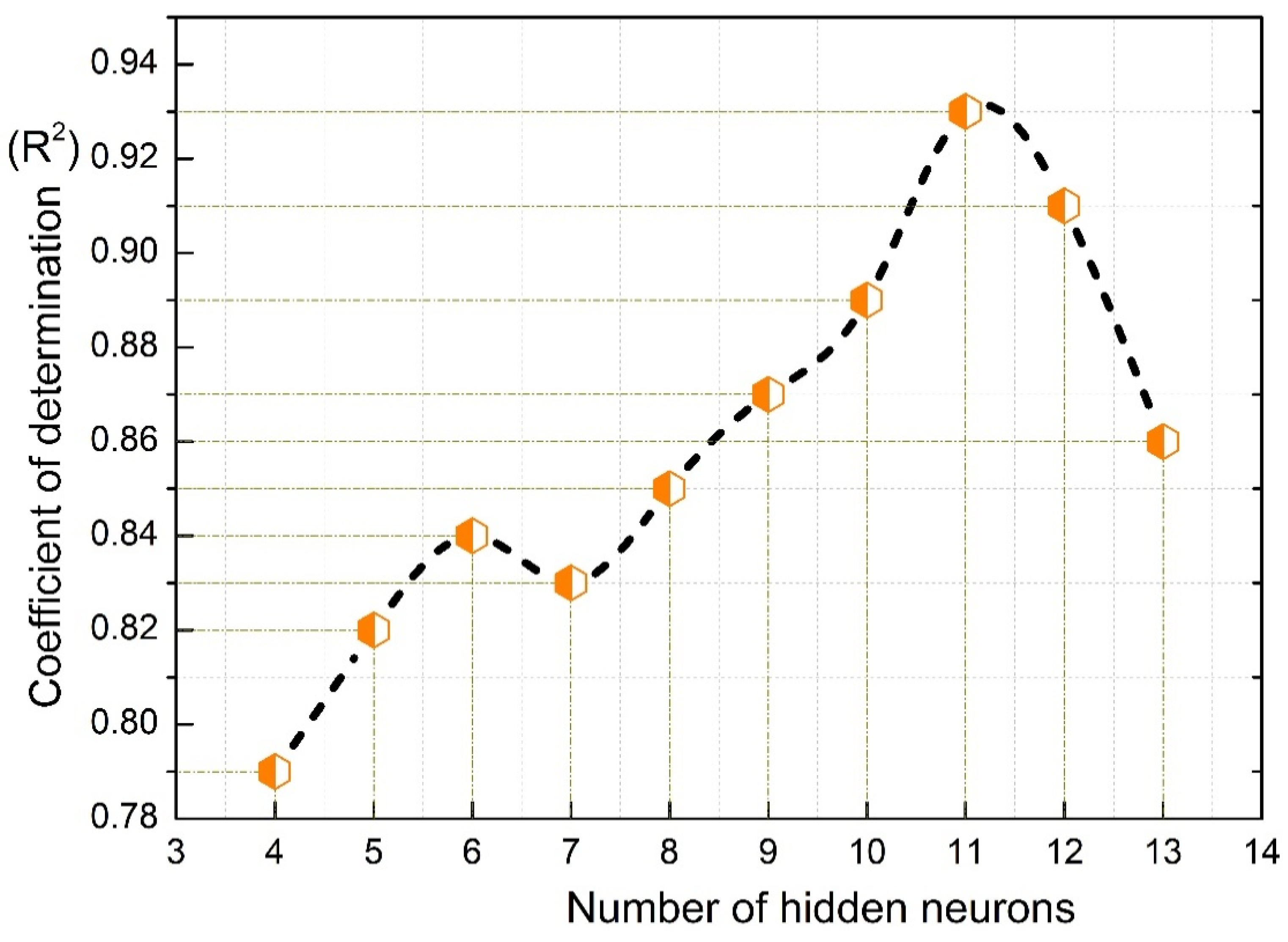
From Figure 8, it can be observed that when the number of hidden neurons is 12, R² has the highest values (0.92). The structures of the ANN (input–hidden–output) were set as 7–12–1. The weights between each layer were acquired by training the ANN to calculate the contribution of each landslide causative factor.

To examine the robustness of the ANN model, it was repeated 10 times, each with a random set of landslide data nominated from the whole data pool. There were no much variances in the results. The standard deviation was 0.0029. Thus, the random sampling sets did not have an obvious effect on the results. In this study, the average values were calculated to interpret the results. When the ANN achieved the minimum RMSE values (0.001), the whole pixels of the study area was fed into the ANN network to evaluate the LSM map. The final weights for the smallest error were documented in the procedure and weights of each factor were fixed for the entire study area. The sets of landslide susceptibility index values attained in all pixel were then converted into raster in GIS setting.

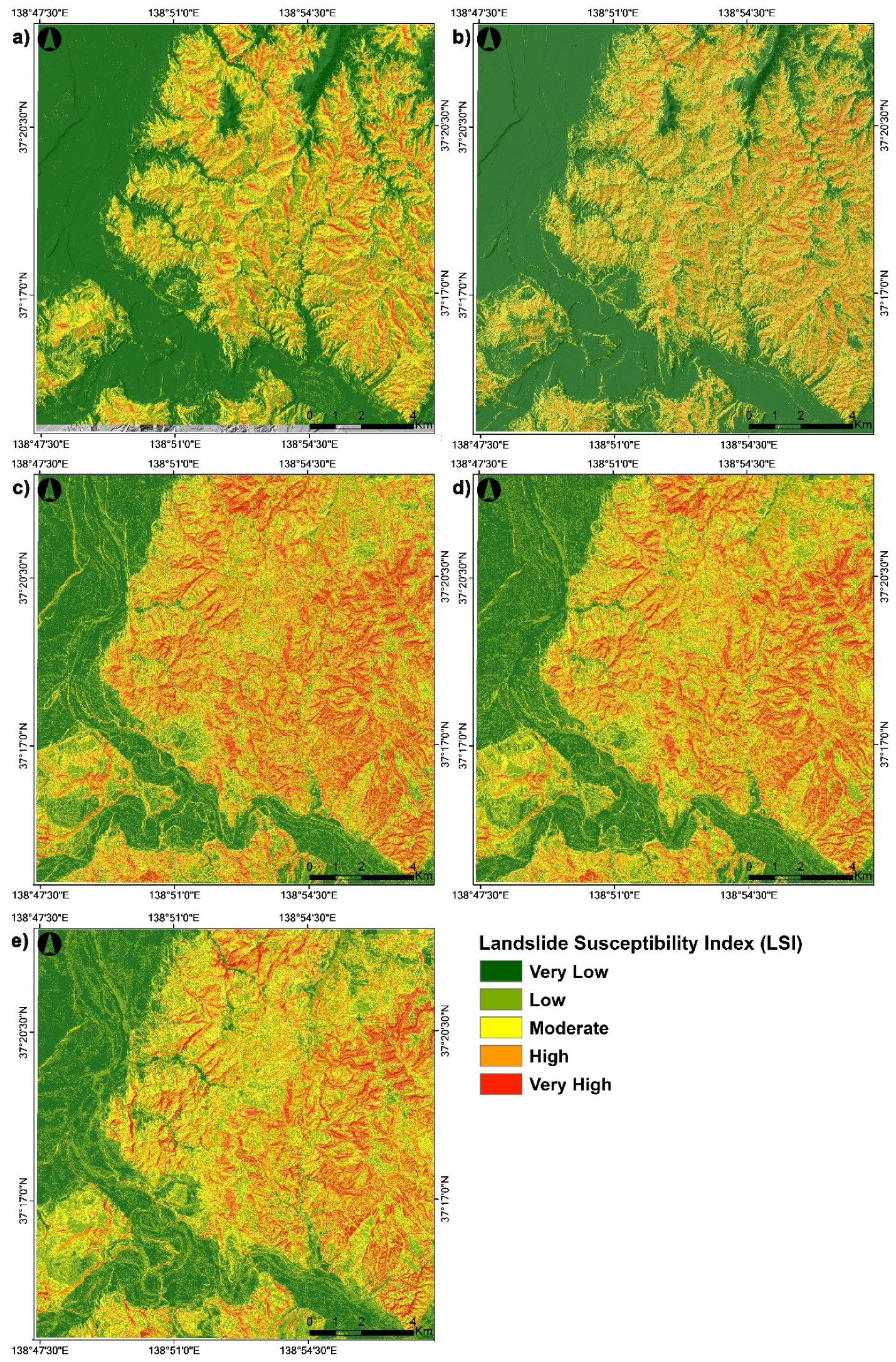
4.5. Modeling result with the SVM

The RBF applied in this model used the subsequent factors: γ = 0.5 and C = 10, convergence epsilon = 0.003 and maximal iterations = 5000. The results of the scenarios were next analyzed to decide the optimal kernel resulting in the best predictive capability. In this study, the RBF-SVM integrated with the InV method was selected for the improvement of the LSM map. The likelihood of landslide occurrence drops in the range from 0 to 1 that was transferred into the ArcGIS 10.3 package for visualization. Finally, the landslide susceptibility index values were reclassified into five classes: very low, low, moderate, high and very high using the natural break method, for easier visual clarification of the LSM. Figure 9. shows the spatial likelihood of landslide occurrences with the five classes, from very low (dark green) where landslides are not anticipated to very high (red) where landslides are possible using five methods.

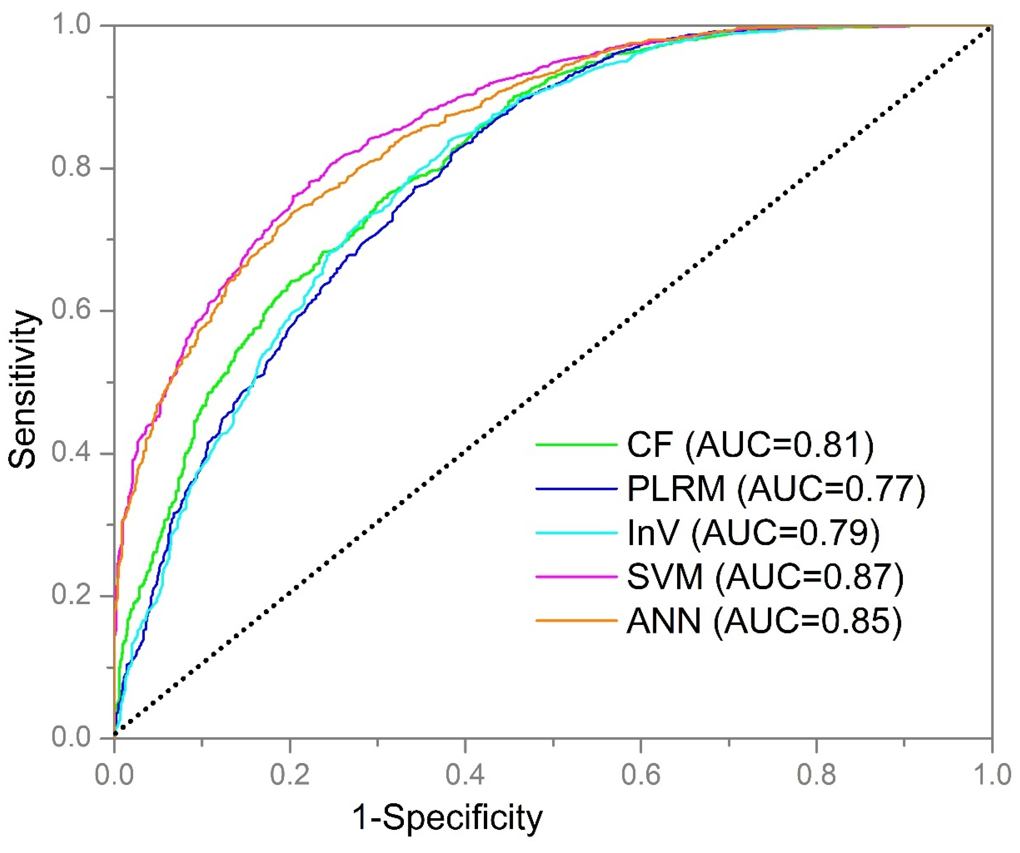
4.6. Model Validation

For the validation process, the total landslides of the entire study area were randomly divided into two groups: training data (5921) and validation data (2538). A ROC plot of sensitivity (true positive rate) and 1-specificity (false positive rate) was made for validation. The prediction rate curves of AUC values of five models (PLFR, InV, CF, ANN and SVM) for validation are 0.77, 0.79, 0.81, 0.85 and 0.87, respectively in Figure 10. According to AUC results, it can be seen that SVM, ANN and CF models (AUC > 0.8) are considered good for application in landslide susceptibility mapping. Additionally, PLFR and InV models (0.7 < AUC < 0.8) are regarded as acceptable. Among these five models, the highest prediction accuracy is the SVM model. Therefore, it can draw a conclusion that the performance of the presented models in this study can satisfy the requirements of landslide prediction.

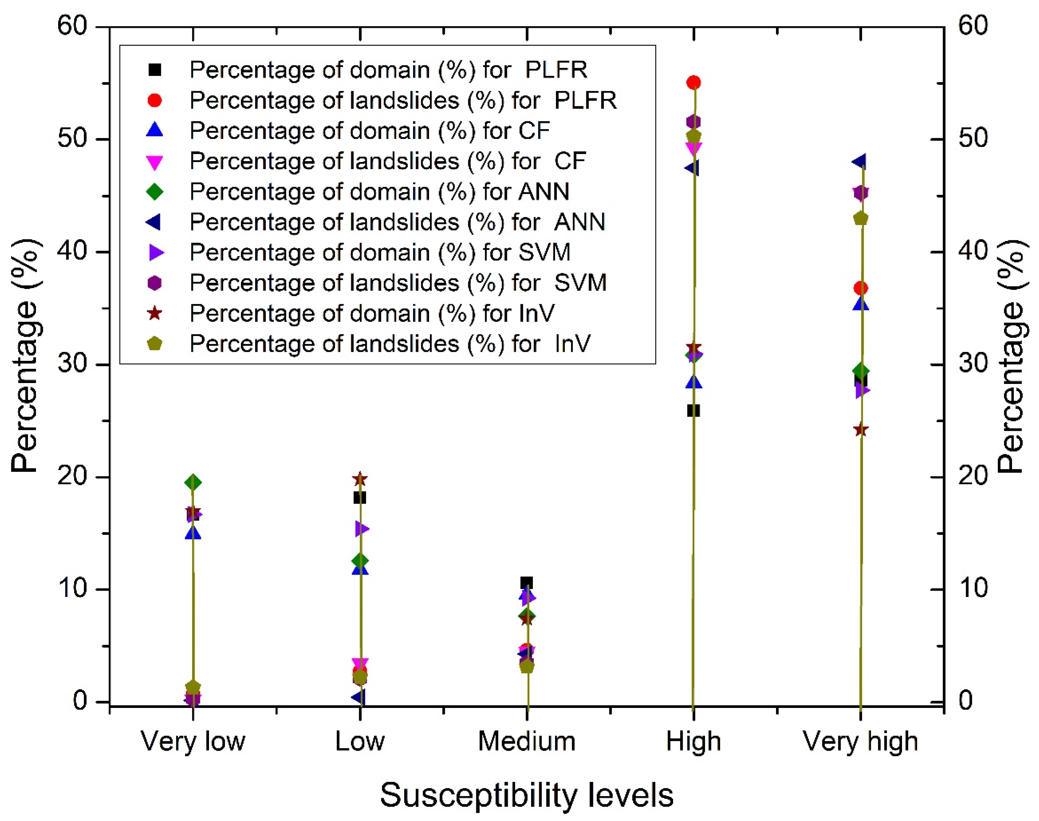
Figure 11 shows that 91.87% of the total landslides occurred in 54.48% of the area classified as high (high and very high) for the PLFR. As for the CF model, 94.52% of the total landslides in 63.67% of the area as high (high and very high). For the InV method, 93.28% accounted for the entire landslides happened in the 55.76% of the area classified from high to very high susceptibility levels. In the case of ANN model, 95.51% of total landslides occurred at 60.26%, while, SVM 96.84% of total landslide occurred in 58.67% of the study area. Among the five models, over 90% landslides occurred in the high area. The above results display that the prediction landslide occurrence of three models agrees with the real condition. From their comparisons, we can see that the most landslides occurred at high and very high susceptible areas of SVM model, while more areas were predicted the susceptible-areas for the CF models, followed by ANN, SVM and PLRM models.

5. Discussion

In recent years, landslide susceptibility studies proposed using various models have been targeted mostly on a single event-type approach. However, in areas such as Japan, massive landslides can be triggered by earthquakes as well as cyclones. In such areas, a single-event approach may not produce high ROC values, but they do not necessarily provide a complete explanation of landslide occurrence due to complex natures of sliding mechanisms. Instead, such models overlook the effect of the type of landslide analyzed. Previously, Chang et al. [42] and Li et al. [69] studied multi-event landslide types for areas in Taiwan and China. However, studies pertaining to the Japanese archipelago is limited to multi-event landslide analysis with the exception of Iwahashi et al. [70] and others [71]. Nevertheless, their studies were focused on landslide characterization rather than a susceptibility modeling approach. This study used landslides triggered by the 2004 Niigata-Chuetsu earthquake and rainfall events in the subsequent period to develop a comprehensive susceptibility model for the region. The models were validated by a mix of both earthquake and rainfall-induced landslides (30%). Despite having given a mixed input, the results returned high ROC values (0.87 and 0.85) indicating the acceptance of SVM and ANN models. More importantly, this study highlights the consideration of slope factor (CF = 1 for class 39°–55°) as an important variable in the Japanese mountainous terrains while modeling the landslide susceptibility. This also confirms the trend noted by Oguchi [72].

Methods for generating LSM maps are numerous based on the GIS platform and many published works discuss to solve the shortages and problems in landslide assessment. The result in this work continues to confirm that the quality of landslide susceptibility assessment is dependent on the method used; where two machine learning models, SVM (AUC = 0.87) and ANN (AUC = 0.85) have clearly better prediction performance than those of the other statistical models. This is because both SVM and ANN have high capacities to deal with non-linear and complex problems as landslides as confirmed in various previous studies [60,73]. In contrast to the SVM model and the ANN model, three statistical models (PLFR, InV and CF) have difficulties to model the complex landslides of the Chuetsu region. This is because these are bivariate models that did not take in the account the complex interactions of the seven causative factors. However, each method has its own unique characteristics and advantages in terms of their ability to include input variables and information provided in temporary stages or the final output that is used to analysis. Such as PLFR-bivariate analyses can help provide a clear understanding of the details of classes in each of the causative factors, which were well reflected in the output maps. The main advantages of CF approach is that CF supplies the advantage of rendering the definition of susceptible classes transparent for the researchers, who are not required to offer a priori the definition of hazard classes but is only charged to interpret a-posteriori the final certainty values and to subdivide the resultant interval into meaningful sub-intervals [33]. For the PLFR model, this is the simplest amongst three models and relatively easy to perform in the ArcGIS platform. 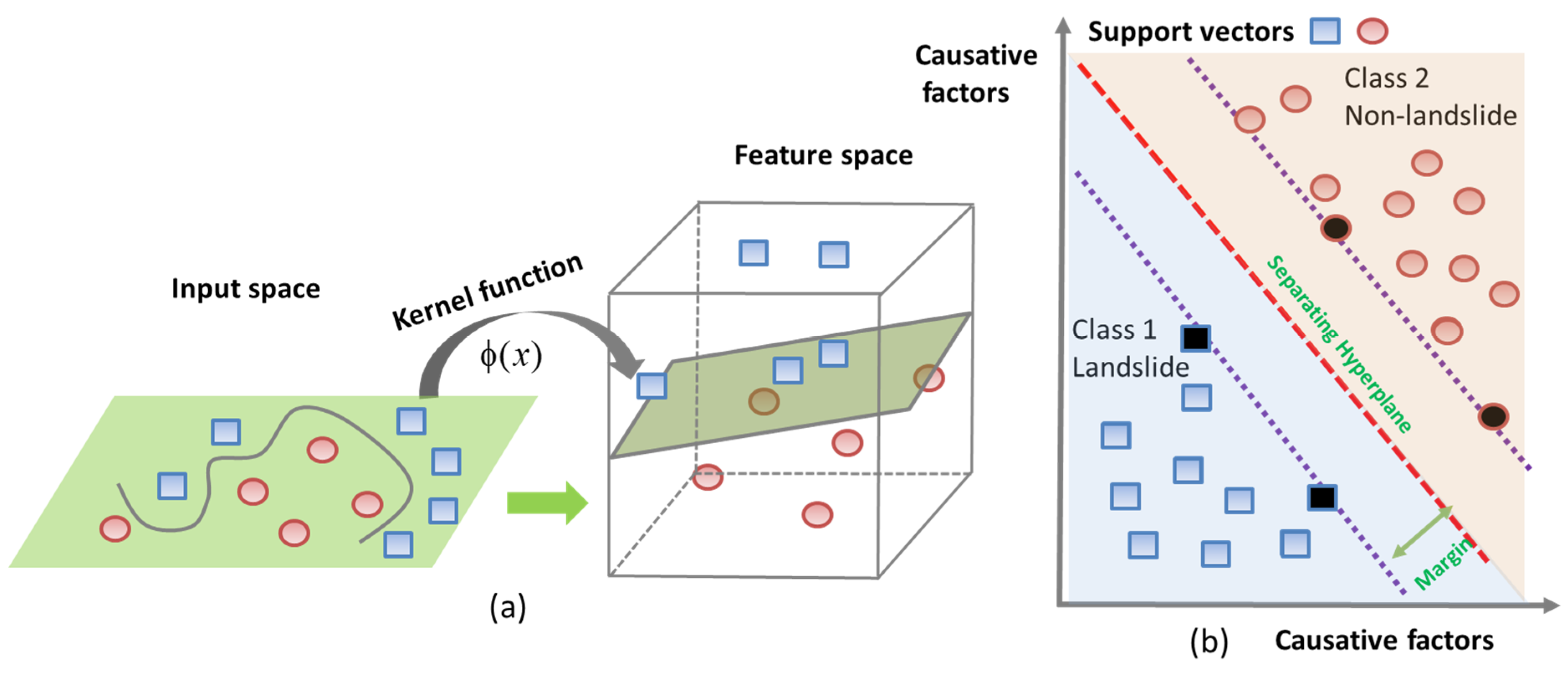The main merits of InV procedures are that the professional, who carries out the analysis, determine the factors combinations of factors used in the evaluation and enable the introduction of expert knowledge into the process [56]. Among the presented three traditional methods, they could provide the details analysis in each class and the results of the relationship between landslide occurrence and causative factors are very similar. The two soft-computing data mining techniques, that is, ANN and SVM, had diverged results. The strength of SVM is ascribed to the accompanying of using a radial basis function (RBF) with the InV values output to create the output map. Additionally, the SVM model is noticeable for processing both the linear and non-linear classification set. The SVM model targets to draw decision boundaries between data support vector points from different class types and separate them with maximal margins [10,23]. To learn the complex functions, SVM uses kernels, while ANN uses multilayer perceptron. The ANN model produced a smooth output with limited details to delineate the hazard zones. The AUC curve plots display that LSM maps produced applying the SVM model is the highest prediction accuracy, followed by the ANN model. CF has the best performance among three traditional statistical models, yet the PLFR model has the lowest accuracy. However, these outcomes indicate that all the models in this study proved reasonably good accuracy in prediction LSM of the Chuetsu area.

Apart from the models what we have compared in this study, there are other more sophisticated approaches are mentioned in the recent literature [74]. Indeed, the comparison of different machine learning models and their performance issues has become a trend in the LSM studies [11,74] However, assessment of model performance not only depends on the methods, but also it is mainly decided by the quality of the collected data [56]. For example, a random forest (RF) model applied using historical 222 landslides in Jiangxi, China with the help of 25 m DEM returned only a ROC value of 0.75 [75]. On a similar note, Dou et al. [34] studied the Osado Island adjoining Niigata using ANN and a 10 m DEM returned a ROC value lower than that achieved for this study. In another example, a case study of the Cameron Highlands, Malaysia using 11 landslide factors and 81 landslide locations by SVM approach achieved maximum accuracy of 0.81 only [76] Thus, the quality of the landslide inventory and high-resolution conditioning factors are important to all statistical models. The current research utilized fine aerial photographs and LiDAR-derived data for conditioning the input variables. This study, regardless of applying multi-event type landslides and traditional machine learning techniques, therefore, achieved a better performance using high-quality dataset.

6. Conclusions

This work carried out a comprehensive assessment of landslides at Chuetsu region in the Niigata Prefecture, Japan. These landslides occurred due to combinations of both earthquake and rainfall-induced events. Based on the results, the following conclusions are offered:

• The high quality of the susceptibility map can be obtained with the use of data mining (SVM and ANN) for landslides triggered by both earthquake and rainfall.
• Although traditional statistical techniques, PLFR, InV and CF, provide low prediction performance of landslide models; however, they are still useful, that is, capacities to reveal high probabilities of the landslide of causative factors’ classes.
• LiDAR-derived data are an important source for deriving high-quality susceptibility map.
• Landslide susceptibility maps developed in this study are of great importance for sustainable urban development and thus the local government. The information derived from the constructed map may be helpful in preliminary decision-making and policy planning. For the hazard zonation, they could opt for some low susceptibility index as a relatively safe area to design the appropriate countermeasures. Furthermore, more relative data are needed to acquire for wide application in more regional areas.

References

1. Marano, K.D.; Wald, D.J.; Allen, T.I. Global earthquake casualties due to secondary effects: A quantitative analysis for improving rapid loss analyses. Nat. Hazards 2010, 319–328. [Google Scholar] [CrossRef]
2. Times, J. 80% of Victims in Atsuma, hardest-Hit by Hokkaido Quake, Died of Suffocation. Available online: https://www.japantimes.co.jp/news/2018/09/11/natio (accessed on 10 December 2018).
3. Turner, A.K.; Schuster, R. Landslides: Investigation and Mitigation; Transportation Research Board: Washington, DC, USA, 1996. [Google Scholar]
4. Camilo, D.C.; Lombardo, L.; Mai, P.M.; Dou, J.; Huser, R. Handling high predictor dimensionality in slope-unit-based landslide susceptibility models through LASSO-penalized Generalized Linear Model. Environ. Model. Softw. 2017, 97, 145–156. [Google Scholar] [CrossRef]
5. Dou, J.; Li, X.; Yunus, A.P.; Paudel, U. Automatic detection of sinkhole collapses at finer resolutions using a multi-component remote sensing approach. Nat. Hazards 2015, 1021–1044. [Google Scholar] [CrossRef]
6. Dou, J.; Yamagishi, H.; Xu, Y.; Zhu, Z.; Yunus, A.P. Characteristics of the Torrential Rainfall-Induced Shallow Landslides by Typhoon Bilis, in July 2006, Using Remote Sensing and GIS. In GIS Landslide; Yamagishi, H., Bhandary, N.P., Eds.; Springer: Tokyo, Japan, 2017; pp. 221–230. ISBN 978-4-431-54391-6. [Google Scholar]
7. Dou, J.; Oguchi, T.; Hayakawa, Y.S.; Uchiyama, S.; Saito, H.; Paudel, U. GIS-based landslide susceptibility mapping using a certainty factor model and its validation in the Chuetsu area, central Japan. In Landslide Science for a Safer Geoenvironment: Volume 2: Methods of Landslide Studies; Springer: Cham, Switzerland, 2014; pp. 419–424. ISBN 9783319050508. [Google Scholar]
8. Chang, K.T.; Dou, J.; Chang, Y.; Kuo, C.P.; Xu, K.M.; Liu, J.K. Spatial resolution effects of digital terrain models on landslide susceptibility analysis. Remote Sens. Spat. Inf. Sci. 2016, XLI-B8, 33–36. [Google Scholar] [CrossRef]
9. Zhu, Z.; Wang, H.; Pang, B.; Dou, J.; Peng, D. Comparison of Conventional Deterministic and Entropy-Based Methods for Predicting Sediment Concentration in Debris Flow. Water 2019, 11, 439. [Google Scholar] [CrossRef]
10. Tien Bui, D.; Pradhan, B.; Lofman, O.; Revhaug, I. Landslide Susceptibility Assessment in Vietnam Using Support Vector Machines, Decision Tree, and Naïve Bayes Models. Math. Probl. Eng. 2012, 2012, 1–26. [Google Scholar] [CrossRef]
11. Dou, J.; Yunus, A.P.; Tien Bui, D.; Merghadi, A.; Sahana, M.; Zhu, Z.; Chen, C.-W.; Khosravi, K.; Yang, Y.; Pham, B.T. Assessment of advanced random forest and decision tree algorithms for modeling rainfall-induced landslide susceptibility in the Izu-Oshima Volcanic Island, Japan. Sci. Total Environ. 2019, 662, 332–346. [Google Scholar] [CrossRef]
12. Tien Bui, D.; Tuan, T.A.; Klempe, H.; Pradhan, B.; Revhaug, I. Spatial prediction models for shallow landslide hazards: A comparative assessment of the efficacy of support vector machines, artificial neural networks, kernel logistic regression, and logistic model tree. Landslides 2016, 13, 361–378. [Google Scholar] [CrossRef]
13. Kanungo, D.P.; Sarkar, S.; Sharma, S. Combining neural network with fuzzy, certainty factor and likelihood ratio concepts for spatial prediction of landslides. Nat. Hazards 2011, 59, 1491–1512. [Google Scholar] [CrossRef]
14. Thai Pham, B.; Prakash, I.; Dou, J.; Singh, S.K.; Trinh, P.T.; Trung Tran, H.; Minh Le, T.; Tran, V.P.; Kim Khoi, D.; Shirzadi, A.; et al. A Novel Hybrid Approach of Landslide Susceptibility Modeling Using Rotation Forest Ensemble and Different Base Classifiers. Geocarto Int. 2018, 1–38. [Google Scholar] [CrossRef]
15. Aleotti, P.; Chowdhury, R. Landslide hazard assessment: Summary review and new perspectives. Bull. Eng. Geol. Environ. 1999, 58, 21–44. [Google Scholar] [CrossRef]
16. Dadson, S.J.; Hovius, N.; Chen, H.; Dade, W.B.; Lin, J.C.; Hsu, M.L.; Lin, C.W.; Horng, M.J.; Chen, T.C.; Milliman, J.; et al. Earthquake-triggered increase in sediment delivery from an active mountain belt. Geology 2004, 32, 733–736. [Google Scholar] [CrossRef]
17. Schlögel, R.; Marchesini, I.; Alvioli, M.; Reichenbach, P.; Rossi, M.; Malet, J.P. Optimizing landslide susceptibility zonation: Effects of DEM spatial resolution and slope unit delineation on logistic regression models. Geomorphology 2018, 301, 10–20. [Google Scholar] [CrossRef]
18. Claessens, L.; Heuvelink, G.; Schoorl, J.M.; Veldkamp, A. DEM resolution effects on shallow landslide hazard and soil redistribution modelling. Earth Surf. Processes Landf. 2005, 30, 461–477. [Google Scholar] [CrossRef]
19. Zhang, W.; Montgomery, D.R. Digital elevation model grid size, landscape representation, and hydrologic simulations. Water Resour. Res. 1994, 30, 1019–1028. [Google Scholar] [CrossRef]
20. Dietrich, W.; Montgomery, D. Scale Dependence and Scale Invariance in Hydrolog; Sposito, G., Ed.; Cambridge University Press: Cambridge, UK, 2008. [Google Scholar]
21. Castellanos Abella, E.A.; Van Westen, C.J. Qualitative landslide susceptibility assessment by multicriteria analysis: A case study from San Antonio del Sur, Guantánamo, Cuba. Geomorphology 2008, 94, 453–466. [Google Scholar] [CrossRef]
22. Jebur, M.N.; Pradhan, B.; Tehrany, M.S. Optimization of landslide conditioning factors using very high-resolution airborne laser scanning (LiDAR) data at catchment scale. Remote Sens. Environ. 2014, 152, 150–165. [Google Scholar] [CrossRef]
23. Dou, J.; Paudel, U.; Oguchi, T.; Uchiyama, S.; Hayakawa, Y.S. Shallow and Deep-Seated Landslide Differentiation Using Support Vector Machines: A Case Study of the Chuetsu Area, Japan. Terr. Atmos. Ocean. Sci. 2015, 26, 227. [Google Scholar] [CrossRef]
24. Jaboyedoff, M.; Choffet, M.; Derron, M.-H.; Horton, P.; Loye, A.; Longchamp, C.; Mazotti, B.; Michoud, C.; Pedrazzini, A. Preliminary Slope Mass Movement Susceptibility Mapping Using DEM and LiDAR DEM. In Terrigenous Mass Movements; Springer Berlin Heidelberg: Berlin, Heidelberg, 2012; ISBN 9783642254956. [Google Scholar]
25. Ghuffar, S.; Szekely, B.; Roncat, A.; Pfeifer, N. Landslide Displacement Monitoring Using 3D Range Flow on Airborne and Terrestrial LiDAR Data. Remote Sens. 2013, 5, 2720–2745. [Google Scholar] [CrossRef]
26. Dou, J.; Qian, J.; Zhang, H.; Chen, S.; Zheng, X.; Zhu, J.; Xie, Z.; Zou, Y. Landslides detection: A case study in Conghua city of Pearl River delta. In Proceedings of the Second International Conference on Earth Observation for Global Changes, Chengdu, China, 25–29 May 2009. [Google Scholar] [CrossRef]
27. Dou, J.; Chang, K.T.; Chen, S.; Yunus, A.P.; Liu, J.K.; Xia, H.; Zhu, Z. Automatic Case-Based Reasoning Approach for Landslide Detection: Integration of Object-Oriented Image Analysis and a Genetic Algorithm. Remote Sens. 2015, 7, 4318–4342. [Google Scholar] [CrossRef]
28. Bijukchhen, S.M.; Kayastha, P.; Dhital, M.R. A comparative evaluation of heuristic and bivariate statistical modelling for landslide susceptibility mappings in Ghurmi-Dhad Khola, east Nepal. Arab. J. Geosci. 2013, 6, 2727–2743. [Google Scholar] [CrossRef]
29. Guzzetti, F.; Carrara, A.; Cardinali, M.; Reichenbach, P. Landslide hazard evaluation: A review of current techniques and their application in a multi-scale study, central Italy. Geomorphology 1999, 31, 181–216. [Google Scholar] [CrossRef]
30. De Vita, P.; Napolitano, E.; Godt, J.W.; Baum, R.L. Deterministic estimation of hydrological thresholds for shallow landslide initiation and slope stability models: Case study from the Somma-Vesuvius area of southern Italy. Landslides 2013, 10, 713–728. [Google Scholar] [CrossRef]
31. Shahabi, H.; Ahmad, B.B.; Khezri, S. Evaluation and comparison of bivariate and multivariate statistical methods for landslide susceptibility mapping (case study: Zab basin). Arab. J. Geosci. 2013, 6, 3885–3907. [Google Scholar] [CrossRef]
32. Dou, J.; Bui, D.T.; Yunus, A.P.; Jia, K.; Song, X.; Revhaug, I.; Xia, H.; Zhu, Z. Optimization of causative factors for landslide susceptibility evaluation using remote sensing and GIS data in parts of Niigata, Japan. PLoS ONE 2015, 10, e0133262. [Google Scholar] [CrossRef] [PubMed]
33. Binaghi, E.; Luzi, L.; Madella, P.; Pergalani, F.; Rampini, A. Slope Instability Zonation: A Comparison Between Certainty Factor and Fuzzy Dempster–Shafer Approaches. Nat. Hazards 1998, 17, 77–97. [Google Scholar] [CrossRef]
34. Dou, J.; Yamagishi, H.; Pourghasemi, H.R.; Yunus, A.P.; Song, X.; Xu, Y.; Zhu, Z. An integrated artificial neural network model for the landslide susceptibility assessment of Osado Island, Japan. Nat. Hazards 2015, 78, 1749–1776. [Google Scholar] [CrossRef]
35. Collins, B.D.; Kayen, R.; Tanaka, Y. Spatial distribution of landslides triggered from the 2007 Niigata Chuetsu–Oki Japan Earthquake. Eng. Geol. 2012, 127, 14–26. [Google Scholar] [CrossRef]
36. Has, B.; Nozaki, T. Role of geological structure in the occurrence of earthquake-induced landslides, the case of the 2007 Mid-Niigata Offshore Earthquake, Japan. Eng. Geol. 2014, 182, 25–36. [Google Scholar] [CrossRef]
37. Yamagishi, H.; Marui, H.; Ayalew, L.; Sekiguchi, T.; Horimatsu, T.; Hatamoto, M. Estimation of the sequence and size of the Tozawagawa landslide, Niigata, Japan, using aerial photographs. Landslides 2004, 1, 299–303. [Google Scholar] [CrossRef]
38. Takeuchi, K.; Yanagisawa, Y. 1:50,000 Digital Geological Map of the Uonuma Region, Niigata Prefecture (Ver. 1); Geological Survey of Japan: Tsukuba, Japan, 2004; Volume V20B-2. [Google Scholar]
39. Varnes, D.J. Slope movement types and processes, in Schuster, R.L., and Krizek, R.J., eds., Landslides—Analysis and control. Natl. Acad. Sci. Transp. Res. Board Spec. Rep. 1978, 176, 11–33. [Google Scholar]
40. Aksoy, B.; Ercanoglu, M. Landslide identification and classification by object-based image analysis and fuzzy logic: An example from the Azdavay region (Kastamonu, Turkey). Comput. Geosci. 2012, 38, 87–98. [Google Scholar] [CrossRef]
41. Xu, C.; Ma, S.; Tan, Z.; Xie, C.; Toda, S.; Huang, X. Landslides triggered by the 2016 Mj 7. 3 Kumamoto, Japan, earthquake. Landslide 2018, 26, 551–564. [Google Scholar] [CrossRef]
42. Chang, K.-T.; Chiang, S.-H.; Hsu, M.-L. Modeling typhoon- and earthquake-induced landslides in a mountainous watershed using logistic regression. Geomorphology 2007, 89, 335–347. [Google Scholar] [CrossRef]
43. García-Rodríguez, M.J.; Malpica, J.A. Assessment of earthquake-triggered landslide susceptibility in El Salvador based on an artificial neural network model. Nat. Hazards Earth Syst. Sci. 2010, 10, 1307–1315. [Google Scholar] [CrossRef]
44. Bhandary, N.P.; Dahal, R.K.; Timilsina, M.; Yatabe, R. Rainfall event-based landslide susceptibility zonation mapping. Natural Hazards 2013, 69, 365–388. [Google Scholar] [CrossRef]
45. Conforti, M.; Pascale, S.; Robustelli, G.; Sdao, F. Evaluation of prediction capability of the artificial neural networks for mapping landslide susceptibility in the Turbolo River catchment (northern Calabria, Italy). Catena 2014, 113, 236–250. [Google Scholar] [CrossRef]
46. Tanyaş, H.; Allstadt, K.E.; van Westen, C.J. An updated method for estimating landslide-event magnitude. Earth Surf. Processes Landf. 2018, 43, 1836–1847. [Google Scholar] [CrossRef]
47. Youssef, A.M.; Pradhan, B.; Jebur, M.N.; El-Harbi, H.M. Landslide susceptibility mapping using ensemble bivariate and multivariate statistical models in Fayfa area, Saudi Arabia. Environ. Earth Sci. 2015, 73, 3745–3761. [Google Scholar] [CrossRef]
48. Peckham, S.D. Profile, plan and streamline curvature: A simple derivation and applications. In Proceedings of the Geomorphometry, Redlands, CA,USA, 7–11 September 2011; 2011; Volume 4, pp. 27–30. [Google Scholar]
49. Ohlmacher, G.C. Plan curvature and landslide probability in regions dominated by earth flows and earth slides. Eng. Geol. 2007, 91, 117–134. [Google Scholar] [CrossRef]
50. Lin, W.T.; Chou, W.C.; Lin, C.Y.; Huang, P.H.; Tsai, J.S. Automated suitable drainage network extraction from digital elevation models in Taiwan’s upstream watersheds. Hydrol. Processes 2006, 20, 289–306. [Google Scholar] [CrossRef]
51. Hayakawa, Y.S.; Oguchi, T. GIS analysis of fluvial knickzone distribution in Japanese mountain watersheds. Geomorphology 2009. [Google Scholar] [CrossRef]
52. Oguchi, T. Drainage density and relative relief in humid steep mountains with frequent slope failure. Earth Surf. Processes Landf. 1997, 22, 107–120. [Google Scholar] [CrossRef]
53. Kawabata, D.; Bandibas, J. Landslide susceptibility mapping using geological data, a DEM from ASTER images and an Artificial Neural Network (ANN). Geomorphology 2009, 113, 97–109. [Google Scholar] [CrossRef]
54. Yalcin, A.; Reis, S.; Aydinoglu, A.C.; Yomralioglu, T. A GIS-based comparative study of frequency ratio, analytical hierarchy process, bivariate statistics and logistics regression methods for landslide susceptibility mapping in Trabzon, NE Turkey. Catena 2011, 85, 274–287. [Google Scholar] [CrossRef]
55. Pradhan, B.; Lee, S. Landslide susceptibility assessment and factor effect analysis: Backpropagation artificial neural networks and their comparison with frequency ratio and bivariate logistic regression modelling. Environ. Model. Softw. 2010, 25, 747–759. [Google Scholar] [CrossRef]
56. Van Westen, C.J.; Asch, T.W.J.; Soeters, R.; Westen, C.J. Landslide hazard and risk zonation—Why is it still so difficult? Bull. Eng. Geol. Environ. 2005, 65, 167–184. [Google Scholar] [CrossRef]
57. Chung, C.-J.; Fabbri, A.G. The representation of geoscience information for data integration. Nonrenew. Resour. 1993, 2, 122–139. [Google Scholar] [CrossRef]
58. Ostad-Ali-Askari, K.; Shayannejad, M.; Ghorbanizadeh-Kharazi, H. Artificial neural network for modeling nitrate pollution of groundwater in marginal area of Zayandeh-rood River, Isfahan, Iran. KSCE J. Civ. Eng. 2017. [Google Scholar] [CrossRef]
59. Khosravi, A.; Koury, R.N.N.; Machado, L.; Pabon, J.J.G. Prediction of wind speed and wind direction using artificial neural network, support vector regression and adaptive neuro-fuzzy inference system. Sustain. Energy Technol. Assess. 2018. [Google Scholar] [CrossRef]
60. Dou, J.; Yamagishi, H.; Zhu, Z.; Yunus, A.P.; Chen, C.W. A Comparative Study of the Binary Logistic Regression (BLR) and Artificial Neural Network (ANN) Models for GIS-Based Spatial Predicting Landslides at a Regional Scale. In Landslide Dynamics: ISDR-ICL Landslide Interactive Teaching Tools: Volume 1: Fundamentals, Mapping and Monitoring; Springer: Cham, Switzerland, 2018; pp. 139–151. ISBN 978-3-319-53486-2. [Google Scholar]
61. Pham, B.T.; Tien Bui, D.; Prakash, I.; Dholakia, M.B. Hybrid integration of Multilayer Perceptron Neural Networks and machine learning ensembles for landslide susceptibility assessment at Himalayan area (India) using GIS. Catena 2017. [Google Scholar] [CrossRef]
62. Vapnik, V.N. Statistical Learning Theory (Adaptive and Learning Systems for Signal Processing, Communications and Control Series); Wiley-Interscience: Hoboken, NJ, USA, 1998; ISBN 0471030031. [Google Scholar]
63. Su, C.; Wang, L.; Wang, X.; Huang, Z.; Zhang, X. Mapping of rainfall-induced landslide susceptibility in Wencheng, China, using support vector machine. Nat. Hazards 2015, 76, 1759–1779. [Google Scholar] [CrossRef]
64. Zhu, Z.; Wang, H.; Peng, D.; Dou, J. Modelling the Hindered Settling Velocity of a Falling Particle in a Particle-Fluid Mixture by the Tsallis Entropy Theory. Entropy 2019, 21, 55. [Google Scholar] [CrossRef]
65. Irigaray, C.; Fernández, T.; El Hamdouni, R.; Chacón, J. Evaluation and validation of landslide-susceptibility maps obtained by a GIS matrix method: Examples from the Betic Cordillera (southern Spain). Nat. Hazards 2006, 41, 61–79. [Google Scholar] [CrossRef]
66. Swets, J.A. Measuring the accuracy of diagnostic systems. Science 1988, 240, 1285–1293. [Google Scholar] [CrossRef]
67. Yesilnacar, E.; Topal, T. Landslide susceptibility mapping: A comparison of logistic regression and neural networks methods in a medium scale study, Hendek region (Turkey). Eng. Geol. 2005, 79, 251–266. [Google Scholar] [CrossRef]
68. Yilmaz, I. Landslide susceptibility mapping using frequency ratio, logistic regression, artificial neural networks and their comparison: A case study from Kat landslides (Tokat—Turkey). Comput. Geosci. 2009, 35, 1125–1138. [Google Scholar] [CrossRef]
69. Li, Y.; Chen, G.; Tang, C.; Zhou, G.; Zheng, L. Rainfall and earthquake-induced landslide susceptibility assessment using GIS and Artificial Neural Network. Nat. Hazards Earth Syst. Sci. 2012, 12, 2719–2729. [Google Scholar] [CrossRef]
70. Iwahashi, J.; Kamiya, I.; Yamagishi, H. High-resolution DEMs in the study of rainfall- and earthquake-induced landslides: Use of a variable window size method in digital terrain analysis. Geomorphology 2012, 153, 29–38. [Google Scholar] [CrossRef]
71. Saito, H.; Uchiyama, S.; Hayakawa, Y.S.; Obanawa, H. Landslides triggered by an earthquake and heavy rainfalls at Aso volcano, Japan, detected by UAS and SfM-MVS photogrammetry. Progr. Earth Planet. Sci. 2018. [Google Scholar] [CrossRef]
72. Oguchi, T. Factors affecting the magnitude of post-glacial hillslope incision in Japanese mountains. Catena 1996, 26, 171–186. [Google Scholar] [CrossRef]
73. Merghadi, A.; Abderrahmane, B.; Tien Bui, D. Landslide Susceptibility Assessment at Mila Basin (Algeria): A Comparative Assessment of Prediction Capability of Advanced Machine Learning Methods. ISPRS Int. J. Geo-Inf. 2018, 7, 268. [Google Scholar] [CrossRef]
74. Reichenbach, P.; Rossi, M.; Malamud, B.D.; Mihir, M.; Guzzetti, F. A review of statistically-based landslide susceptibility models. Earth-Sci. Rev. 2018, 180, 60–91. [Google Scholar] [CrossRef]
75. Chen, W.; Peng, J.; Hong, H.; Shahabi, H.; Pradhan, B.; Liu, J.; Zhu, A.X.; Pei, X.; Duan, Z. Landslide susceptibility modelling using GIS-based machine learning techniques for Chongren County, Jiangxi Province, China. Sci. Total Environ. 2018, 626, 1121–1135. [Google Scholar] [CrossRef]
76. Pradhan, B.; Sameen, M.I. Manifestation of SVM-Based Rectified Linear Unit (ReLU) Kernel Function in Landslide Modelling. In Space Science and Communication for Sustainability; Springer Singapore: Singapore, 2018; pp. 185–195. [Google Scholar]
Figure 1. (a) Location of Japan; (b) landslide distribution, randomly divided into two sets: training and testing.
Remotesensing 11 00638 g001
Figure 2. Illustrating the characteristics and different types of landslides in the study area: (a) shallow spread in the north of the Hitotsuminesawa with water, Nagaoka city; (b) rotational soil slide in north of Mushigame; (c) bedrock collapse severely destroyed the road in Nagaoka; (d) translational slide, an arrow display secondary scarp in the Uonuma city (Images provided by NIED).
Remotesensing 11 00638 g002
Figure 3. Framework for landslide susceptibility mapping (LSM) maps in the study.
Remotesensing 11 00638 g003
Figure 4. Probability of density distribution for landslide area.
Remotesensing 11 00638 g004
Figure 5. Landslide causative factors maps in this study: (a) elevation, (b) slope angle, (c) slope aspect, (d) plan curvature, (e) drainage density, (f) density of geologic boundaries, (g) lithology.
Remotesensing 11 00638 g005
Figure 6. Structure of a three-layer of neural networks for landslide susceptibility analysis.
Remotesensing 11 00638 g006
Figure 7. Illustration of support vector machine (SVM) principle: (a) Input space is mapped to the feature space with the help of a kernel function; (b) Separating hyperplane and margin for landslide classification.
Remotesensing 11 00638 g007
Figure 8. Number of hidden neurons impacts the ANN network: Coefficient of determination R2 has the largest value (0.96) when the number of hidden neurons is 11.
Remotesensing 11 00638 g008
Figure 9. LSM maps produced by (a) PLFR, (b) InV, (c) CF, (d) ANN and (e) SVM models, respectively.
Remotesensing 11 00638 g009
Figure 10. Validation for the performance of five models applying ROC curve in this study.
Remotesensing 11 00638 g010
Figure 11. Comparison of the relative distribution of susceptibility levels using PLFR, InV, CF, ANN and SVM models, respectively.
Remotesensing 11 00638 g011