Long-Term Variations in the Pixel-to-Pixel Variability of NOAA AVHRR SST Fields from 1982 to 2015


1
Department of Marine Technology, College of Information Science and Engineering, Ocean University of China, 238 Songling Road, Qingdao 266100, China
2
Graduate School of Oceanography, University of Rhode Island, 215 South Ferry Road, Narragansett, RI 02882, USA
3
Qian Xuesen Laboratory of Space Technology, China Academy of Space Technology, 104 Youyi Road, Beijing 100094, China
4
Laboratory for Regional Oceanography and Numerical Modeling, Qingdao National Laboratory for Marine Science and Technology, 1 Wenhai Road, Qingdao 266237, China
5
Rosenstiel School of Marine and Atmospheric Science, University of Miami, 4600 Rickenbacker Causeway, Miami, FL 33149-1031, USA
*
Author to whom correspondence should be addressed.
Remote Sens. 2019, 11(7), 844; https://0-doi-org.brum.beds.ac.uk/10.3390/rs11070844
Submission received: 24 February 2019
/
Revised: 25 March 2019
/
Accepted: 30 March 2019
/
Published: 8 April 2019
(This article belongs to the Section Ocean Remote Sensing)
Abstract
:Sea surface temperature (SST) fields obtained from the series of space-borne five-channel Advanced Very High Resolution Radiometers (AVHRRs) provide the longest continuous time series of global SST available to date (1981–present). As a result, these data have been used for many studies and significant effort has been devoted to their careful calibration in an effort to provide a climate quality data record. However, little attention has been given to the local precision of the SST retrievals obtained from these instruments, which we refer to as the pixel-to-pixel (p2p) variability, a characteristic important in the ability to resolve structures such as ocean fronts characterized by small gradients in the SST field. In this study, the p2p variability is estimated for Level-2 SST fields obtained with the Pathfinder retrieval algorithm for AVHRRs on NOAA-07, 9, 11, 12 and 14-19. These estimates are stratified by year, season, day/night and along-scan/along-track. The overall variability ranges from 0.10 K to 0.21 K. For each satellite, the along-scan variability is between 10 and 20% smaller than the along-track variability (except for NOAA-16 nighttime for which it is approximately 30% smaller) and the summer and fall s are between 10 and 15% smaller than the winter and spring s. The differences between along-track and along-scan are attributed to the way in which the instrument has been calibrated. The seasonal differences result from the term in the Pathfinder retrieval algorithm. This term is shown to be a major contributor to the p2p variability and it is shown that its impact could be substantially reduced without a deleterious effect on the overall p2p of the resulting products by spatially averaging it as part of the retrieval process. The AVHRR/3s (NOAA-15 through 19) were found to be relatively stable with trends in the p2p variability of at most 0.015 K/decade.

1. Introduction
Wu et al. [1] (Wu2017 hereafter) examined two approaches to estimating the spatial precision of sea surface temperature (SST) fields obtained from satellite-borne infrared radiometers, one based on the spectral characteristics of the data and the other on their spatial characteristics. They defined the spatial precision as the scatter of an SST field over a small region (defined by a length scale of km or less) after removal of the local geophysical variability. However, following publication of Wu2017, concern was raised within the Group for High Resolution Sea Surface Temperature (GHRSST) with regard to the use of the expression spatial precision; from several perspectives the expression was found to be confusing. We have therefore decided, following discussion with several GHRSST Science Team members, to use pixel-to-pixel variability, which we abbreviate as p2p , in place of spatial precision in the following. The expression spatial precision (p2p ) was used to differentiate the local scatter of SST retrievals from the scatter of satellite-derived SST retrievals compared with in situ temperature observations (satellite-in situ match-ups). A significant contribution to the scatter determined from the match-ups comes from long wavelength variations in the atmosphere, which are not fully accounted for by the retrieval algorithm. Because this contribution to the error is long wavelength, it does not contribute to the scatter over small spatial scales.
To demonstrate the two methods, Wu2017 estimated the p2p of Level-2 (L2 [2]) SST fields obtained from the Advanced Very High Resolution Radiometer (AVHRR) on NOAA-15 and from the Visible-Infrared Imager-Radiometer Suite (VIIRS) on Suomi-NPP (National Polar-orbiting Partnership). Based on a White Paper prepared by the NASA-NOAA SST Science Team, addressing issues related to the SST error budget [3], Wu2017 argued that misclassification of cloud-contaminated pixels, normally associated with retrieval errors, in addition to instrument noise contributes to the p2p . Assuming that misclassification errors increase with fractional cloud cover, Wu2017 minimized the contribution of misclassified pixels in their estimates of the p2p by considering only regions that were sufficiently cloud free to allow them to fill gaps, resulting from clouds, without affecting the statistics of the fields. This means that their estimates of p2p relate only to the noise associated with the instruments and their calibration, and how this noise propagates through the retrieval algorithm; their estimates do not include errors in the retrievals associated with uncorrected atmospheric effects or cloud-contaminated pixels flagged as clear. Important for the work presented herein, the work of Wu2017 showed that the two approaches, spectral and spatial, provided very nearly the same estimates of p2p for AVHRR on NOAA-15, between 0.15 and 0.2 K.
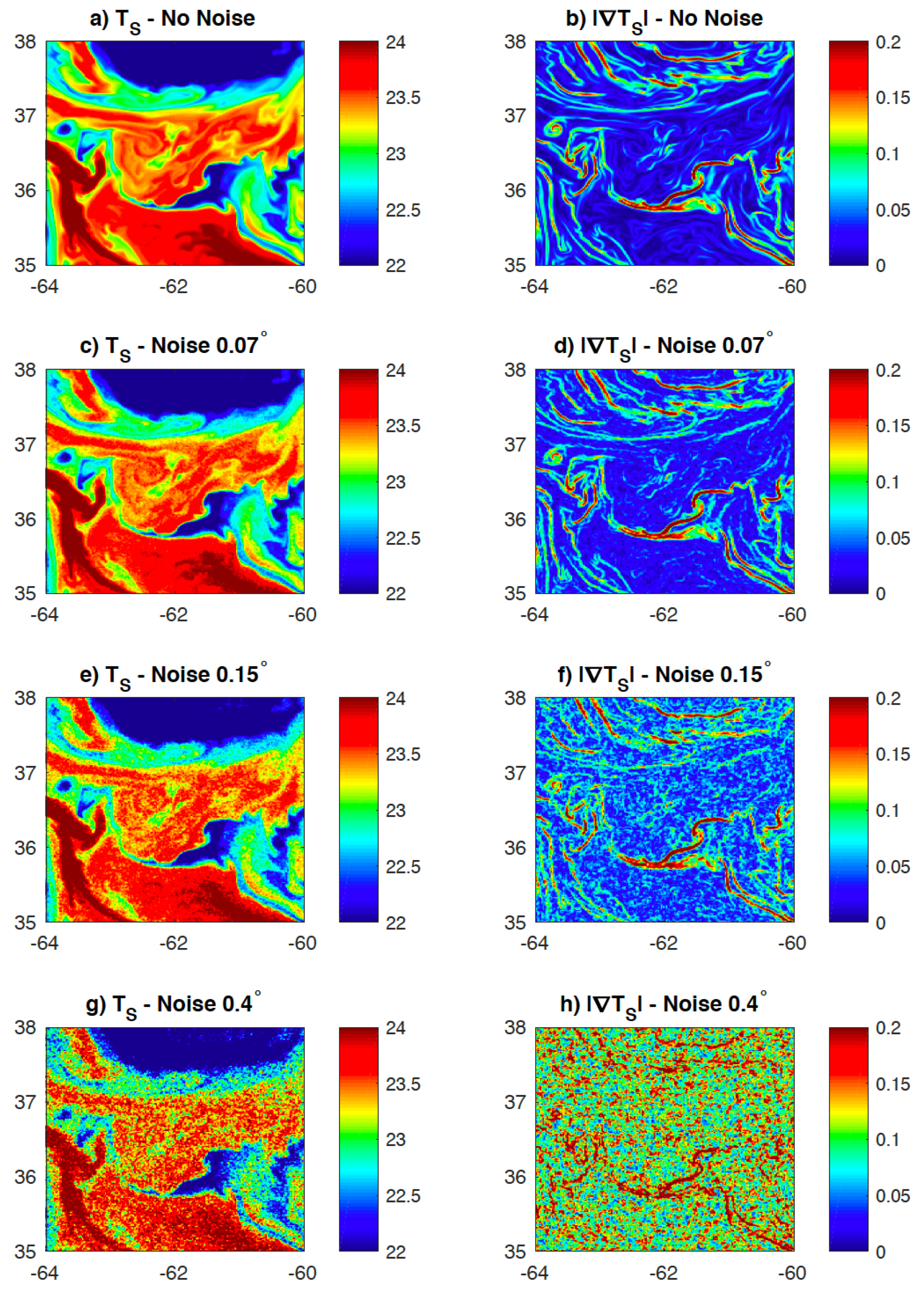
Why the interest in p2p when the accuracy of the retrievals based on satellite-in situ matchups is already known? Wu2017 examined the impact of p2p on the gradient of SST fields noting, in particular, that errors in the SST field result in a bias in the SST gradient magnitude, which is a function of p2p . Given the interest in recent studies in trends in the gradient magnitude [4,5] and the significant difference between the standard deviation of the satellite-in situ matchups and the p2p values Wu2017 obtained for NOAA-15, it is clear that better documentation of within-instrument trends and/or inter-instrument differences in the p2p is of importance. Another way to appreciate the importance of p2p is to examine the difference between gradient fields obtained from SST fields with different levels of noise. Figure 1a shows a small region of the SST field at the edge of the Gulf Stream extracted from the LLC-4320 simulation, a global simulation of the ocean with 90 vertical levels and a spatial resolution of 2 km [6,7]. Figure 1b shows the gradient magnitude of the field shown in Figure 1a. Subsequent rows in the figure show the same SST field, with the addition of Gaussian noise, and the associated gradient magnitude field. All but the strongest gradients are lost in the noise of the gradient magnitude field obtained from the original field plus noise equivalent to that determined from the satellite-in situ matchups, 0.4 K (Figure 1g,h). The finer structure evident in the gradient of the original field (Figure 1b), is also lost in the gradient field obtained from the original field plus noise equivalent to that of the AVHRR p2p but much of the rest of the structure is still visible (Figure 1e,f). By contrast, most of the fine scale structure remains in the gradient of the SST field with noise corresponding to the VIIRS p2p , (Figure 1d). Given that the accuracy of SST fields obtained from most satellite-borne radiometers ranges from 0.3 to 0.4 K while the p2p of the same SST fields ranges from 0.05 to 0.2 K, knowledge of the p2p is critical when selecting the data to use for studies involving SST gradients.
In light of the above, we undertook the task of determining the p2p attributable to instrument and calibration noise for all five-channel AVHRR sensors carried on NOAA polar-orbiting spacecraft from NOAA-07 (launched in October 1981) through NOAA-19 (launched in February 2009). The ultimate objective of this work was to document temporal trends in the p2p as well as inter-instrument differences in this regard. Our estimates of the p2p are based on the spectral approach introduced in Wu2017.
2. Data
This study uses the full resolution (nominally 1.1 km) AVHRR SST product derived with the Pathfinder retrieval algorithm developed at the University of Miami [8]. Retrievals were performed at the University of Rhode Island (URI). The algorithm was applied to the High Resolution Picture Transmission (HRPT) data stream obtained from the AVHRR/2 instruments on NOAA-07, 9, 11, 12 and14 and the AVHRR/3 instruments on NOAA-15 through NOAA-19. The raw data were downloaded from the satellites at the Wallops Island, VA, USA receiving station and archived in NOAA’s Comprehensive Large Array-data Stewardship System (CLASS), from which they were obtained. The period covered by the data used herein extends from January 1982 through May 2015, but the coverage in time is quite erratic as will be shown in the next section.
The University of Miami retrieval algorithm (described in a bit more detail in Section 5.1 and referred to as the Pathfinder retrieval algorithm hereafter) is capable of producing both L2 and, from these, L3 SST fields. We chose to use the L2 AVHRR SST product because these fields do not include the pixel-to-pixel variability introduced by interpolation and other processes in data gridding that are common to the L3 fields. We also used only pixels with a quality level of 3 or higher, again to allow us to isolate instrument noise and line-to-line calibration issues from other factors contributing to the noise in the SST fields.
The nominal pixel spacing in the along-scan direction is 1.1 km, but it increases from approximately 750 m at nadir to over 4 km on the swath edge, while the along-track pixel spacing varies by less than 1% about the nominal value of 1.1 km with distance from nadir [1]. Because the spectral method ensemble averages spectra, hence is sensitive to pixel spacing, only temperature sections lying within 500 km of nadir, of the approximately 2800 km scan, were used in this study, resulting in the largest values of the spacing being less than 1.6 km.
We used the same region in the Sargasso Sea, 63–72W, 32–36N used by Wu2017. This region was initially chosen because it included in situ data from the MV Oleander, used by Wu2017 to validate the method because the region is well covered by the data acquired at Wallops Island and because the region is dynamically quiet; i.e., the geophysical variability does not overwhelm the sensor noise as it might in more dynamically active regions. The latter turns out not to be an issue for SST fields obtained from AVHRR radiances. In fact, if the region is too quiet dynamically, the p2p is underestimated by the spectral approach as will be shown below.
3. Processing
The spectral approach used to determine the p2p of the various instruments is based on the spatial power spectrum of temperature sections extracted from the SST fields. The slope of the spatial power spectral density (PSD) of noise-free SST sections in the study area, i.e., the PSD due to geophysical variability, is very nearly linear (in log–log space) from several hundred meters to more than 100 km [1]. Deviation from this linearity at small spatial scales (large wavenumbers) is due to noise in the retrieved SST field introduced either by noise in the instrument, the calibration process or the retrieval process. The least squares best fit (in log–log space) of the observed PSD to a simulated PSD, assuming a linear geophysical spectrum and white noise, was used to determine the level of noise in spectral space:
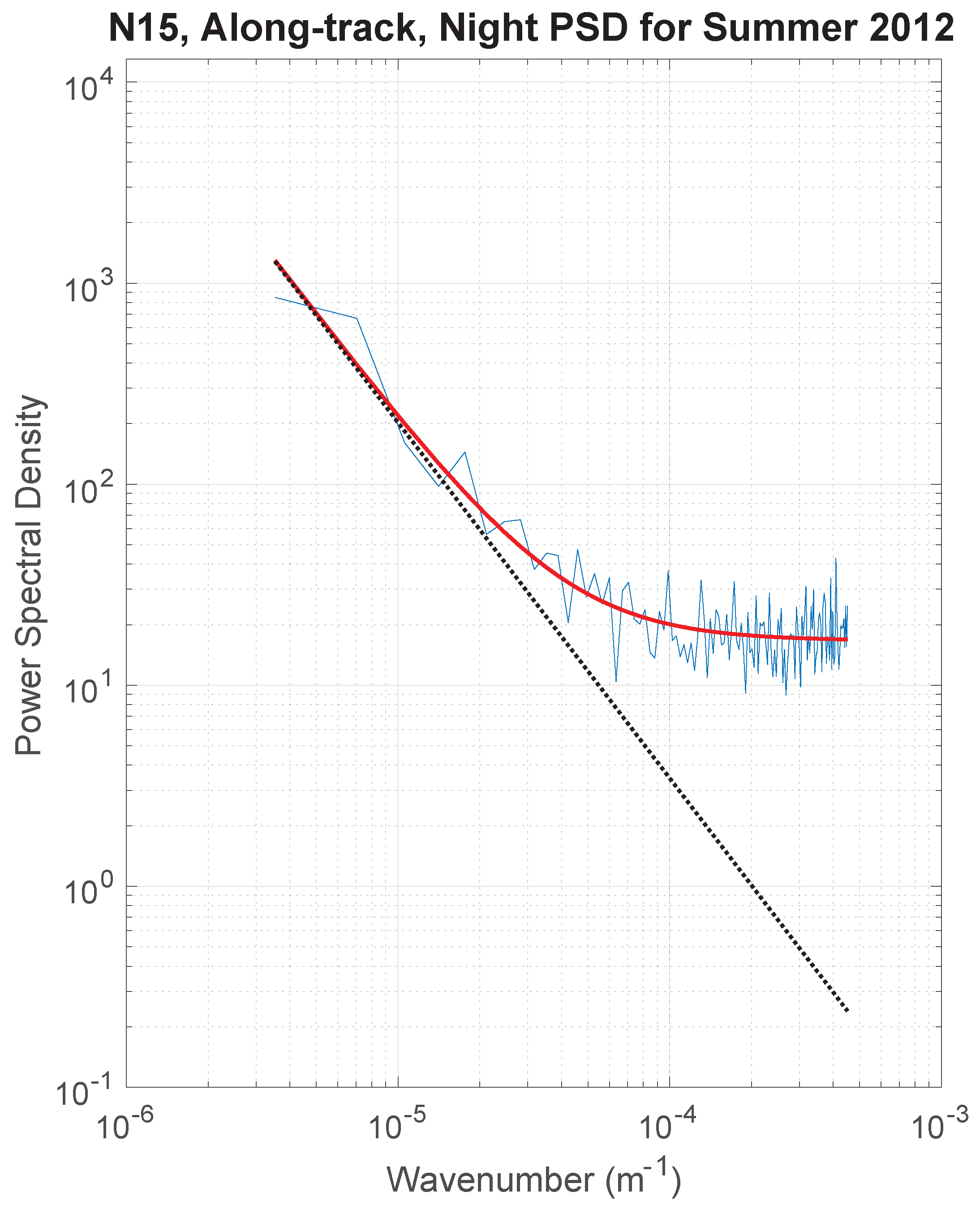
where slope and intercept define the straight line portion of the best fit spectrum in log–log space, noise is the noise level also in spectral space, is the wavenumber of the spectral component and PSD the corresponding power spectral density of the satellite spectrum. Figure 2 is an example of such a fit. Noise in the original temperature spectrum was determined from the spectral noise via a second simulation described later in this section.
In order to separate the noise from the geophysical variability, the length of the temperature sections used for the analysis must be sufficiently long that the linear decay of the spectra (in log–log space) due to geophysical variability in the SST field can be determined. However, the longer the sections, the more likely they are to include gaps due to clouds—the PSD were calculated by the Fast Fourier Transform (FFT), which requires that the sections have no missing samples and that the samples on the sections be equally spaced. Based on these considerations, we selected non-overlapping 256 pixel long temperature sections, which vary in length from approximately 200 to 400 km. (The range of length is due to the difference in pixel spacing discussed in Section 2. The bulk of the variability is in the along-scan length; the along-track lengths ranged from 280 to 286 km.) Sections were selected in the along-scan and along-track (across-scan) directions. Selection of sections was constrained by the number of cloud free pixels on and in the vicinity of the section—in order to allow proper gap filling and to reduce the number of misclassified pixels (cloud contaminated pixels flagged as clear) along the section.
Requiring that all 256 pixels on a given section be cloud-free resulted in a dataset that is too small for the analyses described herein. In order to (significantly) increase the number of useable sections, we began with sections that were at least 90% clear and then followed the approach of Wu2017 to fill gaps. The mean spacing on each section was then determined and the data were nearest-neighbor resampled to points starting with the first value and continuing at the mean spacing for 256 points. Each section was then detrended and FFTed. No filtering, beyond the detrending, was applied to the sections in that standard filters were found to affect the high wavenumber end of the spectrum from which the noise was determined. The PSD was determined from the FFT and then nearest-neighbor interpolated to a fixed wavenumber vector, allowing for the combination of spectra in the subsequent analysis.
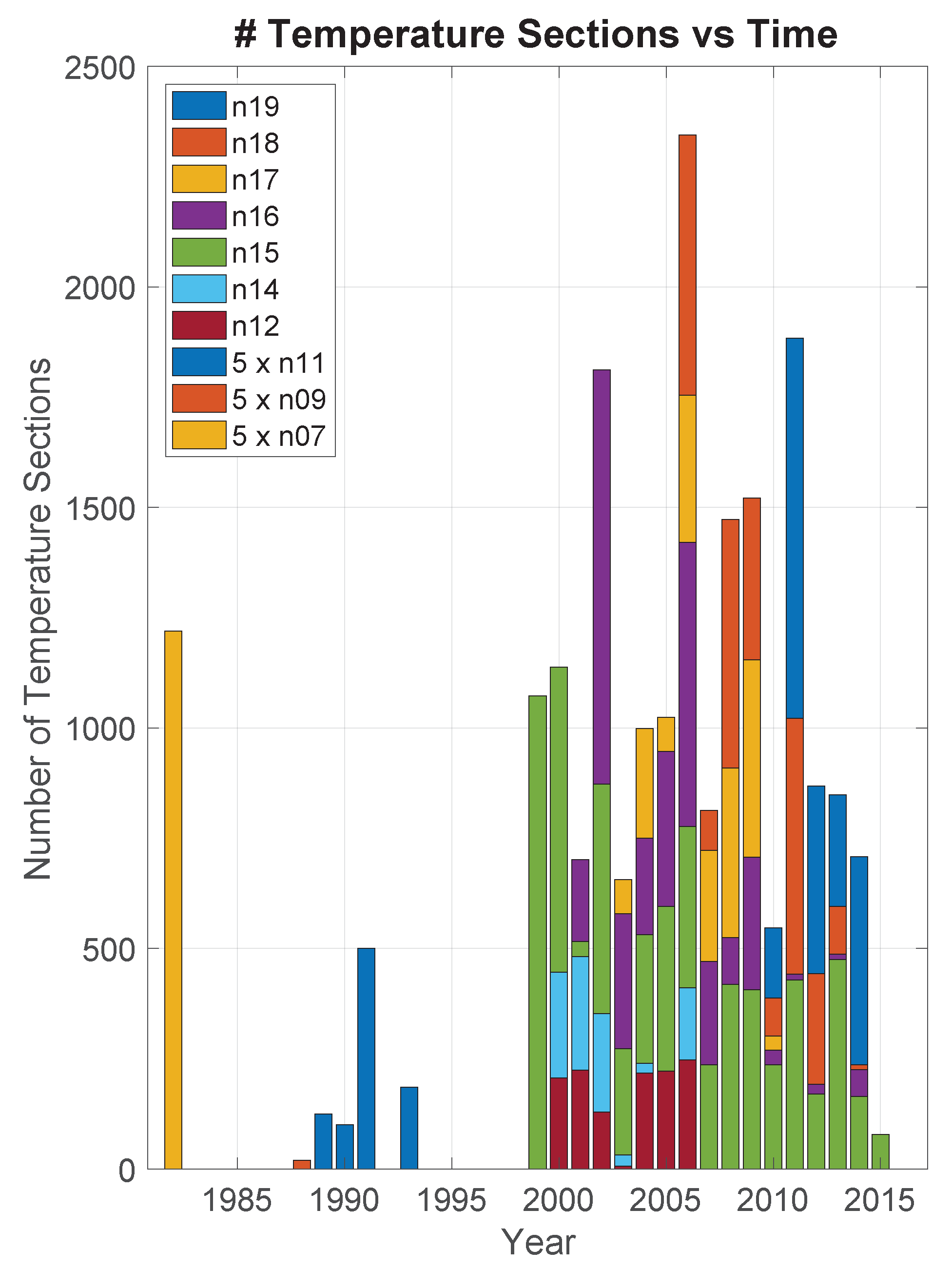
Table 1 shows the period covered by each satellite as well as the number of along-scan and along-track sections by day and night. Figure 3 shows this information graphically except by year with along-track and along-scan sections summed. The numbers prior to 1998 have been multiplied by five in Figure 3 since they are quite small.
Individual spectra are too noisy to obtain meaningful estimates of the p2p —the PSD shown in Figure 2 is a seven spectrum average. The next step therefore involves averaging of the spectra. Because the shape and/or total energy may differ substantially from one section to the next, noise estimates are most reliable if the spectra averaged are similar in both shape and energy. Wu2017 achieved this by grouping spectra obtained from temperature sections adjacent in a given pass. This was done in part with an algorithm and in part manually. Beginning with the first, along-scan section in an image, the algorithm examined the difference between it and subsequent along-scan sections. When the difference exceeded a given threshold, all sections prior to that section were grouped and the associated spectra averaged. The section that failed the difference test was then used as the first in the next sequence. This continued for all sections in a given satellite pass. The algorithm did not perform as well as desired so the groups were then manually modified—either groups were joined into larger groups or further divided. This process was repeated for along-track sections. Given that the time of the satellite pass determines whether it is a daytime or nighttime pass, the groups identified here were members of a particular day-night, scan-track class. The spectra from all sections in a group were averaged and the noise associated with that group determined. The resulting noise values were then averaged for each of the four day-night, scan-track classes to obtain a noise estimate for that class. These are the values presented in Wu2017.
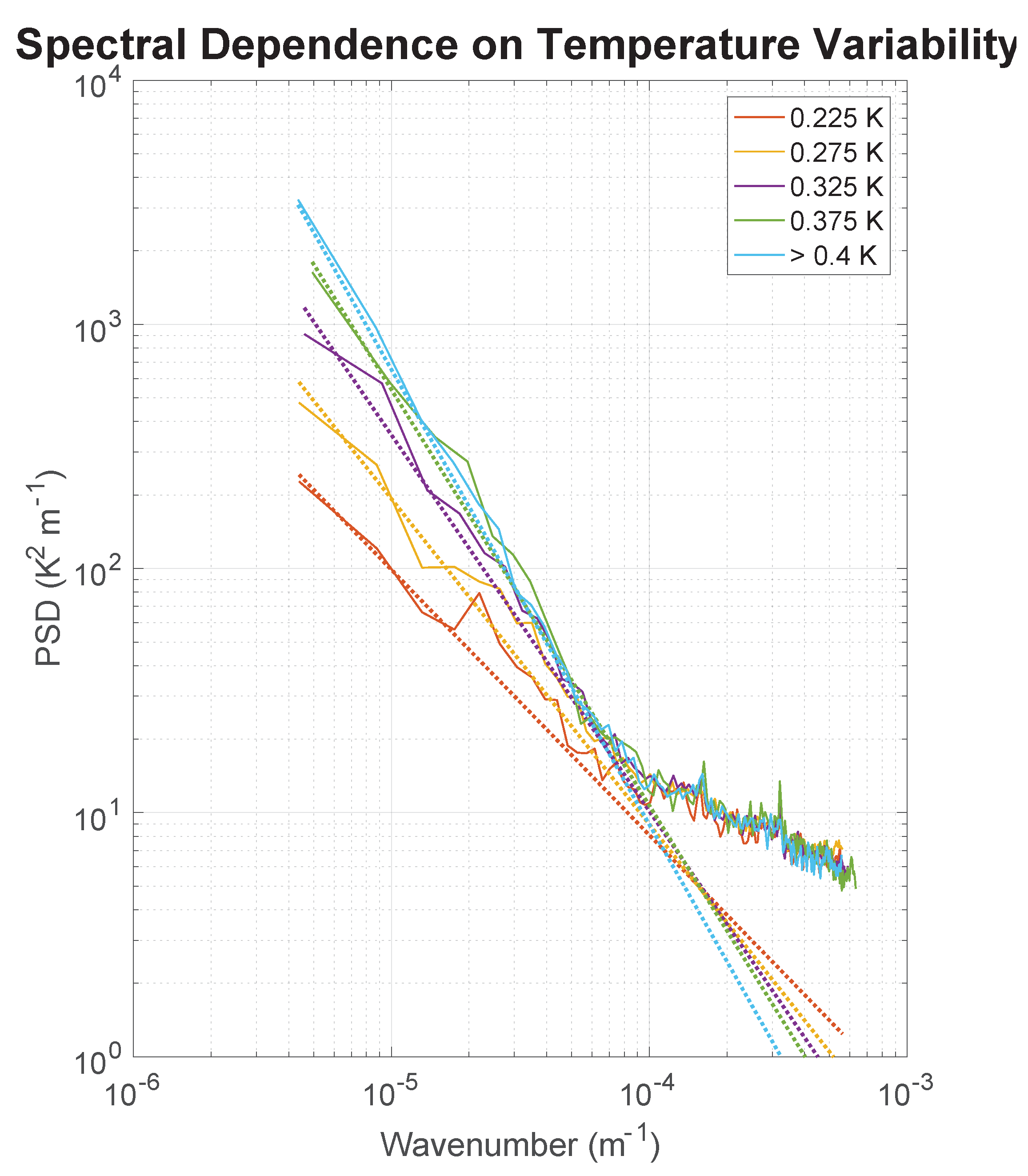
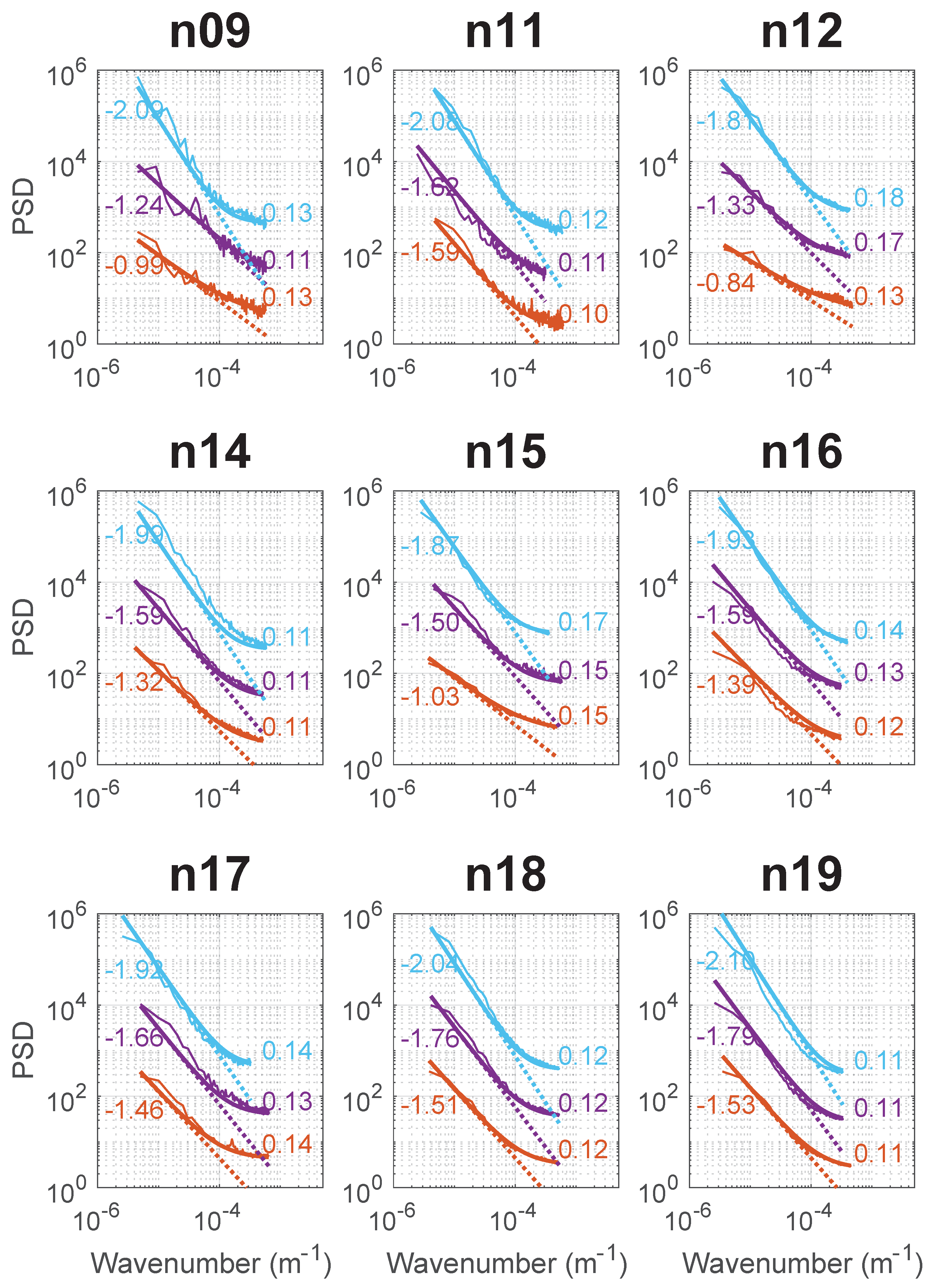
The approach outlined above does not scale well (it requires an inordinate amount of time) when applied to the data obtained from a number of satellites across a number of years and seasons and it introduced a level of subjectivity in the analysis, so we have adopted a different, purely objective approach. For each satellite, year, season, day-night, scan-track combination, we grouped sections by the standard deviation of the temperature values in the section, following detrending. Six groups were defined: 0 to 0.2 K, 0.2 to 0.25 K, 0.25 to 0.3 K, 0.3 to 0.35 K, 0.35 to 0.4 K and >0.4 K. As a result, we obtained noise estimates in a six-dimensional space—satellite (10), year (31), season (4), day-night (2), scan-track (2) and standard deviation (6), where the numbers in parentheses are the number of elements in the given dimension. The advantage of this approach is that not only is it objective (once the standard deviation thresholds have been identified), but it also allows the grouping of sections across satellite passes for a given element in this six-dimensional space, thus substantially smoothing the average spectra and improving the estimate of noise in the data. It also revealed an unexpected result—the underlying straight-line slopes (Equation (1)) of the best fit spectra increase with the standard deviation of temperature in the section. Figure 4 shows an example of this for the winter, 2011, daytime, along-scan, NOAA-15 mean spectra for temperature section standard deviations in excess of 0.2 K. (The smallest standard deviation group is not shown in Figure 4 because it is very noisy due to too few contributing sections. Consistent with the results for the larger standard deviation groups, the slope for the smallest standard deviation group is smaller than that of all other groups.) For wavenumbers greater than m (wavelengths smaller than 10 km), the spectra are virtually identical, dominated primarily by noise; i.e., there is little geophysical information in this portion of the spectrum. For smaller wavenumbers, the impact of noise decreases as the amount of energy in the spectrum increases. This is consistent with a similar analysis of the temperature spectra obtained from MV Oleander, which do not show a dependence on temperature section variance. Figure 5 shows similar information for NOAA-09 through NOAA-19. The dependence of slope on the variability of the underlying temperature sections is consistent from one AVHRR to another.
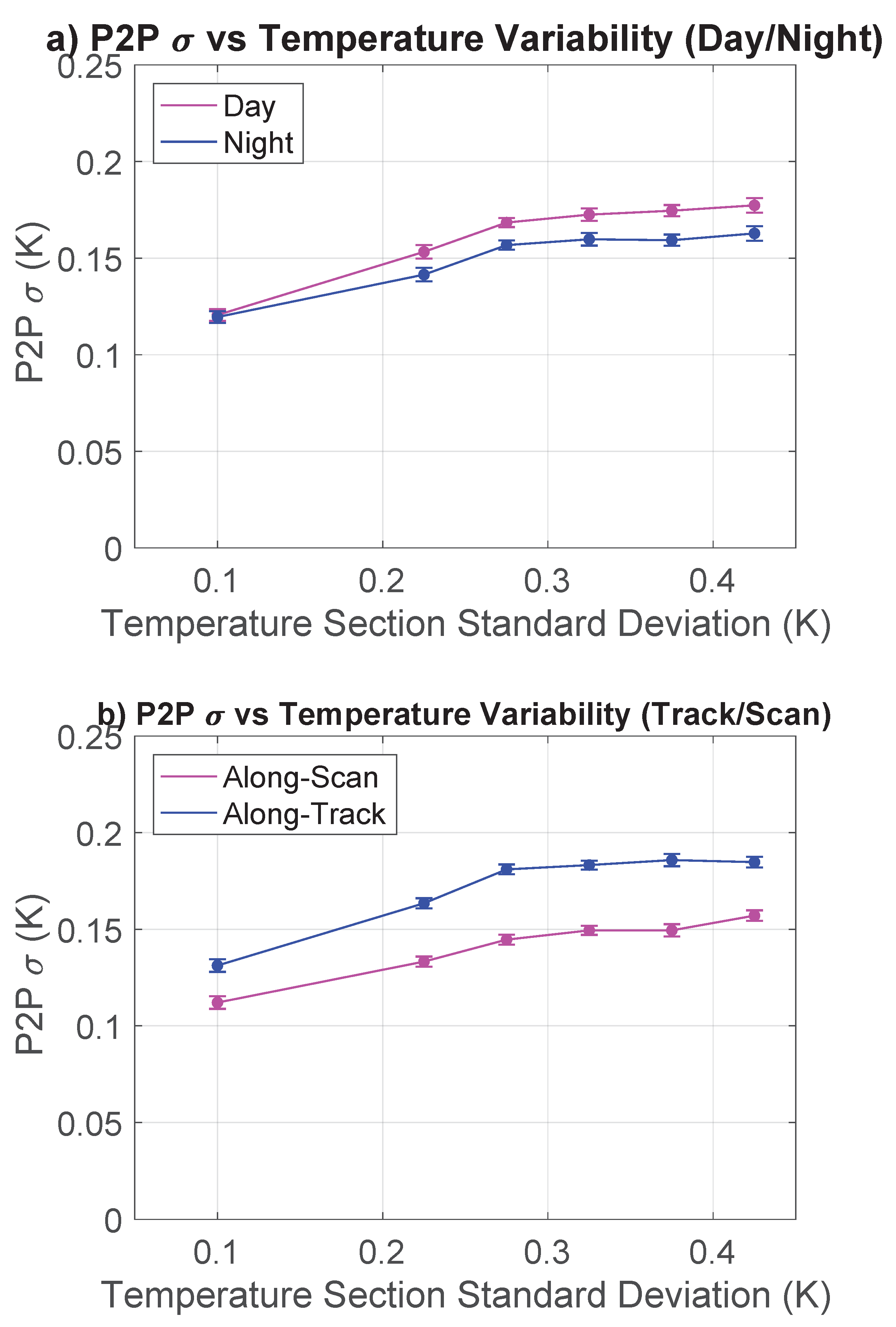
Of importance to the analysis undertaken herein, the estimated p2p is also a function of temperature variability (Figure 6). Specifically, the variability increases with temperature variability and this result is robust, occurring for daytime, nighttime, along-scan and along-track subsets. This is likely the case because the impact of noise is felt at smaller and smaller wavenumbers as the overall energy in the spectrum decreases while the noise in the satellite-derived SST fields remains the same—this noise does not depend on the geophysical variability in the scene. As the noise bleeds to smaller wavenumbers, it begins to affect the fit of the straight line to the lower wavenumber range, which is meant to represent the geophysical signal. The effect is to decrease the slope of the straight line spectrum, thus reducing the estimated variability. Basically, the p2p for the lower energy temperature sections is contributing to the determination of the slope. Consider the limiting case of the noise in the SST fields overwhelming the geophysical variability. Then, the resulting spectrum would be independent of wavenumber (assuming that the instrument noise is white) and the analysis would return instrument noise of zero attributing all of the energy in the spectrum to natural variability. Although the p2p “increases” with temperature variability, the rate of increase decreases with increasing energy remaining approximately constant for standard deviations of the temperature sections in excess of 0.25 K. In light of this, we restrict our analysis to temperature sections with a standard deviation in excess of 0.25 K.
4. Results
4.1. P2P by Satellite
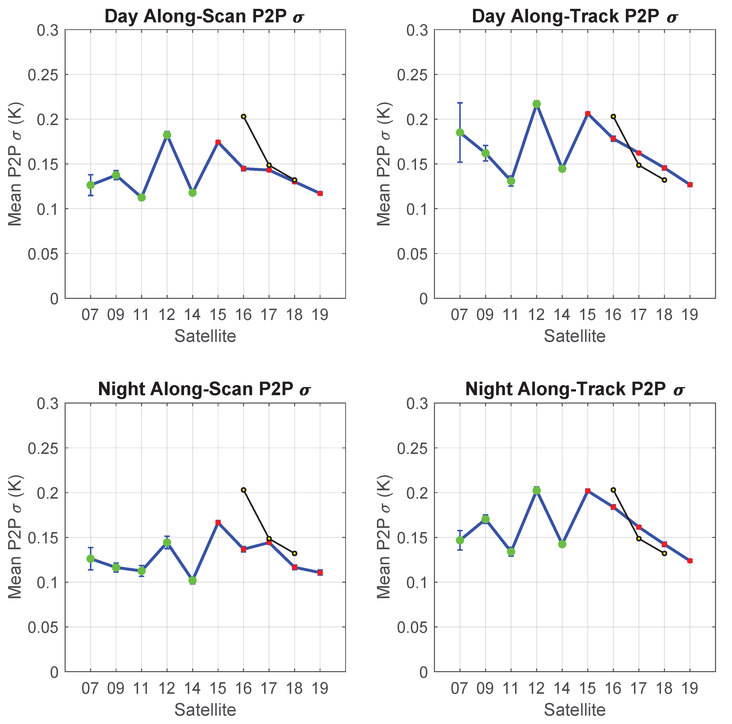
P2P for each of the satellites is shown in Figure 7 and tabulated in Table 2 for the four day-night, scan-track combinations. The values are averaged over all years, all seasons and all temperature standard deviation categories greater than 0.25 K. Also in the table are averages for all satellites. Although the grouping of temperature sections is, as discussed in Section 3, different from that used by Wu2017, the retrieved p2p values for NOAA-15 are well within the error bounds of the values obtained by Wu2017. The slight difference in values is likely due to the averaging intervals; the results of Wu2017 are averaged only for the summer of 2012 while those obtained in this study are averaged over all years and seasons for which we have NOAA-15 data. In addition, as found by Wu2017 for NOAA-15, there is little difference between the day and night values for either the along-scan or along-track sections, but there is a significant difference between the along-track and along-scan sections, with the latter being smaller than the former for all AVHRRs.
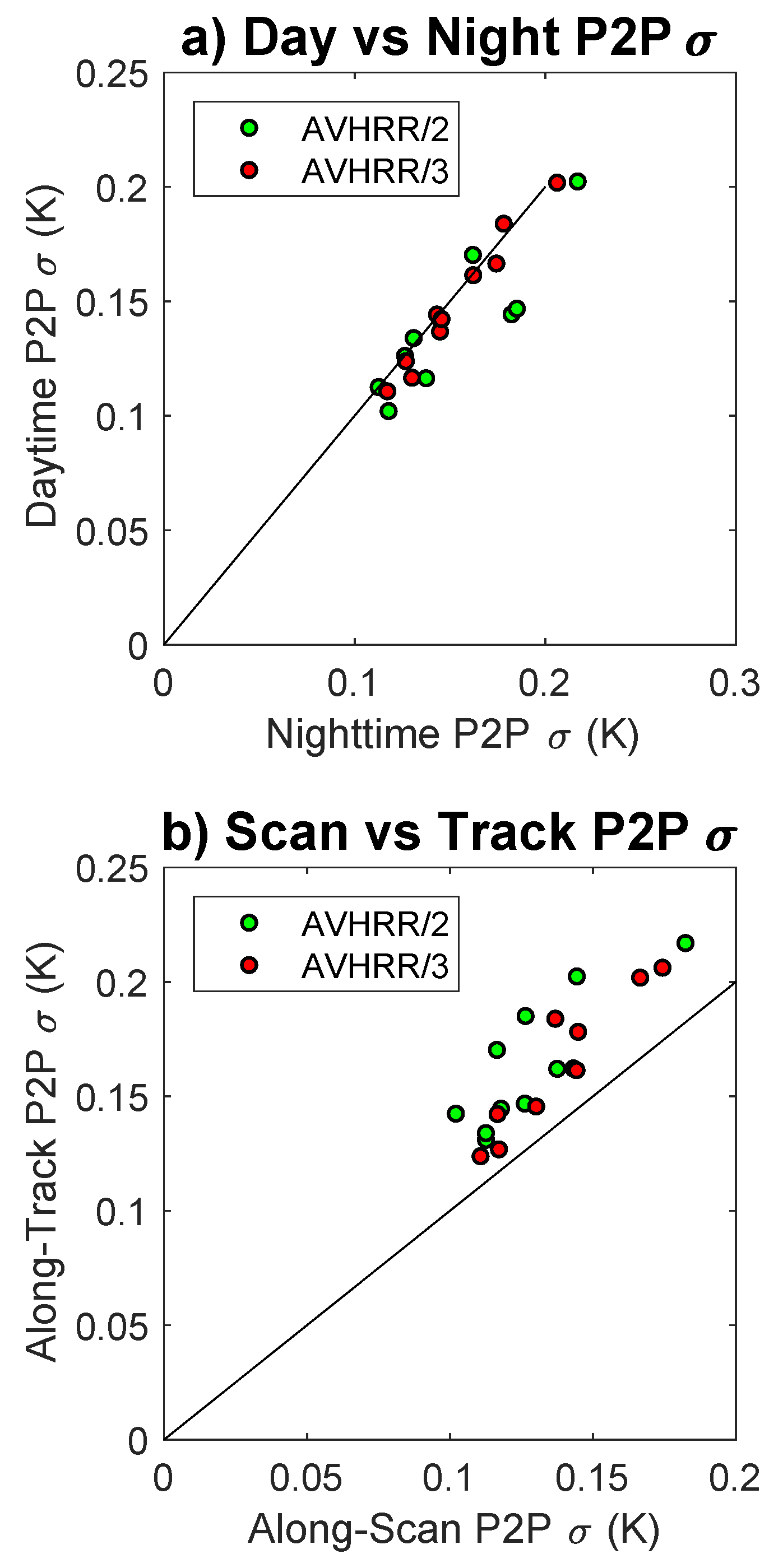
Building confidence that these estimates are satellite-specific and not simply random noise is the similarity of the shapes of the four curves shown in Figure 7. This is shown more clearly in Figure 8. Panel a is a plot of daytime versus nighttime p2p s. There are two points on the plot for each of the ten satellites, one for which all along-track estimates have been averaged and the other for the along-scan averages. Panel b shows a similar scatterplot for the along-scan versus along-track estimates, again ten points, this time averaging daytime estimates for one set of points and nighttime estimates for the other. In both cases, the points tend to line along lines close to parallel to the 1:1 line; i.e., a large value for a given satellite either day or scan combination corresponds to a similarly large value of the estimate for the same satellite either night or track combination. The offset of the points above the 1:1 line for the scan/track scatterplot (Figure 8b) is attributable to the variability in the calibration of the sensor from scan-line to scan-line. The higher correlation for both AVHRR/2 and AVHRR/3 points in the day/night scatterplot than for those in the scan/track scatterplot results from the satellite-to-satellite variability in calibration. Both of these effects are explained in detail in Section 5.3. An interesting aspect of the results for AVHRR/3, evident in Figure 7, is the clear decrease in p2p from NOAA-15 through NOAA-19, which is evident in all day/night, scan/track combinations. This will be shown (Section 5.3) to result primarily from the form of the retrieval algorithm used to obtain SST from the AVHRR radiances.
4.2. Seasonal Dependence of P2P by Satellite
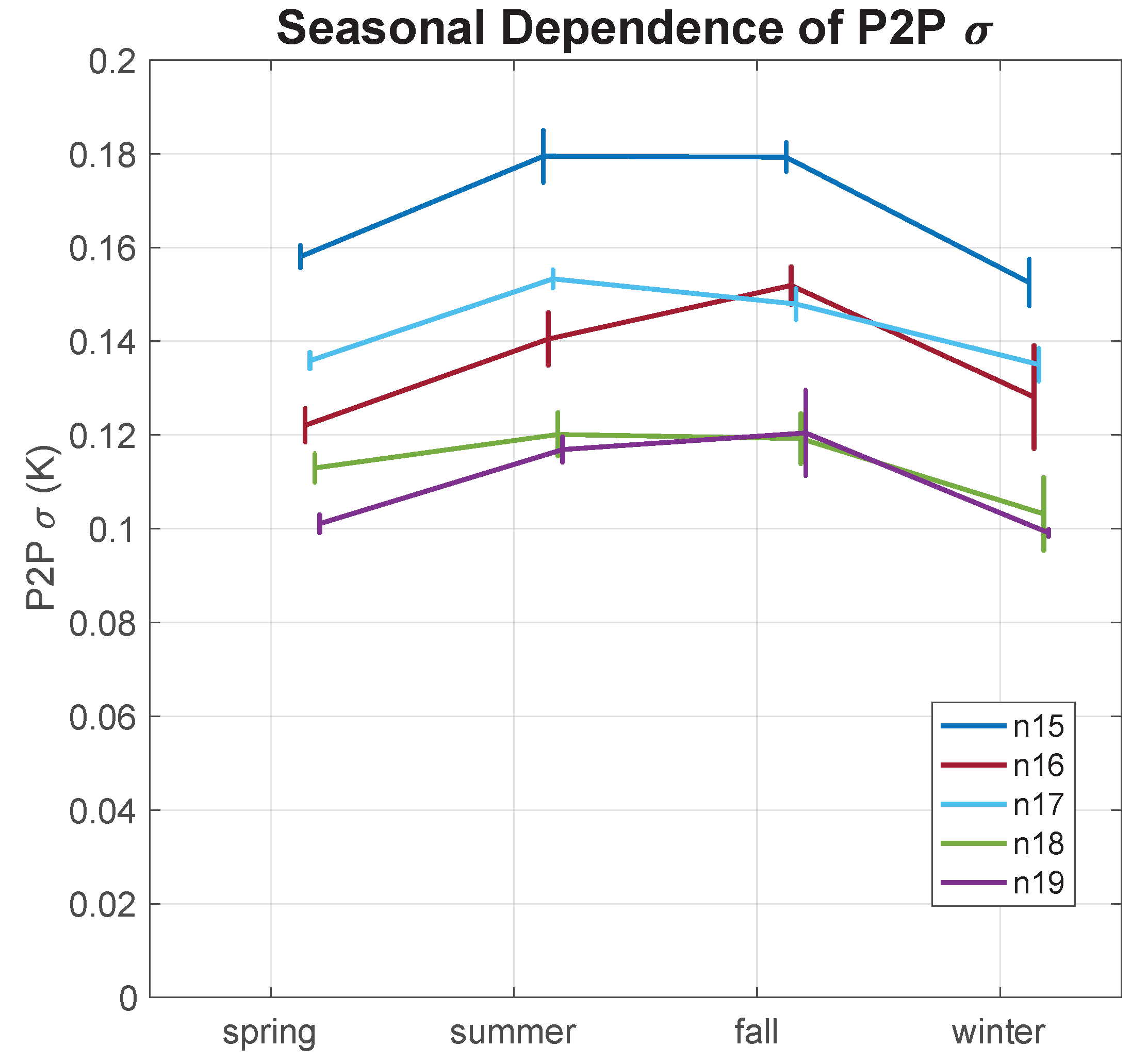
The seasonal dependence of p2p is shown in Figure 9. For clarity, only results for NOAA-15 through NOAA-19 are shown—the lines for the earlier satellites are more erratic but show the same general trends. Specifically, for all satellites, the p2p is higher in the summer and fall than in the winter and spring. This is shown to result from a decrease in the NEΔT of the individual sensors and, more consistently, a decrease from satellite-to-satellite of the water vapor correction term in the SST retrieval algorithm (Section 5.3).
4.3. Temporal Trend in P2P by Satellite
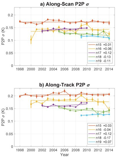
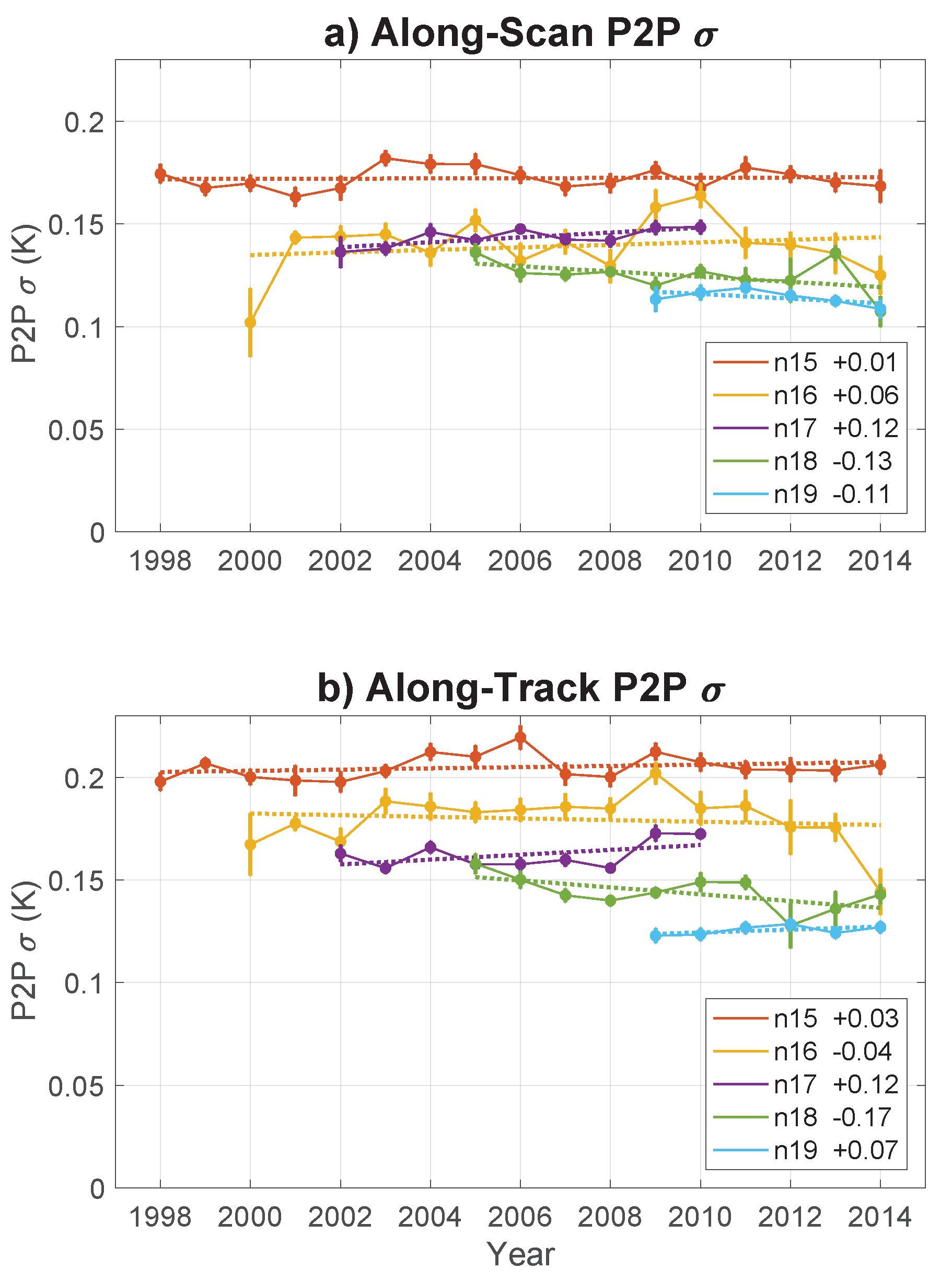
Temporal trends for the SST fields obtained from NOAA-15 through NOAA-19 are shown in Figure 10. Slopes of the best fit straight lines (values in the legend are in K/century) for NOAA-15, 16, 17 and 19 are small, with changes in the along-scan and along-track p2p less than 0.01 K over the life of the instruments. The trends in NOAA-18 are slightly larger, with decreases of 0.013 K and 0.017 K in the along-scan and along-track variability, respectively, over the life of the instrument. The reason for these decreases is unclear.
5. Discussion
The pixel-to-pixel variability of SST fields obtained from satellite-borne instruments results from the retrieval algorithm and varibiility in the calibrated radiances obtained by the instrument, which are used in the retrieval algorithm to estimate temperature. Many of the characteristics of the p2p s, which we introduce above, may be understood from the perspective of these two contributors so we address the relevant aspects associated with them in some detail in the following two subsections and then discuss these in the context of our results.
5.1. Pathfinder Retrieval Algorithm
The basic form of the Pathfinder retrieval algorithm [8] is:
where and are the Brightness Temperatures (BTs) for channels 4 and 5 discussed in the next section, SST is a first-guess SST for the pixel obtained from another source of data (the ‘Reynolds’ optimally interpolated 1/4, daily fields [9] for the Pathfinder datasets), is the satellite zenith angle and a, b, c and d are coefficients determined by linear regression. The regression is performed on a match-up database consisting of in situ measures and and BTs obtained within ±30 min and of latitude and longitude of the in situ measure. Coefficients were determined for two ranges, those values C and those C.
Assuming statistical independence of the BT uncertainties [10], they propagate through the retrieval algorithm as:
where indicates the variance of the quantity relative to the local mean (over several pixels; i.e., not incorporating the atmospheric variance) and . Because we made use only of temperature sections within 500 km of nadir, is small and the term is negligible leaving us with:
b is very close to 1 and, in the Sargasso Sea, the area from which the temperature sections were extracted, ranges from 1.5 to 4—for all of the radiometers considered, determined from for C and for C times the first guess SST, which ranges from C to C in the study area. This means that the variability in the term is the dominant contributor to the variability in retrieved SST, both because the coefficient of this term is larger than that of the term and because the sum of the variance of both channels multiplies this term. For , uncertanties associated with the term are between 2 and 5 times those of the alone term (more on this in Section 5.3).
5.2. Uncertainties in Brightness Temperature (BT)
As noted above, uncertainties in the BTs are at the base of the p2p s in the retrieved SST values. Uncertainties in the BTs are usually quoted as NEΔTs. However, the meaning of NEΔT varies from provider-to-provider. From the perspective of this paper, there are three basic components contributing to this variability: electronic noise in the instrument, calibration of the instrument and the digitization of the electronic signal observed by the detector [11]. In some cases [12], NEΔT represents the variability of the electronic noise in the instrument plus that associated with the calibration, while, in other cases [13], NEΔT includes the contribution of all three terms. Variability introduced by the digitization of the signal depends on the temperature range measured by the sensor, the temperature of the target (due to the nonlinearity of the Planck Function) and the number of counts into which the temperature range is divided. For AVHRR instruments, the temperature range is 180 K to 335 K digitized into 1024 counts; i.e., one digital count spans approximately 0.12 K ⓐ 300 K. The variability of a top hat distribution is times the width of the distribution, 0.12 K in this case, so this term is on the order of 0.035 K. This term is generally independent of the instrument. The other two contributions depend on the instrument and on how the calibration is performed.
The radiometric characteristics required for calibration were determined for each of the AVHRR instruments before launch. Pre-launch calibration was performed under ideal conditions, not conditions encountered in space, such as changes in spacecraft temperature and stray radiation entering the instrument, both occurring over relatively short time frames (minutes to tens of minutes), and long-term on-orbit degradation of the sensors themselves occurring over much longer time frames [14,15,16,17]. Recognizing this, these instruments were also equipped with an on-board calibration capability, which is the primary information used by most SST retrieval algorithms to relate the electronic signals from the detectors to radiance impinging on the detectors. In light of this, we do not dwell on the pre-launch calibration since it has only a marginal impact on the p2p s of Pathfinder SSTs, this through the nonlinearity correction mentioned briefly below. In addition, pre-launch calibration information is not readily accessible in the open literature for AVHRR instruments, although this information has been obtained for some of the radiometers and used to better understand their characteristics. Those interested in a more detailed description of pre-launch calibration are referred to the work of Brown et al. [14] and Mittaz et al. [18].
The primary concern with regard to in-flight calibration relates to the long-term stability of the instruments (to mention a few, [14,15,17,19]) and there continues to be work in this area to improve the calibration [18,20,21,22]. Although many of the issues related to the long-term stability of the instruments are of little consequence to the p2p , some are, so we briefly summarize the in-flight calibration available in the L1b fields used for the Pathfinder retrievals.
In-flight calibration is performed on a scan-by-scan basis. Because only channels 4 and 5, observed in the 10–12 m atmospheric window, are used for the Pathfinder retrievals discussed in this paper, the remainder of this section addresses in-flight calibration for these. For each scan of the radiometer, each detector acquires 10 views of deep space, 10 views of the Internal Calibration Target (ICT) and 2048 samples of the top-of-atmosphere looking down, the data of interest. In addition, four Platinum Resistance Thermistors (PRTs) determine the temperature of the ICT [23,24]. The radiance of the deep space view is very close to that of a 3 K blackbody, while that of the ICT is from a blackbody between 286 K and 300 K [17] for which the temperature is known. This provides two points, the average of the 10 deep space values and the average of the 10 ICT values, with known temperatures and corresponding electronic signals (digital counts) from which a linear relation between radiance (converted to BT via the Planck Function) and digital counts is estimated. There is a slight nonlinearity in the detectors, which, for each AVHRR, was determined in the pre-flight calibration and not thought to change significantly in-orbit. The linear relation is corrected to account for the nonlinearity and the resulting relationship is used to convert digital counts, for the portion of the scan when the detector is viewing Earth, to BTs. For each pixel, there are two BT values, one for channel 4 (10.3 to 11.2 m, in Section 5.1) of the radiometer and one for channel 5 (11.5 to 12.5 m, ). These BTs are used in Equation (2) to estimate SST in cloud-free regions.
5.3. Putting It All Together
In this section, we examine our p2p results in the context of the Pathfinder retrieval algorithm and the NEΔTs of the BTs used in the algorithm. We begin by estimating the p2p for the AVHRRs on NOAA-16, 17 and 18 based on NEΔT values available from NOAA’s Sensor Stability for SST (3S) system [13]. These three instruments, all AVHRR/3s, were chosen based on the availability of the regression coefficients for the retrieval algorithm (Equation (2)) and our decision to restrict this portion of the analysis to AVHRR/3s for which we have much more data than for the AVHRR/2 instruments, hence the results are much more stable. In Table 3, we tabulate the estimated means as well as the ranges for the 3S and NEΔTs. Also shown in the table are the mean values of the coefficient of the term. These were obtained by averaging the product of the C regression coefficient, c (Equation (2)), times the climatological SST at 33N, 68W, obtained from the World Ocean Atlas 2005 (WOA05) for the corresponding value of c [25]. (c is determined on a monthly basis and is correlated with SST through the regression, hence the need to take the product of the two before averaging.) Finally, the p2p s, based on the mean s, s and s introduced into Equation (3), were estimated with . These values, also included in Table 3, are plotted in Figure 7; the thin black line with data values indicated in yellow. Two observations are relevant with regard to these results. First, the estimated values are, on average, consistent with the along-track p2p s obtained spectrally from the SST fields, lending credence to the procedure. Because the NEΔTs used include the contribution of calibration and the calibration varies in time, one would expect the estimates to be closer to the along-track results than the along-scan results, which do not include a significant contribution from the variability in the calibration. Second, the decrease in p2p from NOAA-16 to NOAA-18 is determined both by a decrease in and a decrease in and . It is not clear why the coefficient is satellite-dependent. It may not be, it may simply be a coincidence. Regardless, the apparent satellite dependence is a bit disconcerting for those using Pathfinder SST fields to study trends in front probability or performing gradient analyses of SST fields obtained from AVHRR instruments on different satellites.
Also attributable to the term is the well defined seasonal trend, Figure 9, evident for all AVHRR/3s (we did not examine this for AVHRR/2s). Plots of the p2p seasonal s obtained from Equation (3) (not shown) are very similar in shape to those obtained from the satellite data (Figure 9), with, for all three satellites studied in detail, NOAA-16 through NOAA-18, summer and fall values always larger than winter and spring values. Because the relationship between the summer and fall values is not as well defined as the winter/spring vs. summer/fall differences, presumably because of the interannual variability of the SST annual cycle, we examine the ratio of the difference between the averaged winter and spring values and the averaged summer and fall values and the sum of these averages:
These ratios are presented in Table 3 both for the p2p s obtained spectrally from the satellite data and for those estimated with Equation (3). Although somewhat different in magnitude, the signs and the satellite-to-satellite differences are similar for the estimates obtained from the SST fields and the p2p s calculated from Equation (3).
Both the dependence of the satellite-to-satellite differences in the p2p and the consistency in their seasonal variability for each of the satellites clearly show the importance of the term in determining the p2p . Given that the term corrects for atmospheric attenuation of the upwelling radiation and that, in general, the atmosphere varies more slowly spatially than the ocean, averaging the term over an pixel region should reduce the contribution of this term to the p2p by approximately a factor of n without significantly impacting the overall accuracy of the retrievals. Barton [26] suggested precisely this; specifically averaging over a ‘ or ’ pixel array should reduce the p2p . Miller et al. [27], based on Barton’s observation, implemented this approach in the retrieval system developed by the Remote Sensing Group at the Plymouth Marine Laboratory, UK. They found that ‘a window size of 17.5 km square was appropriate for smoothing sensor noise while retaining the water vapour structure.’ Not long after, P. Le Borgne [28] of the Centre de Météorologie Spatiale (CMS), found a reduction of a little less than 50% in the standard deviation of SST values obtained from the Spinning Enhanced Visible and Infra-Red Imager (SEVIRI), a sensor carried on a geostationary satellite, when the term [29] was averaged over pixel squares compared with SST retrievals from the same algorithm but without averaging the term. Furthermore, this reduction increased as the size of the region over which the average is performed increased but not as fast as the multiplicative inverse, which one would expect if it were due simply to the number of elements contributing to the average. This is because the geophysical variability in the SST field contributes to the variance and this contribution increases as the size of the region increases; specifically, there was little benefit when averaging over more than pixel squares for which the reduction in SST variance was a bit less than 50%. It is important to keep in mind that the measure he used was based on the SST variance, which, as noted above includes the natural variability in the SST field. The natural variability in the SST field is not likely to contribute significantly to the term, although the natural variability in the atmosphere will, but on a scale that is large compared with pixel-to-pixel scale. Furthermore, averaging the term does not affect the contribution of the term, which is not averaged, to the variability. Based on Le Borgne’s observations, averaging was included in the operational processing of the SEVIRI data stream to SST, as well as of the EUMETSAT AVHRR stream to SST, and continues to present [30,31]. Note that SEVIRI pixels are order km, hence a pixel region is order km. This seems a bit large but an analysis similar to that undertaken by Le Borgne or Miller et al. [27] should be undertaken for the Pathfinder retrieval algorithm to determine the appropriate scale over which to average the term.
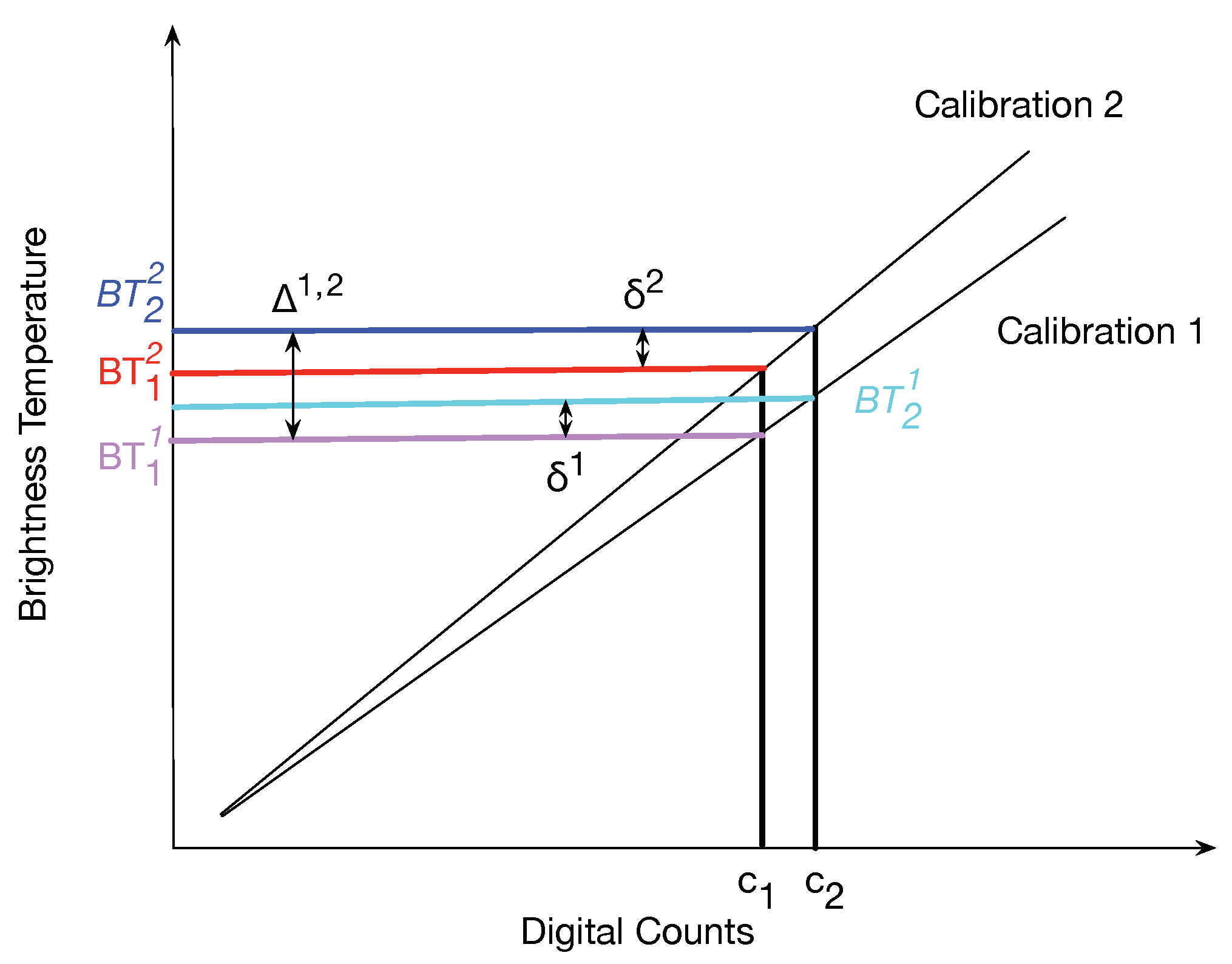
Next, we examine the along-scan, along-track differences (Figure 7, Figure 8b and Figure 10), which are directly attributable to the way the data have been calibrated. Specifically, calibration is performed on a line-by-line basis—it is constant for all pixels on a given scan line. This means that the calibration only affects the along-scan p2p through the scale factor used in converting from digital counts to BT, which, assuming that the calibration is close to the correct value, will be very small; i.e., the impact of the error in the calibration on the p2p along a scan line is small. This is shown schematically in Figure 11. The difference in the BTs of two adjacent pixels on a scan line with calibration 1 is (the superscript indicating the number associated with the calibration, not an exponent). For the same two pixels, the difference in BT would be for calibration 2. Even though the calibration lines differ substantially, the two s are very close. However, for two adjacent pixels in the along-track direction, the calibration for the two pixels may be different. In the example of Figure 11, the resulting differences in BTs for a similar difference in digital counts are , substantially larger than either of the s. Statistically, the variability in the calibration increases the p2p in the along-track direction, hence the differences between along-scan and along-track p2p s in Figure 6b, Figure 7, Figure 8b and Figure 10 as well as the differences documented in Table 2. If we assume that the variability due to instrument noise is not correlated with that due to calibration and that neither of these are correlated with the digitization noise, we can estimate the contribution to the p2p from the along-scan/along-track differences. The along-track variability is given by:
where is the p2p , is the contribution due to instrument electronics, is the contribution due to calibration and is the contribution due to digitization. In that the calibration is constant by scan line, the along-scan variability is given by:
Combining the two equations, we get:
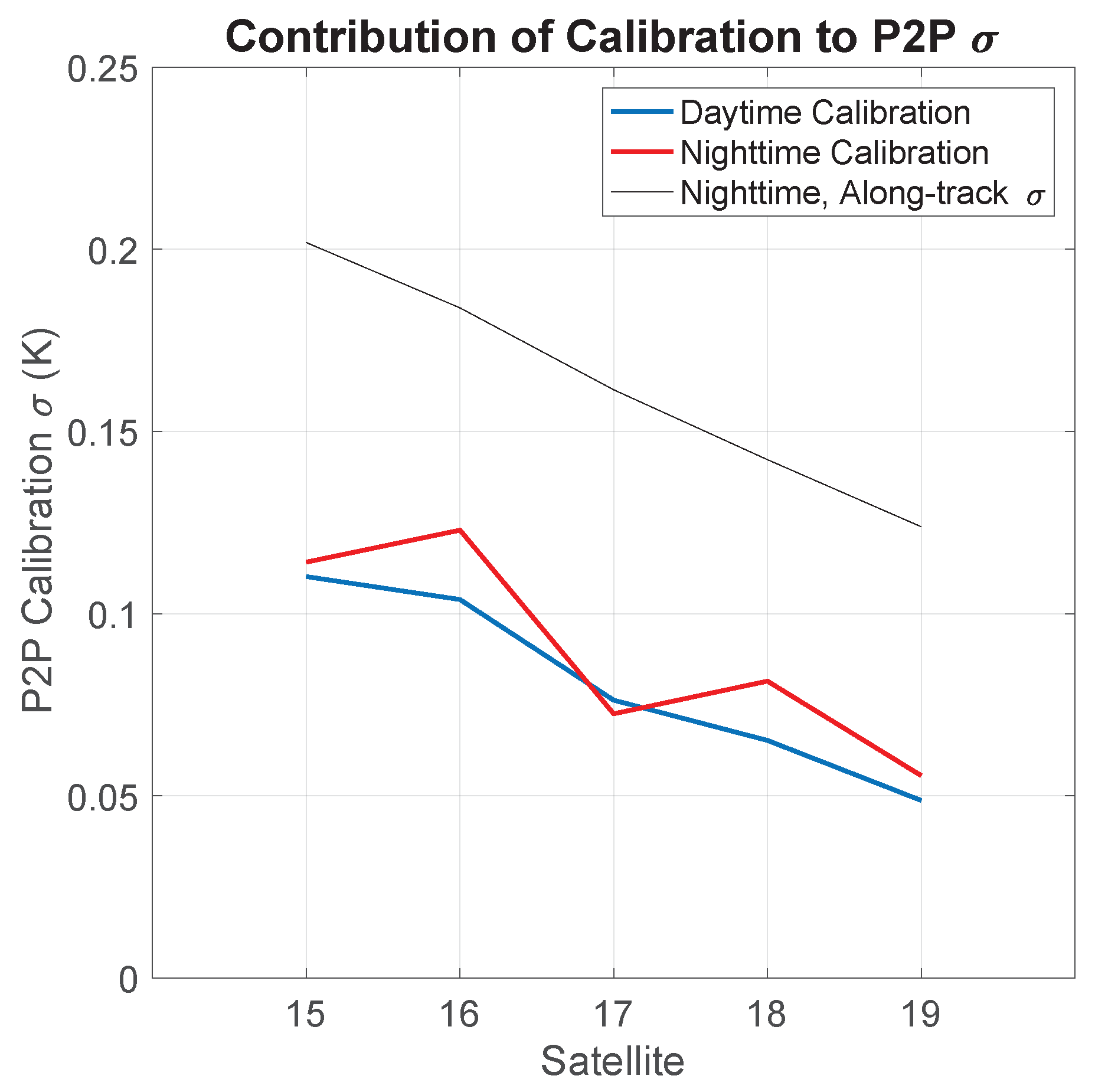
both of which we know. The contribution of the calibration to the variability determined from Equation (5) is shown in Figure 12 for both daytime and nighttime for the satellites carrying AVHRR/3 instruments. Note that the contribution to the variability attributed to the calibration here is only that for scan-to-scan fluctuations in the calibration. There are a number of factors, which contribute to variability in the calibration on scales larger than a few pixels, but these do not affect the p2p .
6. Conclusions
Using the spectral approach introduced by Wu2017, the p2p has been estimated for NOAA-07, 09, 11, 12 and 14–19. These estimates have been stratified by year, season, day/night and along-scan/along-track. Overall, the p2p values range from 0.10 K for NOAA-14 along-scan, nighttime fields to 0.21 K for NOAA-12 along-track, daytime fields. For each satellite, the along-scan value is between 10 and 20% smaller than the along-track value (except for NOAA-16 nighttime for which it is approximately 30% smaller). These differences were used to estimate the contribution of variability in the calibration to the p2p in the along-track direction. These are a lower bound on the contribution of calibration errors to the accuracy of the sensors in that the accuracy incorporates longer period errors than those contributing to the p2p s. It was also shown for each satellite that the summer and fall p2p s are between 10 and 15% smaller than the winter and spring values. The seasonal differences result from the term in the algorithm used for Pathfinder SST retrievals. This term is shown to be a major contributor to the p2p , suggesting that its impact could be reduced substantially by averaging it as part of the retrieval process without a deleterious effect on the overall p2p of the resulting products.
With the exception of NOAA-17 and NOAA-18, the trends, for AVHRR/3 instruments, in p2p result in changes over the life of the instrument that are small compared with the inter-satellite differences. This is true for both along-scan and along-track values. NOAA-17 shows a linear increase in time of approximately 0.001 K/year over the 10 years available in the URI archive and NOAA-18 shows a similar decrease. Over the lifetime of the sensors, this corresponds to a change in p2p similar to that seen between instruments. With regard to inter-instrument values, the p2p decreases close to linearly from NOAA-15 through NOAA-19. Analysis based on the NEΔTs available from NOAA’s Sensor Stability for SST system suggests that this decrease results primarily from a decrease in the NEΔTs of the BTs obtained from these instruments.
Author Contributions
Conceptualization, P.C.; Data curation, K.K.; Formal analysis, F.W. and P.C.; Investigation, F.W.; Methodology, F.W., P.C. and L.G.; Software, F.W. and P.C.; Supervision, P.C. and L.G.; Validation, K.K.; Visualization, F.W.; Writing—original draft, F.W.; Writing—review and editing, P.C., L.G. and K.K.
Funding
This research was supported by the National Programme on Global Change and Air-Sea Interaction (GASI-02-PACIND-YGST-03), the Global Change Research Program of China (2015CB953901), the National Natural Science Foundation of China-Shandong Joint Fund for Marine Science Research Centers (U1606405), the National Natural Science Foundation of China (41376105, 41574014, 41774014), the National Oceanographic and Atmospheric Administration (NA11NOS0120167), the National Aeronautics and Space Administration (NNX16AI24G and contract number: 80NSSC18K0837), the Frontier Science and Technology Innovation Project of the Science and Technology Commission of the Central Military Commission (085015), the Innovation Workstation Project of the Frontier Science and Technology Commission of the Central Military Commission, and the Outstanding Youth Fundation of the China Academy of Space Technology. Salary support for P.C. was provided by the state of Rhode Island and Providence Plantations.
Acknowledgments
The authors gratefully acknowledge contributions from Alexander Trishchenko and Alexander Ignatov for help in understanding issues related to AVHRR calibration and the authors offer special thanks to Pierre Le Borgne, Peter Minnett and Jonathon Mittaz for the many e-mails addressing a variety of issues related to the manuscript! We thank the Estimating the Circulation and Climate of the Ocean (ECCO) for making available output from the LLC4320 simulation and the NASA Advanced Supercomputing (NAS) Division of the Ames Research Center for providing high-end computing resources.
Conflicts of Interest
The authors declare no conflict of interest.
Abbreviations
The following abbreviations are used in this manuscript:
| AVHRR | Advanced Very High Resolution Radiometer |
| BT | Brightness Temperature |
| CLASS | Comprehensive Large Array-data Stewardship System |
| CMS | Centre de Météorologie Spatiale |
| FFT | Fast Fourier Transform |
| GHRSST | Group for High Resolution Sea Surface Temperature |
| HRPT | High Resolution Picture Transmission |
| ICT | Internal Calibration Target |
| LLC | Latitude/Longitude/polar-Cap |
| LLC-4320 | Latitude/Longitude/polar-Cap (LLC)-4320 |
| NASA | National Aeronautics and Space Administration |
| NEΔT | Noise Equivalent Temperature |
| NOAA | National Oceanic and Atmospheric Administration |
| NPP | National Polar-orbiting Partnership |
| p2p | pixel-to-pixel |
| PRT | Platinum Resistance Thermistor |
| PSD | power spectral density |
| SEVIRI | Spinning Enhanced Visible and Infra-Red Imager |
| 3S | Sensor Stability for SST |
| SST | sea surface temperature |
| URI | University of Rhode Island |
| VIIRS | Visible-Infrared Imager-Radiometer Suite |
| WOA05 | World Ocean Atlas 2005 |
References and Notes
- Wu, F.; Cornillon, P.C.; Boussidi, B.; Guan, L. Determining the Pixel-to-Pixel Uncertainty in Satellite-Derived SST Fields. Remote Sens. 2017, 9, 877. [Google Scholar] [CrossRef]
- ‘Level-2’ refers to the processing level of the data, a nomenclature used extensively for satellite-derived datasets, although the precise meaning of the level of processing varies by organization. The definition used here, http://science.nasa.gov/earth-science/earth-science-data/data-processing-levels-for-eosdis-data-products/, is that promulgated by the GHRSST.
- Cornillon, P.; Castro, S.; Gentemann, C.; Jessup, A.; Kaplan, A.; Lindstrom, E.; Maturi, E. SST Error Budget—White Paper; Technical Report; University of Rhode Island: Kingston, RI, USA, 2010; Available online: https://works.bepress.com/peter-cornillon/1/ (accessed on 24 February 2019).
- Obenour, K.M. Temporal Trends in Global Sea Surface Temperature Trends. Master’s Thesis, University of Rhode Island, Kingston, RI, USA, 2013. [Google Scholar]
- Kahru, M.; Di Lorenzo, E. Spatial and temporal statistics of sea surface temperature and chlorophyll fronts in the California Current. J. Plankton Res. 2012, 34, 749–760. [Google Scholar] [CrossRef] [Green Version]
- Rocha, C.B.; Chereskin, T.K.; Gille, S.T.; Menemenlis, D. Mesoscale to Submesoscale Wavenumber Spectra in Drake Passage. J. Phys. Oceanogr. 2016, 46, 601–620. [Google Scholar] [CrossRef]
- Vazquez-Cuervo, J.; Torres, H.S.; Menemenlis, D.; Chin, T.M.; Armstrong, E.M. Relationship between SST Gradients and Upwelling off Peru and Chile: Model/Satellite Data Analysis. Int. J. Remote Sens. 2017, 38, 6599–6622. [Google Scholar] [CrossRef]
- Kilpatrick, K.A.; Podestá, G.P.; Evans, R. Overview of the NOAA/NASA advanced very high resolution radiometer Pathfinder algorithm for sea surface temperature and associated matchup database. J. Geophys. Res. 2001, 106, 9179–9198. [Google Scholar] [CrossRef]
- Reynolds, R.W.; Smith, T.M.; Liu, C.; Chelton, D.B.; Casey, K.S.; Schlax, M.G. Daily High-Resolution-Blended Analyses for Sea Surface Temperature. J. Clim. 2007, 20, 5473–5496. [Google Scholar] [CrossRef]
- The noise in channels 4 and 5 may be correlated. Furthermore, there are a number of other characteristics affecting the calibration, which are not included in the brief overview of calibration presented in Section 5.2. Jonathan Mittaz, personal communication, 24 January 2019.
- Issues related to in-flight calibration are more complicated than suggested here. Jonathan Mittaz, personal communication, 24 January 2019. However, with the exception of the possible correlation between channels and of the non-Gaussian nature of the noise, the extra complexity does not play a significant role in the analysis presented here.
- Rama Varma Raja, M.K.; Battles, D.; Wu, X.; Bauch, H.; Yu, F.; Lambeck, R.W.; Sun, N.; Perez Albinana, A.; Montagner, F. In-Orbit Health and Performance of Operational AVHRR Instruments; SPIE Optical Engineering + Applications, Strojnik, M., Paez, G., Eds.; SPIE: Bellingham, WA, USA, 2010; p. 780814. [Google Scholar]
- He, K.; Ignatov, A.; Kihai, Y.; Cao, C.; Stroup, J. Sensor Stability for SST (3S): Toward Improved Long-Term Characterization of AVHRR Thermal Bands. Remote Sens. 2016, 8, 346. [Google Scholar] [CrossRef]
- Brown, O.B.; Brown, J.W.; Evans, R.H. Calibration of advanced very high resolution radiometer infrared observations. J. Geophys. Res. Oceans 1985, 90, 11667–11677. [Google Scholar] [CrossRef]
- Steyn-Ross, D.A.; Steyn-Ross, M.L.; Clift, S. Radiance calibrations for advanced very high resolution radiometer infrared channels. J. Geophys. Res. 1992, 97, 5551–5568. [Google Scholar] [CrossRef]
- Brown, J.W.; Brown, O.B.; Evans, R.H. Calibration of advanced very high resolution radiometer infrared channels: A new approach to nonlinear correction. J. Geophys. Res. Oceans 1993, 98, 18157–18269. [Google Scholar] [CrossRef]
- Trishchenko, A.P.; Fedosejevs, G.; Li, Z.; Cihlar, J. Trends and uncertainties in thermal calibration of AVHRR radiometers onboard NOAA-9 to NOAA-16. J. Geophys. Res. 2002, 107, 4778. [Google Scholar] [CrossRef]
- Mittaz, J.P.D.; Harris, A.R.; Sullivan, J.T. A Physical Method for the Calibration of the AVHRR/3 Thermal IR Channels 1: The Prelaunch Calibration Data. J. Atmospheric Ocean. Technol. 2009, 26, 996–1019. [Google Scholar] [CrossRef]
- Minnett, P.J.; Smith, D.L. Chapter 2.4—Postlaunch Calibration and Stability: Thermal Infrared Satellite Radiometers; Elsevier: Amsterdam, The Netherlands, 2014; Volume 47. [Google Scholar]
- Trishchenko, A.P.; Li, Z. A method for the correction of AVHRR onboard IR calibration in the event of short-term radiative contamination. Int. J. Remote Sens. 2001, 22, 3619–3624. [Google Scholar] [CrossRef] [Green Version]
- Mittaz, J.; Harris, A. A Physical Method for the Calibration of the AVHRR/3 Thermal IR Channels. Part II: An In-Orbit Comparison of the AVHRR Longwave Thermal IR Channels on board MetOp-Awith IASI. J. Atmos. Ocean. Technol. 2011, 28, 1072–1087. [Google Scholar] [CrossRef]
- Chang, T.; Wu, X.; Weng, F. Modeling thermal emissive bands radiometric calibration impact with application to AVHRR. J. Geophys. Res. Atmos. 2017, 122, 2831–2843. [Google Scholar] [CrossRef]
- Lauritson, L.; Nelson, G.J.; Porto, F.W. Data Extraction and Calibration of TIROS-N/NOAA Radiometers; Technical Report NESS 107; National Oceanographic and Atmospheric Administration: Silver Spring, ML, USA, 1979; Rev. 1 (1988) by W.G. Planet. [Google Scholar]
- PRT values are provided on a five scan cycle, with PRT1 on scan 1, PRT2 on scan 2, PRT3 on scan 3, PRT4 on scan 4 and no PRT value on scan 5. The sequence then repeats.
- The T4 − T5 ≥ 0.7 °C regime is more representative of the water vapor environment in the study area than the T4 − T5 < 0.7 °C regime hence its use. c tends to be larger for the T4 − T5 < 0.7 °C leading to slightly larger estimates of the p2p σ uncertainties, but the general trends are similar.
- Barton, I.J. Digitization effects in AVHRR and MCSST data. Remote Sens. Environ. 1988, 29, 87–89. [Google Scholar] [CrossRef]
- Miller, P.I.; Groom, S.; Mcmanus, A.; Selley, J.; Mironnet, N. Panorama: A Semi-Automated Avhrr and Czcs System for Observation of Coastal and Ocean Processes. In Proceedings of the Remote Sensing Society, San Diego, CA, USA, 30 July–1 August 1997; pp. 539–544. [Google Scholar]
- Detailed in an internal CMS report “Radiometric noise and atmospheric correction smoothing in the case of Meteosat08/SEVIRI”. Pierre Le Borgne, personal communication, 3 February 2019.
- T4 and T5 refer to the brightness temperatures of spectral channels 4 and 5 on AVHRRs. The corresponding channels on SEVIRI are labeled differently but, for consistency, we continue to refer to this as the T4 − T5 term.
- SEVIRI is an infrared radiometer in a geosynchronous orbit with similar spectral channels to the AVHRR. The basic form of the SEVIRI retrieval algorithm is similar to that of the Pathfinder retrieval algorithm.
- Saux Picart, S. Algorithm Theoretical Basis Document for MSG/SEVIRI Sea Surface Temperature Data Record; Technical Report OSI-250; EUMETSAT: Darmstadt, Germany, 2018. [Google Scholar]
Figure 1.
(a) sample SST (in C) field from LLC-4320. (c–g) SST field of subplot a with 0.07 K, 0.15 K and 0.4 K Gaussian noise added. (b,d,f,h) gradient magnitude (in K/km) of (a,c,e,g), respectively.
Figure 1.
(a) sample SST (in C) field from LLC-4320. (c–g) SST field of subplot a with 0.07 K, 0.15 K and 0.4 K Gaussian noise added. (b,d,f,h) gradient magnitude (in K/km) of (a,c,e,g), respectively.

Figure 2.
Ensemble averaged power spectral density over the seven NOAA-15, along-track, nighttime, summer 2012, spectra for temperature sections with detrended standard deviations between 0.35 and 0.4 K (light blue). Heavy dotted black line is the underlying linear (in log–log space) portion of the fit, and the heavy red line is the linear fit plus noise.

Figure 3.
Number of temperature sections contributing to the derived statistics by year and by satellite. The numbers for the NOAA-07, NOAA-09 and NOAA-11, the numbers for years prior to 1998, have been multiplied by 5 to make them more visible. In addition, the colors used for data associated with these three satellites are similar to colors used for the data of three of the satellites flying after 1998, but there is no overlap in time for the duplicated colors, hence the usage should be clear.

Figure 4.
Average spectra by temperature section standard deviation groups for winter, 2011, daytime, along-scan NOAA-15 (solid lines). Dotted lines: best fit linear spectra following Equation (1).
Figure 4.
Average spectra by temperature section standard deviation groups for winter, 2011, daytime, along-scan NOAA-15 (solid lines). Dotted lines: best fit linear spectra following Equation (1).

Figure 5.
Spectral slope dependence on temperature section variability for all analyzed AVHRRs except that on NOAA-07 for which there were insufficient temperature sections for reliable estimates of the slope. Solid lines: best fit spectra to the mean spectra for standard deviation groups 0.2 to 0.25 K, 0.3 to 0.35 K, and >0.4 K following Equation (1). The mean spectra were obtained by averaging the spectra for spring, daytime and along-scan temperature sections. Dotted lines: the straight line only portion of the fit using Equation (1). For clarity, for each satellite, the curves for the 0.3 to 0.35 K standard deviation group were shifted up by a factor of 10 and those for the >0.4 K group by a factor of 100. Numbers to the left of each curve are the respective slopes. Numbers to the right are estimated p2p .

Figure 6.
Dependence of retrieved noise on the standard deviation of temperature in the sections for the given group. The data were averaged for the summer over all satellites and all years. Daytime/Nighttime plots also averaged along-scan and along-track estimates and along-scan/along-track plots averaged day and night estimates. Error bars are the standard deviation of the mean for the group. P2P levels are averaged over all satellites and over day and night for the upper plot and over along-scan and along-track for the lower plot.

Figure 7.
P2P versus satellite. Green circles: for AVHRR/2. Red circles: for AVHRR/3. Error bars are the standard error of the mean. Black line with yellow data values (repeated in all subplots) are estimated p2p based on NEΔT values (Section 5.1 and Section 5.3).
Figure 7.
P2P versus satellite. Green circles: for AVHRR/2. Red circles: for AVHRR/3. Error bars are the standard error of the mean. Black line with yellow data values (repeated in all subplots) are estimated p2p based on NEΔT values (Section 5.1 and Section 5.3).

Figure 8.
P2P versus satellite. Green circles are for satellites with AVHRR/2 instruments—NOAA-07, 09, 11, 12 and 14. Red circles are for satellites with AVHRR/3 instruments—NOAA-15, 16, 17, 18 and 19.
Figure 8.
P2P versus satellite. Green circles are for satellites with AVHRR/2 instruments—NOAA-07, 09, 11, 12 and 14. Red circles are for satellites with AVHRR/3 instruments—NOAA-15, 16, 17, 18 and 19.

Figure 9.
P2P by season for NOAA-15 through NOAA-19. Each data point is an average for the given satellite and the given season over all sections with standard deviations greater than 0.25 K. Error bars are the standard error of the mean.
Figure 9.
P2P by season for NOAA-15 through NOAA-19. Each data point is an average for the given satellite and the given season over all sections with standard deviations greater than 0.25 K. Error bars are the standard error of the mean.

Figure 10.
Temporal trends in p2p for NOAA-15 through 19. Upper panel: along-scan estimates. Lower panel: along-track estimates. Error bars are the standard error of the mean. Slopes in Kelvin per 100 years of the best-fit straight line to the multi-year data are provided to the right of the satellite name in the legend.

Figure 11.
Calibration schematic. BT subscripts correspond to the digital count, ‘1’ for and ’2’ for and the superscripts are associated with the calibration.
Figure 11.
Calibration schematic. BT subscripts correspond to the digital count, ‘1’ for and ’2’ for and the superscripts are associated with the calibration.

Figure 12.
Contribution of the calibration to the daytime (red) and nighttime (blue) p2p along-track variability. The nighttime p2p along-track variability (black) has been included for reference.
Figure 12.
Contribution of the calibration to the daytime (red) and nighttime (blue) p2p along-track variability. The nighttime p2p along-track variability (black) has been included for reference.


Table 1.
Coverage by Satellite.
| Satellite | Period Covered | Number of Sections | ||||
|---|---|---|---|---|---|---|
| Start | End | Day | Night | |||
| Along-Scan | Along-Track | Along-Scan | Along-Track | |||
| NOAA-07 | 01/04/82 | 07/09/82 | 233 | 89 | 25 | 68 |
| NOAA-09 | 05/20/85 | 10/25/88 | 716 | 280 | 273 | 741 |
| NOAA-11 | 02/22/89 | 08/14/94 | 1085 | 704 | 136 | 229 |
| NOAA-12 | 01/02/00 | 10/09/06 | 7370 | 8079 | 682 | 2600 |
| NOAA-14 | 07/28/95 | 09/28/06 | 6378 | 7495 | 1405 | 1786 |
| NOAA-15 | 11/10/98 | 05/10/15 | 30,337 | 33,307 | 7873 | 11,370 |
| NOAA-16 | 01/09/01 | 05/10/14 | 19,666 | 20,192 | 5682 | 10,881 |
| NOAA-17 | 07/17/02 | 09/25/10 | 7267 | 16,618 | 17,604 | 14,551 |
| NOAA-18 | 06/09/05 | 10/04/14 | 19,002 | 14,804 | 4556 | 9198 |
| NOAA-19 | 04/04/09 | 09/19/14 | 13,891 | 11,306 | 2371 | 6204 |
Table 2.
P2P s in Kelvin by satellite, averaged over all satellites, averaged over those with AVHRR/2 instruments and averaged over those with AVHRR/3 instruments.
Table 2.
P2P s in Kelvin by satellite, averaged over all satellites, averaged over those with AVHRR/2 instruments and averaged over those with AVHRR/3 instruments.
| Satellite | Day, Along-Scan | Day, Along-Track | Night, Along-Scan | Night, Along-Track | ||||
|---|---|---|---|---|---|---|---|---|
| Mean | Sigma | Mean | Sigma | Mean | Sigma | Mean | Sigma | |
| NOAA-07 | 0.126 | 0.012 | 0.185 | 0.033 | 0.126 | 0.013 | 0.147 | 0.011 |
| NOAA-09 | 0.137 | 0.005 | 0.162 | 0.009 | 0.116 | 0.005 | 0.170 | 0.005 |
| NOAA-11 | 0.113 | 0.003 | 0.131 | 0.006 | 0.113 | 0.006 | 0.134 | 0.005 |
| NOAA-12 | 0.182 | 0.004 | 0.217 | 0.004 | 0.144 | 0.007 | 0.202 | 0.004 |
| NOAA-14 | 0.118 | 0.002 | 0.145 | 0.002 | 0.102 | 0.004 | 0.142 | 0.003 |
| NOAA-15 | 0.174 | 0.002 | 0.206 | 0.002 | 0.167 | 0.002 | 0.202 | 0.002 |
| NOAA-16 | 0.145 | 0.002 | 0.178 | 0.003 | 0.137 | 0.003 | 0.184 | 0.002 |
| NOAA-17 | 0.143 | 0.002 | 0.162 | 0.001 | 0.144 | 0.002 | 0.161 | 0.002 |
| NOAA-18 | 0.130 | 0.002 | 0.146 | 0.002 | 0.117 | 0.003 | 0.142 | 0.002 |
| NOAA-19 | 0.117 | 0.002 | 0.127 | 0.002 | 0.111 | 0.003 | 0.124 | 0.002 |
| All | 0.139 | 0.004 | 0.166 | 0.006 | 0.128 | 0.005 | 0.161 | 0.004 |
| AVHRR/2 | 0.135 | 0.005 | 0.168 | 0.011 | 0.120 | 0.007 | 0.159 | 0.005 |
| AVHRR/3 | 0.142 | 0.002 | 0.164 | 0.002 | 0.135 | 0.002 | 0.163 | 0.002 |
Table 3.
Measured and derived instrument parameters for NOAA16 through 18. NEΔT, the first two rows after the header, estimated from https://www.star.nesdis.noaa.gov/sod/sst/3s/.
Table 3.
Measured and derived instrument parameters for NOAA16 through 18. NEΔT, the first two rows after the header, estimated from https://www.star.nesdis.noaa.gov/sod/sst/3s/.
| Satellite | NOAA-16 | NOAA-17 | NOAA-18 | |
|---|---|---|---|---|
| (K) | Range | 0.063–0.071 | 0.048–0.055 | 0.034–0.055 |
| Mean | 0.067 | 0.053 | 0.052 | |
| (K) | Range | 0.085–0.091 | 0.056–0.061 | 0.054–0.059 |
| Mean | 0.088 | 0.057 | 0.057 | |
| 1.89 | 1.71 | 1.44 | ||
| p2p (K) | 0.22 | 0.14 | 0.12 | |
| Seasonal Ratio: Spectral | 0.16 | 0.11 | 0.10 | |
| Seasonal Ratio: Equation (3) | 0.21 | 0.19 | 0.19 | |
© 2019 by the authors. Licensee MDPI, Basel, Switzerland. This article is an open access article distributed under the terms and conditions of the Creative Commons Attribution (CC BY) license (http://creativecommons.org/licenses/by/4.0/).
Share and Cite
MDPI and ACS Style
Wu, F.; Cornillon, P.; Guan, L.; Kilpatrick, K. Long-Term Variations in the Pixel-to-Pixel Variability of NOAA AVHRR SST Fields from 1982 to 2015. Remote Sens. 2019, 11, 844. https://0-doi-org.brum.beds.ac.uk/10.3390/rs11070844
AMA Style
Wu F, Cornillon P, Guan L, Kilpatrick K. Long-Term Variations in the Pixel-to-Pixel Variability of NOAA AVHRR SST Fields from 1982 to 2015. Remote Sensing. 2019; 11(7):844. https://0-doi-org.brum.beds.ac.uk/10.3390/rs11070844
Chicago/Turabian StyleWu, Fan, Peter Cornillon, Lei Guan, and Katherine Kilpatrick. 2019. "Long-Term Variations in the Pixel-to-Pixel Variability of NOAA AVHRR SST Fields from 1982 to 2015" Remote Sensing 11, no. 7: 844. https://0-doi-org.brum.beds.ac.uk/10.3390/rs11070844
Note that from the first issue of 2016, this journal uses article numbers instead of page numbers. See further details here.