Analysis of Using Dense Image Matching Techniques to Study the Process of Secondary Succession in Non-Forest Natura 2000 Habitats

Abstract

Secondary succession is considered a threat to non-forest Natura 2000 habitats. Currently available data and techniques such as airborne laser scanning (ALS) data processing can be used to study this process. Thanks to these techniques, information about the spatial extent and the height of research objects—trees and shrubs—can be obtained. However, only archival aerial photographs can be used to conduct analyses of the stage of succession process that took place in the 1960s or 1970s. On their basis, the extent of trees and shrubs can be determined using photointerpretation, but height information requires stereoscopic measurements. State-of-the-art dense image matching (DIM) algorithms provide the ability to automate this process and create digital surface models (DSMs) that are much more detailed than ones obtained using image matching techniques developed a dozen years ago. This research was part of the HabitARS project on the Ostoja Olsztyńsko-Mirowska Natura 2000 protected site (PLH240015). The source data included archival aerial photographs (analogue and digital) acquired from various phenological periods from 1971–2015, ALS data from 2016, and data from botanical campaigns. First, using the DIM algorithms, point clouds were generated and converted to DSMs. Heights interpolated from the DSMs were compared with stereoscopic measurements (1971–2012) and ALS data (2016). Then, the effectiveness of tree and shrub detection was analysed, considering the relationship between the date and the parameters of aerial images acquisition and DIM effects. The results showed that DIM can be used successfully in tree and shrub detection and monitoring, but the source images must meet certain conditions related to their quality. Based on the extensive material analysed, the detection of small trees and shrubs in aerial photographs must have a scale greater than 1:13,000 or a 25 cm GSD (Ground Sample Distance) at most, an image acquisition date from June–September (the period of full foliage in Poland), and good radiometric quality.

1. Introduction

Secondary succession is the process of re-establishing the original community after a disturbance [1]. Currently, three-quarters of Earth’s ice-free terrestrial biomes are being disturbed [2], but at the same time, many degraded areas are in a natural or/and anthropogenic recovery state [3]. Secondary succession is consequently becoming the primary focus of terrestrial natural resource management for projected global land use changes [4]. Generally, investigations of succession dynamics have been a central theme in plant community ecology [5,6,7,8].

Open areas together with their non-forest vegetation (especially less productive areas) that are currently abandoned result in secondary succession [9,10,11]. Cessation of mowing or grazing causes species with clonal growth to complete their full development and induce changes in the quantitative and spatial structure of plant communities [12]. The results of this process are the disappearance of some species groups (e.g., heliophilous) and the formation of shrub and forest communities created by species more adapted to poor light conditions. As a result, secondary succession also leads to changes on the landscape level. The abandonment of agricultural meadow use is one of the main reasons for the deterioration of biodiversity and conservation status [13,14].

In the past, a field inventory was the only reliable way to obtain information about tree parameters. However, in large or difficult-to-reach areas, the process is costly, and more importantly, of a discrete character. The development of remote sensing techniques allows for much faster measurements of some variables and is performed on the whole area of interest [15]. Forest monitoring (quantitative and qualitative) is frequently based on multispectral [16] and hyperspectral imagery [17], as well as LIDAR (Light Detection and Ranging) [18] and SAR (Synthetic Aperture Radar) [19,20].

One of the most important and basic features observed is tree height. It is of great importance since it allows for tree segmentation [21], vegetation succession assessment [22], and biomass estimation [23]. It can be obtained in the field by forest management planners; however, these measurements are very time consuming and are performed mostly on inventory plots [24]. That is why an automatic method for extracting 3D information is needed. For the last twenty years, this problem has been solved mostly by using LIDAR data [25,26]. This results in a point cloud that allows for a precise description of a forest stand. One of the most significant features of airborne laser scanning (ALS) is that the laser beam (LIDAR technology) can penetrate the canopy, enabling measurements under the treetops. This feature allows for simultaneously obtaining a digital surface model (DSM) and digital terrain model (DTM), thus allowing for a canopy height model (CHM) generation named, also as a normalized digital surface model (nDSM). However, LIDAR is a relatively young technology widely used for no more than twenty years in civil applications. Due to this fact, most archival remote sensing data are in the form of aerial images. Therefore, historical monitoring of past forest states using LIDAR is practically impossible [27].

Meanwhile, image processing has become more accessible. The decreasing cost of software, paired with the development in hardware and computing power, has caused a sudden spike in the popularity of dense image matching (DIM), as a cheaper source for independent 3D information. Several studies confirm that proper image matching techniques allow for a generation of DSM models with similar or better accuracy and much larger density than those extracted from a LIDAR point cloud [28,29,30]. Semiglobal matching is especially regarded as a very accurate matching method and is performed in many vegetation studies [31,32,33]. Creating a CHM from an image point cloud requires using a DTM from another source since stereophotogrammetry does not provide height information under the canopy. Usually, the DTM from a previously acquired ALS point cloud is used. It is widely assumed that the ground topography remains unchanged over the years [27,34].

What is more, in some cases DIM is the only technology that can be successfully used for automated detection of changes in the growth of forest over a long period as it requires the use of archival data collected mostly as analogue photographs. Such images, after proper scanning and processing, can be used successfully in retrospective vegetation analysis. However, much depends on the quality of the input data, mostly the scale of the image and its texture. The use of archival data is also limited by the lack of multispectral information and poor signal-to-noise ratio [35]. Panchromatic images cannot provide multispectral information for vegetation indices calculations, but this disadvantage does not influence the possibility of using DIM techniques because they are based on a selected or simulated (average) image channel. The use of multitemporal images may cause some difficulties due to different image scales and qualities, different vegetation growth states, and different lighting conditions during the flight. Thus, it is recommended to perform flights on similar dates, with similar atmospheric conditions and similar image acquisition parameters [29]. In some cases, the lack of proper ground control points for older images is also an important factor that constricts adequate aerotriangulation [34]. The results may be improved by transforming scanned photos to a form similar to the images from a digital camera [36].

Image point clouds and derivative products are much better at the detection of major changes, such as clear cuts, than at smaller changes such as the removal of individual trees from the nondominant canopy layer [37]. Similar assumptions can be made for the assessment of secondary succession (growth of trees and shrubs species). Smaller plants and stand-alone trees can be omitted in the CHM from an image point cloud, especially from lower quality data.

Secondary succession can be assessed in many ways using remote sensing techniques. The first attempts were based on photointerpretation with the added use of stereoscopic observations [15]. In other research, Oikonomakis and Ganatsas [38] performed on-screen classification of succession areas based on the visual interpretation of land cover using orthophoto from 1945–2009. One class of openings and three classes of forest with varied density were created. Finally, a map of new forested areas was obtained. However, the labour intensity led to the development of more automated methods.

Maximum likelihood classification was used in Hernández et al. [39]. Native forest, arborescent shrubland, dense espinal, good espinal, very degraded espinal, agriculture, water, urban and barren land, and plantation land cover classes were identified. Landsat satellite data allowed for analysis over a long period of time (1975–2011). Transition matrices were used to examine changes in different periods. Batistella and Lu [40] classified 31 sample plots into three secondary succession stage classes and forest, based on field collected vegetation structure variables and Landsat TM imagery. The authors stated that part of the field work could be replaced with LIDAR statistics. However, using only satellite imagery required merging two classes due to the similarities in spectral response between initial and intermediate succession. Differentiating the succession stages of mangroves was examined by Aslan et al. [22]. The canopy height was modelled based on ALOS PRISM data. A histogram analysis (focusing on skewness) of the resulting CHM was used to assess whether such data could be used for the described task. Szostak et al. [41] proposed using geographic object-based image analysis (GEOBIA) in monitoring secondary forest succession. Their study shows that applying GEOBIA to high-resolution multispectral imagery can produce similar results to traditional on-screen photointerpretation techniques.

There are also papers in which the use of LIDAR-derived metrics and statistical modelling to predict forest succession stages are proposed [42]. Regular ALS campaigns or the use of alternative technologies, such as stereo-matching of aerial photographs or radar technologies, give a good chance to manage and monitor the changes in rural areas [43] and generate 3D spatial indices describing the vegetation structure [44]. LIDAR-derived metrics provide stable and repeatable measures, confirming the suitability of this data source for vegetation monitoring [45].

The aim of this study was to use DIM techniques to examine and assess the dynamics of the secondary succession process on non-forest Natura 2000 habitats (using archival aerial photographs) and to analyse whether their effectiveness depends on the species of trees and shrubs. These techniques enable automatically obtaining information on the range and height of trees and shrubs, which allows for faster and more comprehensive assessments of the dynamics of this process. In addition, since archival aerial photographs are characterized by different geometric and radiometric quality, the second objective of the study was to determine the minimum parameters that archival photos must meet in order to effectively determine the range of trees and shrubs in the early stages of the succession process.

2. Study Area

The research was carried out on the Ostoja Olsztyńsko-Mirowska Natura 2000 protected site (PLH240015). The study area is in the southern part of Poland, in the Silesian Voivodeship, near Czestochowa city (50°45” N; 19°17” E). It encompasses an area of about 25 km². The area includes a complex of limestone hills (absolute heights range between 278 and 374 m). The hills are covered by natural forest communities (mostly beech and hornbeam forests) or semi-natural species-rich grasslands [46]. Areas adjacent to the hills are occupied by cultivated fields and pine forests. The area is characterized by a high biodiversity of habitats with a considerable wealth of plant and animal species [47], so it is protected as a Natura 2000 site (Figure 1). The most important threatened non-forest habitats in this area are two types of grassland (codes 6120 and 6210) [48]. The first type, habitat 6120, consists of dry, frequently open grasslands on more or less calcareous sands with a subcontinental centre of distribution, comprising semi-natural, moderately open to closed, relatively low-grown meso-xeric grasslands on slightly calcareous sands. This habitat is dominated by tussock-forming, narrow-leaved grasses of the Festuca ovina aggregate, often accompanied by Agrostis capillaris, Poa angustifolia, or Carex praecox. The floristic diversity of the habitat 6210 grasslands is created by many rare species of vascular plants [49].

One of the main threats to maintaining the proper level of species and protecting the semi-natural habitats, which are the subjects of conservation in the above-mentioned Natura 2000 site, is the cessation of pastoralism, and lack of grazing and mowing, that is the direct cause of secondary succession on grasslands [48]. This process has been observed since the 1990s when there was a political change in Poland and agricultural activity in this area gradually lost its importance. Therefore, there is a need to monitor the succession process to plan effective activities within the framework of active protection of Natura 2000 habitats, such as grubbing shrubs and trees, and controlling sheep grazing, which were implemented in the research area, among others, from 2012–2016, as part of the LIFE11 NAT/PL/432 project "Protection of valuable natural non-forest habitats of the Eagle’s Nest Landscape Park" [50]. The main taxa appearing as a result of secondary succession in this area are Pinus sylvestris, Betula pendula, Prunus spinosa, Juniperus communis, Rhamnus cathartica, Crataegus spp., Cornus sanguinea and Rosa spp. (Figure 2).

3. Materials and Methods

3.1. Data

Aerial photographs from 1971, 1982, 1996, 2003, 2009, 2012, and 2015 were obtained from the State Geodetic and Cartographic Resource for the study area. They were both analogue and digital, black and white (panchromatic), and colour (RGB). They differed in parameters, with various scales or pixel sizes (scale: from 1:13,000 to 1:32,000 scanned with 1814 dpi (14 µm) or 2400 dpi, pixel size: 24 and 25 cm), and acquisition dates (leafless period—spring/autumn/winter or the period of vegetation development—summer). The basic parameters characterizing these photos are presented in

Table 1. The characteristics of aerial photos used in the study.

Date	No. of Photos	Scale / GSD	Camera / Size / Metric / Focal Length	GNSS/INS (Initial EO)	Aerotrian-g. (EO)	RGB
11.08.1971	12	1:18,000 (19 cm)	RC51 / 18 cm × 18 cm / No/ f = 110.20 mm	NO	NO	NO
31.05.1982	8	1:32,000 (54 cm)	RC8 / 18 cm × 18 cm/ No/ f = 114.67 mm	NO	NO	NO
30.05.1996	4	1:26,000 (36 cm)	RC20 / 23 cm × 23 cm/ No/ f = 152.97 mm	NO	NO	YES
24.05.2003	14	1:13,000 (18 cm)	LMK / 23 cm × 23 cm / No/ f = 1 52.30 mm	NO	NO	NO
26–29.04.2009	14	1:14,000 (20 cm)	RC30 /23 cm × 23 cm / Yes/ f = 153.81 mm	YES	YES	YES
25.03.2012	10	24 cm	UltraCamXp / 17310 px × 11310 px / Yes/ f = 100.5 mm	NO	NO	YES
08.08.2015	10	25 cm	UltraCamXp / 17310 px × 11310 px / Yes/ f = 100.5 mm	NO	NO	YES

, and Figure 3 presents fragments of photos for the same area. In the case of aerial photos from 1971 and 1982 scratches are visible on the film for the photos from 1971. The photos from 1971 and 1982 also have visibly worse radiometric quality, which may negatively affect the efficiency of DIM algorithms which was also tested in the experiment.

In addition, ALS data from June 2016 were used in the study. The data were acquired using the Airborne Laser Scanner (FWF) Riegl LMS-Q680i (wavelength 1.55 µm; FOV max: 60 degrees; overlap: 62.7%; overlap width: 855 m). The point cloud was characterized by a density of 7 points per square metre.

The second source of data for the study was direct data from botanical field campaigns carried out in 2016–2017. During the botanical campaigns, information about 1000 trees and shrubs was obtained (Figure 4). The location of individual trees and shrubs was determined using a GNSS Mobile Mapper 120 with the real-time differentially corrected and a measurement accuracy of up to 0.2 m. For each tree or shrub, botanists determined the following parameters: species, height, diameter, and density of the crown. The selection of measuring points was made in accordance with established criteria. Only isolated individuals were measured, representing various species of trees and shrubs. Moreover, the full spectrum of height, size, and density of tree and shrub crowns was covered. In addition, since some individuals have grown since the 1960s, they could be used to assess the accuracy of the interpolated heights obtained from the DIM techniques in images from all dates.

3.2. Methods

The workflow of the study is presented in Figure 5. The methodology consists of the following steps:

• Interior and exterior orientation of archival aerial photos within a bundle adjustment (aerotriangulation) based on control points,
• testing the impact of parameter selection on the quality of generated point clouds,
• point cloud generation using DIM techniques,
• DSM creation,
• accuracy assessment of DSMs obtained using DIM techniques compared to stereo and field measurements,
• comparison of CHM heights interpolated from the DSM (2015) and the LIDAR data (2016),
• effectiveness analysis of tree and shrub detection considering the relationship between the date and parameters of aerial photos acquisition and the species and parameters of trees and shrubs.

Professional photogrammetric systems, such as Trimble Inpho, require using approximate values for the exterior orientation parameters (EO) of photos in the process of aerotriangulation. Such data are rarely accessible for archival datasets, so photos were first processed in Agisoft software, which does not require as much input. The process of aerotriangulation in Agisoft is based on structure-from-motion (SfM) algorithms that are not dedicated for scanned analogue photograph processing and cause some errors in tie point extraction. To avoid these negative effects, the photos were pre-processed in SAPC software according to the methodology developed by Salach [36]. This methodology transforms scans to a form similar to the images captured by a digital camera. Output images possess the same principal point position and the same resolution through cutting out the black photo frames. EO parameters obtained using Agisoft software were then used as approximate EO values in Trimble Inpho, which allowed the process of image block bundle adjustment to occur. Ground control points (GCP), necessary for the process of aerotriangulation, were calculated based on the oriented block of photos from 2009 (processed by data provider) as manual pass points. Their coordinates were calculated in bundle adjustment. Total accuracy of those points was assessed at around 50 cm. Roughly 15 points were used for each dataset. The number varied slightly depending on the visibility of some points on the photos. GCPs were divided into two groups: control points and checkpoints in a ratio of 2 to 1.

Cloud generation was performed based on images with known, calculated, and checked exterior orientations. For this purpose, DIM in Trimble Inpho was performed using feature based matching and least square matching algorithms in the Match-T DSM module. The overall assumptions for generating the point cloud required the creation of a relatively dense cloud of points with a low level of smoothing and a high permissible threshold of parallax in order to precisely capture individual objects, such as trees. Thus, many variants with different parameters were tested to achieve the best result (

Table 2. Settings of variants in the generation of point clouds in Trimble Inpho software (variants w1–w6).

Parameter	w1	w2	w3	w4	w5	w6
Smoothing	low	low	low	low	medium	low
Feature density	dense	medium	dense	dense	dense	medium
Point cloud density [pix]	3	3	1	2	3	5
Parallax threshold	25	20	25	25	25	25
Calculated predicted density of point cloud (points per GSD)	0.11	0.11	1.0	0.25	0.11	0.04

).

The resulting point cloud from each variant for each dataset was used for generating the DSM. This operation was performed in ArcGIS software with the parameters presented in

Table 3. Parameters for generating digital surface models (DSMs) from point clouds.

Parameter	Value
Cell size	1 m
Cell assignment type	Maximum
Void fill method	Natural neighbour

.

The interpolation of height in an elevation model from a few points to a model cell is particularly noteworthy, when the DSM grid is calculated. There are many publications on this topic related to ALS technology. Regarding equally dense image matching data, it should be noted that using the interpolation with maximum height selection is appropriate.

Finally, to assess the usefulness of the DSMs created for secondary succession, a comparison of heights obtained from DSM and stereoscopic observations of several dozen trees were made. Such measurements were collected for trees which have grown in the area of study since the 1960s and for which detailed information was obtained during the field campaign. Then, the heights measured as a result of stereoscopic observations were compared with the heights obtained automatically to find the best variant of the algorithm for the DIM. For each term analysed, the height difference, Δ, was calculated between the height from stereoscopic measurements and that obtained from the DIM algorithm.

Further analysis included the analysis of effectiveness for tree and shrub detection with respect to the date and the parameters of aerial image acquisition used in DIM to provide the conclusion about their use and an accuracy assessment of the DSM. Moreover, the comparison of heights interpolated from the DSM (2015) and LIDAR data (2016) on 1000 trees and bushes was analysed with respect to species division to evaluate the DIM technique in automatic detection of trees and shrubs in a DSM.

4. Results

In this section, the results and influence of dense image matching on point cloud generation, the DSM, and detection of vegetation were discussed.

4.1. Analysis of the Influence of Parameters during Image Matching on the Quality of Point Clouds

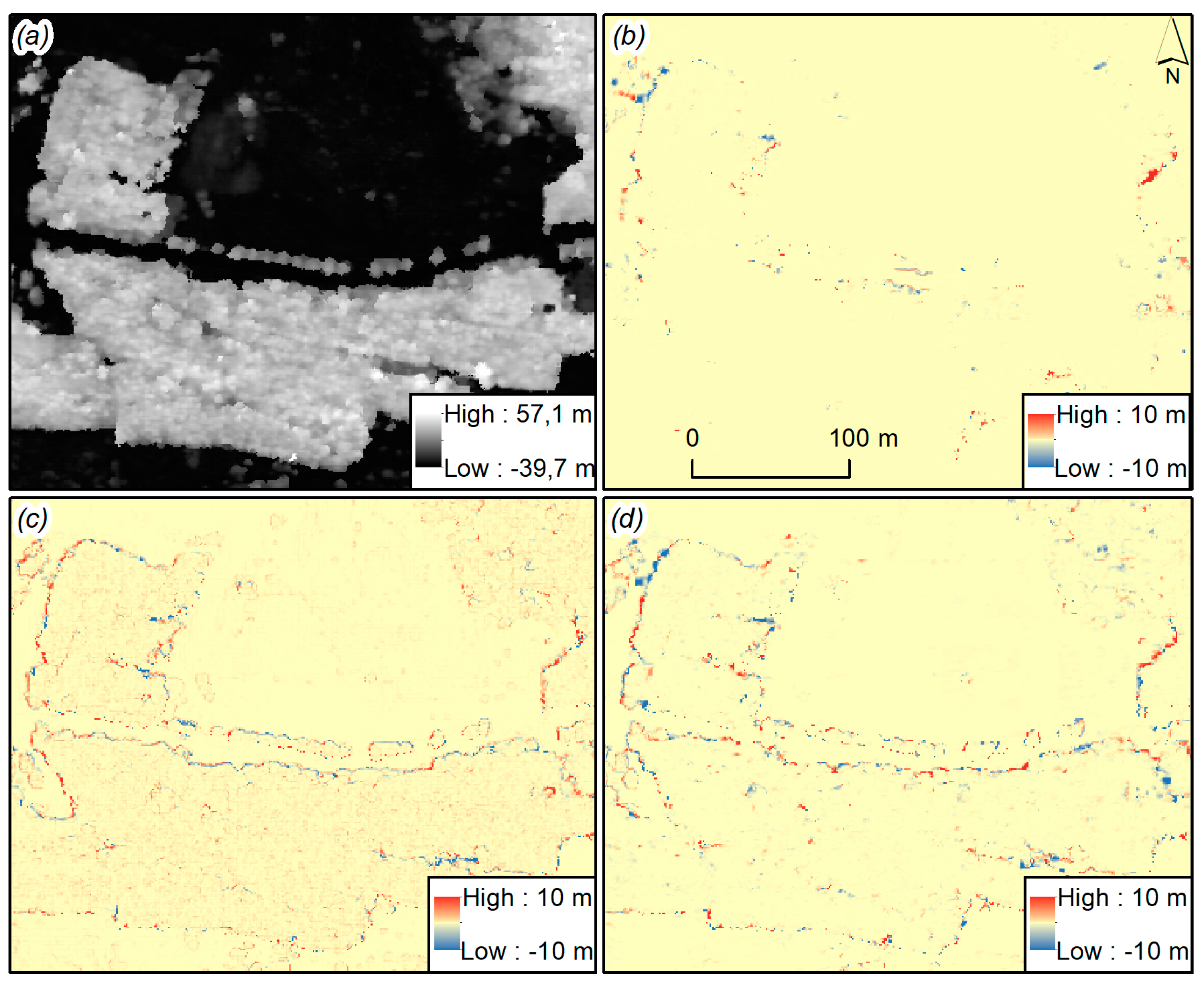
The impact of selected control parameters was analysed by comparing the following parameters: the number of filtered 3D points, time per generated DSM post, RMS (Root Mean Square) difference (Z) for the control used and adjusted points, estimated internal height accuracy (DSM), and elapsed time for DSM generation. The vertical accuracy did not change significantly regardless of the selected variant. A very large difference was visible in the density of the cloud, where variant w3 had, on average, 9 times more points than w1, w2, or w5, providing a point cloud density theoretically equal to one point per GSD value compared to other variants with image matching every 2, 3, or 5 pixels. This, of course, had an impact on the time needed to generate the cloud, but this was not a large enough effect to consider important. In this research, it was more important to be able to obtain a higher DSM accuracy. Additionally, in order to compare the impact of selecting the cloud parameters on the resulting DSM simply, images generated from different point clouds were subtracted from each other. This way, images of the differences between generated products were obtained.

The analysis of these images (Figure 6) revealed that small differences in the selection of parameters result in significant changes in the resulting cloud obtained and thus in the final rasters.

Changing only the value of parallax (pair w2–w1) resulted mainly in point differences at the boundaries of high objects due to the mapping of an object or lack thereof. Changing the level of smoothing (w5–w1) and cloud density (w3–w1) affects the contours of objects, which differ as a result of smoothing. This effect is caused by stronger interpolation, while in case of cloud condensing, objects grow their perimeters. This increases the probability of tree detection as the cloud is denser and the crown has a larger area. This visual analysis confirms the choice of w3 as the best option when generating a cloud from images in Trimble Inpho software with low smoothing and the densest point cloud generated for points found for each corresponding pixel.

4.2. The Accuracy Assessment of the DSMs Obtained using Dense Image Matching Technique

Table 4. The accuracy assessment of the height obtained based on archival photos using the dense image matching (DIM) technique (versus stereo measurements). Shades of red indicate positive values, shades of blue indicate negative values.

Date	11.08.1971			31.05.1982			30.05.1996			25.05.2003			26–29.04.2009			25.03.2012			08.08.2015			2016 field campaign
Scale/GSD	1:18,000			1:32,000			1:26,000			1:13,000			1:14,000			24 cm			25 cm
Type of photo	B/W			B/W			RGB			B/W			RGB			RGB			RGB
ID	STEREO	DIM	Δ	STEREO	DIM	Δ	STEREO	DIM	Δ	STEREO	DIM	Δ	STEREO	DIM	Δ	STEREO	DIM	Δ	STEREO	DIM	Δ	Tree Species	Hin-situ	Cdensity	Cdiameter
83	9.5	9.6	–0.1	12.7	1.2	11.5	13.8	1.2	12.6	15.4	16.7	–1.3	16.5	0.9	15.6	17.6	2.5	15.1	17.7	17.2	0.5	Acer platanoides	20.0	60	15
136	11.4	8.8	2.6	13.0	3.0	10.0	14.3	0.9	13.4	16.2	16.4	–0.2	16.9	13.5	3.4	17.1	2.2	14.9	17.6	17.1	0.5	Acer platanoides	17.0	80	15
67	6.4	3.3	3.1	8.1	1.1	7.0	9.2	1.5	7.7	9.5	10.5	–1.0	10.4	10.1	0.3	11.0	0.5	10.5	12.3	12.3	0.0	Acer platanoides	15.0	90	6
135	9.7	9.7	0.0	11.0	0.2	10.8	12.0	4.5	7.5	12.9	14.1	–1.2	13.0	12.8	0.2	13.4	4.5	8.9	14.1	13.0	1.1	Acer platanoides	15.0	60	15
21	7.5	1.6	5.9	8.4	2.0	6.4	12.8	6.8	6.0	15.2	14.7	0.5	17.2	3.0	14.2	16.4	0.7	15.7	17.4	17.5	–0.1	Acer saccharum	18.0	60	10
32	11.5	13.2	–1.7	13.3	14.8	–1.5	15.1	9.4	5.7	16.6	17.0	–0.4	17.2	17.3	–0.1	17.9	11.4	6.5	17.7	17.4	0.3	Aesculus hippocastanum	20.0	90	2+4
4	2.5	3.4	–0.9	3.8	1.6	2.2	7.3	6.6	0.7	7.7	7.2	0.5	9.9	8.7	1.2	11.2	9.9	1.3	12.7	11.7	1.0	Betula pendula	13.0	60	6
65	7.1	7.7	–0.6	8.0	5.9	2.1	10.5	1.6	8.9	11.4	12.1	–0.7	12.2	6.0	6.2	12.2	1.5	10.7	13.5	12.9	0.6	Carpinus betulus	15.5	90	12
31	3.5	0.1	3.4	4.6	1.5	3.1	5.0	4.8	0.2	5.3	8.6	–3.3	5.7	6.0	–0.3	6.4	2.3	4.1	7.5	7.7	–0.2	Corylus avellana	9.0	90	10
33	3.4	–0.5	3.9	4.2	3.6	0.6	5.3	1.3	4.0	6.3	6.6	–0.3	6.8	6.0	0.8	6.7	1.7	5.0	9.7	8.7	1.0	Crataegus monogyna	8.0	90	8
88	4.1	1.7	2.4	4.4	4.4	0.0	4.6	6.0	–1.4	4.7	4.1	0.6	4.5	0.7	3.8	4.9	1.1	3.8	4.6	3.6	1.0	Crataegus monogyna	4.5	90	4
54	8.0	9.3	–1.3	9.2	1.4	7.8	11.6	13.1	–1.5	12.9	13.3	–0.4	13.1	0.3	12.8	14.7	2.3	12.4	15.0	14.2	0.8	Fraxinus excelsior	16.0	50	2+5
102	3.9	1.4	2.5	5.1	1.0	4.1	7.3	1.6	5.7	7.8	7.7	0.1	8.4	0.0	8.4	8.6	0.8	7.8	9.5	10.0	–0.5	Fraxinus excelsior	12.0	30	10
2	4.4	6.3	–1.9	6.3	3.4	2.9	10.3	5.2	5.1	9.6	10.2	–0.6	9.9	0.1	9.8	11.1	1.6	9.5	12.2	10.5	1.7	Fraxinus excelsior	14.0	10	7
109	6.1	0.4	5.7	6.7	0.8	5.9	7.5	3.7	3.8	7.1	8.5	–1.4	7.6	6.6	1.0	6.6	5.9	0.7	7.7	7.4	0.3	Malus domestica	7.5	80	11
13	10.9	11.1	–0.2	12.2	10.6	1.6	13.9	6.1	7.8	14.1	13.1	1.0	14.9	12.3	2.6	15.7	15.1	0.6	15.4	14.6	0.8	Pinus sylvestris	15.0	60	4+1
14	8.3	9.1	–0.8	9.1	8.9	0.2	10.4	6.8	3.6	12.4	11.7	0.7	14.1	9.7	4.4	15.0	14.7	0.3	15.0	14.8	0.2	Pinus sylvestris	14.5	70	9
3	10.0	11.1	–1.1	11.4	10.8	0.6	14.3	5.6	8.7	14.2	15.5	–1.3	14.5	14.4	0.1	15.0	14.9	0.1	15.1	14.7	0.4	Pinus sylvestris	13.0	70	8
15	9.9	14.5	–4.6	11.2	0.9	10.3	12.8	2.3	10.5	13.2	1.1	12.1	13.7	4.9	8.8	14.2	13.6	0.6	14.1	13.8	0.3	Pinus sylvestris	13.0	70	4+1
8	6.1	6.2	–0.1	7.0	1.6	5.4	7.7	6.3	1.4	8.0	6.8	1.2	8.4	0.4	8.0	8.3	7.6	0.7	8.5	8.3	0.2	Pinus sylvestris	12.0	70	5
10	4.9	6.4	–1.5	6.1	2.9	3.2	6.8	6.3	0.5	7.0	7.2	–0.2	7.0	0.5	6.5	7.1	7.0	0.1	7.6	7.2	0.4	Pinus sylvestris	12.0	70	6
12	6.5	6.2	0.3	8.7	1.6	7.1	9.2	8.8	0.4	9.5	9.6	–0.1	9.8	9.1	0.7	9.7	10.6	–0.9	9.8	9.5	0.3	Pinus sylvestris	12.0	70	6
22	6.2	5.9	0.3	7.2	1.8	5.4	7.5	1.4	6.1	8.1	9.7	–1.6	8.5	8.5	0.0	9.5	7.1	2.4	10.3	10.1	0.2	Pinus sylvestris	12.0	70	9
5	4.8	5.1	–0.3	6.2	6.0	0.2	7.7	3.9	3.8	8.2	7.8	0.4	9.2	5.7	3.5	8.2	7.1	1.1	9.1	8.6	0.5	Pinus sylvestris	12.0	50	5+1
9	6.8	7.9	–1.1	8.5	1.1	7.4	9.3	9.1	0.2	9.2	9.2	0.0	9.5	9.1	0.4	9.8	8.9	0.9	9.9	9.7	0.2	Pinus sylvestris	11.0	70	6
11	8.0	7.6	0.4	9.6	1.1	8.5	11.4	9.6	1.8	11.8	12.5	–0.7	12.0	10.2	1.8	12.1	10.1	2.0	12.2	12.0	0.2	Pinus sylvestris	11.0	70	6
94	6.2	4.0	2.2	10.3	5.5	4.8	14.0	13.8	0.2	16.3	9.8	6.5	17.6	0.6	17.0	19.8	4.2	15.6	19.5	18.5	1.0	Populus balsamifera	25.0	60	13
95	6.5	4.1	2.4	11.8	13.1	–1.3	14.3	12.4	1.9	15.4	15.5	–0.1	17.0	5.8	11.2	20.7	4.9	15.8	20.0	11.8	8.2	Populus balsamifera	25.0	10	15
1	2.6	1.0	1.6	5.2	3.2	2.0	6.8	1.7	5.1	8.9	9.1	–0.2	9.3	0.7	8.6	10.4	1.5	8.9	11.7	11.2	0.5	Pyrus communis	16.0	70	9
45	6.1	1.1	5.0	7.7	1.9	5.8	7.6	0.5	7.1	7.7	8.0	–0.3	8.3	8.3	0.0	9.1	4.8	4.3	10.1	9.0	1.1	Pyrus communis	12.0	90	5
132	7.4	8.3	–0.9	8.7	2.2	6.5	8.9	2.2	6.7	9.9	9.8	0.1	9.8	9.4	0.4	10.6	6.5	4.1	11.3	10.4	0.9	Pyrus communis	12.0	70	9
68	3.1	3.4	–0.3	4.6	0.5	4.1	6.3	2.7	3.6	8.0	8.9	–0.9	8.5	8.3	0.2	8.8	6.8	2.0	9.7	8.6	1.1	Pyrus communis	10.0	80	9
34	6.8	2.0	4.8	6.8	1.4	5.4	6.8	6.0	0.8	6.9	7.8	–0.9	7.4	7.2	0.2	7.6	1.0	6.6	8.3	7.5	0.8	Pyrus communis	10.0	70	6
35	2.7	3.1	–0.4	4.8	0.8	4.0	6.7	5.5	1.2	8.5	8.6	–0.1	8.9	4.8	4.1	8.9	7.3	1.6	9.5	8.9	0.6	Pyrus communis	10.0	70	7
30	6.0	2.1	3.9	6.1	1.4	4.7	6.5	6.6	–0.1	7.0	7.7	–0.7	7.3	7.1	0.2	7.5	4.8	2.7	7.5	7.1	0.4	Pyrus communis	10.0	50	8
41	3.7	2.1	1.6	4.2	1.2	3.0	5.6	0.9	4.7	5.6	4.4	1.2	6.4	0.2	6.2	8.6	0.5	8.1	10.2	9.4	0.8	Quercus robur	13.0	20	4
28	5.3	3.9	1.4	7.3	1.6	5.7	10.3	4.4	5.9	12.2	10.4	1.8	14.5	0.3	14.2	14.9	1.6	13.3	14.8	12.6	2.2	Robinia pseudoacacia	16.0	10	8
87	5.6	3.6	2.0	7.6	0.9	6.7	9.8	1.6	8.2	11.0	14.0	–3.0	13.0	0.7	12.3	14.3	8.6	5.7	14.7	14.0	0.7	Salix fragilis	16.0	40	11
27	7.8	10.7	–2.9	8.0	1.6	6.4	8.4	2.6	5.8	9.2	10.9	–1.7	9.7	0.4	9.3	10.9	2.5	8.4	11.6	10.7	0.9	Salix fragilis	14.0	20	12
44	3.7	3.5	0.2	4.9	1.6	3.3	7.6	3.1	4.5	7.2	6.7	0.5	8.2	8.7	–0.5	9.9	4.5	5.4	11.8	11.2	0.6	Salix fragilis	12.0	30	10
19	20.0	20.1	–0.1	20.3	24.6	–4.3	20.6	25.4	–4.8	21.5	25.7	–4.2	21.6	4.8	16.8	22.9	1.1	21.8	22.9	22.2	0.7	Tilia platyphyllos	25.0	90	9
66	11.8	8.1	3.7	13.5	14.3	–0.8	17.2	11.5	5.7	18.4	11.0	7.4	19.5	18.8	0.7	19.7	10.1	9.6	20.3	20.0	0.3	Tilia platyphyllos	25.0	90	15
all species:		sD =	2.37		sD =	3.57		sD =	3.88		sD =	2.74		sD =	5.49		sD =	5.65		sD =	1.27
deciduous:		sD =	2.36		sD =	3.62		sD =	4.01		sD =	2.26		sD =	6.02		sD =	5.23		sD =	1.45
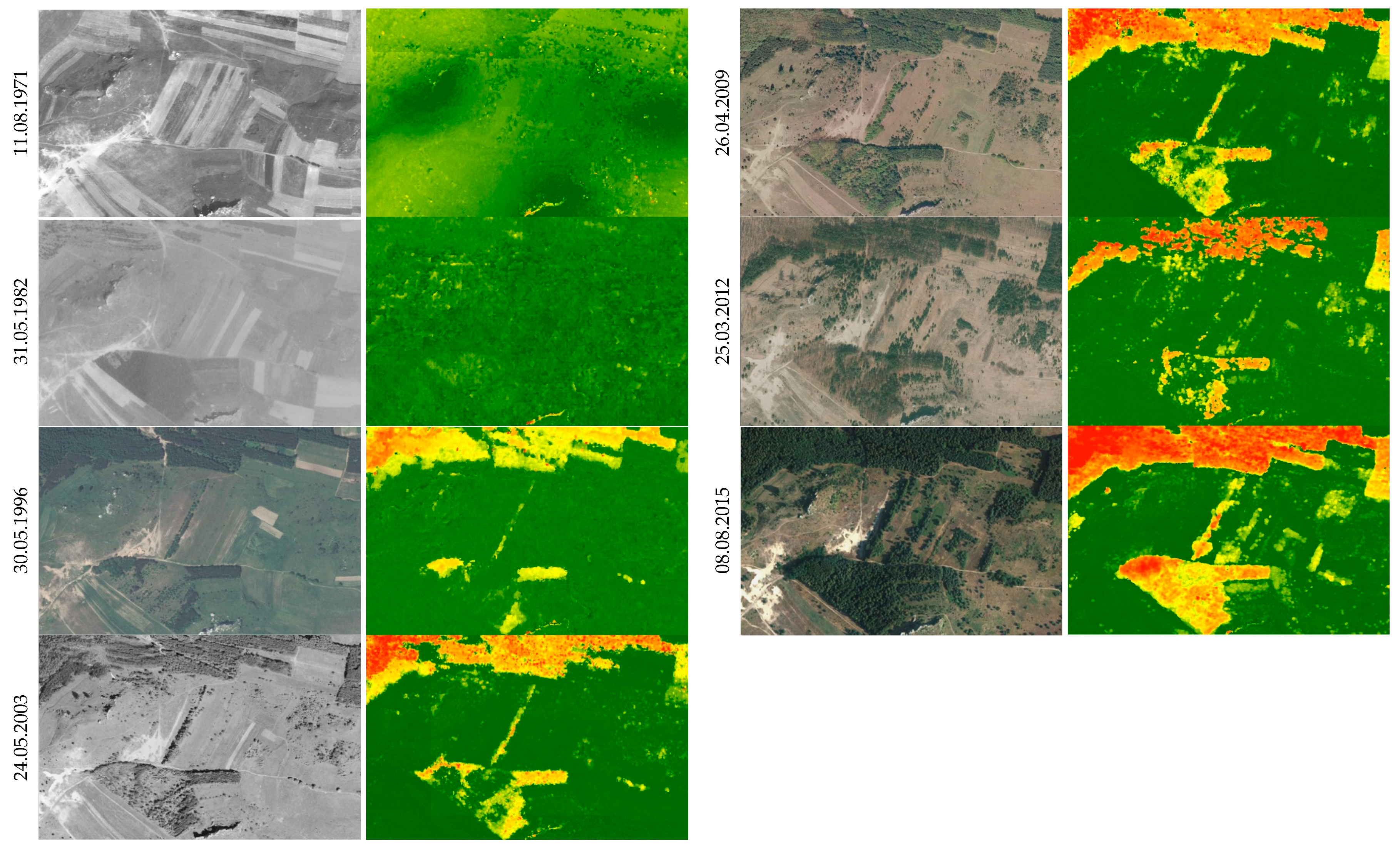
coniferous:		sD =	1.40		sD =	3.59		sD =	3.66		sD =	3.79		sD =	3.21		sD =	0.89		sD =	0.19

presents the accuracy assessment of the heights obtained based on archival photographs using dense image matching techniques versus stereo measurements. The visual presentation of these results is shown in Figure 7. The highest accuracy was obtained with the DSM from 2015, which was created from digital colour images of the best radiometric and geometric quality (GSD = 25 cm). These aerial photos were collected during the fully developed growing season; therefore, all species of trees and shrubs were visualised correctly. The standard deviation of the height difference determined by both methods equals 1.27 m (Table 4). Analysing the differences obtained for particular species, it was noticed that conifer species are relatively small (generally 0.2–0.4 m, standard deviation of the height difference determined by both methods is 0.19 m), while for deciduous species the variation is much higher (standard deviation of the difference in height determined by both methods is 1.45 m, 0.54 after eliminating Populus balsamifera with 10% crown density). The largest differences in height were observed for individuals with open canopy closure (10%–20% of height). Analysing the data from 2015, it can be noticed that the size and the closure of its crown have a notable impact on the accuracy of the tree heights obtained using the DIM algorithm. In the case of less dense crowns, the contrast between the crown and its surroundings significantly affects the operation of DIM algorithms.

The least accurate results were obtained based on aerial photographs from 2012, 2009, 1996, and 1982. In 2012 and 2009, this was caused by the image acquisition date (March and April), which was at the beginning of the growing season in Poland when most of the trees and shrubs were still leafless or in the early stages of development. This issue limited the effective detection of trees and shrubs. Most values of Δ are positive, which means that these trees in DSM were not contained with their height. Only in the case of coniferous trees was high accuracy obtained for most individuals (problems only occur in the case of pines with irregular crowns). The R² coefficient for coniferous trees was for 1971: 0.51, 1996: 0.36, 2003: 0.89, 2009: 0.64, 2012: 0.93, and 2015: 0.99.

Aerial photographs from 1996 and 1982 were made in smaller scales, 1:26,000 and 1:32,000, respectively, which lowered the accuracy of the DSMs generated, for both deciduous and coniferous species. The standard deviation of the height differences is 3.57 m for 1982 and 3.88 m for 1996 (Table 4). In both these terms, significant outliers (up to 13 m) can be observed for a few individuals. 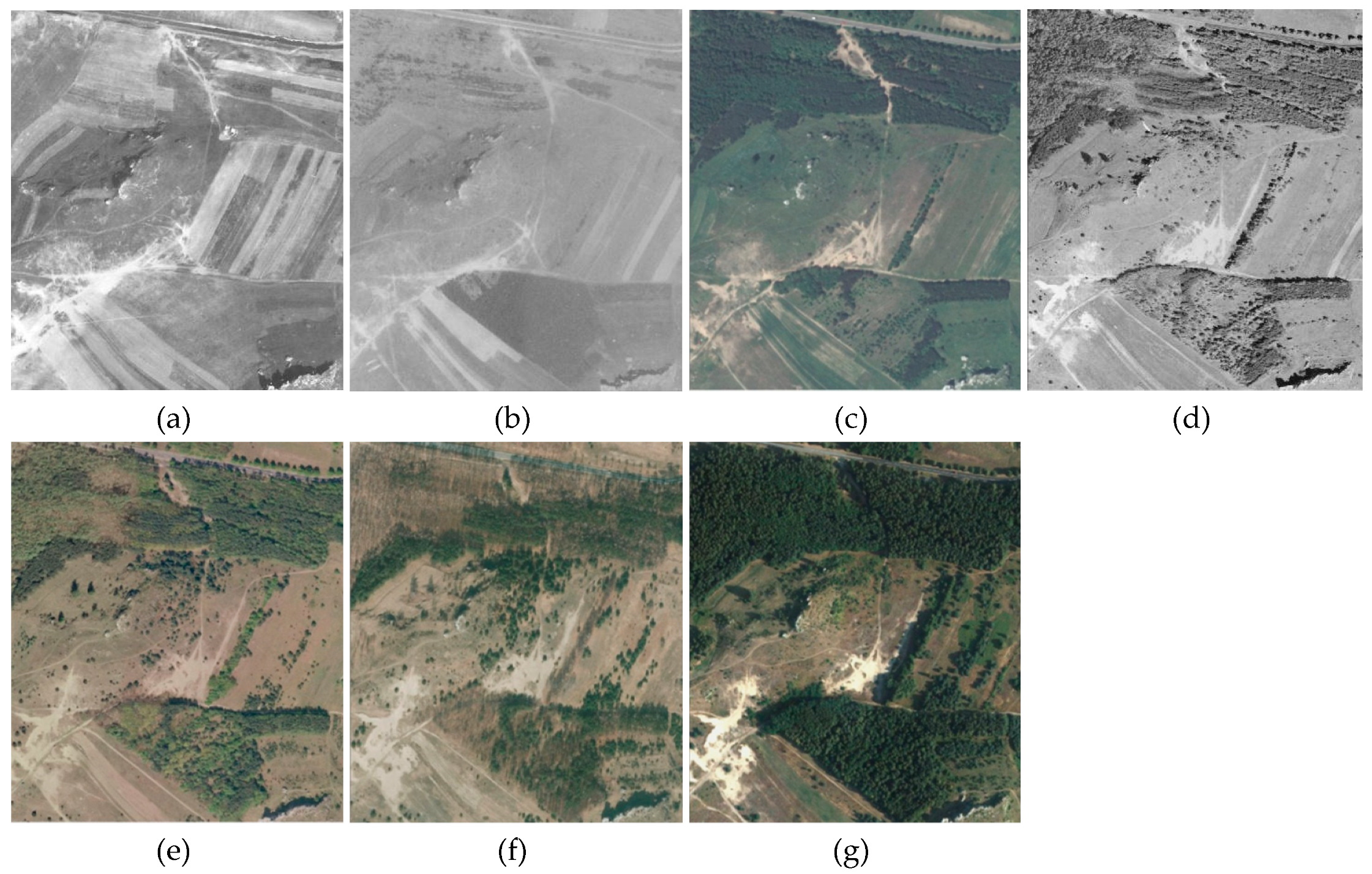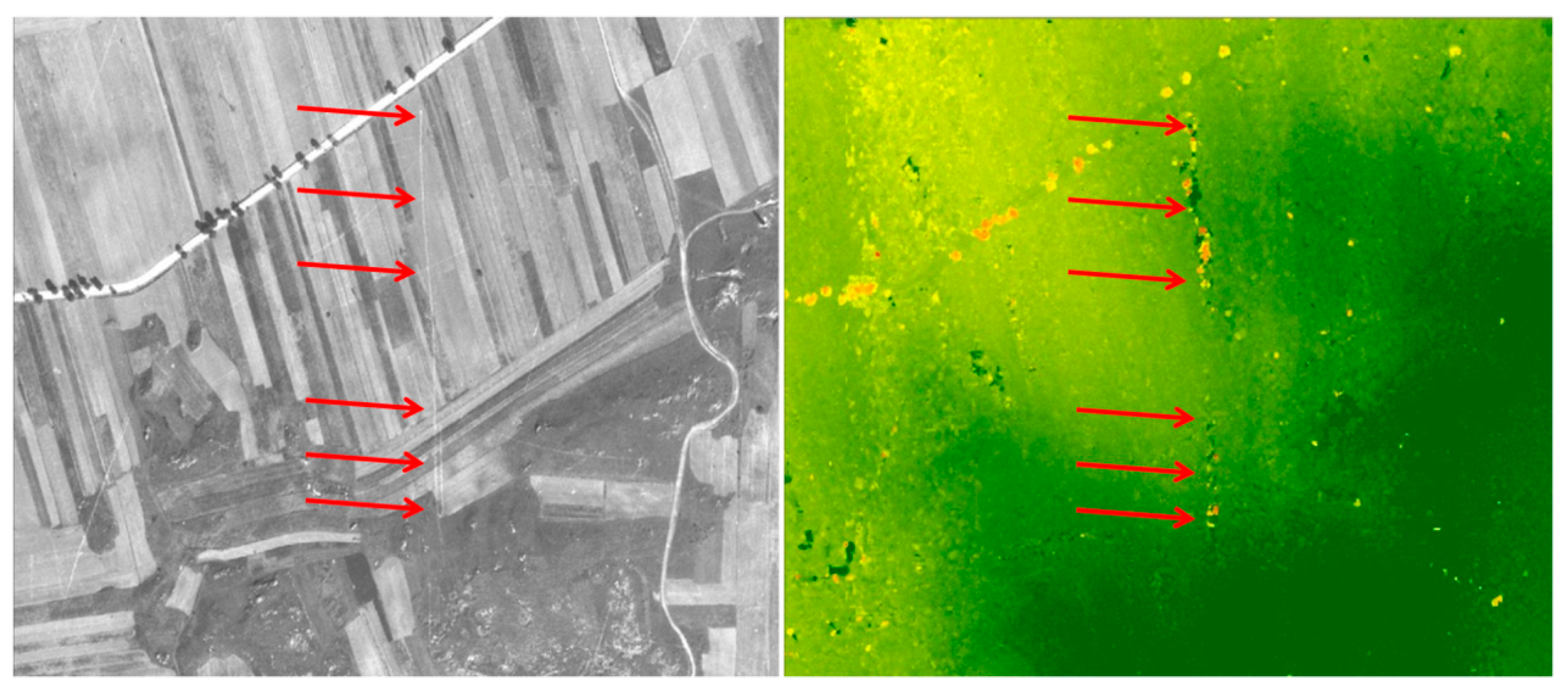This applies particularly to deciduous trees (the biggest errors were obtained for Acer spp.). For photographs from 1971 and 1982, the poor radiometric quality and visible film damage (Figure 8) caused significant errors in the elevation model.

Summing up the performed accuracy analysis, the DSMs with the highest accuracy were obtained using images acquired in the fully developed growing season, with a scale of at least 1:13,000 (analogue cameras) or with a GSD less than or equal to 25 cm (digital cameras).

4.3. Analysis of the Effectiveness of the Tree and Shrub Detection using DIM

In order to evaluate the effectiveness of the DIM technique with respect to its use in the analysis of the succession process dynamics, an experiment with multitemporal data, various acquisition terms, and varied image qualities was carried out to determine what features of the examined objects affect the results of their detection. These analyses were conducted for nDSMs obtained using aerial photos from 2015 because the date of their acquisition was the nearest to the date of the field botanical campaigns (2016–2017) and the registration date of ALS data (2016). In addition, aerial photos from 2015 were acquired during the growing season, with GSD = 25 cm, therefore producing the best parameters from the analysed set of archival data.

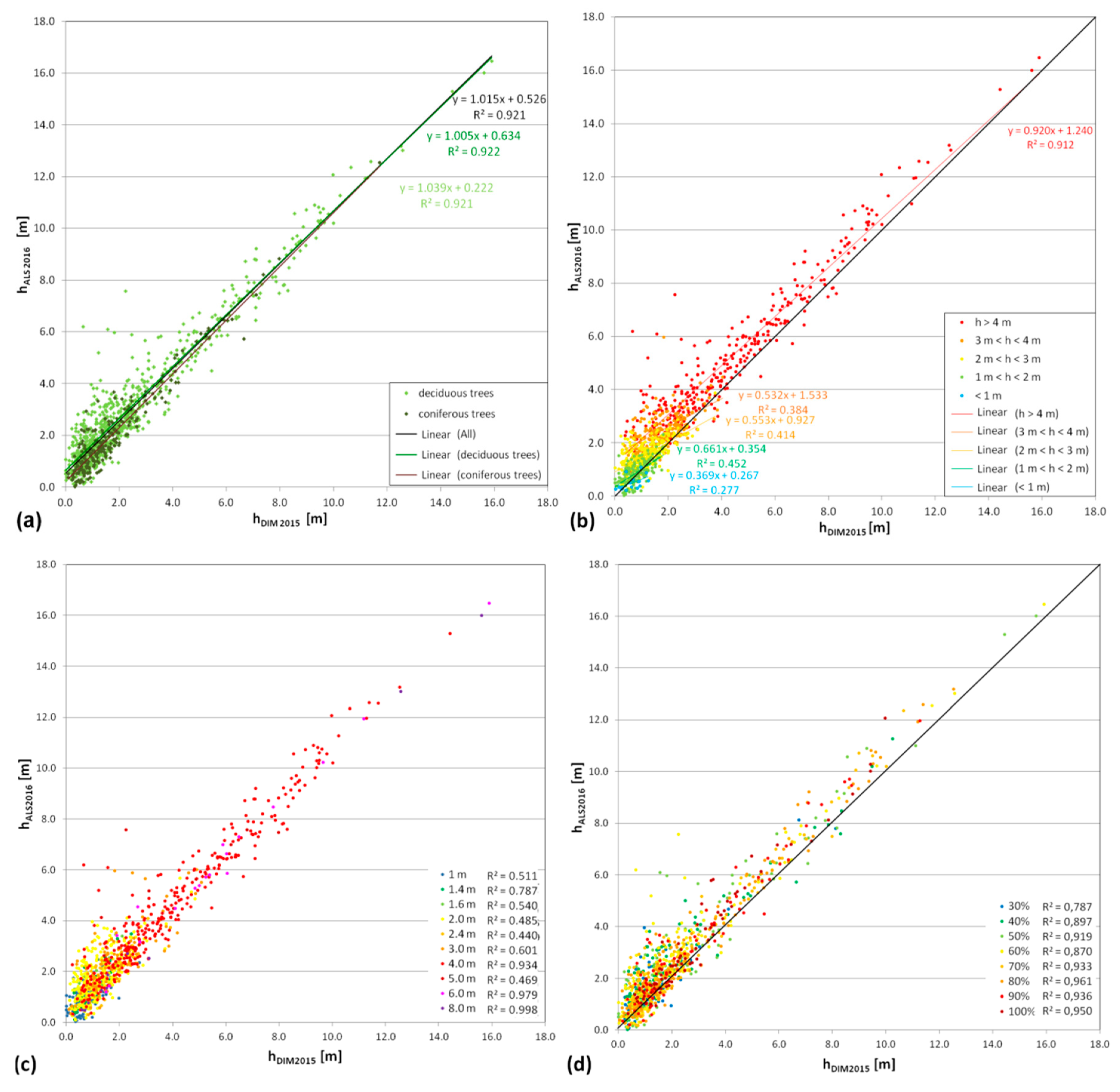
The effectiveness analysis included an impact analysis of the parameters of trees and shrubs (height, crown diameter, crown density) on the tree and shrub detection using the DIM technique. The comparison of the height of trees and shrubs obtained based on ALS data and as a result of DIM techniques depending on the species, height, size, and crown density of the examined trees and shrubs are presented in

Table 5. Mean differences between the height of the trees and shrubs obtained using airborne laser scanning (ALS) (2016–reference data) and DIM (2015) taking into account the tree and shrub species.

Tree and Shrubs Species	μ|ΔALS-DIM| [m]
All	0.66
Coniferous	0.43
Juniperus communis	0.34
Pinus sylvestris	0.58
Deciduous	0.73
Deciduous trees	0.85
Betula pendula	1.02
Fraxinus sp.	1.64
Padus serotina	0.67
Populus tremula	1.19
Pyrus communis	0.88
Quercus robur	0.81
Quercus rubra	1.07
Robinia pseudoacacia	1.11
Deciduous shrubs	0.49
Cornus sanguinea	0.43
Corylus avellana	0.81
Crataegus sp.	0.57
Frangula alnus	0.40
Ligustrum vulgare	0.41
Prunus spinosa	0.38
Rhamnus cathartica	0.46
Rosa canina	0.37

,

Table 6. Mean differences between the height of the trees and shrubs obtained using ALS (2016–reference data) and DIM (2015) considering the height of trees and shrubs.

Height [m]	All Species		Coniferous		Deciduous
	μ|ALS-DIM| [m]	μ|ALS-DIM|/ hmean	μ|ALS-DIM| [m]	μ|ALS-DIM|/ hmean	μ|ALS-DIM| [m]	μ|ALS-DIM|/ hmean
>12.0	0.92	7.65%	0.82	6.83%	0.98	8.15%
10.0–12.0	0.93	9.31%	0.39	3.87%	0.98	9.80%
9.0–10.0	0.67	7.45%	0.27	2.99%	0.68	7.60%
8.0–9.0	0.73	9.18%	-	-	0.73	9.18%
7.0–8.0	1.05	14.94%	0.63	9.02%	1.17	16.71%
6.0–7.0	1.04	17.32%	0.68	11.40%	1.10	18.30%
5.0–6.0	1.10	22.00%	0.68	13.63%	1.18	23.68%
4.0–5.0	0.86	21.59%	0.53	13.20%	0.94	23.54%
3.0–4.0	0.77	25.66%	0.72	24.16%	0.78	25.98%
2.0–3.0	0.51	25.53%	0.38	18.91%	0.56	27.99%
1.5–2.0	0.28	18.36%	0.23	15.39%	0.30	20.12%
1.0–1.5	0.26	26.14%	0.21	21.01%	0.30	29.81%
<1.0	0.28	28.37%	0.39	39.35%	0.22	21.78%

,

Table 7. Mean differences between the height of the trees and shrubs obtained using ALS (2016–reference data) and DIM (2015) considering the crown diameter.

Crown Diameter [m]	All Species	Coniferous	Deciduous
	μ|ALS-DIM| [m]	μ|ALS-DIM| [m]	μ|ALS-DIM| [m]
8.00	0.27	-	0.27
6.00	0.59	0.27	0.65
5.00	1.27	-	1.27
4.00	0.74	0.52	0.78
3.00	0.71	0.28	0.81
2.40	0.71	0.75	0.70
2.00	0.67	0.40	0.77
1.60	0.65	0.78	0.55
1.40	0.43	0.52	0.40
1.00	0.40	0.35	0.44

and

Table 8. Mean differences between the height of the trees and shrubs obtained using ALS (2016–reference data) and DIM (2015) considering the crown density.

Crown Density [%]	All Species	Coniferous	Deciduous
	μ|ALS-DIM| [m]	μ|ALS-DIM| [m]	μ|ALS-DIM| [m]
100	0.57	0.39	0.64
90	0.64	0.42	0.75
80	0.61	0.41	0.69
70	0.62	0.44	0.70
60	0.74	0.45	0.82
50	0.70	0.41	0.77
40	0.71	0.64	0.72
30	0.59	0.41	0.63

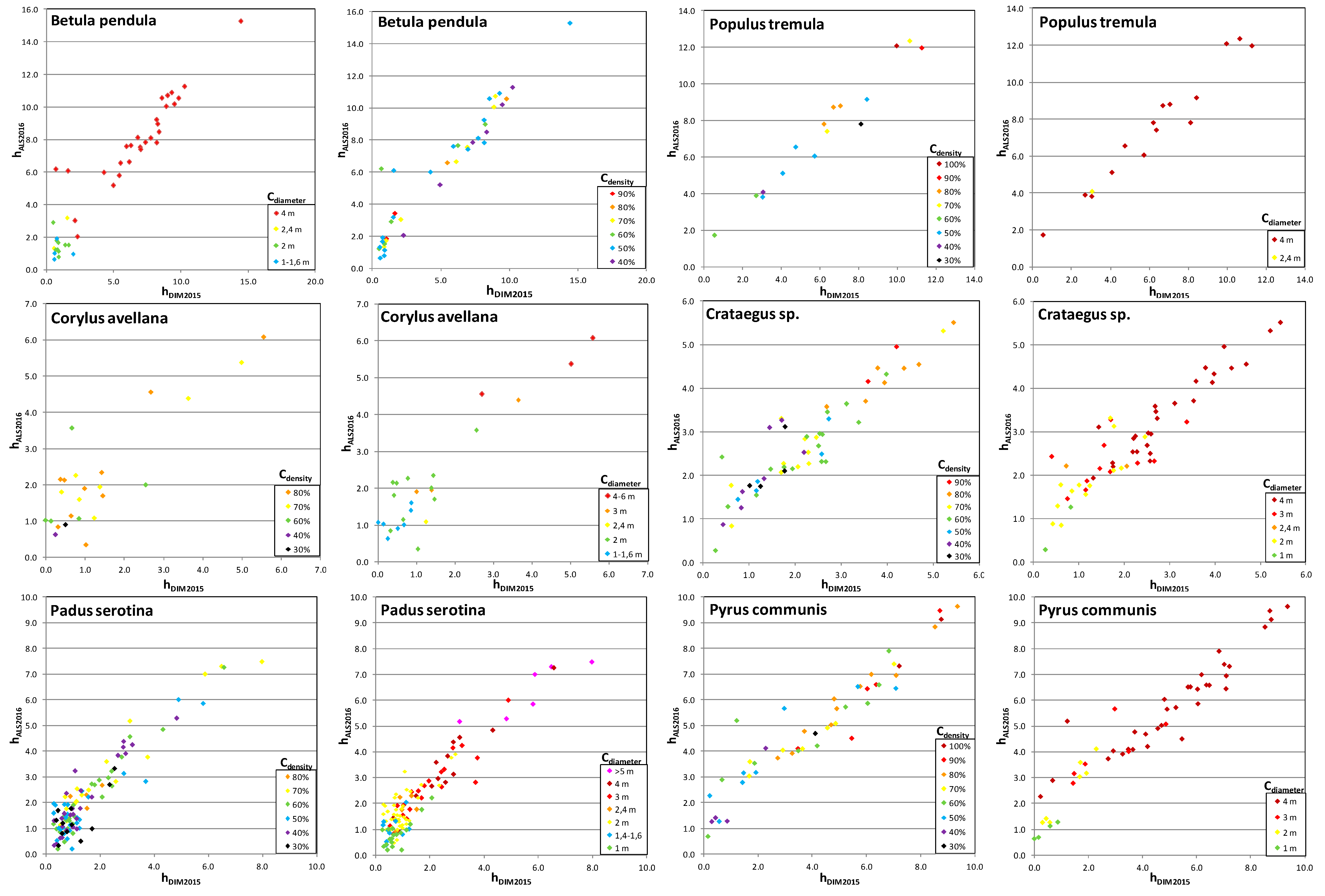
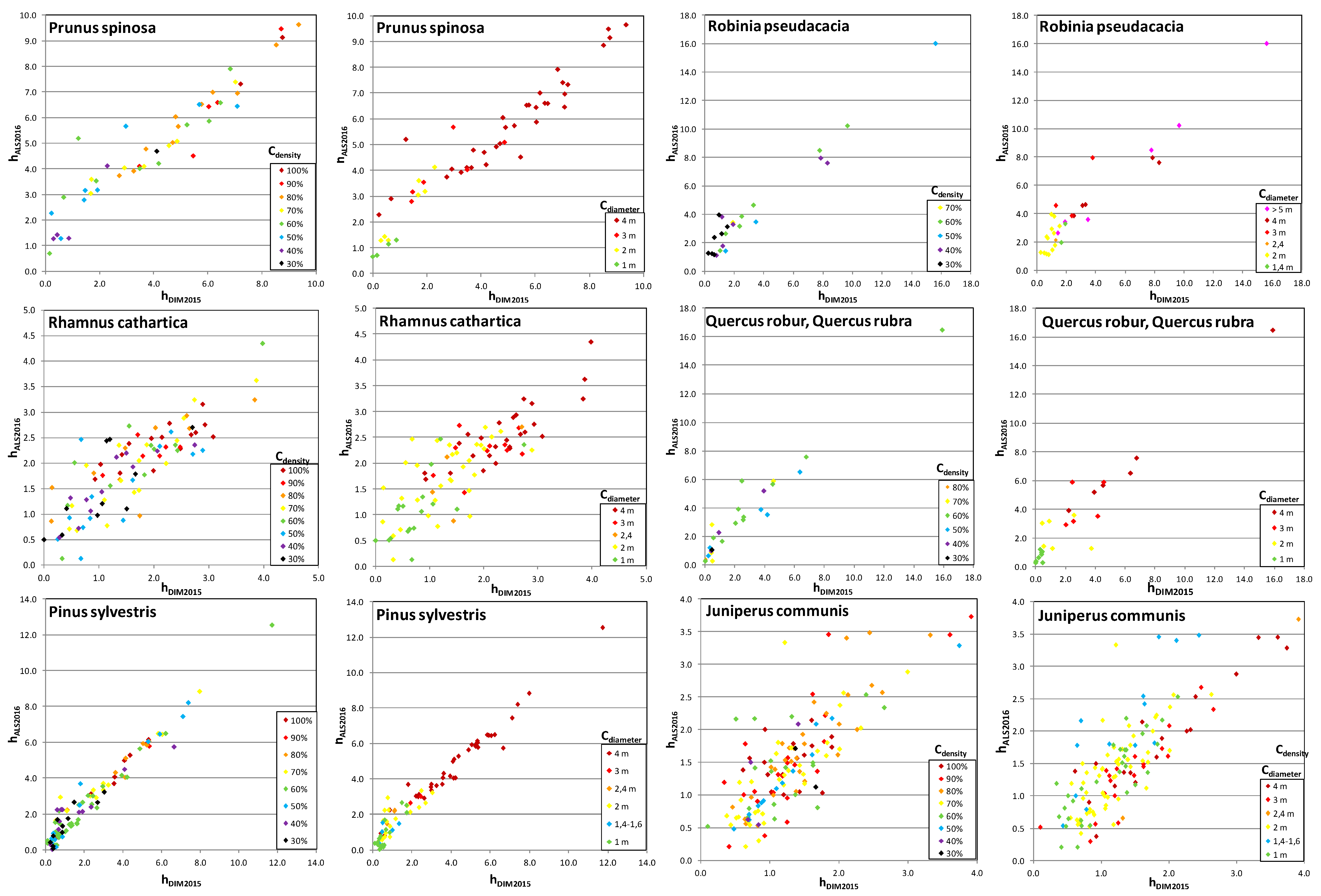
, and in the sub-figures in Figure 9. The influence of crown diameter and density (by species) on the accuracy of the height of trees and shrubs using DIM techniques are illustrated in Figure 10.

The height differences indicate that a higher accuracy for determining the height of trees and shrubs is acquired for conifers (Table 5, μ_|ΔALS-DIM| = 0.43 m). In the case of deciduous trees and shrubs, the mean value of height differences is 0.73 m; it is strongly differentiated (from 0.37 m to 1.64 m, and μ_|ΔALS-DIM| = 0.73 m) and depends on the species and size of the measured object. In general, it was found that tree species, especially those with loose crowns (Betula pendula, Populus tremula), were characterized by higher values of height differences (Figure 10). In the case of Fraxinus sp., Robinia pseudoacacia, and Quercus rubra, larger differences arise from the specifics of objects present in the study area—some of them were characterized by a small crown density (30%–50%) (Robinia pseudoacacia) or smaller crown diameter (Figure 10), moreover Fraxinus sp. and Quercus rubra did not occur in large numbers.

Shrubs are characterized by a much smaller error in determining the height than is the case for woody species (the exception here is Corylus avellana). This applies to both deciduous and coniferous shrubs (Juniperus communis). The average height differences of shrubs obtained based on LIDAR data and using DIM techniques are 0.49 m for deciduous shrubs and 0.34 m for coniferous, respectively. However, considering their lower heights compared to woody species, the relative error of determining the height is quite high, because it reaches 20%–28% of the height of the shrub (Table 6). In the case of trees, this error is generally less than 16%.

Analysing the effect of object features on the accuracy of the tree and shrub detection, greater variation in the height difference, μ_|ALS-DIM|, occurs in deciduous trees and increases with decreasing tree height and reducing crown density (Figure 9a–d). Coniferous trees are generally characterized by a better height mapping than is the case for deciduous trees (Table 5, Figure 9a). It can also be noticed that the larger the tree crown (diameter over 3–4 m), the better the height mapping using DIM techniques (Figure 9c). The graphs in Figure 9 show outliers that represent deciduous trees with a height of approx. 5–6 m. These are Betula pendula, Fraxinus sp., and Quercus rubra with tree crowns with 3–4 meter diameters and 50%–60% density (Figure 9c,d). Betula pendula is common in the analysed area. During the secondary succession process, Betula pendula enters abandoned fields and unused grasslands as one of the first tree species. Most individuals have well-developed, slender crowns. Over a dozen-year-olds, medium height individuals of Betula pendula dominate, which is associated with the massive abandonment of cultivation and grazing over the last 20 years.

Fraxinus sp. and Quercus rubra are rarely found in the analysed area. Fraxinus sp. is usually planted as a roadside tree, Quercus rubra grows spontaneously in abandoned fields and grasslands, and sometimes is planted in forests. Most individuals of both Fraxinus sp. and Quercus rubra growing in abandoned fields and grasslands have well-developed, spherical crowns. But individuals of Fraxinus sp. are usually adult, and individuals of Quercus rubra are mostly young.

Analysis of the similarity degree of heights obtained based on LIDAR data from 2016 and using DIM algorithms (Figure 9c), depending on the size of crowns, showed that trees and shrubs with a crown size above 4 m are characterized by the highest compatibility of both heights (R² above 0.9, with the exception of 5 m crown diameter, which is due to the small sample number of such objects).

Analysing the influence of species on the results, for smaller shrubs and brushwood (with a crown diameter less than 2.4 m (Table 7) and height less than 2 m (Table 6)), there was no influence of type, species, or other traits on the value of μ_|ALS-DIM|. Both coniferous and deciduous species are at a similar level. For larger trees, μ_|ALS-DIM| values are reduced for coniferous species. No influence was observed for the density of crowns of trees and shrubs on the obtained mean differences in height, μ_|ALS-DIM (Table 8). Because the analysed area has physiognomically different grades with different heights and crowns, an analysis was carried out with differences in height depending on: heights and crown diameters (

Table 9. Mean differences between the height of the deciduous trees and shrubs obtained using ALS (2016–reference data) and DIM (2015) considering the tree height and crown diameter.

		Crown Diameter [m]
		5.0–8.0	4.0	3.0	2.4–2.6	2.0	1.4–1.6	1
Height [m]	>10	0.47	1.10	-	-	-	-	-
	8–10	0.71	0.90	-	-	-	-	-
	6–8	1.42	0.87	1.10	-	-	-	-
	4–6	1.08	0.86	1.54	1.01	0.92	-	-
	2–4	0.65	0.65	0.77	0.75	1.07	1.01	0.60
	1–2	0.20	0.42	0.45	0.51	0.53	0.49	0.49
	<1.0	0.13	0.24	0.36	0.40	0.26	0.22	0.28

), heights and crown density (

Table 10. Mean differences [m] between the height of the deciduous trees and shrubs obtained using ALS (2016–reference data) and DIM (2015) considering the tree height and crown density.

		Crown Density [%]
		100	90	80	70	60	50	40	30
Height [m]	>10	1.19	0.69	0.94	1.18	0.60	1.00	0.87	-
	8–10	0.42	1.15	1.08	0.81	0.72	0.75	0.42	1.38
	6–8	0.92	0.88	0.69	0.66	1.74	1.03	0.52	0.85
	4–6	1.04	0.55	0.62	0.72	1.14	1.53	1.07	1.78
	2–4	0.57	0.85	0.75	0.82	0.83	0.83	1.09	1.01
	1–2	0.34	0.41	0.43	0.48	0.57	0.56	0.60	0.48
	<1.0	0.37	0.28	0.30	0.24	0.27	0.27	0.66	0.34

), crown diameter and density (

Table 11. Mean differences [m] between the height of the deciduous trees and shrubs obtained using ALS (2016–reference data) and DIM (2015) considering the crown diameter and density.

		Crown Density [%]
		100	90	80	70	60	50	40	30
Crown diameter [m]	5.0–8.0	-	-	0.63	0.83	1.19	0.26	0.34	-
	4.0	0.63	0.67	0.69	0.64	1.15	0.98	0.78	0.85
	3.0	0.27	0.85	0.57	0.51	0.87	1.13	0.90	-
	2.4–2.6	-	-	0.82	0.86	-	0.78	0.69	0.75
	2.0	0.45	-	0.70	0.90	0.60	0.80	0.89	0.80
	1.4–1.6	-	-	0.66	0.57	0.52	0.30	0.53	0.44
	1.0	-	-	0.78	0.39	0.44	0.41	0.38	0.44

).

The results summarized in Table 9 indicate that the mean height differences, μ _{| ALS-DIM |}, for trees and shrubs from a certain height range slightly increase when the crown diameter of a tree or bush decreases. Only in the case of crowns with a larger diameter is there no such a clear tendency, which may result from other features, such as species or shortening of the crown. Figure 10 clearly shows that shrub species (especially Rhamnus cathartica, Juniperus communis, Crataegus spp.) are characterized by large differences in height depending on the diameter and density of the crown. For Crataegus spp., the smallest height deviations were noted for higher crown densities. The largest deviations in height for Juniperus communis were from shrubs with a smaller crown diameter (<1.6 m). The differences observed in height obtained using DIM vs. ALS results mainly from the specificity of these species and their habit.

For smaller shrubs and trees (up to a height of 2 m), there is no significant relationship between crown density and the value of μ _|ALS-DIM| (Table 10). Clear trends are visible only for trees and shrubs higher than 2 m. In most cases, for lower crown density (below 60%), differences in height with respect to ALS data are higher, but two exceptions were found here. For example, high values for trees with a height over 10 m and 100% crowns are for individuals with narrow crowns, which affects the results of the DIM algorithm.

A similar situation is seen for the analysis of the relationship between the crown diameter and crown density (Table 11). In the case of small trees and shrubs with crown diameters below 1.6 m, the influence of the crown density on the correctness of vegetation height cannot be noticed. For larger individuals with less than 60% crown density, generally higher differences with the ALS data in the value of μ_|ALS-DIM| were found. These results were confirmed with R² determination coefficients obtained to determine the degree of similarity of the heights based on the ALS data from 2016 and as a result of the DIM algorithms (Figure 9d). Lower coefficient values were obtained for trees and shrubs with crown densification up to 60%. The Pearson correlation coefficient of trees heights obtained using the DIM and ALS (for all analysed trees and shrubs) is 0.96 (R² = 0.92).

5. Discussion and Conclusions

The experiment presented proved the possibility of using DIM techniques for modelling and detecting individual trees and shrubs, and consequently used this information in assessing the dynamics of the secondary succession process. This process can have different characteristics and dynamics in different areas [51]. The course of succession is influenced by, among others, the state of abandoned land (e.g., black fallow, mowed meadow, stubble), soil fertility in nutrients, recently grown plants, the location of the ground (including proximity to the forest), slope, and insolation [52,53,54]. This knowledge is important in the context of properly planning active protection of the Natura 2000 habitats. Using dense image matching techniques, it is possible to obtain information on the extent and height of succession trees and shrubs. However, the quality of the results obtained depends on the quality of archival materials and on the parameters for generating the point clouds. When using image matching algorithms during point cloud generation, it is important to select parameters with low smoothing and the densest point cloud generated containing points found for each pixel. There is then a chance to detect individual trees and shrubs.

The most accurate results from DIM data compared to ALS were achieved for data from a modern photogrammetric sensor (digital images from 2015) collected one year before the LIDAR data. The determination coefficient for vegetation height was R² = 0.921 for 1000 trees (Pearson coefficient r = 0.96). An equally strong relationship (r = 0.91 for trees younger than 40 years) between the field-based top height and the height calculated from the CHMs (prepared using semi-global matching) was obtained by Stepper et al. [24], Maltamo et al. [55], and Hitara [56]. White et al. [57], in their research on Vancouver Island (British Columbia, Canada), also saw a strong relationship between the canopy height obtained from ALS and DIM (r = 0.89). They tested the semi-global matching algorithm for aerial images with GSD = 0.3 m.

In our study, the average height differences between DIM (2015) and ALS (2016) results for coniferous and deciduous trees and shrubs were 0.19 m and 1.45 m, respectively. Worse results for deciduous trees are due to the significant variation in crown density for various species. After eliminating one, Populus balsamifera, with an exceptionally low crown density, the average height difference for the deciduous trees was 0.54 m. Heurich et al. [28] compared the heights measured from LIDAR data and stereo digitalization (DMC camera, GSD = 11 cm) and obtained an average difference for forest stands (subalpine spruce forests with Norway spruce and partly mountain ash; mixed mountain forests with Norway spruce, white fir, European beech and sycamore maple; spruce forests with Norway spruce, mountain ash and birches) equal to 0.99 m (R² = 0.94). In the same study, the mean difference of height interpolated from the DSM derived by image correlation vs. stereo digitalization was from 0.51 (R² = 0.90, for fagus and acer) to 3.37 m (R² = 0.37, for picea, fagus, acer, tilia). The mean deviation between the image-based heights and the ALS-based heights for control polygons obtained by Stepper et al. [31] was 0.17 m. However, in this case, the study area included a broadleaf-dominated (Fagus sylvatica L. 42%, Quercus petraea L. 22%, Pinus sylvestris L. 10%) forest with a great variety of stand development stages. In our research, we analysed the possibility of determining the height of individual (separated) trees and shrubs, which is particularly interesting from the point of view of studying the early stages of the succession process.

Analysing trends in the experiments, better results and relationships between direct measurements from a botanical campaign were for individuals with a large crown and great crown density, depending on the tree and shrub species. Granholm et al. [58] also indicated that the accuracy of tree heights estimated using semiglobal matching (SGM) is low when canopy cover values are low. Regarding LIDAR technology, which also provides a CHM, Leckie et al. [59] achieved better results, similar to terrain measurements, when the tree density is higher. In this research, the average differences in the height of trees and shrubs from a certain height range slightly increase with decreasing crown diameter. A distinct effect of the crown density is visible for trees and shrubs higher than 2 m. There was no clear trend for smaller ones. Higher accuracy height determination (regardless of the date of image acquisition) was obtained for coniferous trees and shrubs (Pinus sylvestris and Juniperus communis), which do not undergo significant changes during the growing season. For deciduous trees, the tree species, especially those with loose crowns (Betula pendula, Populus tremula), were characterized by higher values of height differences. Sexston et al. [60] had the same observations regarding higher accuracy height determination for coniferous trees using remote sensing methods (LIDAR, GeoSAR).

Referring to archival photogrammetric data, the quality of which is related to technology development and time influence, DIM algorithms were also proven to be useful in this application. Based on the extensive analysed material, the effective detection of small trees and shrubs in aerial photographs is possible when individuals taller than 1 m are the subject of analysis. Lower vegetation (small trees and shrubs) solitary located are difficult to find in point clouds, even though they are visible to the photo-interpreter in aerial photographs. DIM also requires certain conditions associated with image parameters. The most important is the scale of aerial photos, which should be greater than 1:13,000 for analogue cameras and have a GSD lower than 25 cm for digital. The best results from a DIM can be found with image acquisition during the period when full foliage is observed (June–September for the tested area). Good radiometric quality of imagery is also required. A small dynamic range, low contrast, or damage to the photos causes errors in the operation of DIM algorithms.

References

1. Horn, H.S. The Ecology of Secondary Succession. Annu. Rev. Ecol. Syst. 1974, 5, 25–37. [Google Scholar] [CrossRef]
2. Ellis, E.C.; Goldewijk, K.K.; Siebert, S.; Lightman, D.; Ramankutty, N. Anthropogenic Transformation of the Biomes, 1700 to 2000. Glob. Ecol. Biogeogr. 2010, 19, 586–606. [Google Scholar] [CrossRef]
3. Watson, J.E.M.; Dudley, N.; Segan, D.; Hockings, M. The Performance and Potential of Protected Areas. Nature 2014, 515, 67–73. [Google Scholar] [CrossRef]
4. Sitizia, T.; Semenzato, P.; Trentanovi, G. Natural Reforestation is Changing Spatial Patterns of Rural Mountain and Hill Landscapes: A Global Overview. For. Ecol. Manag. 2010, 259, 1354–1362. [Google Scholar] [CrossRef]
5. Odum, E.P. The Strategy of Ecosystem Development. Science 1969, 164, 262–270. [Google Scholar] [CrossRef]
6. Bardgett, R.D.; Bowman, W.D.; Kaufmann, R.; Schmidt, S.K. A Temporal Approach to Linking Aboveground and Belowground Ecology. Trends Ecol. Evol. 2005, 20, 634–641. [Google Scholar] [CrossRef]
7. Kardol, P.; Bezemer, T.M.; van der Putten, W.H. Temporal Variation in Plant-Soil Feedback Controls Succession. Ecol. Lett. 2006, 9, 1080–1088. [Google Scholar] [CrossRef]
8. Prach, K.; Walker, L.R. Four Opportunities for Studies of Ecological Succession. Trends Ecol. Evol. 2011, 26, 119–123. [Google Scholar] [CrossRef] [PubMed]
9. Barabasz-Krasny, B. Vegetation Differentiation and Secondary Succession on Abandoned Agricultural Large-Areas in South-Eastern Poland. Biodivers. Res. Conserv. 2016, 41, 35–50. [Google Scholar] [CrossRef]
10. Poschlod, P.; Bakker, J.P.; Kahmen, S. Changing Land Use and Its Impact on Biodiversity. Basic Appl. Ecol. 2005, 6, 93–98. [Google Scholar] [CrossRef]
11. Van der Hoek, D.; Sykora, K.V. Fen Meadow Succession in Relation to Spatial and Temporal Differences in Hydrology and Soil Conditions. Appl. Veg. Sci. 2006, 9, 185–194. [Google Scholar] [CrossRef]
12. Albert, Á.J.; Kelemen, A.; Valkó, O.; Miglécz, T.; Csecserits, A.; Rédei, T.; Deák, B.; Tóthmérész, B.; Török, P. Secondary Succession in Sandy Old-Fields: A Promising Example of Spontaneous Grassland Recovery. Appl. Veg. Sci. 2013, 17, 214–224. [Google Scholar] [CrossRef]
13. Peintinger, M.; Bergamini, A. Community Structure and Diversity of Bryophytes and Vascular Plants in Abandoned Fen Meadows. Plant Ecol. 2006, 185, 1–17. [Google Scholar] [CrossRef]
14. Galvánek, D.; Lepš, J. Changes of Species Richness Pattern in Mountain Grasslands: Abandonment Versus Restoration. Biodivers. Conserv. 2008, 17, 3241. [Google Scholar] [CrossRef]
15. Ligocki, M. Zastosowanie zdjęć lotniczych do badania sukcesji wtórnej na polanach śródleśnych. Teledetekcja Środowiska 2001, 32, 143–152. [Google Scholar]
16. Cohen, W.B.; Healey, S.P.; Goward, S.; Moisen, G.G.; Masek, J.G.; Kennedy, R.E.; Powell, S.L.; Huang, C.; Thomas, N.; Schleeweis, K.; et al. Use of Landsat-Based Monitoring of Forest Change to Sample and Assess the Role of Disturbance and Regrowth in the Carbon Cycle at Continental Scales. In Proceedings of the FORESTSAT 2007 Conference, Montpellier, France, 5–7 November 2007; pp. 14–19. [Google Scholar]
17. Goodenough, D.G.; Bannon, D. Hyperspectral Forest Monitoring and Imaging Implications. In Proceedings of the SPIE 9104, Spectral Imaging Sensor Technologies: Innovation Driving Advanced Application Capabilities, SPIE Sensing Technology + Applications, Baltimore, MD, USA, 5–9 May 2014. [Google Scholar] [CrossRef]
18. Simonson, W.D.; Allen, H.D.; Coomes, D.A. Use of an Airborne LIDAR System to Model Plant Species Composition and Diversity of Mediterranean Oak Forests. Conserv. Biol. 2012, 26, 840–850. [Google Scholar] [CrossRef]
19. Hoekman, D.H. SAR Systems for Operational Forest Monitoring in Indonesia. Int. Arch. Photogramm. Remote Sens. 2000, XXXIII(B6). Available online: http://www.isprs.org/proceedings/XXXIII/congress/part6/355_XXXIII-part6.pdf (accessed on 11 December 2018).
20. Cazcarra-Bes, V.; Tello-Alonso, M.; Fischer, R.; Heym, M.; Papathanassiou, K. Monitoring of Forest Structure Dynamics by Means of L-band SAR Tomography. Remote Sens. 2017, 9, 1229. [Google Scholar] [CrossRef]
21. Diedershagen, O.; Koch, B.; Weinacker, H.; Schütt, C. Combining LIDAR and GIS Data for the Extraction of Forest Inventory Parameters. In Proceedings of the ScandLaser Scientific Workshop on Airborne Laser Scanning of Forests, Umeå, Sweden, 3–4 September 2003; Hyyppä, J., Næsset, E., Olsson, H., Granqvist Pahlén, T., Reese, H., Eds.; pp. 157–166. [Google Scholar]
22. Aslan, A.; Rahman, F.; Robeson, S.M. Investigating the Use of ALOS PRISM Data in Detecting Mangrove Succession through Canopy Height Estimation. Ecol. Indic. 2018, 87, 136–143. [Google Scholar] [CrossRef]
23. Silva, A.G.P.; Görgens, E.B.; Campoe, O.C.; Alvares, C.A.; Stape, J.L. Assessing Biomass Based on Canopy Height Profiles Using Airborne Laser Scanning Data in Eucalypt Plantations. Sci. Agric. 2015, 72, 504–512. [Google Scholar] [CrossRef]
24. Stepper, C.; Straub, C.; Pretzsch, H. Assessing Height Changes in a Highly Structured Forest Using Regularly Acquired Aerial Image Data. Forestry 2015, 88, 304–316. [Google Scholar] [CrossRef]
25. Næsset, E. Determination of Mean Tree Height of Forest Stands Using Airborne Laser Scanner Data. ISPRS J. Photogramm. Remote Sens. 1997, 52, 49–56. [Google Scholar] [CrossRef]
26. Lefsky, M.A.; Cohen, W.B.; Parker, G.G.; Harding, D.J. LIDAR Remote Sensing for Ecosystem Studies. BioScience 2002, 52, 19–30. [Google Scholar] [CrossRef]
27. St-Onge, B.; Achaichia, N. Measuring Forest Canopy Height Using a Combination of LIDAR and Aerial Photography Data. Int. Arch. Photogramm Remote Sens. Spat. Inf. Sci. 2001, XXXIV-3/W4, 22–24. Available online: https://pdfs.semanticscholar.org/4f34/48eac4ef79d4edb1a24b4b94691b214c9d32.pdf (accessed on 12 September 2018).
28. Heurich, M.; Schadeck, S.; Weinacker, H.; Krzystek, P. Forest Parameter Derivation from DTM/DSM Generated from LIDAR and Digital Modular Camera (DMC). In Proceedings of the XXth ISPRS Congress, Istanbul, Turkey, 12–23 July 2004; Volume XXXV, Part B2. pp. 84–90. [Google Scholar]
29. Baltsavias, E.; Gruen, A.; Eisenbeiss, H.; Zhang, L.; Waser, L.T. High-Quality Image Matching and Automated Generation of 3D Tree Models. Int. J. Remote Sens. 2008, 29, 1243–1259. [Google Scholar] [CrossRef]
30. Leberl, F.; Irschara, A.; Pock, T.; Meixner, P.; Gruber, M.; Scholz, S.; Wiechert, A. Point Clouds: LIDAR versus 3D Vision. Photogramm. Eng. Remote Sens. 2010, 76, 1123–1134. [Google Scholar]
31. Stepper, C.; Straub, C.; Pretzsch, H. Using Semi-Global Matching Point Clouds to Estimate Growing Stock at the Plot and Stand Levels: Application for a Broadleaf-Dominated Forest in Central Europe. Can. J. For. Res. 2015, 45, 111–123. [Google Scholar] [CrossRef]
32. Gehrke, S.; Morin, K.; Downey, M.; Boehrer, N.; Fuchs, T. Semi-Global Matching: An Alternative to LIDAR for DSM Generation? In Proceedings of the 2010 Canadian Geomatics Conference and Symposium of Commission I: ISPRS Convergence in Geomatics—Shaping Canada’s Competitive Landscape, Calgary, AB, Canada, 15–18 June 2010. [Google Scholar]
33. Kothencz, G.; Kulessa, K.; Anyyeva, A.; Lang, S. Urban Vegetation Extraction from VHR (Tri-) Stereo Imagery – a Comparative Study in Two Central European Cities. Eur. J. Remote Sens. 2018, 51, 285–300. [Google Scholar] [CrossRef]
34. Véga, C.; St-Onge, B. Mapping Site Index and Age by Linking a Time Series of Canopy Height Models with Growth Curves. For. Ecol. Manag. 2009, 257, 951–959. [Google Scholar] [CrossRef]
35. Nebiker, S.; Lack, N.; Deuber, M. Building Change Detection from Historical Aerial Photographs Using Dense Image Matching and Object-Based Image Analysis. Remote Sens. 2014, 6, 8310–8336. [Google Scholar] [CrossRef] [Green Version]
36. Salach, A. SAPC – Application for Adapting Scanned Analogue Photographs to Use Them in Structure from Motion Technology. Int. Arch. Photogramm. Remote Sens. Spat. Inf. Sci. 2017, XLII-1/W1, 197–204. [Google Scholar] [CrossRef]
37. Ali-Sisto, D.; Packalen, P. Forest Change Detection by Using Point Clouds from Dense Image Matching Together with a LIDAR-Derived Terrain Model. IEEE J. Sel. Top. Appl. Earth Obs. Remote Sens. 2017, 10, 1197–1206. [Google Scholar] [CrossRef]
38. Oikonomakis, N. Land Cover Changes and Forest Succession Trends in a Site of Natura 2000 Network (Elatia forest), in Northern Greece. For. Ecol. Manag. 2012, 285, 153–163. [Google Scholar] [CrossRef]
39. Hernández, A.; Miranda, M.D.; Arellano, E. Landscape Dynamics and Their Effect on the Functional Connectivity of a Mediterranean Landscape in Chile. Ecol. Indic. 2015, 48, 198–206. [Google Scholar] [CrossRef]
40. Batistella, M.; Lu, D. Integrating Field Data and Remote Sensing to Identify Secondary Succession Stages in the Amazon. In International Symposium on Remote Sensing of Environment; ISPRS: Istanbul, Turkey, 2002; 4p. [Google Scholar]
41. Szostak, M.; Wȩżyk, P.; Hawryło, P.; Puchała, M. Monitoring the Secondary Forest Succession and Land Cover/Use Changes of the Błȩdów Desert (Poland) Using Geospatial Analyses. Quaest. Geogr. 2016, 35, 5–13. [Google Scholar] [CrossRef]
42. Falkowski, M.J.; Evans, J.S.; Martinuzzi, S.; Gessler, P.E.; Hudak, A.T. Characterizing Forest Succession with LIDAR Data: An Evaluation for the Inland Northwest, USA. Remote Sens. Environ. 2009, 113, 946–956. [Google Scholar] [CrossRef]
43. Wężyk, P.; Gęca, T. Revision and Update of the EGIB Land-Use Database Using the Airborne Laser Scanning Point Cloud—The Case Study of Tuklecz Village in świetokrzyskie Voivodeship. Archiwum Fotogrametrii Kartografii i Teledetekcji 2013, 97–108. [Google Scholar]
44. Tompalski, P. The Use of 3D Spatial Indices for Urban Vegetation Analysis Based on Airborne Laser Scanning Data. Archiwum Fotogrametrii Kartografii i Teledetekcji 2012, 23, 443–456. [Google Scholar]
45. Bater, C.W.; Wulder, M.A.; Coops, N.C.; Nelson, R.F.; Hilker, T.; Nasset, E. Stability of Sample-Based Scanning-LIDAR-Derived Vegetation Metrics for Forest Monitoring. IEEE Trans. Geosci. Remote Sens. 2011, 49, 2385–2392. [Google Scholar] [CrossRef]
46. Ruszkiewicz-Michalska, M.; Michalska-Hejduk, D. Grzyby pasożytnicze roślin charakterystycznych dla muraw kserotermicznych Festuco-Brometea w okolicach Olsztyna koło Częstochowy [Phytopathogenic Fungi of Characteristic Plant Species of Festuco-Brometea Xerothermic Grasslands in the Vicinity of Olsztyn near Częstochowa]”. Ziemia Częstochowska 2003, 30, 195–208. [Google Scholar]
47. Standard Data Form for Natura 2000 Site PLH240015, Olsztyńsko-Mirowska Refuge. 2017. Available online: http://n2k-ws.gdos.gov.pl/wyszukiwarkaN2k/webresources/pdf/PLH240015 (accessed on 22 September 2018).
48. Regional Directorate for Environmental Protection in Katowice, 2015. Assumptions for Preparation the Plan of Protective Tasks for the Natura 2000 Special Habitat Protection Site: Ostoja Olsztyńsko-Mirowska PLH240015. Available online: http://katowice.rdos.gov.pl/ostoja-olsztynsko-mirowska-plh240015 (accessed on 12 September 2018).
49. Mróz, W. Monitoring Siedlisk Przyrodniczych. Przewodnik Metodyczny [Natura 2000 Habitat Monitoring]; Part I; Biblioteka Monitoringu Środowiska: Warszawa, Poland, 2010. [Google Scholar]
50. LIFE11 NAT/PL/432 Protection of Valuable Natural Non-Forest Habitats Typical of the Orle Gniazda Landscape Park. Available online: http://lifezpkws.pl (accessed on 10 August 2018).
51. Falińska, K. Ekologia Roślin; PWN: Warszawa, Poland, 1996. [Google Scholar]
52. Benjamin, K.; Domon, G.; Bouchard, A. Vegetation Composition and Succession of Abandoned Farmland: Effects of Ecological, Historical and Spatial Factors. Landsc. Ecol. 2005, 20, 627–647. [Google Scholar] [CrossRef]
53. Pueyo, Y.; Beguería, S. Modelling the Rate of Secondary Succession After Farmland Abandonment in a Mediterranean Mountain Area. Landsc. Urban. Plan. 2007, 8, 245–254. [Google Scholar] [CrossRef]
54. Weiner, J. Życie i Ewolucja Biosfery; Wyd. Naukowe PWN: Warszawa, Poland, 2003. [Google Scholar]
55. Maltamo, M.; Packalén, P.; Yu, X.; Eerikäinen, K.; Hyyppä, J.; Pitkänen, J. Identifying and Quantifying Heterogeneous Boreal Forest Structures Using Laser Scanner Data. In Proceedings of the ISPRS Working Group on Laser-Scanners for Forest and Landscape Assessment, Freiburg, Germany, 3–6 October 2004. [Google Scholar]
56. Hirata, Y. The Effects of Footprint Size and Sampling Density in Airborne Laser Scanning to Extract Individual Trees in Mountainous Terrain. Int. Arch. Photogramm. Remote Sens. Spat. Inf. Sci. 2004, XXXVI, 283–287. [Google Scholar]
57. White, J.C.; Tompalski, P.; Coops, N.C.; Wulder, M.A. Comparison of Airborne Laser Scanning and Digital Stereo Imagery for Characterizing Forest Canopy Gaps in Coastal Temperate Rainforests. Remote Sens. Environ. 2018, 208, 1–14. [Google Scholar] [CrossRef]
58. Granholm, A.-H.; Lindgren, N.; Olofsson, K.; Nyström, M.; Allard, A.; Olsson, H. Estimating Vertical Canopy Cover Using Dense Image-Based Point Cloud Data in Four Vegetation Types in Southern Sweden. Int. J. Remote Sens. 2017, 38, 1820–1838. [Google Scholar] [CrossRef]
59. Leckie, D.; Gougeon, F.; Hill, D.; Quinn, R.; Armstrong, L.; Shreenan, R. Combined High-Density LIDAR and Multispectral Imagery for Individual Tree Crown Analysis. Can. J. Remote Sens. 2003, 29, 633–649. [Google Scholar] [CrossRef]
60. Sexton, J.O.; Bax, T.; Siqueira, P.; Swenson, J.J.; Hensley, S. A Comparison of LIDAR, Radar, and Field Measurements of Canopy Height in Pine and Hardwood Forests of Southeastern North America. For. Ecol. Manag. 2009, 257, 1136–1147. [Google Scholar] [CrossRef]
Figure 1. Location of the study area (prepared based on UNEP/GRID-Warszawa, © EuroGeographics for the administrative boundaries, orthophotomap prepared by MGGP Aero).
Remotesensing 11 00893 g001
Figure 2. The Ostoja Olsztynsko-Mirowska Natura 2000 (PLH240015) protected site (Photo. D. Michalska-Hejduk, E. Sierka).
Remotesensing 11 00893 g002
Figure 3. Parts of the aerial photos used for the analysis: (a) 11.08.1971, (b) 31.05.1982, (c) 30.05.1996, (d) 24.05.2003, (e) 26.04.2009, (f) 25.03.2012, (g) 08.08.2015. The radiometric quality of photos from 1971 and 1982 is noticeably weaker.
Remotesensing 11 00893 g003
Figure 4. Location of measured trees and shrubs as referenced data (on the right, close-up of the study area fragment).
Remotesensing 11 00893 g004
Figure 5. The methodology scheme.
Remotesensing 11 00893 g005
Figure 6. The impact of selected cloud parameters on the resulting DSM. Upper left image (a) presents a normalized digital surface model (nDSM) from 2015, the other images show the results of subtracting a DSM from 2015 in approach w1 from: (b) DSM w2, (c) DSM w3, (d) DSM w5.
Remotesensing 11 00893 g006
Figure 7. Normalized digital surface models (right) and orthophotos (left) for a fragment of the study area—visible errors on DSMs from 1971 and 1982 resulting from the low radiometric quality of aerial photos.
Remotesensing 11 00893 g007
Figure 8. Fragment of the orthoimage from 1971 with visible scratches on the film, which influenced the nDSM with outliers.
Remotesensing 11 00893 g008
Figure 9. Comparison of height [m] of trees and shrubs obtained using DIM (2015) and ALS (2016) taking into account: (a) tree and shrub type (deciduous/coniferous), (b) height of trees and shrubs from botanical campaigns, (c) crown diameter, (d) crown density.
Remotesensing 11 00893 g009
Figure 10. The influence of crown diameter and density (by species) on the accuracy of the height of trees and shrubs using DIM techniques.
Remotesensing 11 00893 g010aRemotesensing 11 00893 g010b