Novel Combined Spectral Indices Derived from Hyperspectral and Laser-Induced Fluorescence LiDAR Spectra for Leaf Nitrogen Contents Estimation of Rice

Abstract

Spectra of reflectance (S_r) and fluorescence (S_f) are significant for crop monitoring and ecological environment research, and can be used to indicate the leaf nitrogen content (LNC) of crops indirectly. The aim of this work is to use the S_r-S_f features obtained with hyperspectral and laser-induced fluorescence LiDAR (HSL, LIFL) systems to construct novel combined spectral indices (NCI_H-F) for multi-year rice LNC estimation. The NCI_H-F is in a form of FWs*$\mathsf{\Phi }$ + GSIs*$\mathsf{\Phi }$, where $\mathsf{\Phi }$ is the S_r-S_f features, and FWs and GSIs are the feature weights and global sensitive indices for each characteristic band. In this study, the characteristic bands were chosen in different ways. Firstly, the S_r-S_f characteristics which can be the intensity or derivative variables of spectra in 685 and 740 nm, have been assigned as the $\mathsf{\Phi }$ value in NCI_H-F formula. Simultaneously, the photochemical reflectance index (PRI) formed with 531 and 570 nm was modified based on a variant spectral index, called PRI_fraction, with the S_f intensity in 740 nm, and then compared its potential with NCI_H-F on LNC estimation. During the above analysis, both NCI_H-F and PRI_fraction values were utilized to model rice LNC based on the artificial neural networks (ANNs) method. Subsequently, four prior bands were selected, respectively, with high FW and GSI values as the ANNs inputs for rice LNC estimation. Results show that FW- and GSI-based NCI_H-F are closely related to rice LNC, and the performance of previous spectral indices used for LNC estimation can be greatly improved by multiplying their FWs and GSIs. Thus, it can be included that the FW- and GSI-based NCI_H-F constitutes an efficient and reliable constructed form combining HSL (S_r) and LIFL (S_f) data together for rice LNC estimation.

1. Introduction

Nitrogen (N) is an essential nutrient for crops, such as rice, and an indispensable constituent element for plants [1]. Proper N intake improves the conversion efficiency of light energy during the photosynthesis process, thereby promoting rice growth. However, N surplus can not only inhibit the healthy development of rice, but can also cause various environmental problems, such as water and air pollution [2]. Moreover, leaf nitrogen content (LNC) is linearly related to photosynthesis capacity (e.g., the maximum carboxylation capacity, V_cmax) [3,4]. Therefore, an accurate and reliable estimation of N content is of great significance to agriculture monitoring (e.g., the productivity, water use), as well as in current and future ecological environment research [5,6].

Spectra obtained by remote sensing technologies have been widely used in monitoring N contents or the growth status of vegetation (GSV) because of their high spectral resolution and close relationships with biochemicals, such as chlorophyll (Chl), N, water, and biomass [7,8,9,10,11]. Reflectance spectrum (S_r) is a commonly used feature for characterizing GSV [12,13]. A positive correlation is usually observed between S_r and N contents in a visible band, but the correlation becomes negative in the near infrared band [14,15]. This tendency is closely related with the photosynthesis process in vegetation leaf [16]. Many scholars have constructed correlation models based on S_r or its spectral variables, including spectral index (normalized differential vegetation index, NDVI; ratio index, RI), and derivative spectrum, to obtain accurate N contents and then predict crop yield [17,18,19,20]. Du et al. [21] successfully used S_r features collected with hyperspectral LiDAR (HSL) system to estimate the LNC of rice through support vector machine (SVM) method. Another feature spectrum that can accurately indicate GSV is Chl fluorescence spectrum (S_f), which is mainly produced during photosynthesis II (PSII) in chloroplast [22]. In PSII, a parameter called conversion efficiency of primary light energy can be reduced because of the lack of LNC, whereas being important for S_f property [23,24]. As shown in S_f curves, the intensity in 685 and 740 nm increases with LNC, which are two critical feature bands for vegetation monitoring [25,26,27,28]. Thus, LNC estimation can be efficiently conducted by S_f feature analysis. Guo et al. [29] analyzed the effect of N fertilization on S_f feature and wheat flag leaf yield to manage rational N fertilization for wheat. Yang et al. [30] successfully predicted the pepper LNC by extracting the characteristic parameters of S_f. Yang et al. [31] used S_f features obtained with laser-induced fluorescence LiDAR (LIFL) to estimate rice LNC, obtaining satisfactory results via artificial neural network (ANN) analysis.

Given that both S_r and S_f can codetermine the vegetation LNC efficiently, their combination is necessary for the accurate monitoring of GSV [32,33,34]. By using modeled and measured data, Pablo et al. [35,36] suggested to develop a correlation algorithm based on S_r-S_f features on leaf level, and then used it to analyze the obtained S_r features with CASI sensor in the canopy level. By using HSL and LIFL systems, Shi et al. [37] successfully estimated rice LNC by selecting more than 12 independent S_r-S_f variables with several regression methods, including SVM, ANNs and partial least squares (PLS). Yang et al. [38] performed similar works using S_r collected with ASD (Analytical Spectral Devices, Inc., Boulder, CO, USA) and S_f with LIFL. They randomly divided S_r-S_f variables into three equal parts and used principal component analysis (PCA) combined with an ANN method to model rice LNC. Their results showed that the proposed combination of S_r-S_f could greatly improve the accuracy of LNC estimation model. However, the S_r and S_f variables were considered as single inputs of PCA-ANNs model simply, but a necessary physical explanation on the combined spectral variables was lacking in their experiment. Thus, Robert et al. [39] directly used the ratio of the S_r and S_f to measure the concentration of the fluorophore in the turbid liquid and explore the efficient combined forms of S_r-S_f variables for practical application. Furthermore, Shi et al. [40] constructed some spectral indices (SIs) of S_r-S_f in some special feature bands, including 685 and 740 nm, for LNC estimation of rice. These SIs were derived from HSL and LIFL data in two types of combined forms, including the ratio of S_r -S_f and a form similar to NDVI.

In this work, a novel combined SI form (NCI_H-F) based on HSL and LIFL systems was derived for LNC estimation in some prominent bands of S_r and S_f. These NCI_H-F are linearly connected with a special factor calculated through feature weights (FWs) and global sensitivity analysis, respectively. The FWs are determined by a divergence of each class divided according to vegetation species and biochemical contents [41,42,43]. In this manner, feature bands with high FWs which means a high contribution to LNC, can be considered in the estimation of LNC in a form of FWs*$\mathsf{\Phi }$, where $\mathsf{\Phi }$ is the intensity or derivative variables of S_r and S_f. Global sensitivity analysis can generate global sensitivity indices (GSIs) that present the contributions from multiple interest biochemicals, such as Chl, water and so on, to the changes in each feature band [44,45]. GSIs were also formed in a similar way as GSIs*$\mathsf{\Phi }$ for each prior ranked band. Then, the above FW- and GSI-based items are integrated finally in a form of FWs*$\mathsf{\Phi }$ + GSIs*$\mathsf{\Phi }$ for LNC estimation.

This work aims to construct a combined SIs for LNC estimation of rice by using S_r-S_f features obtained with HSL and LIFL systems. The rice leaf sampling and the data measurements of S_r-S_f are described in Section 2. An overview of the analysis methods in this study can be found in Section 3.1, and then two factor-calculated methods (FW analyses and global sensitivity analyses) are respectively presented in Section 3.2. Responding to the Results section, the NCI_H-F models of rice LNC based on these two methods in specified bands (685 and 740 nm) are presented in Section 4.1 and Section 4.2 respectively. The regression algorithm is ANN which has been described in Section 3.3. Being different with the designated variables in 685 and 740 nm, the first four bands ranked according to the FWs and GSIs are selected successively for the prediction of rice LNC (Section 4.3). Comparisons and discussions of the model performance are provided in Section 5, followed by the conclusions drawn in Section 6.

2. Experimental Materials and Data Measurements

2.1. Samples Preparation

Leaf samples were collected in the Jianghan Plain of China (29°58′N to 31°22′N, 113°41′E to 115°05′E) during the different growth stages of rice, namely, the booting and heading stages on 15 July 2014 and 1 August 2014 and in the tillering stage on 21, 22, 24, and 26 July 2015. The growth stages of rice were labeled in subsequent text with 2014-B, 2014-H and 2015-T respectively. The experiment area belongs to the subtropical monsoon zone, which has a mild climate, mean precipitation of 856–1070 mm and temperature of 15.5 °C [46]. The rice varieties were Yongyou 4949 (2014) and Yangliangyou 6 (2015). Different levels of urea fertilizer were used in the experimental fields which could be found in the study of Shi et al. [37] in detail. Three fertilization repetitions were performed for each cultivation condition in 2014 and 2015. The sample sizes in this experiment were 120 for 2014 and 144 for 2015. The rice leaves were the second ones from the canopy of the rice plant, which were destructively sampled by randomly cutting six leaves for each experimental field.

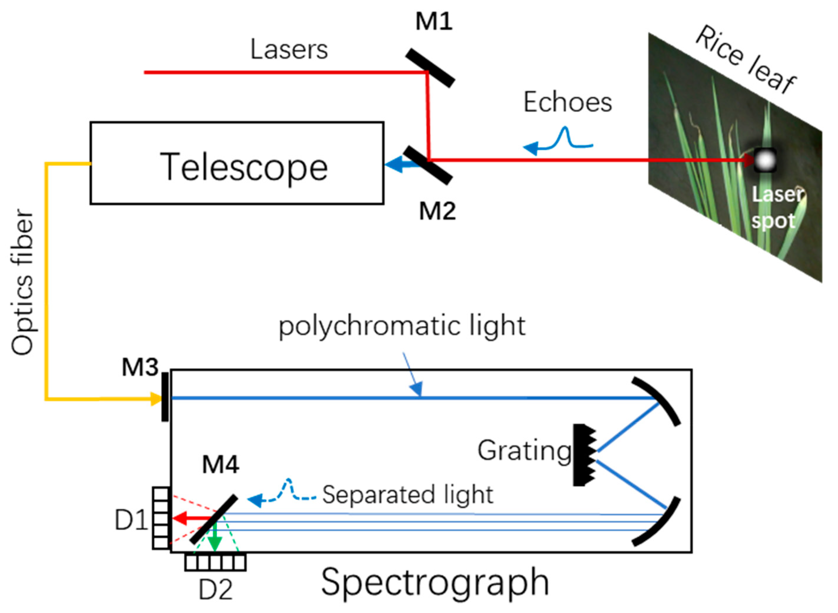
2.2. LiDAR Systems and Data Measurement

The HSL system used in this work consisted of some fundamental components, including laser emission, photovoltaic receiving and conversion and the data processing section (Figure 1). The light emission section of the HSL mainly contained a supercontinuum laser source (SuperK EXTREME, NKT Photonics Inc., DEN), which can generate a wide-band laser with a frequency of 20-40 kHz, an average output power of 100 mW, a broadband spectrum white light of ~450–2400 nm and a pulse duration of 1–2 ns [47,48]. The data collected by HSL represented the characteristic spectrum of the target in a range of 538–910 nm with the spectral resolution of 12 nm based on the APD array, which consisted of 32 separated channels with a spectral sensitive range of 300–920 nm (D1 in Figure 1). The components of LIFL system were similar to those of HSL, and the only difference with HSL was that the LIFL system had the ultraviolet excitation light source (355 nm, 20 Hz, Surelite OPO PLUS, USA) and a spectrograph with ICCD camera (D2 in Figure 1, Princeton Instrument SP2500i, USA) as the section of laser emission, and photovoltaic receiving and conversion, respectively. The laser source for LIFL is an Nd: YAG which has an output power of 1.5 mJ and width per pulse of 5 ns. The spectrograph can be controlled along with the direct commands through its USB or RS-232 port, so as to scan and then obtain S_f characteristics with a wide-range (360–800 nm) and high spectral resolution (0.5 nm). In order to eliminate the effects of light reflected from the laser, we placed a 355 nm long-pass edge filter (M3 in Figure 1) between the spectrograph and the optics fiber during S_f collection. The filter was shunted to the other side during the measurement of S_r. These two LiDAR systems, which had the same optics design, were used in collecting and focusing light signals into an achromatic telescope (with a diameter of 200 mm, MEADE, USA), and then transmiting the light signals reflected from the target surface to two photo-sensitive receiver ports on a SP2500i spectrometer (D1 for S_r, red and D2 for S_f, blue in Figure 1) through an optics fiber for photovoltaic conversion. Further details about the systems can be found in the study of Du et al. [40] and Yang et al. [49].

With these two LiDAR systems, spectra of S_r and S_f were measured at three different positions off the rice leaf vein for one sample, and five replications were carried out at the same position. Then, the characteristic spectra for one leaf were represented with the average of 15 spectra obtained by the above process. The laser spots of HSL and LIFL resided onto the measured position perpendicularly and completely.

As shown in Figure 2, differences among rice LNC levels are easily distinguished on the basis of some feature positions on the S_r and S_f curves measured by HSL (Figure 2a) and LIFL (Figure 2b) systems respectively. After the collection of the spectra, LNC values were determined using the Kjeldahl method [50], and then weighted and expressed as milligrams per gram of leaf dry matter. The LNC values in 2014 ranged from 2.5 to 4 mg/g, with an average (Ave) of 3.34 mg/g and standard deviation (SD) of 0.27 mg/g. In 2015, the LNC ranging from 1.1 mg/g to 4.4 mg/g had an Ave value of 2.84 mg/g and SD value of 0.61 mg/g.

3. Methods

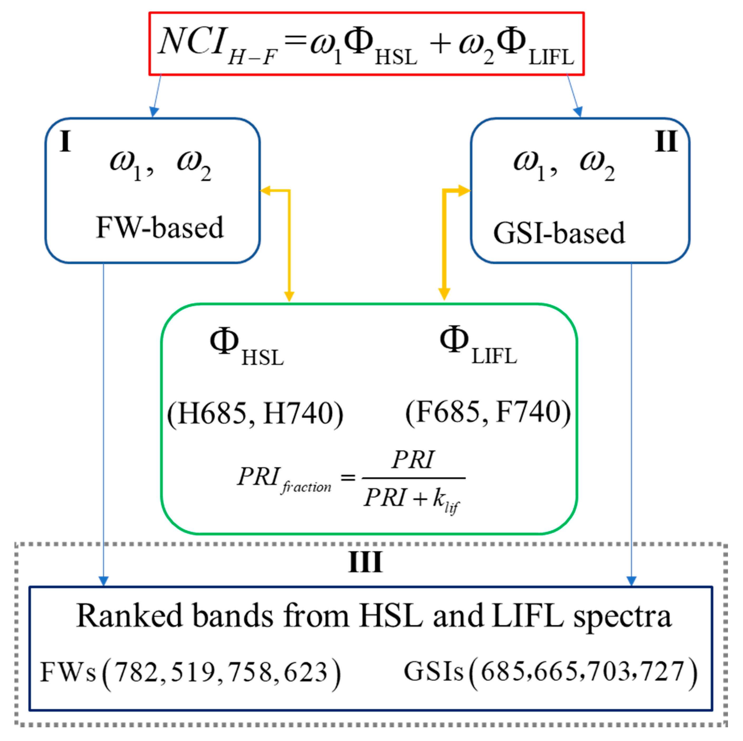
3.1. Overview of the Analysis Method

In this study, a SIs, called NCI_H-F, was constructed to estimate the rice LNC. This kind of SIs links the HSL and LIFL spectra to LNC through two factors (${\omega }_1$, ${\omega }_2$ in Equation (1)) which are closely related to the characteristic bands.

$$NC{I}_{H-F}={\omega }_1{\mathsf{\Phi }}_{\mathrm{HSL}}+{\omega }_2{\mathsf{\Phi }}_{\mathrm{LIFL}},$$

(1)

On the basis of two calculation methods for these factors, the analysis methods in this study were organized as shown in Figure 3: (I) FW-based NCI_H-F were utilized for estimation of rice LNC, and then (II) utilized based on GSIs. The results were respectively summarized in Section 4.1 and Section 4.2. (III) Finally, four characteristic bands from S_r and S_f data were respectively ranked and then selected based on the values of FW and GSI for the calculation of NCI_H-F, rather than designating them in 685, 740 nm. The estimation results were showed in Section 4.3. Meanwhile, a modified SI named PRI_fraction (Equations (7) and (8) in Section 4.1) [51] was proposed in steps (I) and (II) for the comparison experiment.

3.2. Two Methods for NCI_H-F Factor Calculation

The NCI_H-F values derived from HSL and LIFL data are linked in a linear form according to the contribution ratio of S_r (${\omega }_1$) and S_f (${\omega }_2$) to LNC, as determined with two methods described in Section 3.2.1 and Section 3.2.2. The values of ${\mathsf{\Phi }}_{\mathrm{HSL}}$ and ${\mathsf{\Phi }}_{\mathrm{LIFL}}$ in Equation (1) may represent the intensity of S_r and S_f in a single band (685 or 740 nm), and can represent the SIs derived from LiDAR data.

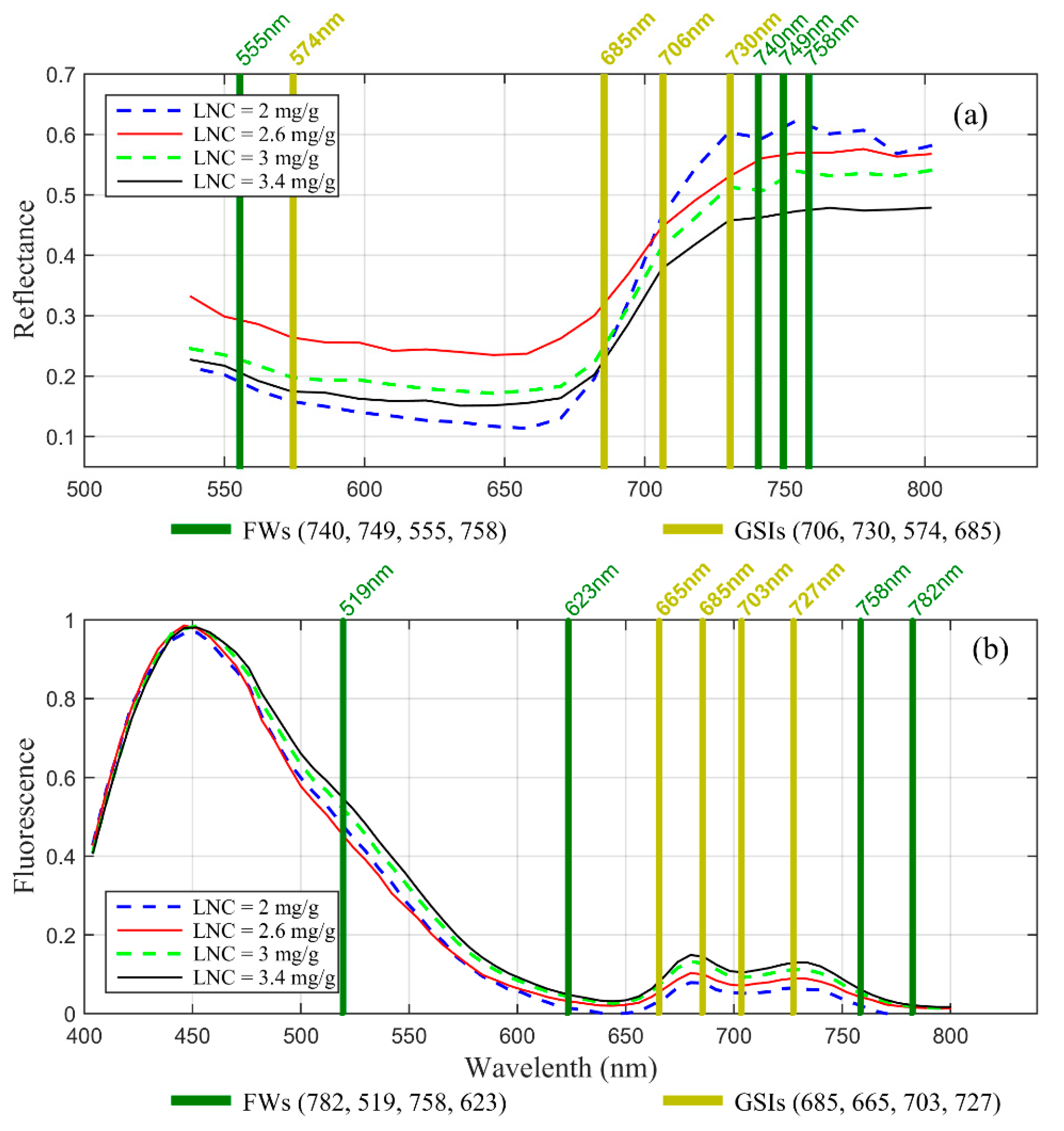
3.2.1. Feature Weights for Each Spectral Band

The FWs of each band represent the efficient indicators linking the spectra in wide-bands to biochemical contents. In this work, FWs were calculated on the basis of the divergence for each class divided according to vegetation species and biochemical contents. In the calculation process, a significant coefficient of band corresponding to class j, ${\eta }_j(\lambda )$ (j = 1, 2, …, m), was ranked in descending order with Equation (3) according to band sensitivity to the different biochemistry parameters. Subsequently, the FWs for each band were calculated using Equation (2), where $P_{\mathrm{re}-\mathrm{ranked}}^{\lambda }$ was the band position in the sequence of ${\eta }_j\left(\lambda \right)$ in Equation (3),

$$FWs\left(\lambda \right)=\frac{1}{n}{\displaystyle \sum _{j=1}^m\left(P_{\mathrm{re}-\mathrm{ranked}}^{\lambda }\right)}$$

(2)

$${\eta }_j\left(\lambda \right)=\frac{1}{n}\sum _{i=1}^n{\mu }_i{\left(E_{\lambda i}\right)}^2\left(i=1,2,\dots ,n\right)$$

(3)

where n is the number of bands, μ_i represents a divergence ratio of the ith band to all bands, and $E_{\lambda i}$ denotes the elements of eigenvectors of the covariance matrix for each class.

3.2.2. Global Sensitivity Indices for Each Spectral Band

In this section, the sensitivity indices of parameters to the changes in total spectra in each band were noted as the new weights for constructing NCI_H-F for LNC estimation. Given that k variables affect the variation characteristics of LNC in a spectrum, the set of parameter variables was defined as A = [$a_1$, $a_2$, …, $a_k$]. For A = [$a_1$], only one variable was present, and $a_i=\overline{a_i}$, the variance of $R(\lambda )$ was $\mathrm{Var}[R(\lambda \left)\right| \overline{a_i}]$. Generally, the value of $\overline{a_i}$ was unpredictable. Hence, the variance was unavailable. However, the expectation for $R(\lambda )$ can be calculated according to all the possible values of $a_i$, which can be substituted with the variance, noted as $\mathrm{E}[R(\lambda \left)\right| a_i]$. Then, the sensitivity of the single variable $GS{I}_i^s$ to the reflection spectrum can be characterized using the following formula:

$$GS{I}_i^s\left(\lambda \right)=\frac{Var(\mathrm{E}[R|a_i])}{Var(R)}.$$

(4)

This equation was used in a local sensitivity analysis called the first-order sensitivity index, which disregarded the influence of other parameters. In fact, a feature spectrum is not determined by a single variable but is the result of the interaction of many factors, and usually $GS{I}_{ij}^s(\lambda )\ge GS{I}_i^s(\lambda )+GS{I}_j^s(\lambda )$. In this work, a total sensitivity index (Equation (5)) with multivariable was calculated by taking the spatial autocorrelation coefficient $\gamma (\lambda )$ as the input condition, and was used as the basis for the priority ranking of sensitive bands.

$$GS{I}_k^s\left(\lambda \right)=\frac{Var(\mathrm{E}[R|\gamma (a_1,s_2,\dots ,a_k)])}{Var(R)}$$

(5)

Each variable shows unique sensitivity in different bands, and even the spectral intensity in the same band depends on multiple parameters. This attribute is not only a powerful basis for constructing NCI_H-F for LNC estimation, but also an essential analysis strategy for the inversion and extraction of specific biochemical parameters.

3.3. Artificial Neural Networks for LNC Estimation

In this section, an ANN with four training functions, namely, Levenberg–Marquardt Algorithm (trainlm), Bayesian regularization algorithm (trainbr), Quasi-Newton Algorithm (trainbfg), and one step secant algorithm (trainoss) were described, and then utilized for the prediction of rice LNC with the constructed NCI_H-F values.

The feed forward ANNs in this work consisted of three layers, namely input, hidden, and output, which were created, trained, and implemented in the Matlab 2014b environment. Four commonly used training functions were adopted respectively. Additionally, the ANN conditions were set as follows: minimum mean square error (MSE) of 10⁻³, minimum gradient of 10⁻⁶, and maximum iteration number (epochs) of 100. After the conditions were met, the ANNs iteration process was stopped. Other details about ANNs can be found in the work of Yegnanarayana [52] and the documents of software Matlab 2014b.

$$y=f_{non}\left({\displaystyle \sum _{i=1}^n{b}_i{X}_i+c_i}\right)$$

(6)

The nonlinear activation function f_non in Equation (6) was used in processing the iteration process. The function generated a y value as the predicted LNC, where b_i is the network weight and c_i is the bias, which were all adjusted along with the gradient-decreased MSE.

4. Results

Figure 2 shows the spectra of S_r and S_f collected by HSL and LIFL systems under four different LNC levels, and the distribution of prior LNC-sensitive bands on the S_r and S_f curves. The features of S_r and S_f in special bands were closely related to the LNC values of rice, which could be correctly measured by these two LiDAR systems, whether there was a positive or negative relationship. Thus, these two LiDAR systems were reliable remote sensing tools for rice feature spectra measurement, regardless of S_r or S_f characteristics under different LNC levels. Moreover, prior bands selected with FWs and GSIs were discretely distributed onto the S_r and S_f curves and covered most LNC-sensitive bands. This finding indicated that the analysis of feature weight and the global sensitivity of numerous factors to the spectral intensity in each special band was powerful potential method for selecting preferentially sensitive bands for vegetation biochemical estimation, especially N.

On the basis of a series of spectra of S_r and S_f collected by HSL and LIFL system, we constructed numerous combined SIs linked by FWs and GSIs for LNC estimation, and finally obtained some SIs with high R² (that >0.7 have been in bold in

Table 1. FW-based NCI_H-F used for LNC estimation and its corresponding R² and RMSE for the year of 2014 and 2015 respectively.

NCIH-F	2014-B		201402-H		2015-T		Spectral Variables
	R2	RMSE	R2	RMSE	R2	RMSE	${\mathbf{\Phi }}_{\mathbf{HSL}}$	${\mathbf{\Phi }}_{\mathbf{LIFL}}$
NCIH-F 0_W	0.74 c	0.28	0.70 c	0.45	*	*	$\sum (H685,H740)$	$\sum (F685,F740)$
NCIH-F 1_W	0.72 a	0.15	0.72 c	0.32	0.61 d	0.28	$\sum (H685,H740)$	$\sum (F685,F740)$
NCIH-F 2_W	0.51 b	0.18	0.62 c	0.30	0.79 c	0.23	H685	F685
PRIfraction_W	0.57 c	0.32	0.74 c	0.23	0.70 c	0.13	/	F740

Note: The training functions of ANN models include ^a trainlm, ^b trainbr, ^c trainbfg, and ^d trainoss, with the same marks in Table 2 and Table 4.

,

Table 2. GSI-based NCIH-F used for LNC estimation and its corresponding R² and RMSE for year of 2014 and 2015 respectively.

NCIH-F	2014-B		201402-H		2015-T		Spectral Variables
	R2	RMSE	R2	RMSE	R2	RMSE	${\mathbf{\Phi }}_{\mathbf{HSL}}$	${\mathbf{\Phi }}_{\mathbf{LIFL}}$
NCIH-F 1_S	0.76 c	0.31	0.82 d	0.27	0.70 c	0.2	$\sum (H685,H740)$	$\sum (F685,F740)$
NCIH-F 2_S	0.75 c/0.71 d	0.18/0.29	0.63 d	0.35	0.45 c	0.36	H740	F740
PRIfraction_S	0.58 a	0.35	0.67 d	0.26	0.74 b	0.16	/	F740

, and Table 4) for LNC prediction models. Generally, the combined SIs performed well in rice LNC modeling in the specified bands, i.e., 685 and 740 nm. Subsequently, we analyzed the ability of NCI_H-F in four prior bands on LNC estimation (Section 4.3), and these ranked bands were selected according to FW and GSI values respectively.

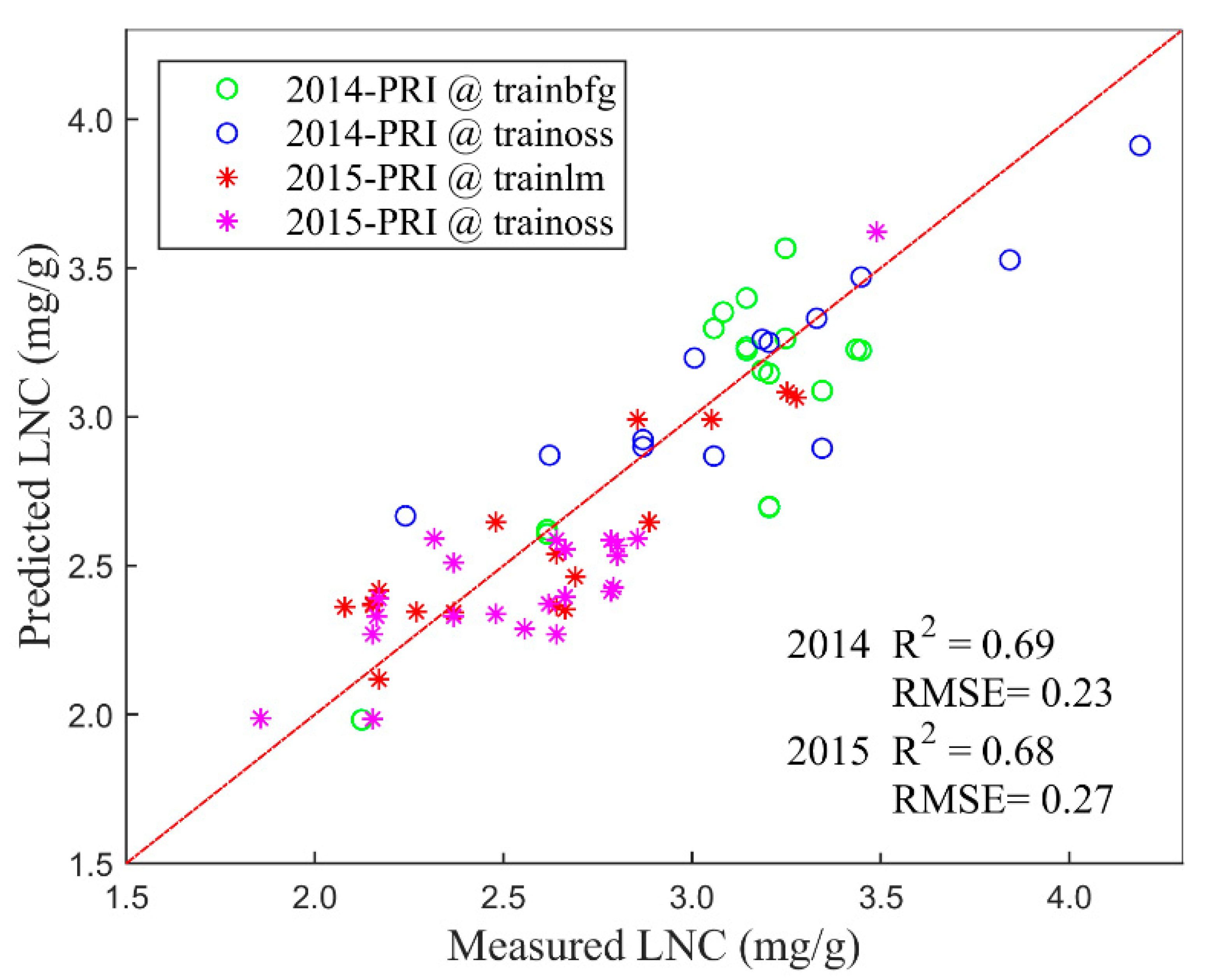
4.1. LNC Estimation Using FW-Based NCI_H-F

On the basis of the construction form of NCI_H-F in Equation (1), four FW-based NCI_H-F with high R² values were obtained during rice LNC estimation (Table 1). The superscripts (a, b, c and d) of each R² in Table 1 indicates the four training functions of ANN models used in examining the relationship between LNC and NCI_H-F. The obtained NCI_H-F can be classified into two types, namely, the sum of HSL and LIFL variables in two specified bands (685 and 740 nm, marked with NCI_H-F*_W in Table 1), that is, there are four variables (H685, H740, F685 and F740). Another type is the modified photochemical reflectance index (PRI), called PRI_fraction (Equation (7)) which is also presented in Table 1. Similar to the combined form of NCI_H-F, the bands used in PRI_fraction, including 531, 570 and 740 nm, were also replaced with FWs*$\mathsf{\Phi }$, or GSIs*$\mathsf{\Phi }$ in the subsequent analysis. PRI is commonly used as an indicator of vegetation photosynthesis process. In this study, the item k_lif in Equation (7) was replaced with F740, which is expressed Equation (9) as follows:

$${PRI}_{fraction}=\frac{PRI}{PRI+k_{lif}}$$

(7)

$$PRI=\frac{I_{531}-I_{570}}{I_{531}+I_{570}}$$

(8)

$${PRI}_{fraction}=\frac{PRI}{PRI+F_{740}}$$

(9)

For NCI_H-F 0_W in Table 1, we set a constant weight of 0.5, whereas ${\omega }_1$ = ${\omega }_2$ = 0.5 for each spectral variable, and obtained an R² of 0.74 in the booting stage and a R² of 0.7 in the heading stage of 2014. Replacing ω₁ and ω₂ with the corresponding FWs for 685 and 740 nm alternatively (NCI_H-F 1_W), the model results were improved by more than 0.8 and 0.72 in 2014 respectively. In 2015, the NCI_H-F with a constant contribution weight of 0.5, had no outstanding performance in LNC estimation. By replacing the constant weights with their FWs, we could obtain an R² of 0.61 for NCI_H-F 1_W. For NCI_H-F 2_W, the spectral variables of NCI_H-F were single band (H685, F685), which were different from those of NCI_H-F 1_W. Table 1 shows that the R² of NCI_H-F 1_W model can be more than 0.79 for 2015, while is less than 0.7 for both stages of 2014.

4.2. LNC Estimation Using GSI-Based NCI_H-F

As shown in Section 4.1, the same kinds of NCI_H-F obtained R² values of >0.7 in this section. The difference with FW-based NCI_H-F was that the spectral variables are connected with GSIs, and some items used to construct NCI_H-F in the same form had changed. For example, for NCI_H-F 2_S the spectral variable was (H740, F740), and not the (H685, F685) in NCI_H-F 2_W. The NCI_H-F 2_S model for LNC estimation performed well in 2014-B, but obtained an unsatisfactory result in 2014-H, and even a bad performance in 2015-T. When the GSI-based NCI_H-F in four spectral variables was used, the NCI_H-F 1_S was available in 2014 and 2015 data, obtaining a mean R² of 0.76 (Table 2). However, for PRI_fraction_S, the ANN model performed well with R² of 0.74 for the 2015-T data. The difference in performance can be found in Section 4.1, which shows a relatively good results in 2014-H and 2015-T. Thus, the spectra in different years can be a noteworthy issue in the LNC estimation of rice.

The PRI has been demonstrated to be a robust spectral index that is closely related to the vegetation photosynthesis process in leaf and canopy scales [2]. PRI has the same construction form as NDVI, which is calculated in 531 and 570 nm (Equation (8)). As well, PRI had been proved the available ability on LNC estimation with different training functions of ANNs in this study. In comparison with PRI, we found that the PRI_fraction with FW- and GSI-based weights could be a more effective index for LNC estimation in rice. For example, the total mean R² of PRI was 0.68 for the 2015 data (Figure 4); this value was slightly lower than the PRI_fraction values represented in Table 1 and Table 2. Thus, the FW- and GSI-based weights could be efficiently used in improving the performance of PRI in LNC estimation on the basis of S_r-S_f features obtained with HSL and LIFL systems. Notably, the mean R² of PRI was 0.69 in both stages of 2014, and these values were higher than the PRI_fraction modified based on the FWs and GSIs in Table 1 and Table 2. These results indicated that the growth stages and years of rice served as relatively sensitive factor which affected the model performance of combined SIs in LNC estimation.

4.3. NCI_H-F in Ranked Bands for LNC Estimation

In this section, the bands used to construct NCI_H-F were selected preferentially based on the FW and GSI values. Then, the first four prior bands were selected as the spectral variables for the calculation of NCI_H-F, and modeling of rice LNC with the ANN method. These prior bands are the LNC-sensitive characteristics to rice LNC, and they are discretely distributed onto some critical positions of HSL and LIFL spectra (Figure 2). Concretely, the positive relationship between N level and S_r intensity can be changed to a negative relationship in approximately 700 nm. Alternatively, for S_f, the double-peak spectra in 650–750 nm regularly increased along with the N level.

Based on the positions of these selected bands, four FW-based prior variables for S_r were almost distributed in the near-infrared band. These variables were significantly important to the GSV because of the reflectance and absorption characteristics of pigments in vegetation leaf. In S_f curve, FW-based prior bands were distributed discretely over the whole interest range of 450–800 nm (Figure 2b). For the prior bands selected by GSI values, two bands located in the “red-edge” position of S_r curve, while all of them located in the bands centered about the double-peak characteristics in S_f curve.

With these selected bands, NCI_H-F was calculated and then unitized in estimating LNC for the 2014- and 2015-year data based on ANNs method. The results could be found in Figure 5, which showed the optimal R² among these band-ranked NCI_H-F. In comparison with the use of specified bands in the above section, the NCI_H-F with ranked bands generally had an acceptable modeling accuracy for the 2014 and 2015 data, whereas for GSI-based NCI_H-F the R² was less than 0.7 (Figure 5b).

Linking factors (ω₁ and ω₂) for NCI_H-F in Equation (1) were listed in

Table 3. Values of ${\omega }_1$ and ${\omega }_2$ in Equation (1) calculated with FWs and GSIs for four spectral variables, namely (H685 H740) and (F685 F740).

NCIH-F		${\mathbf{\Phi }}_{\mathbf{HSL}}$	${\mathit{\omega }}_1$	${\mathbf{\Phi }}_{\mathbf{LIFL}}$	${\mathit{\omega }}_2$
FW-based	NCIH-F 0_W	$\sum (F685,F740)$	0.50	$\sum (F685,F740)$	0.50
	NCIH-F 1_W	$\sum (F685,F740)$	0.52	$\sum (F685,F740)$	0.48
	NCIH-F 2_W	H685	0.27	F685	0.73
	PRIfraction_W	&	/	F740	0.35
GSI-based	NCIH-F 1_S	$\sum (F685,F740)$	0.52	$\sum (F685,F740)$	0.48
	NCIH-F 2_S	H740	0.50	F740	0.50
	PRIfraction_S	&	/	F740	0.24

Note: & The ${\mathsf{\Phi }}_{\mathrm{HSL}}$ variable for PRI_fraction is related with the Sr features in band of 531 and 570 nm, and the values of ${\omega }_2$ are respectively calculated with the FWs and GSIs in bands of 531 and 570 nm following Equations (7) and (8).

, in which the sum variables (H685 H740) and (F685 F740) for NCI_H-F 1_W and _S had the comparative contribution to NCI_H-F (approximately 0.5). However, for FW-based NCI_H-F, the values of ω₁ and ω₂ for single variable, such as H685 and F685, were 0.27 and 0.73 respectively, indicating that the S_r features from HSL data had a weaker contribution to LNC than that using S_f from the LIFL data. For GSI-based NCI_H-F, namely NCI_H-F 2_S with variables of H740 and F740, had the near factor values (ω₁ = 0.50 and ω₂ = 0.50). For the PRI_fraction, the variable in the denominator was replaced by F740, with FW and GSI values as the contribution ratios ω₁ and ω₁, and being less than 0.4 (0.35 and 0.24 respectively).

5. Discussion

5.1. Comparison with Previously Published Methods

Both S_r and S_f features are the important indicators for GSV monitoring. Thus, we attempted to find an effective way to combine these two spectral properties together for LNC modeling. The first thing we could conceive was to construct a common SI based on the HSL and LIFL data, which is sensitive to rice LNC. Vegetation LNC is thought to be codetermined by S_r-S_f characteristics, and the values of ${\omega }_1$ and ${\omega }_2$ can be considered as their corresponding contribution ratios to LNC. Some combined indices derived from HSL and LIFL data had been proposed in some previous works. Shi et al. [40] developed a kind of combined index with the similar form as NDVI by combining HSL and LIFL spectral variables, called N(H685, F685) and N(H740, F740) in Equation (10). However, these combined indices performed poorly, and even had a weaker ability for LNC modeling than the ratio indices obtained by using HSL or LIFL spectra separately. In this work, we linked the HSL and LIFL variables to rice LNC as expressed in a form of Equation (1), and named as NCI_H-F, which was constructed by significant factor, such as FWs and GSIs for each band. Accordingly, we improved the estimation results efficiently. In addition, we found that adding more characteristics entered as the model input did not necessarily improve the results. Conversely, the combined SIs with only two spectral variables showed the same good model R², such as the NCI_H-F 2_S in Table 2, and HL-NormIndex_W and _S in

Table 4. Comparison of estimated LNC results between the published combined indices in Du et al. and the FW/GSI-based NCI_H-F in the same form as NDVI based on the data from 2014- and 2015-year. (SI of N(H685, F685) and N(H740, F740) can be calculated with Equations (10) and (11), respectively).

Combined Index	2014-B		201402-H		2015-T
	R2	RMSE	R2	RMSE	R2	RMSE
N(H685, F685)	0.408	0.479	0.698	0.269	0.479	0.499
N(H740, F740)	0.488	0.579	0.597	0.358	0.498	0.491
HL-NormIndex_W	0.74 a/0.71 d	0.11/0.16	0.81 b	0.15	0.72 c	0.14
HL-NormIndex_S	0.73 c	0.22	0.70 d	0.23	0.82 c	0.16

. Hence, multiplying the bands with their corresponding FWs or GSIs may efficiently combine S_r and S_f together for LNC estimation, and the ability of SIs for LNC estimation relies mostly on the combination forms of spectral variables.

$$N\left(H\mathit{685},F\mathit{585}\right)=\frac{H\mathit{685}-F\mathit{685}}{H\mathit{685}+F\mathit{685}}$$

(10)

$$N\left(H\mathit{740},F\mathit{740}\right)=\frac{H\mathit{740}-F\mathit{740}}{H\mathit{740}+F\mathit{740}}$$

(11)

Moreover, with the purpose of supporting the above conclusion and further improving the SIs performance on LNC estimation [38], we replaced the spectral variables in Equation (9), including H685, F685, H740 and F740, by FWs and GSIs multiplied with the corresponding bands, and then conducted LNC modeling with these modified SIs. Table 4 showed that the model performance was improved, and some R² values distinctly reached 0.82 (HL-NormIndex_W and _S) while with a lower RMSE. Thus, the FW- and GSI-based methods in this work may be used to efficiently construct combined SIs for LNC estimation and improve the model performance significantly.

5.2. Prior Bands Selection

In Figure 5, the FW-based combined SIs performed better in linking NCI_H-F to rice LNC than that SIs using GSI values. The selected bands from the HSL and LIFL spectrum in Figure 2 can also explain this result. The prior bands ranked based on FWs were regularly located in the major S_r range, thereby covering more features related to LNC, such as the “red-edge” position, and Chl absorption area. Comparatively, the GSI-based NCI_H-F in this work was usually calculated with the bands in the red-range but lacked some characteristics, which might decrease its universality in estimating LNC or other biochemicals. Meanwhile, the prior bands selected with mathematics (FWs) or physical model (GSIs) cannot consider all these variables from different experimental and environmental situations. However, the spectral variables in 685 and 740 nm are the important features for GSV, which has been determined by many researchers [53]. Thus, the results of NCI_H-F in specified bands obtaining a better model performance for LNC estimation than that in four prior bands can be reasonable.

The spectra collected with optical sensors, even for the active LiDAR used in this work, are the direct indicators for Chl contents in vegetation leaf, and these indicators can be used as the basis of LNC monitoring by remote sensing method. However, the LNC and Chl of vegetation are not same parameters after all, even though they are closely related to each other. In this work, FWs for each band were calculated based on a mass of modeled and collected spectra [54,55] and LNC measurement in the laboratory, whereas the GSIs were analyzed based on the fluorescence model with inputs that do not contain LNC [56]. This may contribute to the prior bands being selected with GSIs are not Chl-sensitive for LNC. Thus, GSI-based bands do not cover the total characteristics for LNC in HSL and LIFL spectra in Figure 2, indicating that the GSI-based NCI_H-F obtained a lower R² than that using FWs.

5.3. Limitation and Future Research

In this study, rice LNC was successfully estimated by NCI_H-F. However, the model should be recalibrated when applied to other vegetations or even to rice grown under different environmental conditions. Moreover, the ANN model used in this study greatly depended on the selection of training and validation dataset, which would change during LNC modeling. Thus, a universal and dataset-independent method should be determined for the combination of the spectra of S_r and S_f for LNC or other biochemical estimation. This study attempted to solve this problem by forming a novel SI which linked S_r and S_f in a linear equation with two factors, namely, FWs and GSIs. However, we should admit that the FW- and GSI-based NCI_H-F was conducted based on the spectra from two separate datasets, which might contribute errors to the ANN models of LNC estimation because of the non-uniform dataset.

Furthermore, the FW and GSI values of each band represented quite a contribution ratio of S_r and S_f to the LNC, although a certain physical significance was observed in the linear form NCI_H-F to some extent. The two factors were calculated using a statistical method, especially for FWs, which greatly depended on sample spectra. In a recent study, the biochemical estimation of vegetation was conducted based on the radiative transfer models (RTMs), including the SCOPE model (Soil Canopy Observation, Photochemistry and Energy fluxes) proposed by Christiaan et al. [57,58] and one of the separated components of SCOPE, namely, the Fluspect-B model [59]. Unlike the PROSPECT model with leaf reflectance and transmittance spectra [55] and the FluorMODleaf model with leaf S_f [60], both SCOPE and Fluspect-B can simulate the total spectra of S_r and S_f simultaneously, rather than being univocal for generating a special spectrum without considering all feature spectra together to estimate the vegetation biochemicals [61]. Based on the uniform spectra of S_r and S_f generated by SCOPE or Fluspect-B model, the FWs and GSIs for each band can be calculated, which might further improve the performance and universality of the ANN model in rice LNC estimation, and even for some other biochemicals, such as moisture, dry matter, and so on, which are important indicators for the GSV, as well as for land coverage and change detection, which are critically significant for the analysis of the carbon–nitrogen cycle [62], near surface atmosphere temperature [63,64,65], and dynamics variation in permafrost region [66,67] among other fields.

6. Conclusions

This study proposed a combined spectral index, namely, the NCI_H-F for LNC estimation. The NCI_H-F was constructed in a linear combination form linked spectra of S_r and S_f collected with HSL and LIFL systems to rice LNC based on two factors, namely FWs and GSIs for each feature band. By using an additive SI in two specific bands (685 and 740 nm), the NCI_H-F values in this work could be utilized to estimate rice LNC accurately under multi-year rice samples. Thus, the NCI_H-F is the available and reliable combined form for combining HSL and LIFL spectral characteristics for rice LNC estimation. Simultaneously, the modified PRI, called PRI_fraction, demonstrated a satisfactory performance in rice LNC estimation by replacing some items with S_f variables, multiplying corresponding FWs and GSIs in 740 nm. These results showed that FWs and GSIs could indicate the main contribution of each band to LNC, which were essential and valuable parameters for constructing novel SIs for LNC estimation of rice. Moreover, the FW and GSI values for each feature band were multiplied to some previous combined SIs, for instance, N(H685, F685) and N(H740, F740), and improved the model performance of LNC estimation significantly. This result further supported the above conclusion that FW- and GSI-based NCI_H-F is efficient in remotely sensing rice LNC, and combining S_r and S_f features in a linear form is a reliable way to improve the model performance in LNC estimation based on the HSL and LIFL spectra.

References

1. Clevers, J.G.; Gitelson, A.A. Remote estimation of crop and grass chlorophyll and nitrogen content using red-edge bands on Sentinel-2 and -3. Int. J. Appl. Earth Obs. Geoinf. 2013, 23, 344–351. [Google Scholar] [CrossRef]
2. Kergoat, L.; Lafont, S.; Arneth, A.; Le Dantec, V.; Saugier, B. Nitrogen controls plant canopy light-use efficiency in temperate and boreal ecosystems. J. Geophys. Res. Biogeosci. 2008, 113, 1–19. [Google Scholar] [CrossRef] [Green Version]
3. Ikawa, H.; Chen, C.P.; Sikma, M.; Yoshimoto, M.; Sakai, H.; Tokida, T.; Usui, Y.; Nakamura, H.; Ono, K.; Maruyama, A.; et al. Increasing canopy photosynthesis in rice can be achieved without a large increase in water use-A model based on free-air CO2 enrichment. Glob. Chang. Biol. 2018, 24, 1321–1341. [Google Scholar] [CrossRef] [PubMed]
4. Dechant, B.; Cuntz, M.; Vohland, M.; Schulz, E.; Doktor, D. Estimation of photosynthesis traits from leaf reflectance spectra: Correlation to nitrogen content as the dominant mechanism. Remote Sens. Environ. 2017, 196, 279–292. [Google Scholar] [CrossRef]
5. Diacono, M.; Rubino, P.; Montemurro, F. Precision nitrogen management of wheat. A review. Agron. Sustain. Dev. 2012, 33, 219–241. [Google Scholar] [CrossRef]
6. Zhang, N.; Wang, M.; Wang, N. Precision agriculture—A worldwide overview. Comput. Electr. Agric. 2002, 36, 113–132. [Google Scholar] [CrossRef]
7. Schlemmer, M.; Gitelson, A.; Schepers, J.; Ferguson, R.; Peng, Y.; Shanahan, J.; Rundquist, D. Remote estimation of nitrogen and chlorophyll contents in maize at leaf and canopy levels. Int. J. Appl. Earth Obs. Geoinf. 2013, 25, 47–54. [Google Scholar] [CrossRef] [Green Version]
8. Delegido, J.; Pasqualotto, N.; van Wittenberghe, S.; Verrelst, J.; Rivera, J.P.; Moreno, J. Retrieval of canopy water content of different crop types with two new hyperspectral indices: Water Absorption Area Index and Depth Water Index. Int. J. Appl. Earth Obs. Geoinf. 2018, 67, 69–78. [Google Scholar]
9. Wang, C.; Nie, S.; Xi, X.; Luo, S.; Sun, X. Estimating the biomass of maize with hyperspectral and LiDAR data. Remote Sens. 2016, 9, 11. [Google Scholar] [CrossRef] [Green Version]
10. Yi, Q.X.; Huang, J.F.; Wang, F.M.; Wang, X.Z.; Zhan, Y. Monitoring rice nitrogen status using hyperspectral reflectance and artificial neural network. Environ. Sci. Tech. 2007, 41, 6770–6775. [Google Scholar] [CrossRef]
11. Knyazikhin, Y.; Schull, M.A.; Stenberg, P.; Mõttus, M.; Rautiainen, M.; Yang, Y.; Marshak, A.; Carmona, P.L.; Kaufmann, R.K.; Lewis, P.; et al. Hyperspectral remote sensing of foliar nitrogen content. Proc. Natl. Acad. Sci. USA 2013, 110, E185–E192. [Google Scholar] [CrossRef] [PubMed] [Green Version]
12. Jones, H.G.; Vaughan, R.A. Remote Sensing of Vegetation: Principles, Techniques, and Applications; Oxford University Press: Oxford, UK, 2010; p. 134. [Google Scholar]
13. Li, F.; Mistele, B.; Hu, Y.; Chen, X.; Schmidhalter, U. Reflectance estimation of canopy nitrogen content in winter wheat using optimised hyperspectral spectral indices and partial least squares regression. Eur. J. Agron. 2014, 52, 198–209. [Google Scholar] [CrossRef]
14. Johnson, L.F. Nitrogen influence on fresh-leaf NIR spectra. Remote Sens. Environ. 2001, 78, 314–320. [Google Scholar] [CrossRef]
15. Curran, P.J.; Dungan, J.L.; Peterson, D.L. Estimating the foliar biochemical concentration of leaves with reflectance spectrometry: Testing the Kokaly and Clark methodologies. Remote Sens. Environ. 2001, 76, 349–359. [Google Scholar] [CrossRef]
16. Portz, G.; Molin, J.; Jasper, J. Active crop sensor to detect variability of nitrogen supply and biomass on sugarcane fields. Precis. Agric. 2012, 13, 33–44. [Google Scholar] [CrossRef]
17. Gong, P.; Pu, R.; Heald, R. Analysis of in situ hyperspectral data for nutrient estimation of giant sequoia. Int. J. Remote Sens. 2002, 23, 1827–1850. [Google Scholar] [CrossRef]
18. Li, F.; Miao, Y.; Hennig, S.D.; Gnyp, M.L.; Chen, X.; Jia, L.; Bareth, G. Eevaluating hyperspectral vegetation indices for estimating nitrogen concentration of winter wheat at different growth stages. Precis. Agric. 2010, 11, 335–357. [Google Scholar] [CrossRef]
19. Pengfei, C.; Jihua, W.; Wenjiang, H.; Baoguo, L. Research of new vegetation index for estimating crop canopy biomass. Spectrosc. Spectr. Anal. 2010, 2, 512–517. [Google Scholar]
20. Tian, Y.C.; Gu, K.J.; Chu, X.; Yao, X.; Cao, W.X.; Zhu, Y. Comparison of different hyperspectral vegetation indices for canopy leaf nitrogen concentration estimation in rice. Plant Soil 2014, 376, 193–209. [Google Scholar] [CrossRef]
21. Du, L.; Wei, G.; Shuo, S.; Jian, Y.; Jia, S.; Bo, Z.; Shalei, S. Estimation of rice leaf nitrogen contents based on hyperspectral LIDAR. Int. J. Appl. Earth Obs. Geoinf. 2016, 44, 136–143. [Google Scholar] [CrossRef]
22. Liu, L.; Guan, L.; Liu, X. Directly estimating diurnal changes in GPP for C3 and C4 crops using far-red sun-induced chlorophyll fluorescence. Agric. For. Meteorol. 2017, 232, 1–9. [Google Scholar] [CrossRef]
23. Grace, J.; Nichol, C.; Disney, M.; Lewis, P.; Quaife, T.; Bowyer, P. Can we measure terrestrial photosynthesis from space directly, using spectral reflectance and fluorescence? Glob. Chang. Biol. 2010, 13, 1484–1497. [Google Scholar] [CrossRef]
24. Živčák, M.; Olšovská, K.; Slamka, P.; Galambošová, J.; Rataj, V.; Shao, H.; Brestič, M. Application of chlorophyll fluorescence performance indices to assess the wheat photosynthetic functions influenced by nitrogen deficiency. Plant Soil Environ. 2014, 60, 210–215. [Google Scholar] [CrossRef] [Green Version]
25. Apostol, S.; Viau, A.A.; Tremblay, N. A comparison of multiwavelength laser-induced fluorescence parameters for the remote sensing of nitrogen stress in field-cultivated corn. Can. J. Remote Sens. 2007, 33, 150–161. [Google Scholar] [CrossRef]
26. Janušauskaite, D.; Feiziene, D. Chlorophyll fluorescence characteristics throughout spring triticale development stages as affected by fertilization. Acta Agric. Scand. Sect. B-Soil Plant Sci. 2012, 62, 7–15. [Google Scholar]
27. Günther, K.; Dahn, H.-G.; Lüdeker, W. Remote sensing vegetation status by laser-induced fluorescence. Remote Sens. Environ. 1994, 47, 10–17. [Google Scholar] [CrossRef]
28. Subhash, N.; Mohanan, C. Laser-induced red chlorophyll fluorescence signatures as nutrient stress indicator in rice plants. Remote Sens. Environ. 1994, 47, 45–50. [Google Scholar] [CrossRef]
29. Sun, Y.; Guo, P.; Zhao, J.; Yu, Z. Effect of nitrogen application rate on flag leaf chlorophyll fluorescence characteristics and yield in wheat under integration of water and fertilizer. J. Triticeae Crop. 2018, 38, 988–994. [Google Scholar]
30. Yang, Y.; Wang, X.; Li, C.; Zhao, B.; Bai, R. Detection of pepper leaves nitrogen contents in greenhouse based on chlorophyll fluorescence image. J. Hunan Agric. Univ. (Nat. Sci.) 2017, 43, 108–111. [Google Scholar]
31. Yang, J.; Shi, S.; Gong, W.; Du, L.; Ma, Y.Y.; Zhu, B.; Song, S.L. Application of fluorescence spectrum to precisely inverse paddy rice nitrogen content. Plant Soil Environ. 2015, 61, 182–188. [Google Scholar] [CrossRef] [Green Version]
32. Jasper, J.; Reusch, S.; Link, A. Active sensing of the N status of wheat using optimized wavelength combination: Impact of seed rate, variety and growth stage, in Precision Agriculture’09: Papers. In Proceedings of the the 7th European Conference on Precision Agriculture, Wageningen, The Netherlands, 6–8 July 2009; Volume 2009, p. 923. [Google Scholar]
33. Chen, P.; Haboudane, D.; Tremblay, N.; Wang, J.; Vigneault, P.; Li, B. New spectral indicator assessing the efficiency of crop nitrogen treatment in corn and wheat. Remote Sens. Environ. 2010, 114, 1987–1997. [Google Scholar] [CrossRef]
34. Chappelle, E.W.; Wood, F.M.; McMurtrey, J.E.; Newcomb, W.W. Laser-induced fluorescence of green plants. 1: A technique for the remote detection of plant stress and species differentiation. Appl. Opt. 1984, 23, 134–138. [Google Scholar] [CrossRef] [PubMed]
35. Zarco-Tejada, P.J.; Miller, J.R.; Mohammed, G.H.; Noland, T.L. Chlorophyll fluorescence effects on vegetation apparent reflectance: I. Leaf-level measurements and model simulation. Remote Sens. Environ. 2000, 74, 582–595. [Google Scholar] [CrossRef]
36. Zarco-Tejada, P.J.; Miller, J.R.; Mohammed, G.H.; Noland, T.L.; Sampson, P.H. Chlorophyll fluorescence effects on vegetation apparent reflectance: II. Laboratory and airborne canopy-level measurements with hyperspectral data. Remote Sens. Environ. 2000, 74, 596–608. [Google Scholar] [CrossRef]
37. Du, S.S.L.; Jian, Y.; Jia, S.; Wei, G. Using different regression methods to estimate leaf nitrogen content in rice by fusing hyperspectral LiDAR data and laser-induced chlorophyll fluorescence data. Remote Sens. 2016, 8, 526. [Google Scholar] [CrossRef] [Green Version]
38. Jian, Y.; Du, L.; Jia, S.; Zhengbing, Z.; Biwu, C.; Shi, S.; Wei, G.; Shalei, S. Estimating the leaf nitrogen content of paddy rice by using the combined reflectance and laser-induced fluorescence spectra. Opt. Express 2016, 24, 19354–19365. [Google Scholar]
39. Weersink, R.; Patterson, M.S.; Diamond, K.; Silver, S.; Padgett, N. Noninvasive measurement of fluorophore concentration in turbid media with a simple fluorescence/reflectance ratio technique. Appl. Opt. 2001, 40, 6389–6395. [Google Scholar] [CrossRef]
40. Du, S.S.L.; Jian, Y.; Wei, W.; Jia, S.; Biwu, C.; Wei, G. Potential of spectral ratio indices derived from hyperspectral LiDAR and laser-induced chlorophyll fluorescence spectra on estimating rice leaf nitrogen contents. Opt. Express 2017, 25, 6539–6549. [Google Scholar] [CrossRef]
41. Huang, R.; He, M. Band selection based on feature weighting for classification of hyperspectral data. IEEE Geosci. Remote Sens. Lett. 2005, 2, 156–159. [Google Scholar] [CrossRef]
42. Kavzoglu, T.; Mather, P.M. The role of feature selection in artificial neural network applications. Int. J. Remote Sens. 2002, 23, 2919–2937. [Google Scholar] [CrossRef]
43. Serpico, S.B.; Bruzzone, L. A new search algorithm for feature selection in hyperspectral remote sensing images. IEEE Trans. Geosci. Remote Sens. 2001, 39, 1360–1367. [Google Scholar] [CrossRef]
44. Cannavó, F. Sensitivity analysis for volcanic source modeling quality assessment and model selection. Comput. Geosci. 2012, 44, 52–59. [Google Scholar] [CrossRef]
45. Li, P.; Wang, Q. Retrieval of leaf biochemical parameters using PROSPECT inversion: A new approach for alleviating ill-posed problems. IEEE Trans. Geosci. Remote Sens. 2011, 49, 2499–2506. [Google Scholar]
46. Stocker, T.; Qin, D.; Plattner, G.; Tignor, M.; Allen, S.; Boschung, J.; Nauels, A.; Xia, Y.; Bex, B.; Midgley, B. IPCC, 2013: Climate change 2013: The physical science basis. In Contribution of Working Group I to the Fifth Assessment Report of the Intergovernmental Panel on Climate Change; IPCC: Geneva, Switzerland, 2013. [Google Scholar]
47. Ceolato, R.; Riviere, N.; Hespel, L. Reflectances from a supercontinuum laser-based instrument: Hyperspectral, polarimetric and angular measurements. Opt. Express 2012, 20, 29413–29425. [Google Scholar] [CrossRef]
48. Nevalainen, O.; Hakala, T.; Suomalainen, J.; Mäkipää, R.; Mikko, P.; Anssi, K.; Sanna, K. Fast and nondestructive method for leaf level chlorophyll estimation using hyperspectral LiDAR. Agric. For. Meteorol. 2014, 198, 250–258. [Google Scholar] [CrossRef]
49. Jian, Y.; Wei, G.; Shi, S.; Du, L.; Sun, J.; Zhu, B.; Yingying, M.; Shalei, S. Vegetation identification based on characteristics of fluorescence spectral spatial distribution. RSC Adv. 2015, 5, 56932–56935. [Google Scholar]
50. Wutzke, K.; Heine, W. A century of Kjeldahl’s nitrogen determination. Z. Fur Med. Lab. 1984, 26, 383–388. [Google Scholar]
51. Paul-Limoges, E.; Damm, A.; Hueni, A.; Liebisch, F.; Eugster, W.; Schaepman, M.E.; Buchmann, N. Effect of environmental conditions on sun-induced fluorescence in a mixed forest and a cropland. Remote Sens. Environ. 2018, 219, 310–323. [Google Scholar]
52. Yegnanarayana, B. Artificial Neural Networks; PHI Learning Pvt. Ltd.: Delhi, India, 2009. [Google Scholar]
53. Lichtenthaler, H.K.; Rinderle, U. The role of chlorophyll fluorescence in the detection of stress conditions in plants. Crit. Rev. Anal. Chem. 1988, 19, S29–S85. [Google Scholar] [CrossRef]
54. Wang, Z.; Skidmore, A.K.; Wang, T.; Darvishzadeh, R.; Hearne, J. Applicability of the PROSPECT model for estimating protein and cellulose + lignin in fresh leaves. Remote Sens. Environ. 2015, 168, 205–218. [Google Scholar] [CrossRef]
55. Jacquemoud, S.; Baret, F. PROSPECT: A model of leaf optical properties spectra. Remote Sens. Environ. 1990, 34, 75–91. [Google Scholar] [CrossRef]
56. Zarco-Tejada, P.J.; Miller, J.R.; Pedrós, R.; Verhoef, W.; Berger, M. FluorMODgui: A graphic user interface for the spectral simulation of leaf and canopy fluorescence effects. In Proceedings of the 2nd International Workshop on Remote Sensing of Vegetation Fluorescence, Montreal, QC, Canada, 17–19 November 2004. [Google Scholar]
57. Van der Tol, C.; Verhoef, W.; Timmermans, J.; Verhoef, A.; Su, Z. An integrated model of soil-canopy spectral radiances, photosynthesis, fluorescence, temperature and energy balance. Biogeosciences 2009, 6, 3109–3129. [Google Scholar] [CrossRef] [Green Version]
58. Yang, P.; van der Tol, C. Linking canopy scattering of far-red sun-induced chlorophyll fluorescence with reflectance. Remote Sens. Environ. 2018, 209, 456–467. [Google Scholar] [CrossRef]
59. Vilfan, N.; van der Tol, C.; Muller, O.; Rascher, U.; Verhoef, W. Fluspect-B: A model for leaf fluorescence, reflectance and transmittance spectra. Remote Sens. Environ. 2016, 186, 596–615. [Google Scholar] [CrossRef]
60. Celesti, M.; van der Tol, C.; Cogliati, S.; Cinzia, P.; Yang, P.; Francisco, P.; Uwe, R.; Franco, M.; Roberto, C.; Micol, R. Exploring the physiological information of Sun-induced chlorophyll fluorescence through radiative transfer model inversion. Remote Sens. Environ. 2018, 215, 97–108. [Google Scholar] [CrossRef]
61. Vilfan, N.; Van der Tol, C.; Yang, P.; Wyber, R.; Malenovský, Z.; Robinson, S.A.; Verhoef, W. Extending Fluspect to simulate xanthophyll driven leaf reflectance dynamics. Remote Sens. Environ. 2018, 211, 345–356. [Google Scholar] [CrossRef]
62. Muhammed, S.E.; Coleman, K.; Wu, L.; Bell, V.A.; Davies, J.A.; Quinton, J.N.; Carnell, E.J.; Tomlinson, S.J.; Dore, A.J.; Dragosits, U.; et al. Impact of two centuries of intensive agriculture on soil carbon, nitrogen and phosphorus cycling in the UK. Sci. Total Environ. 2018, 634, 1486–1504. [Google Scholar] [CrossRef]
63. Wan, Z. New refinements and validation of the collection-6 modis land-surface temperature/emissivity.product. Remote Sens. Environ. 2014, 140, 36–45. [Google Scholar] [CrossRef]
64. Wang, M.M.; Guojin, H.; Zhaoming, Z.; Guizhou, W.; Zhengjia, Z.; Xiaojie, C.; Zhijie, W.; Xiuguo, L. Comparison of spatial interpolation and regression analysis models for an estimation of monthly near surface air temperature in China. Remote Sens. 2017, 9, 1278. [Google Scholar] [CrossRef] [Green Version]
65. Wan, Z.; Dozier, J. A generalized split-window algorithm for retrieving land-surface temperature from space. IEEE Trans. Geosci. Remote Sens. 1996, 34, 892–905. [Google Scholar]
66. Zhengjia, Z.; Chao, W.; Hong, Z.; Yixian, T.; Xiuguo, L. Analysis of permafrost region coherence variation in the Qinghai–Tibet Plateau with a high-resolution TerraSAR-X image. Remote Sens. 2018, 10, 298. [Google Scholar] [CrossRef] [Green Version]
67. Genxu, W.; Guangsheng, L.; Chunjie, L.; Yang, Y. The variability of soil thermal and hydrological dynamics with vegetation cover in a permafrost region. Agric. For. Meteorol. 2012, 162, 44–57. [Google Scholar] [CrossRef]
Figure 1. LiDAR systems used for reflectance and fluorescence spectra measurement.
Remotesensing 12 00185 g001
Figure 2. Spectra of Sr and Sf collected with (a) Hyperspectral LiDAR and (b) laser-induced fluorescence LiDAR system under different rice LNCs. Stripes on Sr and Sf curves represent prior band distribution ranked based on the FW and GSI values, which will be discussed in the Results section.
Remotesensing 12 00185 g002
Figure 3. Overview of the analysis methods in this study.
Remotesensing 12 00185 g003
Figure 4. Performance of PRI in LNC estimation, the R2 and RMSE are the mean values of 2014- and 2015-year data.
Remotesensing 12 00185 g004
Figure 5. Estimation results of LNC using ANN with different training functions in 2015. Subgraph (a) shows the predicted versus measured LNC with FW-based NCIH-F in four prior bands; (b) is that using GSIs. Histograms show the corresponding R2 and RMSE values for 2014-B, 2014-H and 2015-T respectively.
Remotesensing 12 00185 g005