Fractional Fourier Transform-Based Radio Frequency Interference Suppression for High-Frequency Surface Wave Radar

Abstract

High-frequency surface wave radar (HF SWR) plays an important role in marine stereoscopic monitoring system. Nevertheless, the congestion of external radio frequency interference (RFI) in HF band degrades its performance seriously. In this article, two novel fractional Fourier transform (FRFT)-based RFI suppression approaches are proposed. One is based on the orthogonal projection of sequences from fractional Fourier domain, and the other is based on singular value decomposition (SVD) of Hankel matrix of sequences from fractional inverse-Fourier domain. Simulation and experimental data collected by HF SWR from Wuhan University were used to test the effectiveness as well as the application condition of the proposed RFI suppression algorithms. The FRFT-based orthogonal projection algorithm is practicable for suppressing stationary RFI with unvaried carrier frequency, while the FRFT-based SVD algorithm is applicable equally for mitigating nonstationary RFI with time-varying carrier frequency or occasional duration time. The processing results may provide useful guidelines for interference suppression of HF SWR, and inspiring the further application of the FRFT-based methods for signal processing.

1. Introduction

High-frequency surface wave radar (HF SWR) has the advantage of real-time monitoring over the horizon, and is widely applied for oceanographic parameters (such as current vectors, wind direction, and wave field) extraction [1,2,3] and the detection of surface vessels and low-altitude flying targets [4]. The performance of HF SWR degrades due to some unfavorable environmental conditions such as ionospheric clutter, terrestrial clutter, and meteor trail, as well as high intensity radio frequency interference (RFI) that congested in HF band (3–30 MHz) [5]. External RFI is composed of natural disturbances such as lighting strikes and human-induced interferences. In the daytime, the ionosphere D layer (principally absorbs radio waves) and F layer (mainly reflects radio waves) usually play the role of a shield against RFI. Due to the disappearing of D layer and the joining of F1-F2 layer in the ionosphere during nighttime, human-induced RFI utilizing sky wave propagation, such as short-wave communication and broadcasting signal, shows an obvious increase in HF band [5,6]. External RFI with great intensity (usually 20 dB higher than the internal noise) may significantly raise the noise level and greatly decrease the effective detection distance of HF SWR [7]. After the range and Doppler processing, RFI is dispersed in the entire range Doppler spectrum (RDS), and brings about substantial deterioration in sea state monitoring and target detection performance.

A number of algorithms have been developed for suppressing external RFI. The spatial adaptive beamforming [8,9,10,11,12] is an intuitive approach since most co-channel RFIs possess some directional characteristics [8]. The existing adaptive beamforming schemes can be classified into time domain [9,10] and Doppler domain cancellation [11,12], and samples in time domain or Doppler domain free of ocean/ground clutter are used for interference training, respectively. For time domain cancellation, a sufficient degree of freedom of HF SWR is required for cases when multiple co-channel RFIs appear simultaneously. Hence, these algorithms are not applicable for compact HF SWR with small-aperture arrays. The Doppler domain cancellation can effectively isolate multiple co-channel RFIs. However, target signal can easily be included in the interference training and be cancelled subsequently. The orthogonal projection methods have been developed for RFI suppression [13,14,15,16,17]. The processing is mainly implemented in either the time domain or the Doppler domain. In time domain, the interference covariance matrix can be estimated by using information about the range and sweep dimensions [13,14], the range and antenna channel dimensions [15], or the antenna channels and sweep dimensions [16]. In Doppler domain, the orthogonal projection methods has been performed using information about the range and frequency dimensions [17]. These methods work well for sinusoidal interferences, but may all get worse when dealing with wideband or nonstationary interferences [14]. Here, “nonstationary” refers to RFIs with occasional duration time, or with time-varying carrier frequency. Some time domain excision techniques, such as autoregressive technique [18], adaptive time-frequency analysis [19], and robust principal component analysis [7], were proposed for RFI suppression. These techniques only perform well for transient interference such as lighting strikes or meteor trails echoes. For stationary interference with continuous duration time, due to the lack of valid reference signals, the missing data can hardly be recovered after interference cancellation.

Recently, a novel RFI suppression approach based on the hybrid use of fractional Fourier transform (FRFT) and complex empirical mode decomposition was proposed in [20]. It proved that when entering the receiver and mixed with the local oscillator (LO), RFI turns into a finite number of linear frequency-modulated signals. With this premise, and motivated by the fact that FRFT is an ideal tool for analyzing chirp signals [21,22], a FRFT-based RFI detection threshold method was proposed. RFIs with different initial carrier frequencies are separated and aggregated into spikes of high energy in fractional Fourier domain (FRFD). The position of chirp signals in FRFD is determined by its initial carrier frequency [21]. For stationary RFI with nearly unvaried initial carrier frequency, a high correlation in the FRFD-sweep two-dimension plane is expected. On the basis of this assumption, a novel RFI suppression approach based on orthogonal projection of data sequences in FRFD (OP-FRFD) was proposed. The OP-FRFD algorithm is the extension of existing orthogonal projection methods. Information about FRFD and sweep dimensions is utilized to estimate the interference covariance matrix. The original signal was then projected into the interference subspace obtained to subtract RFI components. For nonstationary RFI with time-varying carrier frequency, however, this approach is no longer applicable. A more pervasive solution is proposed here based on singular value decomposition (SVD) of data sequences in fractional inverse-Fourier domain (FRIFD) (SVD-FRIFD). Here, data sequences in FRIFD were obtained by doing inverse fast Fourier transform (FFT) of sampling data in FRFD. The SVD-FRIFD algorithm considered RFI in optimal FRFD as a finite number of narrow-band components, and approximate that with the same finite number of significant singular values obtained by SVD of the Hankel matrix of FRIFD series data. The new Hankel matrix was reconstructed with the removal of significant singular values (and the corresponding singular vectors) that represent the interference. Finally, the inverse FRFT was calculated for both approaches to obtain RFI-mitigated time domain signal.

This paper is the extension of FRFT-based RFI mitigation algorithms and focuses on the following areas: (1) It presents a more specific interference detection method based on FRFT; (2) it proposes a new orthogonal projection method for interference suppression. Information about sampling sequences in FRFD was firstly used for interference training; (3) it extends the classical method SVD to the case of RFI mitigation by combining with FRFT; (4) it simulates RFI with different carrier frequency variation to investigate the application condition of the proposed interference suppression algorithms; and (5) it evaluates the performances of the proposed algorithms with experimental data. This article is organized as follows. In Section 2, the time-frequency characteristics of external RFI after entering the receiver were investigated, and algorithms for RFI detection and suppression in FRFD are introduced. Section 3 presents some experimental results combined with simulated RFI. In Section 4, experimental data collected from the HF SWR system developed by Wuhan University [23,24] were processed to verify the applicability of the proposed algorithms. The discussion is in Section 5, and the conclusion is in Section 6.

2. Background and Methodology

2.1. Characteristics of External RFI

External RFI is composed of a finite number of single-frequency signals, and can be divided into stationary and nonstationary interference [13]. Here, “stationary” and “nonstationary” refer to the carrier frequency variation of RFI in adjacent sweep periods. Specifically, the carrier frequency of stationary RFI was unaltered or limited to a narrow bandwidth that was negligible. By contrast, the carrier frequency of nonstationary RFI varied obviously between adjacent sweep periods.

Normally, the carrier frequency of external RFI within a sweep circle is considered unchanged. For one received RFI, the mathematical expression in a single sweep period is:

$$I_i\left(t\right)=A_i\left(t\right)\exp \left[j2\pi f_{i}t+j{\varphi }_i\right], 0\le t\le T,$$

(1)

where $A_i\left(t\right)$,$f_i$ and ${\varphi }_i$ are the complex envelope, the carrier frequency, and the initial phase of external RFI; $T$ is sweep period of radar. The received RFI is then mixed with LO and passed through a low-pass filter. The sketch map in Figure 1 represents the frequency variation of RFI before (the red line at the top of the sketch map) and after (the red line at the bottom of the sketch map) the processing in the receiver. The blue line represents LO of the radar, while $f_0$ and $k$ are the initial carrier frequency and the chirp rate of LO, respectively. The green dotted line represents a low-pass filter with a cutoff bandwidth $b$. After being mixed with LO and passed through a low-pass filter, the original single-frequency external RFI was turned into a chirp signal with the opposite chirp rate of LO. The mathematical expression of the chirp signal is:

$$I_{io}\left(t\right)=A_i\left(t\right)\exp \left[j2\pi \mathsf{\Delta }ft+j\pi k{t}^2+j{\varphi }_i\right],t_1\le t\le t_2,$$

(2)

where $\mathsf{\Delta }f=f_i-f_0$ is the initial frequency, $t_1=\left(-b-\mathsf{\Delta }f\right)/k$ and $t_2=\left(b-\mathsf{\Delta }f\right)/k$ are the start and end time instants [25].

After the range processing implemented by FFT, external RFI was translated into all range bins. Then the Doppler processing with the second FFT aggregated RFI into a bunch of lines. Differences of carrier frequencies between RFI sources and the LO were attributed to its Doppler position in RDS, and the modulation induced by the environment determined its Doppler bandwidth in RDS.

2.2. RFI Detection with FRFT

Traditional RFI detection methods assume that external RFI is far more powerful than the useful signal, and chooses a fixed threshold to detect the interference. However, for RFI with small magnitude, interference is dispersed in the original fast time domain and is difficult to be detected. Based on the prior knowledge that RFI is translated into chirp signal after being mixed with LO and passed through the low-pass filter, a novel approach for RFI detection and recognition with FRFT is proposed here. The FRFT can be interpreted as the rotation of time-frequency plane, and is an ideal tool for chirp signal analysis [22]. When transformed into optimal FRFD, external RFI was aggregated into a finite number of peaks and can be regarded as transient interference [20].

Figure 2 is the sketch map representing the rotation of time-frequency plane with FRFT at the optimal matched order. The $\alpha =\mathrm{arccot}\left(-k\right)$ is the rotation angle of time axis, and $u$ denotes FRFD frequency (a new physical quantity that extended from the frequency concept). The position of the maximum peak within the optimal FRFD is related to the signal’s initial frequency. For chirp signal with initial frequency $\mathsf{\Delta }f=f_i-f_0$, the impulse is located at:

$$u_0=\mathsf{\Delta }f\cdot \sin \left(\alpha \right),$$

(3)

The detailed steps for RFI detection and recognition with threshold method in FRFD is as follows:

• Calculate the FRFT at the optimal matched-order $p_{opt}$ with [21]:

  $$S_{pi}\left(u\right)={{\displaystyle \int }}_{-\infty }^{\infty }{s}_i\left(t\right)K_p\left(t,u\right)dt,$$

  (4)

  where $s_i\left(t\right)$ represents sampling data sequence from the $i$th sweep period and $K_p\left(t,u\right)$ is the transformation of kernel. The optimal matched order is obtained by the definition:

  $$p_{opt}=-\frac{2}{\pi }{\tan }^{-1}\left(\frac{f_s{}^2}{kN}\right),$$

  (5)

  where $f_s$ is the sampling frequency, and $N$ is the number of samples.
• Take the logarithm of the amplitude spectrum in FRFD with:

  $$A_i\left(u\right)=20\cdot \lg \left(\mathrm{abs}\left[S_{pi}\left(u\right)\right]\right).$$

  (6)
  Select the local maxima in the amplitude spectrum and make a new sequence in descending order:

  $${\mathit{A}}_{\mathit{m}\mathit{i}}=\left[A_i\left(u_1\right),A_i\left(u_2\right),\cdots ,A_i\left(u_n\right)\right],$$

  (7)

  where $n$ represents the number of elements that constitute the new sequence, $u_1,u_2,\cdots ,u_n$ is the position of the local maxima in FRFD, $A_i\left(u_1\right), A_i\left(u_2\right),\cdots ,A_i\left(u_n\right)$ is the local maxima, and $A_i\left(u_1\right)\ge A_i\left(u_2\right)\ge ,\cdots ,\ge A_i\left(u_n\right)$.
• Take the gradient difference of the adjacent data in sequence ${\mathit{A}}_{\mathit{m}\mathit{i}}$ with:

  $$\Delta {\mathit{A}}_{\mathit{m}\mathit{i}}=\left[\Delta A_i\left(u_1\right),\Delta A_i\left(u_2\right),\cdots ,\Delta A_i\left(u_{n-1}\right)\right].$$

  (8)
  Then the threshold is obtained with:

  $$T_i=A_i\left(u_{i^{*}}\right),$$

  (9)

  $$i^{*}=\arg \max \left[\Delta A_i\left(u_i\right)\right],\mathrm{s}.\mathrm{t}.A_i\left(u_i\right)-\mathrm{mea}\left[{\mathit{A}}_{\mathit{m}\mathit{i}}\right]\ge \eta ,$$

  (10)

  where $T_i$ is the threshold obtained in $i$th sweep period, $\mathrm{mea}[\cdot ]$ is the mean value of the sequence, and $\eta$ (set as 10–15 dB experimentally) is a constant scale factor used to achieve a desired constant false alarm probability for RFI detection.

2.3. Mitigation Algorithm for Stationary RFI

With the threshold method, the existence as well as the location of RFI in FRFD is decided. For stationary RFI with unvaried carrier frequency, the aggregated peaks locate in fixed positions in FRFD. By contrast, the energy of sea echo dispersed in FRFD. As a result, stationary RFI processes higher correlation in FRFD frequency-sweep two-dimension plane compared with sea echo. In this article, we proposed a new orthogonal projection algorithm (aliased as OP-FRFD algorithm) that estimates the interference covariance matrix using information about FRFD frequency and sweep dimensions (see Figure 3). This is the first time the RFI mitigation processing was implemented in FRFD frequency-sweep dimension.

Assuming that RFI lasts for $l$ successive sweep periods, and ${\mathit{S}}_{pi}$ is the $M\times 1$ ($M$ is number of snapshots of a sweep period) sampling sequence from the $i$th sweep period, the specific operational routine for OP-FRFD algorithm is as follows:

• Calculate the interference covariance matrix with:

  $${\mathit{R}}_{\mathit{X}}=\frac{1}{l}\mathit{X}{\mathit{X}}^T,$$

  (11)

  where $\mathit{X}=\left[{\mathit{S}}_{p1},{\mathit{S}}_{p2},\dots ,{\mathit{S}}_{pl}\right]$ is the interference matrix, and ${[\cdot ]}^T$ denotes the transpose.
• Decompose the covariance matrix ${\mathit{R}}_{\mathit{X}}$ with SVD:

  $${\mathit{R}}_{\mathit{X}}=\mathit{U}\mathit{S}{\mathit{V}}^T,$$

  (12)

  where $\mathit{S}=diag\left({\sigma }_1,{\sigma }_2,\dots ,{\sigma }_M\right),{\sigma }_1\ge {\sigma }_2\ge ,\dots ,{\sigma }_M>0$ contains the singular values of ${\mathit{R}}_{\mathit{X}}$, and $\mathit{U}$ and $\mathit{V}$ are the corresponding left and the right singular vectors, respectively [26]. As a result, the original signal is decomposed into different singular values (and the corresponding singular vectors) according to its correlation between sweep circles. The stronger the correlation, the larger are the singular values. Then we get the interference subspace:

  $$\mathit{v}=\mathit{U}\left(:,1:r\right),$$

  (13)

  where $r$ is obtained by calculating the largest gradient of the singular values in matrix $\mathit{S}$.
• Orthogonal projection with formula:

  $${\mathit{X}}^{\prime }=\left(\mathit{I}-\frac{\mathit{v}{\mathit{v}}^H}{{\mathit{v}}^H\mathit{v}}\right)\mathit{X},$$

  (14)

  where ${\mathit{X}}^{\prime }=\left[{\mathit{S}}_{p1}^{\prime },{\mathit{S}}_{p2}^{\prime },\dots ,{\mathit{S}}_{pl}^{\prime }\right]$ is the RFI-suppressed matrix.
• Obtain the RFI-suppressed data with inverse FRFT [22]:

  $$s_i{}^{\prime }\left(t\right)={{\displaystyle \int }}_{-\infty }^{\infty }{S}_{pi}^{\prime }\left(u\right)K_p^{*}\left(t,u\right)du,$$

  (15)

  where $K_p^{*}\left(t,u_p\right)=K_{-p}\left(t,u_p\right)$. Some theoretical analysis of the orthogonal projection method can be found in [27,28].

The interference suppression performance of the proposed OP-FRFD algorithm is in proportion to the correlation of RFI in FRFD frequency-sweep two-dimension plane. When the maximum carrier frequency variation of RFI between adjacent sweep periods increases, correlation of RFI decreases, and the interference suppression performance with OP-FRFD algorithm declines. The OP-FRFD algorithm is not affected by the insufficient degree of freedom, and is applicable for suppressing multiple interferences that appear simultaneously. What is more, since raw data from each channel is processed separately, the algorithm is not affected by channel inconsistency.

2.4. Mitigation Algorithm for Nonstationary RFI

The orthogonal projection method is only valid for interference with invariable carrier frequency during coherent integration time (CIT). For nonstationary RFI with time-varying carrier frequency (or occasional duration time), this algorithm is no longer applicable. Based on the prior knowledge that external RFI is aggregated into a finite number of narrow-band signals with FRFT, a more pervasive RFI suppression algorithm based on SVD of the Hankel matrix of the FRIFD series data is proposed here (aliased as SVD-FRIFD algorithm). Sampling sequence in FRFD is firstly transformed into FRIFD with inverse FFT. The Hankel structure complex matrix is then constructed, decomposed with SVD, and reconstructed. RFI-mitigated signal is finally obtained by calculating the FFT and inverse FRFT of the sequence. The specific operational routine is as follows:

• Calculate the inverse FFT to transform FRFD signal to FRIFD with:

  $$s_{pi}\left(\eta \right)={ℱ}^{-1}\left[S_{pi}\left(u\right)\right]=\frac{1}{2\pi }{{\displaystyle \int }}_{-\infty }^{\infty }{S}_{pi}\left(u\right)e^{ju\eta }du,$$

  (16)

  where $S_{pi}\left(u\right)$ represents sampling sequence from the $i$th sweep period and $\eta$ denotes FRIFD time, a new physical quantity extended from the time concept.
• Construct the Hankel complex matrix with sequence from FRIFD, and decompose the matrix with SVD. The Hankel matrix is constructed with $P$ columns and $Q$ rows:

  $$\mathit{H}\left(X_p\right)=\left[\begin{array}{ccc}\begin{array}{cc}{s}_{pi}\left(1\right)& s_{pi}\left(2\right)\\ s_{pi}\left(2\right)& s_{pi}\left(3\right)\end{array}& \begin{array}{c}\cdots \\ \cdots \end{array}& \begin{array}{c}{s}_{pi}\left(P\right)\\ s_{pi}\left(P+1\right)\end{array}\\ \begin{array}{cc}⋮& ⋮\end{array}& \ddots & ⋮\\ \begin{array}{cc}{s}_{pi}\left(Q\right)& s_{pi}\left(Q+1\right)\end{array}& \cdots & s_{pi}\left(M\right)\end{array}\right],$$

  (17)

  where $P\in \left[3m,int\left[\frac{M}{2}\right]\right]$,$Q=M-P+1$, $m$ is the number of local maxima in FRFD amplitude spectrum that exceed the threshold $T_i$, and $M$ is the number of snapshots in a sweep period. To better distinguish the interference and useful signal, the column number of the Hankel matrix should be carefully selected. The column number needs to be small enough to effectively gather the interference signal, and large enough to prevent the aliasing of interference and sea echo. Hankel matrix $\mathit{H}$ is then decomposed with SVD:

  $$\mathit{H}=\mathit{U}\mathit{S}{\mathit{V}}^T.$$

  (18)
  The largest $m$ singular values of matrix $\mathit{S}$ contain the most power of RFI, and the RFI-rejected components of $\mathit{H}$ is reconstructed:

  $${\mathit{H}}_1={\mathit{U}}_1{\mathit{S}}_1{\mathit{V}}_1^T,$$

  (19)

  where ${\mathit{S}}_1=diag\left[{\sigma }_{m+1},{\sigma }_{m+2},\dots ,{\sigma }_P\right]$, with ${\mathit{U}}_1$ and ${\mathit{V}}_1$ being the corresponding left and right singular vector. By averaging values at the corresponding entries of the newly structured Hankel matrix ${\mathit{H}}_1$, the RFI-rejected data in FRIFD time $x_p^{\prime }\left(\eta \right)$ is estimated. For example, $s_{pi}^{\prime }\left(3\right)=\left[{\mathit{H}}_1\left(1,3\right)+{\mathit{H}}_1\left(2,2\right)+{\mathit{H}}_1\left(3,1\right)\right]/3$.
• Transform the reconstructed sequence to FRFD with FFT

  $$S_{pi}^{\prime }\left(u\right)=ℱ\left[s_{pi}^{\prime }\left(\eta \right)\right]={{\displaystyle \int }}_{-\infty }^{\infty }{s}_{pi}^{\prime }\left(\eta \right)e^{-ju\eta }d\eta ,$$

  (20)

Finally, calculate the inverse FRFT, and the RFI-rejected signal sequence is obtained.

Since sampling data from each sweep period is processed separately, the time cost with the SVD-FRIFD algorithm for RFI mitigation can be relatively high compared with the OP-FRFD algorithm. Additionally, the SVD-FRIFD algorithm may achieve better interference mitigation performance compared with the OP-FRFD algorithm for nonstationary RFI with time-varying carrier frequency.

3. Simulation Results

To verify the application conditions of the proposed RFI mitigation algorithms, two cases with simulated RFI injected into experimental data are presented. The interference simulated was composed of 15 single-frequency signals. The carrier frequency was 13.149 MHz, and the signal bandwidth was 10 Hz. The experimental data was collected at 3:40 LT on 27 December 2016. The carrier frequency of the experimental HF SWR was 13.15 MHz, radio wave transmitted was frequency modulated interrupted continuous wave, and the bandwidth was 30 kHz.

3.1. Case 1: RFI with Unvaried Carrier Frequency

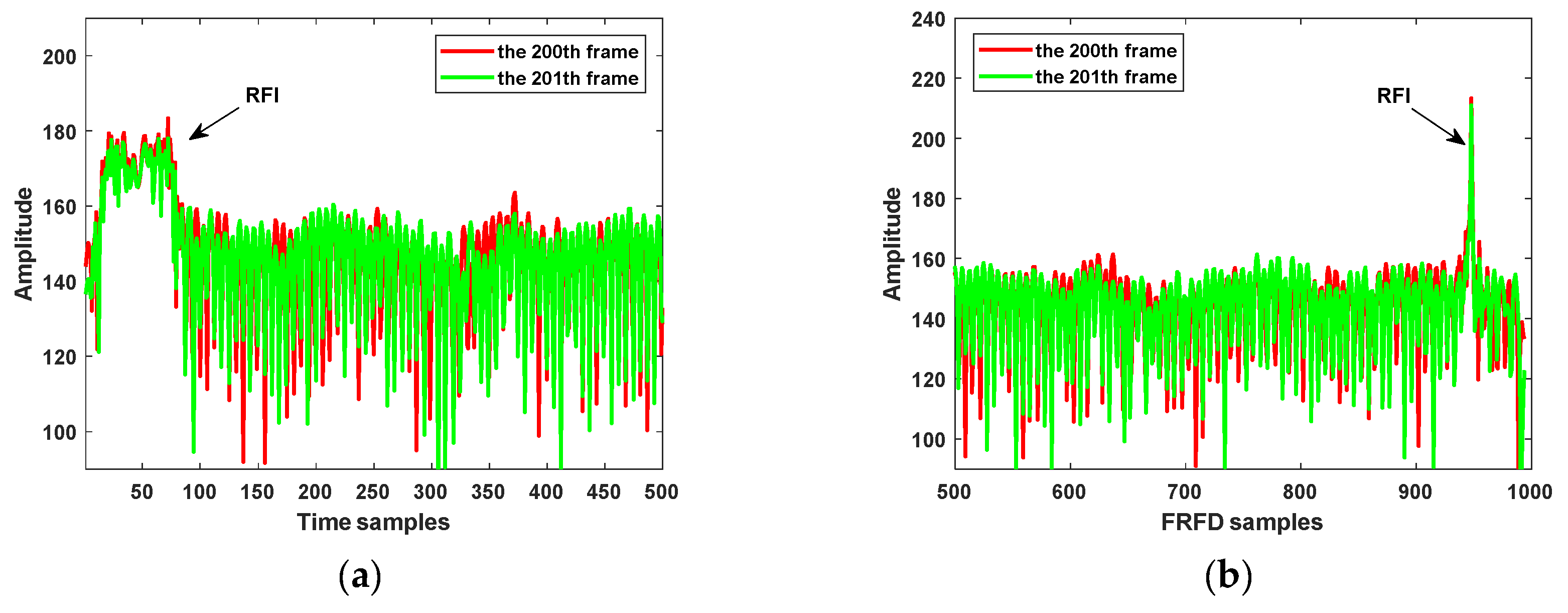
The carrier frequency of the simulated RFI in Case 1 was invariable, and the interference lasted for 600 sweep periods. The original signals perturbed by stationary RFI are shown in Figure 4a, of which the red line and green line represent time samples from the 200th and 201st sweep periods, respectively. Amplitude of interference was 20 dB higher than the echo. The time sequence was then transformed into FRFD (Figure 4b) with optimal matched-order $p_{opt}=1.9579$. As a result, interference was aggregated into impulses, and the peak amplitude was 50 dB higher than the echo. This aggregation effect of FRFT facilitated the detection and identification of RFI. Additionally, since the carrier frequency of simulated RFI was unvaried, the distribution of interference from different sweep periods remained the same in both time domain and FRFD. The RDS of original data with injected RFI is in Figure 5a. After range and Doppler processing, RFI turned into stripes that distributed from −0.2697 to −0.1692 Hz in Doppler, and spread to all range bins. The injected target located at −0.206 Hz, the preset direction of arrival (DOA) of which was 140° from the array direction. The target was buried by RFI and difficult to be detected. Figure 5b shows RFI-mitigated results with OP-FRFD algorithm proposed. Sampling data from the first 200 sweep periods was selected to calculate the interference covariance matrix. The added RFI was suppressed effectively, and sea echoes and the target were revealed. Figure 5c shows RFI-mitigated results with SVD-FRIFD algorithm, and sampling data of each sweep period was processed separately. The RFI was suppressed, and echo from the sea and target was reserved.

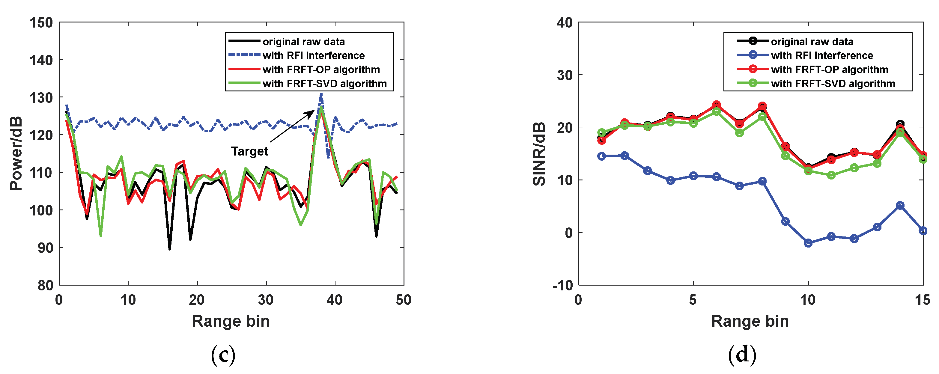
Doppler spectrums from the fifth (with sea clutter) and 37th (with target) range bin after RFI cancellation can be found in Figure 6a,b. The plus and minus first-order Bragg peaks remained unvaried with both methods, and signal-to-interference-plus-noise ratio (SINR) results of the target had a significant improvement from 3.2 dB to 11.5 dB with the OP-FRFD algorithm and to 10.0 dB with the SVD-FRIFD algorithm. Figure 6c shows spectrum of 50 range bins at −0.206 Hz in Doppler. The spectrum power for target remained high after processing, while interference in the background decreased obviously. The range spectrum with the SVD-FRIFD algorithm (the green line) was more constant with that of original (the black line), the root mean squared error (RMSE) was 0.11. While for the OP-FRFD algorithm (the red line), RMSE was 0.18. Figure 6d shows the SINR results of sea clutter for 15 range bins. Both methods effectively improved SINR, and the OP-FRFD algorithm yielded better SINR improvements than that of the SVD-FRIFD algorithm.

3.2. Case 2: RFI with Time-varying Carrier Frequency

The carrier frequency of the simulated RFI in Case 2 varied randomly between adjacent sweeps. The maximum variation was 50 Hz, and the interference lasted for 600 sweep periods. The original signals perturbed by nonstationary RFI are shown in Figure 7a (and then transformed into FRFD in Figure 7b), of which the red line and green line represent time samples from the 200th and 201st sweep periods, respectively. Due to the variation of carrier frequency, the distribution of interference from different sweep periods varied in both time domain and FRFD. Figure 8a shows RDS with injected RFI and target. Strips of interference nearly occupied all Doppler and spread to all range bins after the range and Doppler processing. Figure 8b shows RFI-mitigated results with the OP-FRFD algorithm. Sampling data from the first 200 sweep periods was applied to calculate the interference covariance matrix. As a result, most of the interference was suppressed, and sea echoes and target emerged. However, residual RFI still existed in −0.9 Hz, −0.5 Hz, −0.34 Hz, and 0.34 Hz in Doppler. Figure 8c shows RFI suppression results with SVD-FRIFD algorithm. Sampling data from each sweep period was processed separately. As a result, the added RFI was suppressed completely, the background in RDS was much clearer, and the sea echoes remained unchanged.

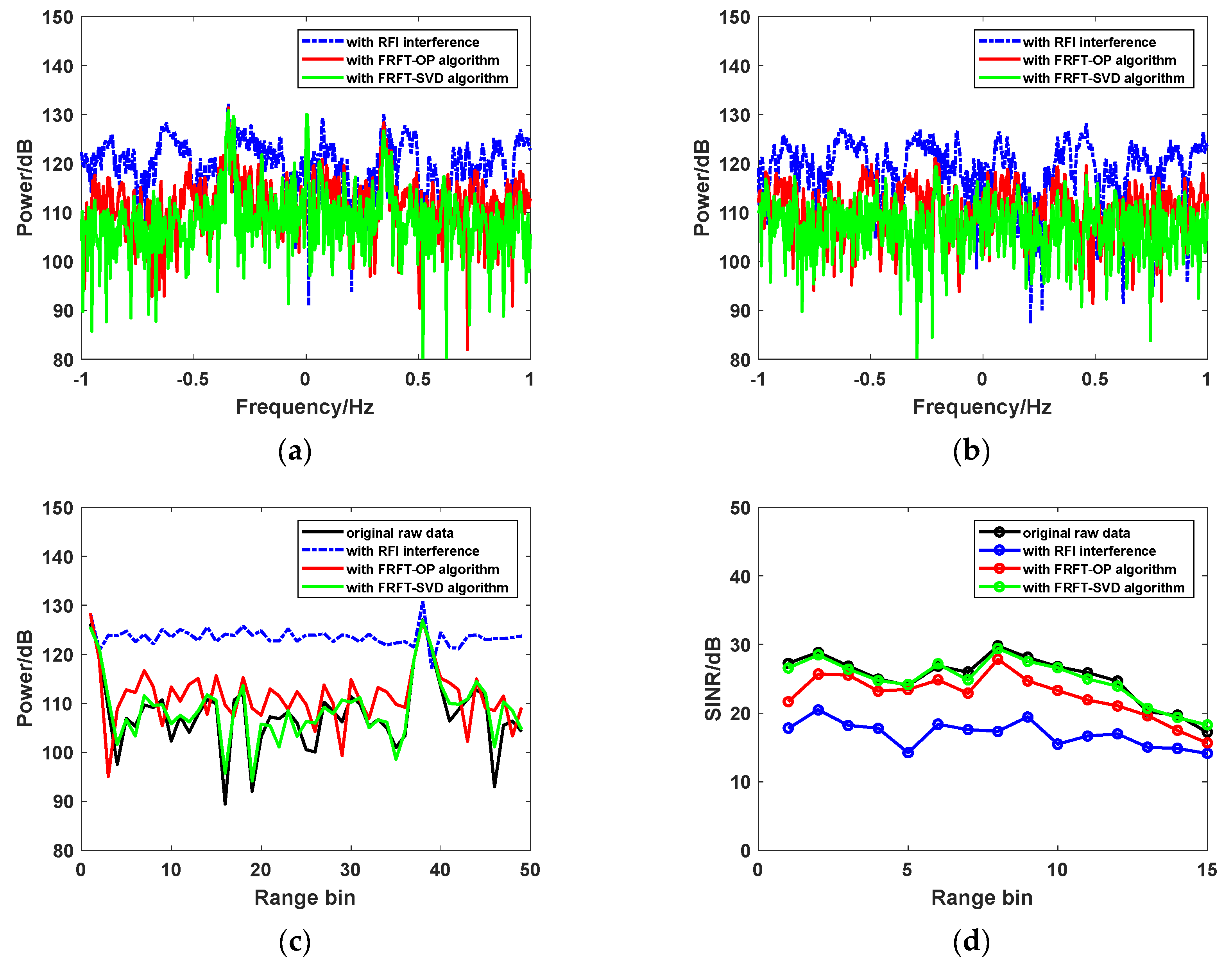
Figure 9a,b show Doppler spectrums from the fifth and 37th range bin after RFI suppression. The interference was more sufficiently suppressed with the SVD-FRIFD algorithm, and echoes from ocean and target remained unvaried. SINR of target had a significant improvement from 3.5 dB to 8.7 dB with the OP-FRFD algorithm and to 9.9 dB with the SVD-FRIFD algorithm. Figure 9c shows spectrum of 50 range bins at −0.206 Hz in Doppler. Spectrum power for target remained high after processing. The range spectrum for SVD-FRIFD algorithm was more constant with the original one, the RMSE was 0.08, and RMSE for the OP-FRFD algorithm was 0.17. Figure 9d shows the SINR results of sea clutter for 15 range bins. Both methods effectively improved SINR, and the SVD-FRIFD algorithm yielded bigger SINR improvements than that of OP-FRFD algorithm.

Figure 10 shows the angular response of the injected target before and after RFI mitigation using the multiple signal classification space spectrum estimation for both cases. The peaks of the mitigated results were 140° for the OP-FRFD algorithm and 141° for the SVD-FRIFD algorithm in Case 1, and in Case 2 was 142° for the OP-FRFD algorithm and 141° for the SVD-FRIFD algorithm. The mitigated results agreed well with the preset direction.

Table 1. SINR of target at −0.206 Hz in 37th range bin.

	Original (dB)	With RFI (dB)	OP-FRFD (dB)	SVD-FRIFD (dB)
case 1	11.4	3.2	11.5	10.0
case 2	11.4	3.5	8.7	9.9

is SINR of target in three cases.

Table 2. Root mean squared error (RMSE) of range spectrum between results after processing and that of original.

	With RFI	OP-FRFD	SVD-FRIFD
case 1	0.22	0.18	0.11
case 2	0.22	0.17	0.08

represents RMSE of range spectrum at −0.206 Hz between the original and that after processing. It is clear that, with the increasing of maximum RFI frequency variation between sweeps, the interference cancellation performance for the OP-FRFD algorithm degraded. This degradation arose from the decoherence of RFI in adjacent sweeps. The interference cancellation performance with the SVD-FRIFD algorithm kept steady. It is applicable for suppressing both the stationary and nonstationary interferences.

4. Experimental Results

The experimental data was collected at 3:43 LT on 28 December 2016. Both of the sites for transmitting and receiving were deployed at Chihu (24.04°N, 117.90°E) Fujian province, China, off the coast of the Taiwan Strait. Line array for receiving was composed of eight monopoles antennas, and the normal array direction was 137° referring to north. Some parameters of the HF SWR system were as follows: The center frequency was 13.15 MHz, the bandwidth was 30 kHz, the sweep period was 0.5 s, CIT was 300 s (including 600 sweep periods), a sweep period was composed of 996 snapshots, and range resolution was 5 km. For more details of the experimental HF SWR system, one is referred to literatures [23,24]. Figure 11a shows the power distribution of raw data transformed into FRFD, the optimal matched-order $p=1.958$. As we can see, external RFI constantly appeared for 530 sweep periods (from the 70th to 600th sweep periods) and the interference was gathered mainly in the 10th, 310th, and 620th sampling points. Figure 11b shows the power density spectrum of original data after the range and Doppler processing. As a result, external RFI was converted into a bunch of strips across all range bins; the interference mainly existed in −0.83 Hz, −0.43 Hz, −0.03 Hz, 0.36 Hz, and 0.76 Hz in Doppler; and useful signal such as sea echoes was masked. The original RDS in Figure 11b cannot be used for current inversion. As RFI generated spurious signals in RDS, they may be misinterpreted by the current and wave algorithm [24,29] as the first-order Bragg peak. As a result, patches of fake current within the expected range may cover the real current.

Figure 12a,b show the amplitude spectrum of original data from the 206th sweep period that processed with OP-FRFD algorithm and SVD-FRIFD algorithm, respectively. The dotted line is the threshold calculated, the scale factor $\eta =10\mathrm{dB}$, and the circles represent local maxima that identified as RFI. As a result, RFI was mitigated with both algorithms. Nevertheless, there was still residual RFI in the 167th sampling point with the OP-FRFD algorithm. By contrast, data sequence was more consistent with the original sequence after RFI mitigation with SVD-FRIFD algorithm, and there was no residual interference.

Figure 13a shows RDS after RFI cancellation with the OP-FRFD algorithm. Sampling data from the 70th to 600th sweep periods was used to estimate the interference covariance matrix. Interference was mitigated, in spite of residual interference still existing. Figure 13b shows RDS after RFI cancellation with the SVD-FRIFD algorithm. The method was employed sweep by sweep, and interference was totally cleaned up. For comparison, two previously proposed time-domain orthogonal projection schemes were applied to the experimental data. The first time-domain RFI cancellation scheme (referred to as time-domain Scheme 1)uses data on the range and sweep dimensions to estimate the interference covariance matrix, while the second time-domain RFI cancellation scheme (referred to as time-domain Scheme 2) estimates the interference covariance matrix with data on antenna channel and range dimensions. Figure 13c shows RDS after RFI cancellation with time-domain Scheme 1. Time-domain samples at clutter-free range bins (between 20 and 40) were used for interference training. Although interference at clutter-free range bins (between 20 and 40) was effectively suppressed, residual RFI still existed in range bins between 0 and 20 of the RDS. This is because the interference in the near range cannot be effectively orthogonal projected onto the interference subspace obtained by samples at clutter-free range bins. Figure 13d shows RDS after RFI cancellation with time-domain Scheme 2, and the interference training was implemented with samples of eight antenna channels at clutter-free range bins (between 20 and 40) in each sweep. RFI was suppressed completely, and the background noise was completely reduced. However, the separating processing of sequences from each sweep period brought about temporal decoherence, resulting in frequency spreading in the near range bins (between 0 and 5) of the RDS.

Doppler spectrums in the third range bin are presented in Figure 14a. Residual interference still existed in −0.85 Hz, 0 Hz, 0.77 Hz, and 0.95 Hz with time-domain Scheme 1 and OP-FRFD algorithm. Although interference was effectively mitigated with time-domain Scheme 2, there was frequency spreading which may cover up spectral points of real targets and severely increase the false alarm rate for target detection. Additionally, spurious signals generated in RDS may be misinterpreted by the current and wave algorithm, and deteriorate the accuracy of environmental remote sensing. By comparison, interference was suppressed completely and the sea clutter remained unvaried with the SVD-FRIFD algorithm. SINR results of plus Bragg peak for 11 range bins are presented in Figure 14b. The average increment of SINR for time-domain Scheme 1 was about 0.3 dB, while that increment for time-domain Scheme 2 was about 9 dB, for the OP-FRFD algorithm was about 2.7 dB, and for SVD-FRIFD was about 3.5 dB. Despite the time-domain Scheme 2 having the advantage of a higher SINR, the highly spreading frequency components of both first- and second-order Bragg returns may severely degrade the application prospects of the algorithm for surveillance and environmental remote sensing. The SINR results suggest that the SVD-FRIFD algorithm yielded better SINR improvement than the OP-FRFD algorithm after RFI cancellation. Compared with the traditional time-domain orthogonal projection methods, the proposed OP-FRFD algorithm and SVD-FRIFD algorithm are more applicable for RFI suppression of HF SWR.

5. Discussion

The OP-FRFD algorithm proposed utilized correlation of RFI between sweep periods, and was only applicable for suppressing interferences with unvaried carrier frequency (or the carrier frequency was limited to a narrow bandwidth that can be neglected) within the time of appearance. In practice, however, most RFIs do not meet this requirement, resulting in poor cancellation performance. Additionally, echo of direct wave and terrestrial clutter may also possess great correlation. In this circumstance, the largest several singular values contained most of the power of the interferences as well as echo of direct wave and terrestrial clutter. Both the external RFI and echo of direct wave and terrestrial clutter will be mitigated after the orthogonal projection. This was unfavorable for situations when direct wave was required for array calibration. The criterion for selecting singular values corresponding to interference subspace needs to be explored in the future.

In contrast, the SVD-FRIFD algorithm proposed was capable of suppressing both stationary and nonstationary RFI as long as the carrier frequency of the interference was invariant or limited to a narrow bandwidth during the sweep period. Since the time cost for Hankel matrix decomposition with SVD is relatively high, the capability of this method for batch processing is severely limited. Accordingly, the applicability of the method for surveillance is inferior to that for environmental remote sensing (such as sea state monitoring), since HF SWR used for environmental remote sensing requires a relative longer CIT to achieve a higher frequency resolution. When ignoring the high computational time consumption of the SVD decomposition, the RFI cancellation effect of the proposed SVD-FRIFD algorithm is equally good for HF SWR used for environmental remote sensing and surveillance. Additionally, the column number of the Hankel matrix exerted great impact on the inhibition results and needs to be carefully selected. Specifically, a too-small or an oversized $P$ may both make it difficult to divide interferences and useful signal with SVD, causing attenuation of useful signal or leaving residue interference after RFI suppression procedure.

For cases when carrier frequency of RFI changes so rapidly that it cannot be recognized as unvaried during a sweep circle, the interference was unable to be effectively aggregated by FRFT and was difficult to be detected with the proposed threshold method. A valid approach is to divide snapshots from a single sweep circle into several segments and to process sampling sequence in each segment separately. The price with this approach is the decline of signal resolution in FRFD.

6. Conclusions

Some conclusions are as follows:

External RFI can be recognized as the combination of a finite number of single-frequency components. When mixed with LO and passed through a low-pass filter, external RFI is translated into chirp signals with identical chirp rate to LO. FRFT is the decomposition of chirp bases and thus is an ideal tool for analyzing RFI. With the threshold method proposed, it is possible to accurately determine whether RFI exists and where it locates in FRFD. The distribution of stationary RFI in FRFD is nearly consistent. By contrast, the distribution of nonstationary RFI in FRFD is much more stochastic.

The OP-FRFD algorithm proposed in this article calculates the interference covariance matrix with data sequences from FRFD frequency-sweep two-dimension plane, and is efficient for suppressing RFI with strong correlation in FRFD. The interference suppression performance decreased with the increase of maximum carrier frequency variation of RFI. Compared with traditional orthogonal projection algorithm using information about the antenna channel dimensions, the OP-FRFD algorithm was not limited by insufficient degree of freedom, and is applicable for mitigating RFI with multiple components.

The key for RFI suppression with SVD-FRIFD algorithm is that interferences aggregated in FRFD can be regarded as a finite number of narrow-band signals, and Hankel matrix decomposition with SVD is an efficient way to reconstruct the interference subspace. Compared with the OP-FRFD algorithm, SVD-FRIFD algorithm achieved a firm interference mitigation performance for both the stationary and nonstationary RFI, and is more applicable in practical use. Nevertheless, the time cost for Hankel matrix decomposition with SVD is relatively high, which restricts the capability of this method for batch processing. What is more, the selection of column number P exerted great impact on the interference suppression results.

Both of the FRFT-based algorithms proposed are applicable for compact HF SWR with small-aperture array, and are valid for suppressing multicomponent interferences with the premise that the carrier frequencies of RFI remain unvaried within a sweep circle. For cases when the carrier frequencies of interferences vary so dramatically that they cannot be well accumulated by FRFT, an approach by segmenting the original data sequence and processing each part, respectively, can be implemented.

The FRFT-based RFI cancellation algorithms proposed took advantage of the prior knowledge that RFI presents as chirp signals in each sweep period after entering the receiver, and the aggregation characteristic of FRFT for chirp signals offered a critical condition to detect RFI with small magnitude. Additionally, we constructed a covariance/Hankel matrix with sequences in FRFD, and used SVD to decompose the matrix to suppress RFI. Compared with traditional spatial adaptive beamforming schemes based on large arrays, the proposed FRFT-based algorithms were more applicable for compact HF SWR, and can provide a better cancellation performance for multiple interferences. Both simulation and experimental results demonstrated the feasibility and effectiveness of the methods. The comparison with traditional time-domain orthogonal projection methods proved that the proposed FRFT-based algorithms could significantly suppress RFI without the frequency spreading of the spectrum. The algorithms proposed in this paper provide a novel approach for HF SWR RFI suppression. The results of the paper provide significant evidence for further development of the FRFT-based RFI suppression algorithms for HF SWR.

Although some positive results have been obtained, it must be pointed out that the algorithms are still not yet perfect. The distinction between time-invariant and the time-varying carrier frequency is of great limitation. The criterion for selecting the number of interference vectors for the OP-FRFD algorithm is still vague. The computational time consumed for the SVD-FRIFD algorithm is still intolerable. By selecting a shorter column number of the Hankel matrix, we can diminish the time cost of the SVD decomposition. However, this will inevitably degrade the performance of interference suppression. Future work will focus on finding more precise criteria to construct the interference subspace and to find a more applicable way to reduce the time cost of Hankel matrix decomposition with SVD.