How Hyperspectral Image Unmixing and Denoising Can Boost Each Other


1
Helmholtz-Zentrum Dresden-Rossendorf, Helmholtz Institute Freiberg for Resource Technology, Machine Learning Group, Chemnitzer Straße 40, 09599 Freiberg, Germany
2
Imec-Visionlab, University of Antwerp (CDE) Universiteitsplein 1, B-2610 Antwerp, Belgium
*
Author to whom correspondence should be addressed.
Remote Sens. 2020, 12(11), 1728; https://0-doi-org.brum.beds.ac.uk/10.3390/rs12111728
Submission received: 30 March 2020
/
Revised: 25 May 2020
/
Accepted: 26 May 2020
/
Published: 28 May 2020
(This article belongs to the Special Issue Remote Sensing Applications of Image Denoising and Restoration)
Abstract
:Hyperspectral linear unmixing and denoising are highly related hyperspectral image (HSI) analysis tasks. In particular, with the assumption of Gaussian noise, the linear model assumed for the HSI in the case of low-rank denoising is often the same as the one used in HSI unmixing. However, the optimization criterion and the assumptions on the constraints are different. Additionally, noise reduction as a preprocessing step in hyperspectral data analysis is often ignored. The main goal of this paper is to study experimentally the influence of noise on the process of hyperspectral unmixing by: (1) investigating the effect of noise reduction as a preprocessing step on the performance of hyperspectral unmixing; (2) studying the relation between noise and different endmember selection strategies; (3) investigating the performance of HSI unmixing as an HSI denoiser; (4) comparing the denoising performance of spectral unmixing, state-of-the-art HSI denoising techniques, and the combination of both. All experiments are performed on simulated and real datasets.

1. Introduction
Hyperspectral unmixing is considered as one of the main analysis tasks on hyperspectral datasets [1]. Hyperspectral images (HSI) contain detailed spectral information, compromising the spatial resolution. Because of this, HSI pixels often contain mixtures of several materials. Due to the uniqueness of the materials’ spectral signatures, spectral unmixing reveals which materials are contained within a pixel and their fractions. The most widely applied spectral mixing model is the linear model, which assumes that a light ray only interacts once with a material before reaching the sensor. It describes a reflectance spectrum as a linear combination of the pure material spectra (endmembers), and the coefficients are the fractional abundances of the endmembers. Many methods have been developed for (1) estimating the number of endmembers, (2) obtaining the endmembers, and (3) estimating the fractional abundances.
In this work, we will assume that the number of endmembers is known a priori. Different strategies are applied to obtain endmembers. One strategy is to extract the endmembers from the data as pure pixels. Examples are geometric methods that look for the outer boundary points of the data manifold, e.g., the vertices of a simplex [2]. In highly mixed scenarios, no pure pixels may be available, and the endmembers need to be estimated, e.g., by describing the minimum volume simplex that enclosed the data [3,4,5,6]. Finally, endmembers can also be selected from available spectral libraries. Several library-based methods incorporate different types of sparsity to limit the number of endmembers that a mixture can contain [7,8,9].
The most popular abundance estimation method is fully constrained least squares unmixing (FCLSU) [10,11], which minimizes the error between the observed spectrum and the linear model, subject to the physical constraints that the abundances should be positive and sum to one. Other methods estimate the endmembers and the abundances simultaneously, e.g., by nonnegative matrix factorization procedures [3,4,5,6].
When higher-order interactions and intimate mixing play a role, the linear model is no longer valid. Many nonlinear solutions for hyperspectral unmixing have been proposed. Nonlinear unmixing falls outside of the scope of this work.
On the other hand, noise plays an important role in HSIs. Radiance measured at the sensor is degraded by two main sources, i.e., atmospheric and instrumental effects. After applying atmospheric corrections on the radiance, reflectance, which represents the physics of the material, is obtained. Instrumental noise including thermal, quantization, and shot noise can considerably affect the reflectance. Spectral bands can be highly corrupted, which leads to the loss of information in the corresponding wavelengths. These corrupted bands degrade the efficiency of the HSI analysis techniques, and therefore, they are often removed from the data before any further processing. Alternatively, HSI denoising improves the SNR of the HSI and therefore the further analysis of HSI [12]. The Gaussian noise removal techniques developed for HSI can be divided into three main groups. The first group contains methods that use 3D models and 3D filtering approaches. Those techniques exploit 3D models to describe the noise and the signal both spatially and spectrally and then apply filtering steps to remove the noise from the signal. For instance, in [13], the discrete Fourier transform (DFT) and the 2D discrete wavelet transform (2D DWT) were applied spectrally and spatially, respectively, for denoising the HSI signal. In [14], a 3D blockwise nonlocal sparse HSI denoising was proposed. In [15], the use of 3D (undecimated) wavelets and sparse regularization was proposed for HSI denoising. The second group contains spectral penalty-based approaches that incorporate penalties to exploit the high spectral correlation of HSI. A first order spectral roughness penalty was suggested for a penalized least squares method [16] to exploit the high spectral correlation in HSI. It has been shown that combining a spatial penalty with a spectral one can improve the performance of those techniques [17,18,19]. The third group contains the techniques based on low-rank modeling, which assumes that an HSI lives in a low spectral dimension. However, this dimension or the rank of the subspace (which is equal to the number of endmembers) is hard to estimate [20,21]. Parallel factor analysis (PARAFAC) [22], sparse reduced-rank restoration (SRRR) [23,24], wavelet-based reduced-rank regression (WSRRR) [25], low-rank total variation (LRTV) regularization [24,26], and automatic hyperspectral restoration (HyRes) [27] are all low-rank hyperspectral noise reduction techniques. It has been shown that the low-rank methods outperform the other techniques in terms of SNR [12]. Additionally, some techniques assume mixed noise in HSI. In [28], a technique was proposed to remove Gaussian and Poisson noise sequentially using maximum likelihood estimation of the model parameters. Sparse and low-rank decompositions have been widely used for mixed Gaussian and sparse noise reduction in HSI [29,30]. Recently, a sequential technique was proposed for the removal of mixed Gaussian and sparse noise [31]. In this paper, we only consider Gaussian noise, while other types of noises are left for future studies.
Although a large number of HSI denoising techniques have been developed, only a few of those works considered denoising as a preprocessing step for spectral unmixing. In [32], denoising was performed to improve the endmember extraction. In [33], the noisy and water absorption bands were denoised and included in the data to improve a sparse spectral unmixing technique. In [34], a denoising constraint was incorporated in an unsupervised auto-encoder model for spectral unmixing. In [35], the spectral unmixing process was formulated in such a way that it accounted for mixed Gaussian and sparse noise.
On the other hand, some works studied the use of linear unmixing as a denoiser. Most of these works concluded that spectral unmixing is an effective denoiser, when employing low-noise endmembers, e.g., extracted from class averages from ground truth information [36], from homogeneous regions [37], or by providing library endmembers in a spatial-spectral library-based spectral unmixing technique [38]. Some algorithms were developed to perform denoising and unmixing jointly in a unified framework, with the purpose of improving both. Both in [39,40], sparse representation frameworks were developed, where denoising and unmixing acted as constraints of each other. In most of the aforementioned studies, the performed experiments were small scale and rather anecdotal in nature. In this work, a more general study on the effect of noise and denoising on the process of hyperspectral unmixing is pursued.
Contribution
In this paper, we do not propose new algorithms either for HSI unmixing or for HSI denoising. The main contribution of the paper is to perform an extensive experimental study on the influence of Gaussian noise on the process of hyperspectral linear unmixing. In particular, experiments will be conducted to:
- investigate the effect of HSI denoising as a preprocessing step on the performance of spectral unmixing.
- study the relation between noise and unmixing for different strategies of obtaining endmembers.
- investigate the performance of spectral unmixing as a denoiser.
- compare the denoising performance of spectral unmixing with a number of state-of-the-art denoising techniques.
- study the effect of colored versus white noise on all the above research.
Experiments were performed on one simulated and two real HSI datasets. Both white and colored noise situations with a wide range of SNR values were investigated. The study is comprised of four different strategies for obtaining endmembers and three state-of-the-art denoising methods.
In this paper, we considered remote sensing datasets; however, the discussions and conclusions are valid for all types of HSI datasets.
2. Hyperspectral Unmixing
In this section, we describe the theory behind spectral unmixing. We assume that an HSI is linearly modeled as:
where Y, X, and N (all ) denote the observed HSI, the noise-free HSI, and the noise in the HSI, respectively. p and n indicate the number of spectral bands and pixels, respectively. In spectral unmixing, (1) is rewritten as:
where E () and A () are low-rank matrices (i.e., ), respectively containing the endmembers and abundances of the HSI. r denotes the number of endmembers. Unmixing is the problem of separating the abundance fractions A from the endmember sources E in the mixing model (2). We will discuss the three relevant strategies of the unmixing problem and consequent algorithms: (1) abundance estimation methods that are supervised, i.e., that assume that the endmember spectra of the pure materials are provided; (2) methods that extract or estimate the endmembers from the data; and (3) blind methods that estimate the endmembers and abundances simultaneously. We should mention that the selection of the number of endmembers (or the dimension/rank of the subspace) is also an important topic, which is often discussed in relation to noise, and for this, we refer to [20,21]. Additionally, model (2) is often used for hyperspectral supervised/unsupervised feature extractions as well [41].
2.1. Fractional Abundance Estimation
With known endmembers, the goal of unmixing is to estimate the matrix , with columns ), that has the highest probability of representing , with columns ), through the linear mixing equation under the noise model. When assuming uncorrelated Gaussian noise with zero mean for each band and covariance matrix I, where I is the identity matrix, the maximum-likelihood estimation of the abundance vector of each pixel (we will omit the subscript i) is given by:
where is the probability of observing for a given and :
where the value is the mth component of and represents the abundance value of endmember m, is band j of , and is band j of endmember m. Hence:
Equation (5) shows that the solution of Equation (2) is the least squares approximation. Because the fractional abundance is the volume percentage, it is assumed that no endmember can have a negative volume, yielding the abundance nonnegativity constraint (ANC), and that the observed spectrum is completely decomposed by endmember contributions, leading to the abundance sum-to-one constraint (ASC). Unfortunately, least squares solutions do not obey ASC and ANC. To obey both constraints, the fully constrained least squares unmixing algorithm (FCLSU) has been developed [10,11]. It minimizes s.t. , .
2.2. Endmember Extraction
When the endmembers are not provided, they have to be estimated from the data. In the noiseless case, i.e., when N = 0, the hyperspectral dataset that follows the fully constrained linear mixing model lies within a (r − 1)-dimensional simplex of which () are the vertices or extreme points. This inspired many methods and algorithms that effectively search for embedding or enclosing simplices in the data ([2]). For example, NFINDR randomly selects a set of r pixels from the dataset as initial endmembers and iteratively updates the endmembers at each time, replacing an endmember by a pixel from the dataset to find the largest volume simplex. The volume is calculated as:
because the matrix in (6) is non-square, linear dimensionality reduction is commonly applied to reduce the data to dimension r − 1.
Instead of reducing the dimensionality of the dataset, in [42], Equation (6) was reformulated by expressing the volume of a simplex via inter-vertex distances, by exploiting the Cayley–Menger determinant ():
where is the Euclidean distance between endmembers and . In this paper, we will use this algorithm to extract endmembers from the dataset and refer to it as the simplex volume maximization technique (SiVM).
2.3. Simultaneous Estimation of Abundances and Endmembers
When no pure spectra are available in the dataset, the extracted endmembers by applying SiVM are in themselves mixtures of pure spectra. To solve this problem, the work in [43] provided a criterion to estimate endmembers for non-pure pixel case scenarios. The main idea is that endmembers can be estimated as the vertices of a minimum-volume simplex that encloses the dataset. Based on this criterion, several nonnegative matrix factorization (NMF) algorithms have been proposed to estimate the endmembers along with the fractional abundances, such as the minimum-volume enclosing simplex algorithm [5], volume-constrained nonnegative matrix factorization (MVCNMF) [3], minimum volume simplex analysis [4], and collaborative nonnegative matrix factorization (CoNMF) [6]. In particular, when the number of endmembers is known a priori, CoNMF estimates E and A by solving the following optimization problem:
where is a regularization parameter and is the mean value of the data. The regularization term on the endmembers pushes them toward the dataset mass center, thus promoting a minimum volume enclosing simplex.
3. Hyperspectral Denoising
Denoising is the problem of estimating X based on the observation Y. Hyperspectral denoising was comprehensively discussed in [12]. From a modeling point of view, linear HSI denoising can be divided into two main groups; techniques that are developed based on either low-rank models or full-rank models. Differences between those models were discussed in [24]. In this paper, we employ the full-rank model-based method first order spectral roughness penalty denoising (FORPDN) [16], the low-rank model-based HyRes [27], and the conventional multiple linear regression technique (MLR) [21]. All three methods are discussed below.
3.1. Multiple Linear Regression
To exploit the high correlations between spectral bands, the work in [21] suggested to apply multiple linear regression to estimate the noise in hyperspectral data. MLR assumes that each spectral band j is a linear combination of the other bands:
where is the data matrix excluding band j and assuming is the jth row in matrix . The regression vector () is estimated by using least squares:
Therefore, the noise in spectral band j is estimated as:
3.2. First Order Spectral Roughness Penalty Denoising
FORDPN [16] uses the full rank model (1) where and contains the two-dimensional (2D) wavelet bases. To estimate the wavelet coefficients , FORPDN solves the following minimization problem:
where is the noise covariance matrix, is a difference matrix, and is automatically selected using Stein’s unbiased risk estimate (SURE) [44], dependent on the decomposition level of the wavelets, l (), utilizing the multiresolution analysis property of the wavelet decomposition. Let , then Problem (10) can be solved for every wavelet decomposition level separately, and the solution is given by:
where are the wavelet coefficients of belonging to the decomposition level l, which are located at the ith column of matrix .
3.3. HyRes: Automatic Hyperspectral Restoration
HyRes [27] utilizes a low-rank model similar to (2) where in (1) is given by and () and and () are low-rank matrices. Here, contains the first r left-singular vectors of the observed signal . HyRes estimates by minimizing:
where the penalty term is applied on the low-rank matrix and is the jth row in matrix . Assuming , the solution to Problem (12) is given by:
4. Experimental Setup
4.1. The Data
4.1.1. Simulated Dataset
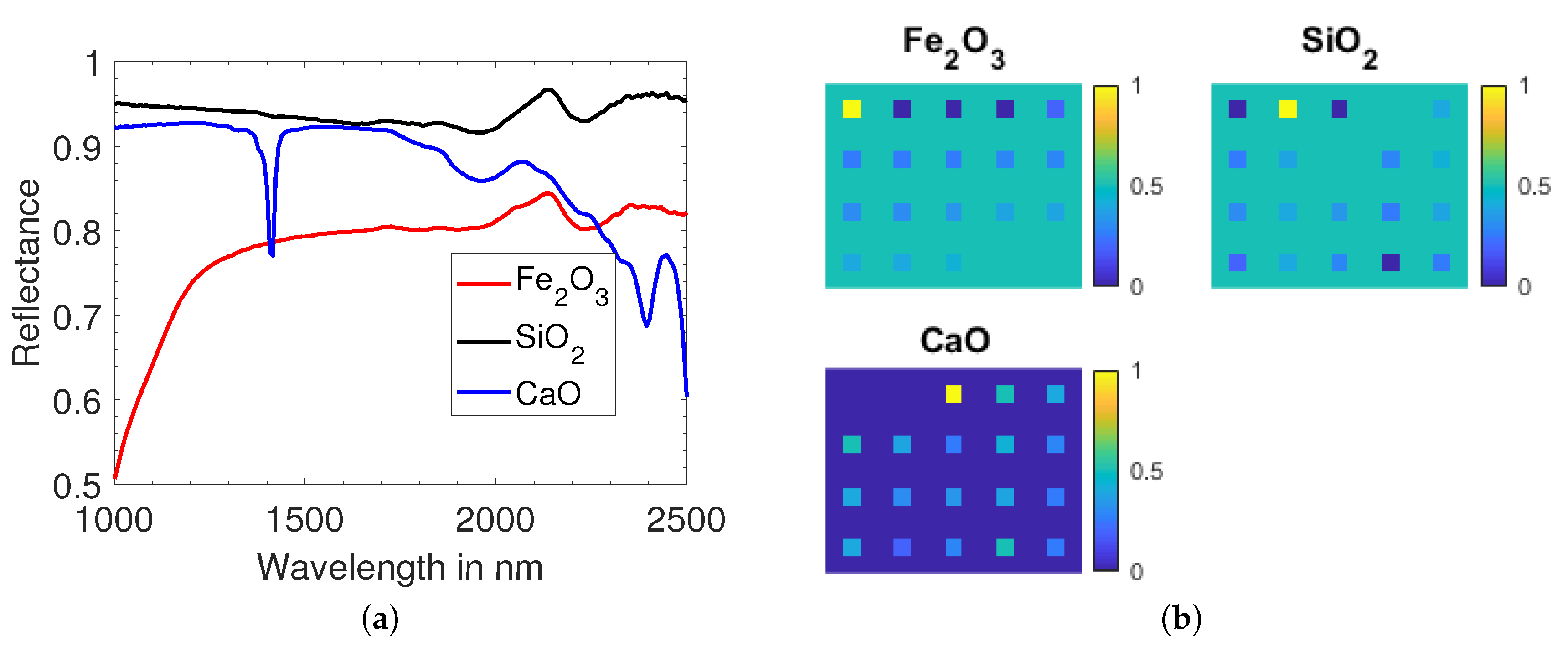
An HSI of 60 × 75 pixels was simulated, by making linear combinations of 3 minerals, i.e., Fe2O3, SiO2, and CaO. The endmembers of these minerals were measured by an AgriSpec spectrometer (manufactured by ASD (Analytical Spectral Devices)). These endmembers contained 200 reflection values in the wavelength range [1000–2500] nm. Figure 1a depicts the endmembers. Twenty squares of 5 × 5 pixels were generated with different binary and ternary linear mixtures. The remaining background contained binary mixtures of 50% of Fe2O3 and 50% of SiO2. The obtained ground truth fractional abundances are shown in Figure 1b.
4.1.2. Samson Image
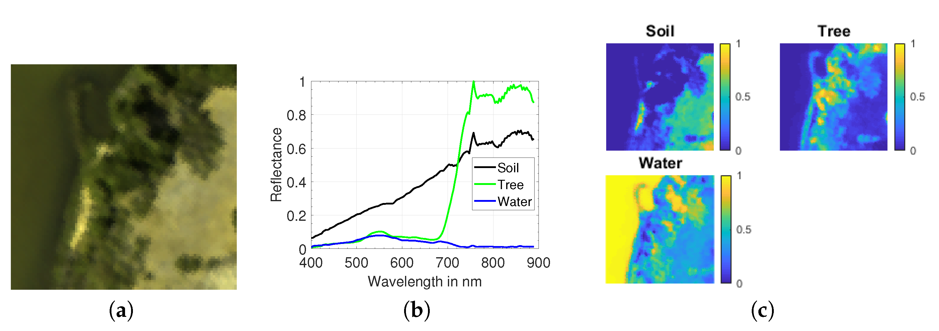
This image [45] contained 95 × 95 (9025) pixels. Each pixel spectrum contained 156 reflection values in the wavelength range [401–889] nm. In this image, there were three materials (soil, tree, and water). Pure spectra of these three materials were extracted by applying SiVM. Figure 2b displays the endmembers. Ground truth fractional abundances (see Figure 2c) were produced by applying FCLSU.
4.1.3. Jasper Ridge Image
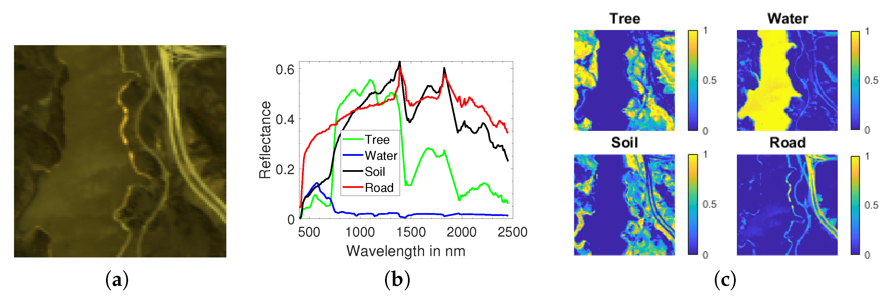
This image contained 100 × 100 pixels [45]. Each pixel spectrum contained 224 bands in the wavelength range [380–2500] nm. After removing 26 water absorption bands, one-hundred ninety-eight channels remained. In this dataset, there were four endmembers (tree, water, soil, and road). We applied SiVM and FCLSU to extract endmembers (see Figure 3b) and to produce the ground truth fractional abundances (see Figure 3c).
4.2. The Noise
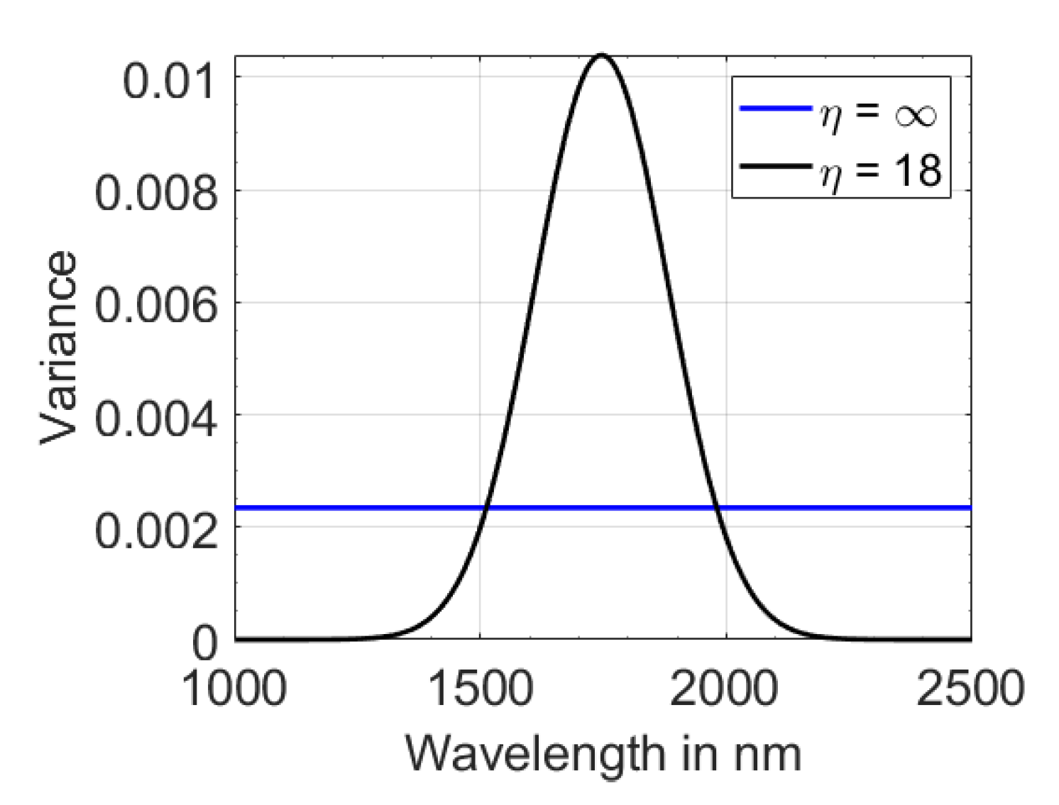
The Gaussian noise is simulated in a way that the noise variance of the spectral bands varies as:
where the power of the noise is centered at the middle band () and is controlled by and [21]. In this paper, we considered two noise scenarios, corresponding to two different values for : (1) the white noise scenario, ; in this case, the noise variance was the same for all bands; (2) the color noise scenario, ; for small values of , the noise variance changed from band to band according to a Gaussian-like shape with a small width (see Figure 4). The parameter was set to vary the image SNR between 10 dB and 50 dB with 5 dB intervals. This way of noise simulation was chosen to mimic that in HSI, the noise variance varies throughout the bands and that noise (as well as the signal) is correlated between neighboring bands [24]. In reality, the highest noise variance is not situated in the middle band, but it is a common practice in the literature to vary the noise variance in this way. Figure 4 shows how the noise variance varies along the spectral bands for and when SNR = 25 dB. We remark that the denoising methods in this work employed the noise correlations between the band and that the unmixing algorithms all involved the use of Euclidean distances between spectra, an abelian operation with respect to the order of the spectral bands.
4.3. The Endmembers
To obtain the endmembers, four different strategies, corresponding to different real scenarios, were applied.
4.3.1. Ground Truth Endmembers
In this scenario, it was assumed that the materials that occurred in the data were known and that their endmembers were provided. Only the abundances needed to be estimated. For this, we applied FCLSU. The endmembers could be the actual endmembers or they could be obtained as average spectra from ground truth class information, or homogeneous regions, or libraries. In all cases, the endmembers were expected to be noiseless or only contained low amounts of noise. In this work, we employed the ground truth endmembers that were provided with the data. This scenario was the ideal situation, where all endmembers were noise-free, and each material was represented by one unique endmember spectrum. In reality, this was hardly the case, and this scenario would be applied as a proof of concept.
4.3.2. Extracted Endmembers
In this scenario, the endmembers were extracted from the data, prior to unmixing. For this, we employed the SiVM algorithm. Then, FCLSU was applied to estimate the abundances. Since the data were noisy, the endmembers would be as well. Moreover, it was not guaranteed that each material in the data would be represented by a unique endmember. This was a realistic spectral unmixing scenario, in which no ground truth information about the materials was available. A prerequisite was that the data contained pure pixels for each of the materials.
4.3.3. Library Endmembers
In this scenario, it was assumed that a library of endmembers was available that included the reflectance spectra of the materials that occurred in the data. Again, SiVM was applied, and the obtained pure spectra were matched to the library endmembers in such a way that the closest endmember in terms of MSE would be chosen to represent the pure pixel. In this scenario, the endmembers would be noiseless, but not all materials may be presented by an endmember. Again, it was assumed that pure pixels were present in the data to represent each of the materials. In our experiments, we generated libraries by scaled versions of the actual ground truth endmembers. For this, each endmember was scaled 100 times with a varying factor between 0.5 and 1.5, with a step size of 0.01. For the unmixing, FCLSU was applied.
4.3.4. Estimated Endmembers
In highly mixed scenarios, the data contained no pure pixels, so that endmember extraction method would not work. In that case, one has to rely on methods that simultaneously estimate the endmembers and the fractional abundances. In our experiments, we applied the CoNMF algorithm. This situation was even harder than in the second situation. There was no guarantee that each material was represented by an endmember. The estimated endmembers would be smooth, however. Since the CoNMF algorithm required an initial estimate of the endmembers and the abundances, in our experiments, we tried several, including the endmembers from the three other scenarios, as initial values for the endmembers, and found the results to be quite insensitive for these initial choices.
4.4. The Experiments
We performed two groups of experiments.
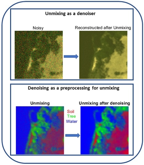
4.4.1. Denoising as Preprocessing for Unmixing
In the first experiments, we investigated the effect of denoising as a preprocessing step to improve the spectral unmixing performance. For this, the noisy images were denoised using the three denoising methods MLR, HyRes, and FORPDN, respectively. Then, the denoised images were unmixed using the four endmember strategies, respectively. This was compared to the direct unmixing of the noisy images. After unmixing, the reconstructed image was generated by multiplying the endmember matrix with the estimated abundance matrix. A quantitative comparison was provided by the reconstruction error (RE) and the abundance RMSE.
The reconstruction error is defined as the RMSE between the reconstructed image and the image on which the unmixing is performed (i.e., the noisy image if no preprocessing is performed or the a priori denoised image):
The abundance RMSE is defined as the RMSE between the estimated abundance matrix and the ground truth abundance matrix :
4.4.2. Unmixing as a Denoiser
In the second group of experiments, we investigated the denoising performance of spectral unmixing. For this, we performed spectral unmixing of the noisy images, using each of the four endmember strategies, respectively. From the endmembers and estimated abundances, an image was reconstructed. The results were compared to the three denoising algorithms MLR, HyRes, and FORPDN. Moreover, a combination of a denoiser with spectral unmixing was performed as well, to investigate whether spectral unmixing could improve the performance of a denoising algorithm for the purpose of denoising. A quantitative comparison was provided by the spectral RMSE, defined as the RMSE between the obtained reconstructed denoised image and the original noise-free image :
All experiments were repeated 20 times, and the average results are given. The standard deviations are shown by the error bars.
5. Simulated Dataset Experiments
5.1. Denoising as Preprocessing for Unmixing
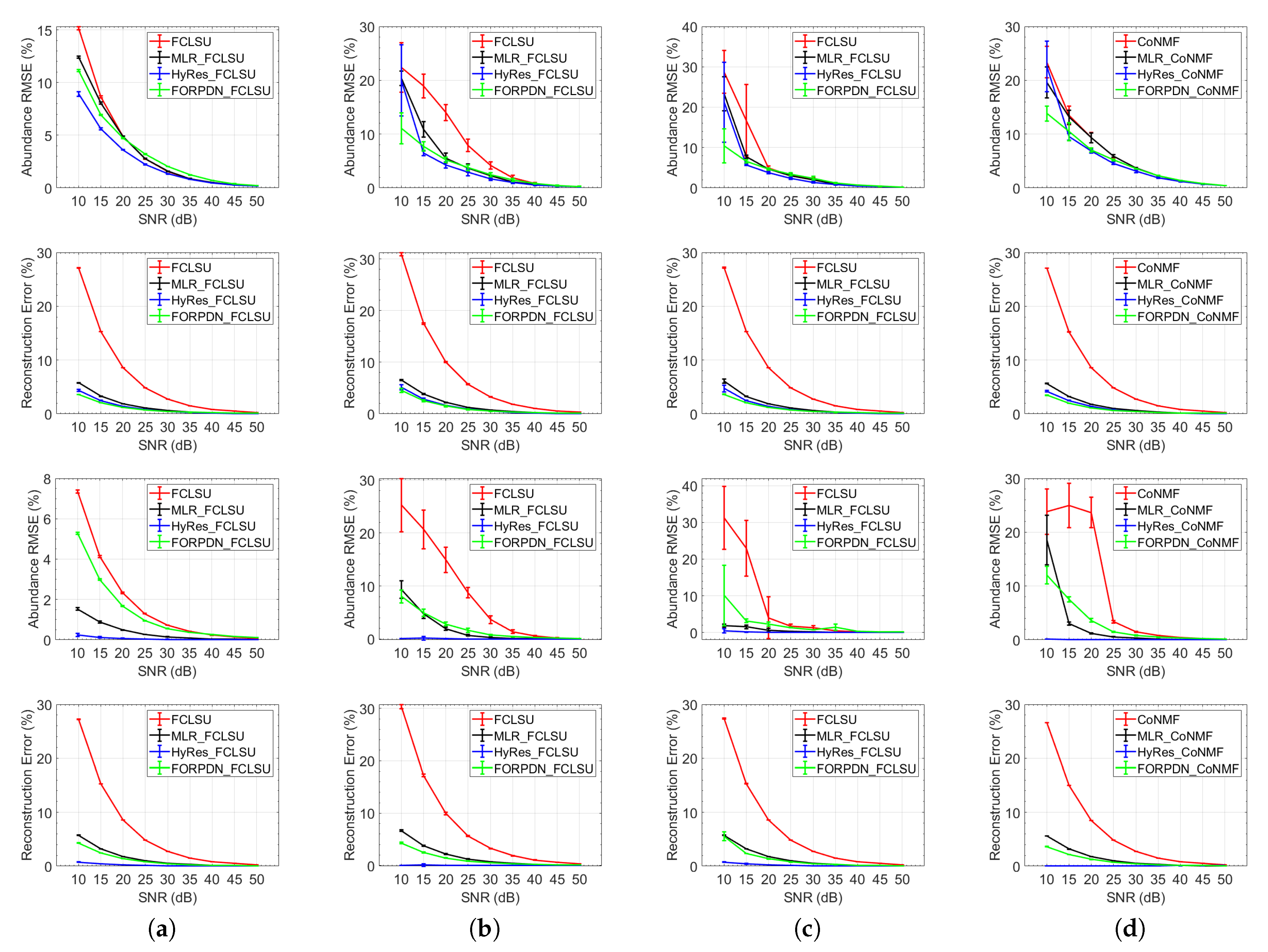
Here, the effect of the denoising techniques MLR, FORPDN, and HyRes as a preprocessing step on the performance of HSI unmixing was investigated. The denoising techniques were applied prior to the unmixing. Results for all four scenarios (i.e., (a) ground truth endmembers, (b) extracted endmembers, (c) library endmembers, and (d) estimated endmembers by using CoNMF), in terms of abundance RMSE and the reconstruction error, are shown in Figure 5. The red plots are the unmixing performances when no denoising was applied. The outcomes of the experiments are summarized as follows:
- Overall, one could observe the advantage of denoising as a preprocessing step for spectral unmixing. In general, the effects were minor for very high SNR and gradually increased when lowering the SNR.
- The largest improvements were observed on the reconstruction errors. This could be observed for all endmember strategies. Even for an SNR as high as 40 dB, this improvement was clearly observable.
- However, the performance on the abundance estimation did not improve proportionally. One could conclude that in noisy images, abundances were estimated reasonably well, irrespective of the high reconstruction errors, and that the spectral unmixing performance was not that much affected by the noise.
- When no denoising was performed (i.e., the red plots), the results with ground truth endmembers were superior (we should point out the different vertical scales in the graphs, which were selected to achieve a better visualization). From the other strategies, the one where endmembers were extracted performed the worst. The use of library endmembers performed well down to 20 dB, below which the abundance errors and the standard deviations became very large. We observed that at these noise levels, wrong endmembers were selected from the libraries. Furthermore, when endmembers were estimated, spectral unmixing performed worse for low SNR.
- In general, spectral unmixing performed worse with colored noise, compared to white noise, except when ground truth endmembers were available.
- After denoising, the performance of the abundance estimation generally improved. This was most obvious in the case of extracted endmembers, where better results were obtained with noise levels on the observed image up to 35 dB. In the case of colored noise, the improvements were more prominent than with white noise.
- In the case of white noise, MLR had the worst performance, and HyRes performed slightly better than FORPDN. Only for very low SNR, FORPDN performed better in all strategies, but the one with ground truth endmembers.
- In the case of colored noise, FORPDN was least performant, and MLR performed slightly better than FORPDN. HyRes showed by far the best performance for all endmember scenarios and all SNRs. The abundances were estimated almost correctly. This result strongly encouraged the use of a well-established low-rank denoising technique as a preprocessing step for unmixing.
5.2. Unmixing as a Denoiser
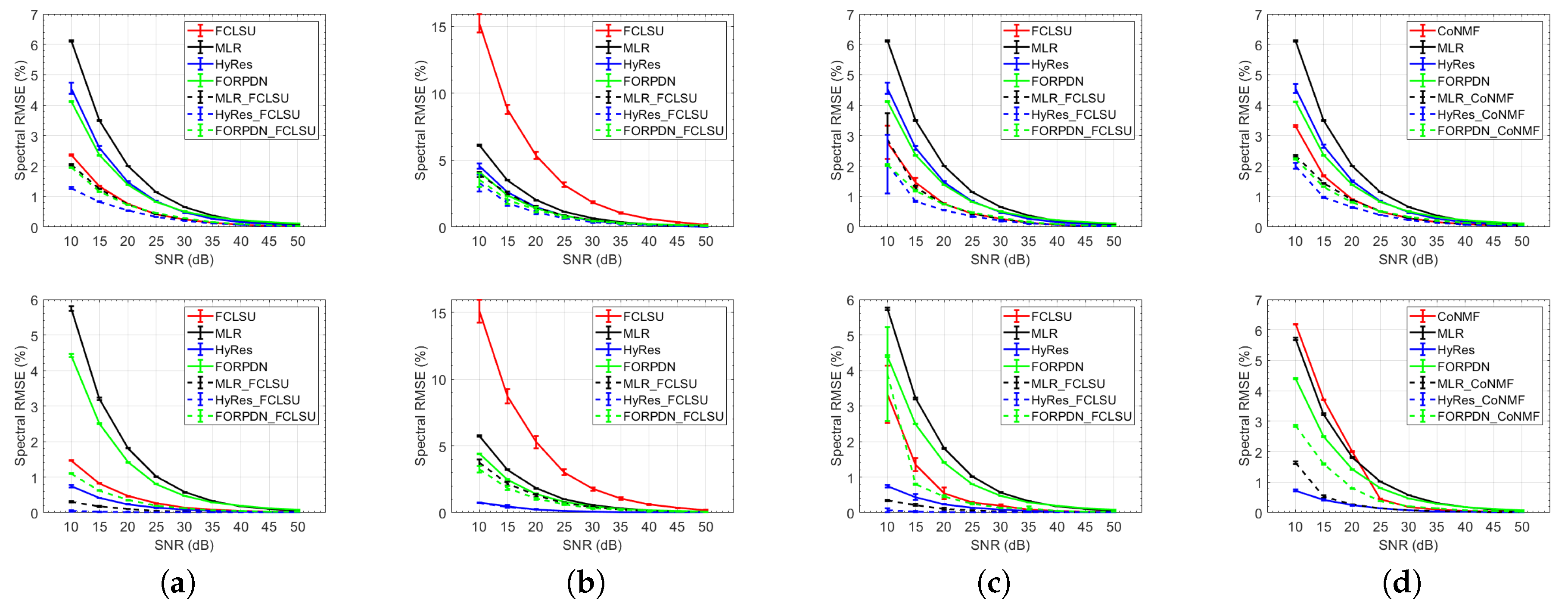
As discussed above, unmixing algorithms use a low-rank model for HSI (i.e., Model (2)), similar to low-rank denoising techniques. In this experiment, we evaluated the denoising performance of spectral unmixing. To do so, we reconstructed the image by using the estimated abundances () and compared it to the original noiseless image in terms of the spectral RMSE. This performance was then compared to the performance of the denoising techniques MLR, HyRes, and FORPDN. Additionally, we compared with the results, obtained by combining a denoising technique with spectral unmixing.
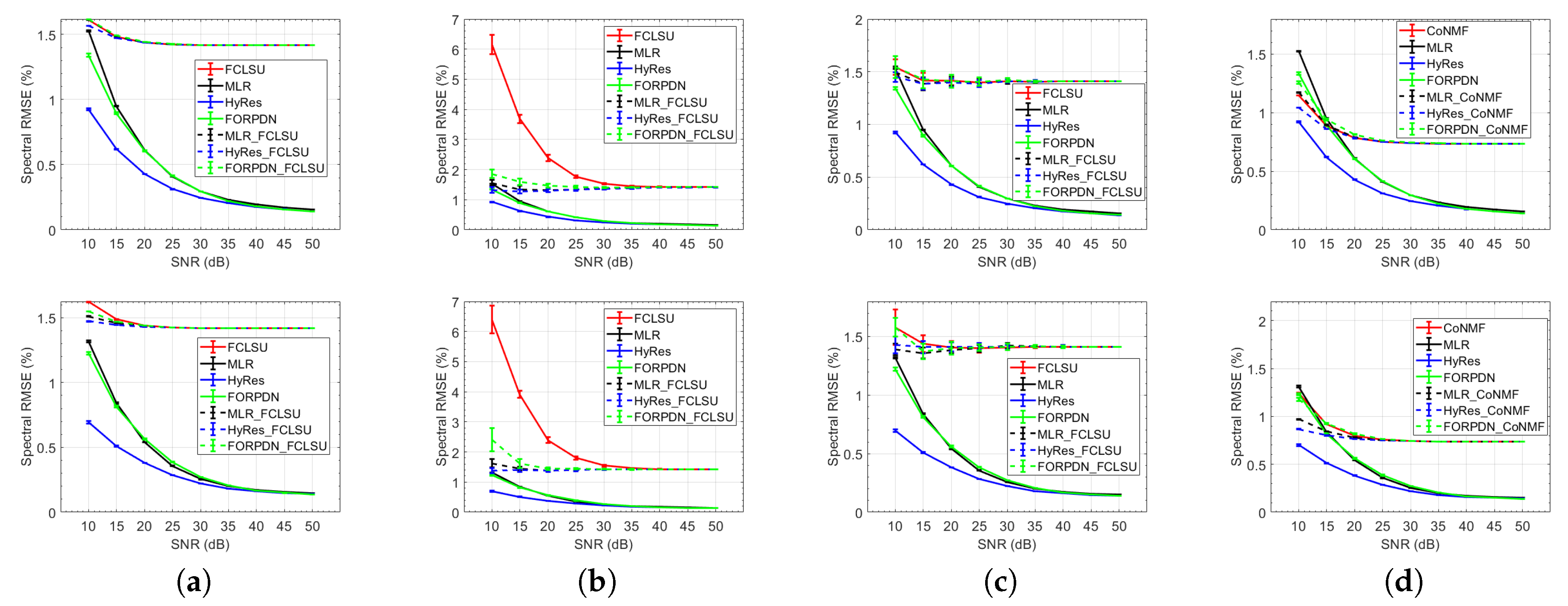
All results are shown in Figure 6 in terms of the spectral RMSE. Similar to the previous experiments, the four endmember scenarios were considered. The outcomes of this experiment could be summarized as follows:
- When comparing the solid lines, it could be observed that spectral unmixing was comparable to, or outperformed, the denoising techniques in all scenarios, except in the case of extracted endmembers. This could be attributed to the low-rank modeling ability of the unmixing.
- The more prior knowledge on the endmembers was provided, the better the denoising performance of the spectral unmixing. The best performance was obtained in Scenario (a), where the ground truth endmembers were given, and in Scenario (c), where a library of noise-free endmembers was provided. In Scenario (d), where CoNMF estimated smooth endmembers, the performance was good in the case of white noise, but became worse in the case of colored noise, where the middle bands were highly corrupted by noise. In Scenario (b), the extracted endmembers were noisy, which heavily deteriorated the denoising performance of the unmixing.
- In the case of colored noise, HyRes outperformed the other denoisers, as well as spectral unmixing. This again proved the superiority of this well-established low-rank denoising technique.
- When first denoising the images before unmixing, results generally improved over plain unmixing. Scenario (b) provided the lowest performance. The best results were obtained by the combination of HyRes and spectral unmixing. In the case of colored noise, the performance of HyRes was even further improved by spectral unmixing in Scenarios (a) and (c), but was not further improved by unmixing in Scenarios (b) and (d). This showed that the availability of prior knowledge on the endmembers, as in Scenarios (a) and (c), could further improve the denoising performance of a denoiser.
6. Real Dataset Experiments: The Samson Image
6.1. Denoising as Preprocessing for Unmixing
We should note that a prerequisite for validating the results in real images is the availability of ground truth endmembers and abundances and noise-free images. However, in real experiments, there always exists noise in the data, and the abundances are unknown.
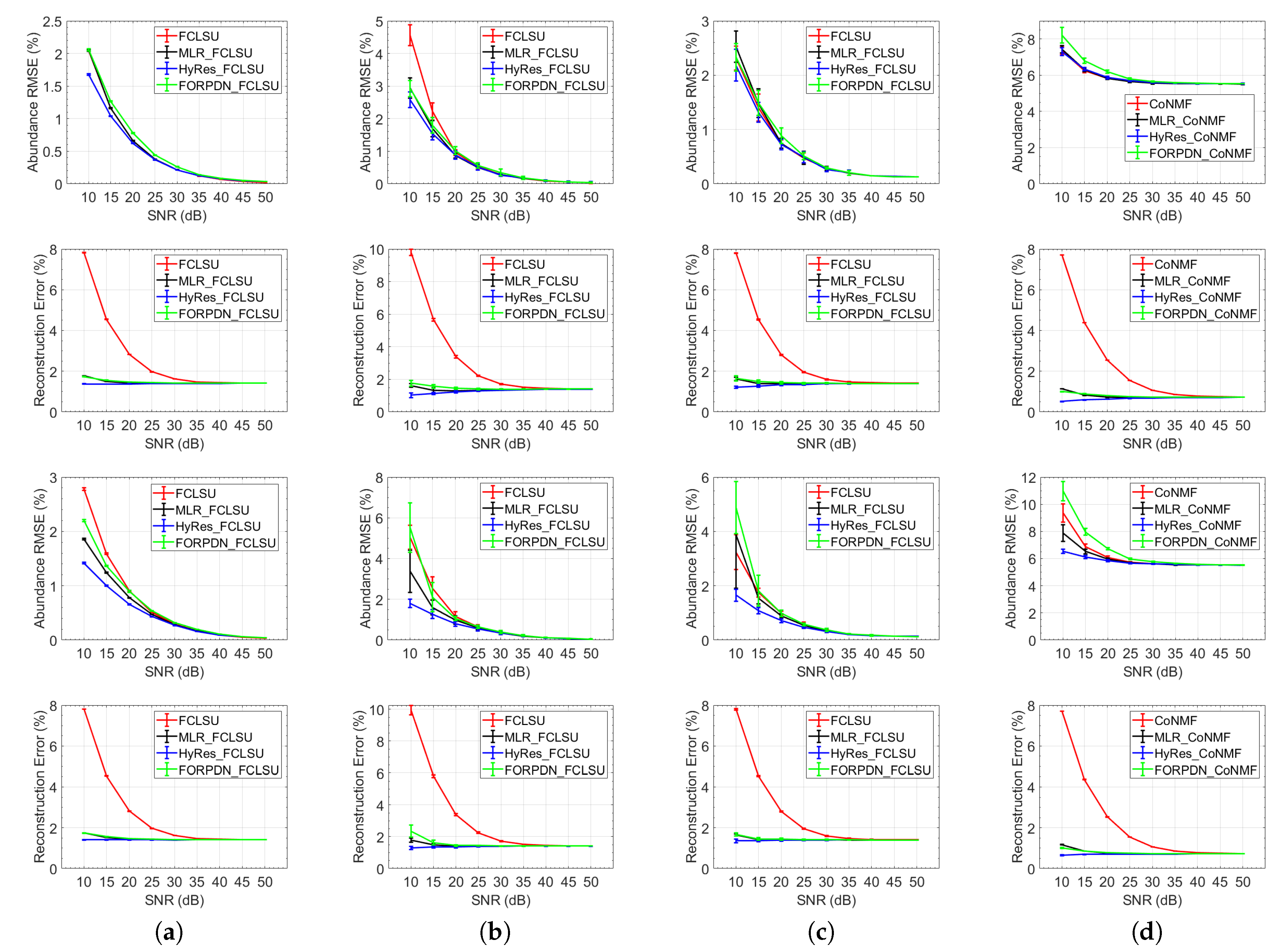
Figure 7 shows the performance of the spectral unmixing of noisy images and denoised images prior to unmixing, in the case of a real image, i.e., the Samson image. The outcome of the experiments could be summarized as follows:
- Similar to the simulated data, the reconstruction errors were high when unmixing noisy images, but drastically improved when performing denoising prior to spectral unmixing. A clear difference with the simulated image was that, even for very high SNR (50 dB), the reconstruction error was not zero. This could be attributed to the fact that the true endmembers were not known. As a consequence, a number of spectra fell outside of the simplex formed by the endmembers, which made a perfect reconstruction impossible.
- The abundance estimation did not improve proportionally. This confirmed that the spectral unmixing performance was not much affected by the noise even though large reconstruction errors were obtained.
- For Scenario (d), the abundance RMSE was about 5% higher than for the other scenarios, even for very high SNR. This phenomenon coincided with a lower reconstruction error than in the other scenarios. This could be attributed to the fact that the objective function of CoNMF entailed the minimization of the reconstruction error. Since the estimated endmembers did not necessarily correspond to the true endmembers, this came with a cost of poor abundance estimation.
- The effect of denoising on the abundance estimation was less pronounced than in the simulated case. In case of white noise, only in the scenario of extracted endmembers, a clear improvement could be observed when the noisy image was denoised prior to unmixing, particularly for low SNR. In Scenario (a), only HyRes could slightly improve the results; in Scenarios (c) and (d), denoising did not improve the abundance estimation.
- In the case of colored noise, the use of HyRes as preprocessing clearly improved the abundance estimation in all four scenarios, which once again confirmed the advantage of the using a well-established low-rank denoiser as preprocessing for unmixing.
6.2. Unmixing as a Denoiser
Figure 8 shows the Spectral RMSE for the Samson dataset, after denoising and after unmixing and reconstructing the image, with and without prior denoising. The following observations could be made:
- The results were quite different from the simulation results. In all scenarios, although the denoising performance of spectral unmixing was not bad at all, it was considerably lower than that of the denoising techniques.
- Even for very high SNR, the spectral RMSE after unmixing was not zero. This could partially be attributed to the same problem as with the reconstruction errors. The endmembers were not the true ones, leading to a reconstructed image that deviated from the observed image. In Scenario (b), this effect became more prominent for lower SNR, as the noise prevented extracting correct endmembers. In Scenario (d), the effect was smaller, since CoNMF estimated the endmembers by reducing the reconstruction error.
- One other possible reason of the large difference in denoising behavior between the real and simulated cases was that the real data did not exactly follow the linear model, e.g., due to nonlinearities and other nuisances, caused, e.g., by scattered light. This caused the endmembers and the abundance estimates to be incorrect. As a result, in real images, the reconstructed image after unmixing differed from the original image, already in noiseless situations (high SNR). Therefore, in real images, unmixing was not a good denoiser, compared to the denoising techniques. In the simulated image, linear data were simulated and therefore fit the model perfectly.
- Prior denoising before spectral unmixing did not improve the results. In Scenario (d), it even slightly deteriorated the results. Only in Scenario (b), the results were improved in the case of a low SNR, because the denoising reduced the chances to extract wrong endmembers.
- The denoising techniques themselves had a small nonzero spectral RMSE in the case of high SNR. This could be attributed to the fact that the Samson image in itself contained some small amounts of real noise.
- In the case of colored noise, the denoising techniques tended to perform slightly better and the unmixing slightly worse when compared to the white noise situation. Of the denoising techniques, HyRes performed the best.
Finally, all the experiments were also performed on the Jasper Ridge image. The results were very similar to the ones obtained on the Samson image, and therefore, they are not presented in this paper.
7. Discussion
The combination of unmixing and denoising has been treated in some recent studies. Several research works [35,39,40] developed specific methods that could cope with noise and perform denoising and unmixing simultaneously. In [32,33,34], it was shown that denoising may help to boost the endmember extraction and the unmixing performance. On the other hand, it was observed that spectral unmixing had denoising performance, in particular when employing low-noise endmembers, obtained by prior knowledge in the form of class information [36] or library endmembers [38].
In this paper, the goal was to conduct a comprehensive study on the topic to verify the findings of the literature and to draw more general conclusions, by studying (1) different noise situations, i.e., white and colored noise with a broad range of SNR values, (2) different unmixing strategies, i.e., four different ways of obtaining endmembers, and (3) different denoising strategies, i.e., three different types of denoising techniques. We studied the use of denoising to boost the unmixing performance and the performance of unmixing as a denoiser on one simulated and two real HSI datasets.
From the experiments, it could be concluded that noise played a crucial role when it came to spectral unmixing of HSIs. As a major conclusion, we could state that spectral unmixing was resilient to the effects of noise, in the sense that it could obtain reasonable abundances, despite a very high reconstruction error, and that it generated reconstructed images in which most of the noise was removed. When applied as a denoiser, the resilience of spectral unmixing to noise became clear. This could be attributed to the fact that spectral unmixing was a low-rank modeling technique, similar to many low-rank denoising methods that are known to be superior denoising techniques. In real datasets, the performance of unmixing as a denoiser was lower compared to state-of-the-art denoising techniques. We believe that this is because real datasets do not exactly follow the linear model, due to nonlinearities and other nuisances, caused, e.g., by scattered light. This caused the applied endmembers and the abundance estimates to be incorrect.
Prior denoising of images before performing the spectral unmixing had positive effects on both the unmixing and denoising performances of the spectral unmixing. The effect of prior denoising was more substantial when the image contained high levels of noise. In general, colored noise had more effect on the unmixing and denoising performances of the unmixing techniques than white noise. In that case, the effect of prior denoising was more prominent.
Another major conclusion was that the way the endmembers were treated had a major impact on the results. The best unmixing results were obtained when endmembers were noise-free. These could be ground truth endmembers Scenario (a)) or endmembers from libraries (Scenario (c)). If endmembers needed to be extracted from the noisy image (Scenario (b)), the results were the poorest, and prior denoising had the highest effect. When endmembers were estimated along with the abundances (Scenario (d)), with the purpose of optimizing the reconstruction error, this came at the cost of poor abundance estimation. Apart from the effects of noisy endmembers, the noise also caused the application of incorrect endmembers. Noise in images may cause an extraction of incorrect endmembers, a matching of extracted endmembers to incorrect library endmembers, or an estimation of incorrect endmembers. As a consequence, a large proportion of spectra fell outside the simplex spanned by these endmembers, leading to incorrect spectral unmixing results.
The Effect of Noise and Denoising on Endmember Estimation/Extraction
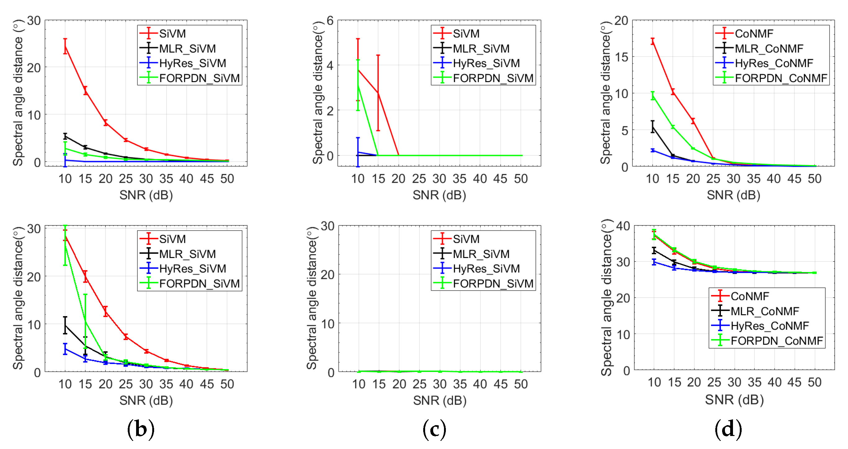
On the one hand, as we showed above, the quality of the estimated or extracted endmembers considerably affected the final abundance estimation and the spectral RMSE. On the other hand, denoising could degrade the spectral information and destroy the shape of the endmembers. Therefore, it was of interest to evaluate the quality of the estimated/extracted endmembers in noisy situations and after denoising. In this subsection, we further discuss the results of the conducted experiments, however from the point of view of the extracted/estimated endmembers. To evaluate the effect of noise and the denoising algorithms on the extracted/estimated endmembers, we measured the spectral angle distance (SAD) in degrees, defined by:
where is the ground truth endmember and is the estimated/extracted one. Figure 9 shows the SAD of the obtained endmembers for the Scenarios (b–d) (in Scenario (a), the ground truth endmembers were applied) as a function of SNR, without and with prior denoising, in the simulated and Samson dataset. Only the colored noise case () is shown. For white noise, similar results were observed.
The results on the simulated and the real dataset showed similar trends. The results strongly coincided with the results of the abundance estimation. When the endmembers needed to be extracted from the noisy data (Scenario (b)), the endmember quality was considerably affected by the noise and improved after prior denoising. Since in Scenario (c), the extracted endmembers were matched to noise-free library endmembers, the obtained SAD were very low. Only when SNR was lower than 20 dB in the simulated dataset, a deviation became visible, because then, the results were matched to the wrong endmember. In that case, prior denoising improved the endmember quality and consequently the abundance estimation performance. In case endmembers were estimated along with the fractional abundances using CoNMF (Scenario (d)), the noise affected the endmember quality, and prior denoising improved the results, in particular for SNR lower than 30 dB. In the real dataset, a bias in the SAD was observed, similar to what was observed in the abundance errors. This could again be attributed to the fact that a real dataset does not perfectly follow the linear model, and linear unmixing generates reconstruction errors, even in noise-free situations. Since CoNMF was forced to minimize the reconstruction error, it would estimate endmembers that deviated from the actual ones.
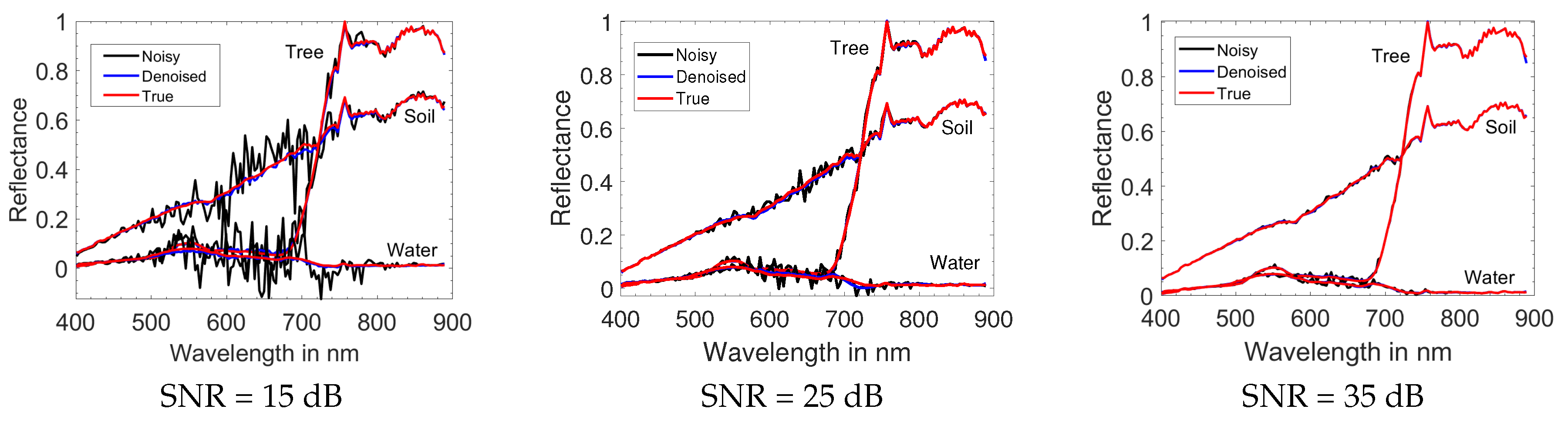
Although overall, the obtained SAD values were low, the shape of the endmember spectra may be significantly distorted. To evaluate this, Figure 10 compares the endmembers extracted by SiVM to the ground truth endmembers of the Samson image, for three different noise levels, i.e., SNR = 15, 25, and 35 dB, without and with pre-denoising. Similar trends were observed for other values of the SNR. For a better visual representation, only the results of the most effective denoising technique used in the experiments (i.e., HyRes) are shown. As can be observed, SiVM extracted relevant endmembers, even in noisy situations. After denoising the image, the extracted endmembers were very close to the true ones, and no significant distortion of the endmember spectra could be observed.
Finally, we want to stress that high quality ground truth data for spectral unmixing are hard to obtain, which makes it hard to validate the performance of spectral unmixing experiments on real data.
8. Conclusions
In this paper, we investigated the influence of noise on spectral unmixing of hyperspectral images (HSIs). In particular, we studied the denoising performance of HSI unmixing techniques and the effects of HSI denoising prior to HSI unmixing. Four different unmixing scenarios were studied based on the availability of endmembers: the use of ground truth endmembers, the blind extraction of endmembers, the use of library endmembers, and the estimation of endmembers along with the fractional abundances. As an unmixing method, FCLSU was applied, except for the last scenario, for which CoNMF was applied. Three denoising techniques were selected for the experiments: HyRes, a low-rank model-based technique, FORPDN, a full-rank model-based technique, and MLR, a conventional method based on multiple regression.
The experiments were carried out on one simulated dataset and two real HSIs. The study comprised white, as well as colored noise with a broad range of SNR values. From the experiments, we drew the following main conclusions:
- Spectral unmixing was highly resilient to noise, allowing it to adequately estimate fractional abundances in noisy images and producing reconstructed images with good denoising performance.
- A crucial role was played by the way endmembers were provided. The more prior knowledge about the endmembers was available, the better the unmixing and denoising performance of an unmixing procedure.
- Prior denoising could boost the unmixing, as well as the denoising performance of an unmixing procedure. This became more prominent in high noise and colored noise situations, when less prior knowledge of the endmembers was available or when incorrect endmembers were applied. To validate these findings in real datasets, accurate endmember and fractional abundance ground truth information was invaluable.
Author Contributions
B.R. wrote the original draft with a considerable contribution from B.K. They also performed the experiments and prepared the results. The two first authors had an equal contribution. P.S. significantly improved the manuscript both technically and grammatically, besides improving its presentation. P.G. revised the manuscript. All authors have read and agreed to the published version of the manuscript.
Funding
This research was funded by the Alexander von Humboldt foundation and BELSPO (Belgian Science Policy Office) in the frame of the STEREO III program, Project GEOMIX (SR/06/357).
Conflicts of Interest
The authors declare no conflict of interest.
References
- Ghamisi, P.; Yokoya, N.; Li, J.; Liao, W.; Liu, S.; Plaza, J.; Rasti, B.; Plaza, A. Advances in Hyperspectral Image and Signal Processing: A Comprehensive Overview of the State of the Art. IEEE Geosci. Remote. Sens. Mag. 2017, 5, 37–78. [Google Scholar] [CrossRef] [Green Version]
- Parente, M.; Plaza, A. Survey of geometric and statistical unmixing algorithms for hyperspectral images. In Proceedings of the 2nd Workshop on Hyperspectral Image and Signal Processing: Evolution in Remote Sensing, Reykjavik, Iceland, 14–16 June 2010; pp. 1–4. [Google Scholar]
- Miao, L.; Qi, H. Endmember Extraction From Highly Mixed Data Using Minimum Volume Constrained Nonnegative Matrix Factorization. IEEE Trans. Geosci. Remote. Sens. 2007, 45, 765–777. [Google Scholar] [CrossRef]
- Li, J.; Bioucas-Dias, J.M. Minimum Volume Simplex Analysis: A Fast Algorithm to Unmix Hyperspectral Data. In Proceedings of the IEEE International Geoscience and Remote Sensing Symposium (IGARSS), Boston, MA, USA, 7–11 July 2008; Volume 3, pp. 250–253. [Google Scholar]
- Chan, T.; Chi, C.; Huang, Y.; Ma, W. Convex analysis based minimum-volume enclosing simplex algorithm for hyperspectral unmixing. In Proceedings of the IEEE International Conference on Acoustics, Speech and Signal Processing, Taipei, Taiwan, 19–24 April 2009; pp. 1089–1092. [Google Scholar]
- Li, J.; Bioucas-Dias, J.M.; Plaza, A. Collaborative nonnegative matrix factorization for remotely sensed hyperspectral unmixing. In Proceedings of the IEEE International Geoscience and Remote Sensing Symposium (IGARSS), Munich, Germany, 22–27 July 2012; pp. 3078–3081. [Google Scholar]
- Iordache, M.; Bioucas-Dias, J.M.; Plaza, A. Sparse Unmixing of Hyperspectral Data. IEEE Trans. Geosci. Remote. Sens. 2011, 49, 2014–2039. [Google Scholar] [CrossRef] [Green Version]
- Iordache, M.; Bioucas-Dias, J.M.; Plaza, A. Total Variation Spatial Regularization for Sparse Hyperspectral Unmixing. IEEE Trans. Geosci. Remote. Sens. 2012, 50, 4484–4502. [Google Scholar] [CrossRef] [Green Version]
- Iordache, M.; Bioucas-Dias, J.M.; Plaza, A. Collaborative Sparse Regression for Hyperspectral Unmixing. IEEE Trans. Geosci. Remote. Sens. 2014, 52, 341–354. [Google Scholar] [CrossRef] [Green Version]
- Boardman, J.W. Geometric mixture analysis of imaging spectrometry data. In Proceedings of the IEEE International Geoscience and Remote Sensing Symposium (IGARSS), Pasadena, CA, USA, 8–12 August 1994; Volume 4, pp. 2369–2371. [Google Scholar]
- Heinz, D.C.; Chein-I-Chang. Fully constrained least squares linear spectral mixture analysis method for material quantification in hyperspectral imagery. IEEE Trans. Geosci. Remote. Sens. 2001, 39, 529–545. [Google Scholar] [CrossRef] [Green Version]
- Rasti, B.; Scheunders, P.; Ghamisi, P.; Licciardi, G.; Chanussot, J. Noise Reduction in Hyperspectral Imagery: Overview and Application. Remote. Sens. 2018, 10, 482. [Google Scholar] [CrossRef] [Green Version]
- Atkinson, I.; Kamalabadi, F.; Jones, D. Wavelet-based hyperspectral image estimation. In Proceedings of the IEEE International Geoscience and Remote Sensing Symposium (IGARSS), Toulouse, France, 21–25 July 2003; Volume 2, pp. 743–745. [Google Scholar]
- Qian, Y.; Ye, M. Hyperspectral Imagery Restoration Using Nonlocal Spectral-Spatial Structured Sparse Representation With Noise Estimation. IEEE J. Sel. Top. Appl. Earth Obs. Remote. Sens. 2013, 6, 499–515. [Google Scholar] [CrossRef]
- Rasti, B.; Sveinsson, J.R.; Ulfarsson, M.O.; Benediktsson, J.A. Hyperspectral image denoising using 3D wavelets. In Proceedings of the IEEE International Geoscience and Remote Sensing Symposium (IGARSS), Munich, Germany, 22–27 July 2012; pp. 1349–1352. [Google Scholar]
- Rasti, B.; Sveinsson, J.R.; Ulfarsson, M.O.; Benediktsson, J.A. Hyperspectral Image Denoising Using First Order Spectral Roughness Penalty in Wavelet Domain. IEEE J. Sel. Top. Appl. Earth Obs. Remote. Sens. 2014, 7, 2458–2467. [Google Scholar] [CrossRef]
- Rasti, B.; Sveinsson, J.R.; Ulfarsson, M.O.; Benediktsson, J.A. Wavelet based hyperspectral image restoration using spatial and spectral penalties. In Image and Signal Processing for Remote Sensing XIX; International Society for Optics and Photonics: Bellingham, WA, USA, 2013; Volume 8892, p. 88920I. [Google Scholar]
- Chen, S.L.; Hu, X.Y.; Peng, S.L. Hyperspectral Imagery Denoising Using a Spatial-Spectral Domain Mixing Prior. J. Comput. Sci. Technol. 2012, 27, 851–861. [Google Scholar] [CrossRef]
- Yuan, Q.; Zhang, L.; Shen, H. Hyperspectral Image Denoising Employing a Spectral-Spatial Adaptive Total Variation Model. IEEE Trans. Geosci. Remote. Sens. 2012, 50, 3660–3677. [Google Scholar] [CrossRef]
- Rasti, B.; Ulfarsson, M.; Sveinsson, J. Hyperspectral Subspace Identification Using SURE. IEEE Geosci. Remote. Sens. Lett. 2015, 12, 2481–2485. [Google Scholar] [CrossRef]
- Bioucas-Dias, J.; Nascimento, J. Hyperspectral Subspace Identification. IEEE Trans. Geosci. Remote. Sens. 2008, 46, 2435–2445. [Google Scholar] [CrossRef] [Green Version]
- Liu, X.; Bourennane, S.; Fossati, C. Denoising of Hyperspectral Images Using the PARAFAC Model and Statistical Performance Analysis. IEEE Trans. Geosci. Remote. Sens. 2012, 50, 3717–3724. [Google Scholar] [CrossRef]
- Rasti, B.; Sveinsson, J.R.; Ulfarsson, M.O.; Benediktsson, J.A. Hyperspectral image restoration using wavelets. In Image and Signal Processing for Remote Sensing XIX; International Society for Optics and Photonics: Bellingham, WA, USA, 2013; Volume 8892, p. 889207. [Google Scholar]
- Rasti, B. Sparse Hyperspectral Image Modeling and Restoration. Ph.D. Thesis, University of Iceland, Reykjavík, Iceland, 2014. [Google Scholar]
- Rasti, B.; Sveinsson, J.; Ulfarsson, M. Wavelet-Based Sparse Reduced-Rank Regression for Hyperspectral Image Restoration. IEEE Trans. Geosci. Remote. Sens. 2014, 52, 6688–6698. [Google Scholar] [CrossRef]
- Rasti, B.; Sveinsson, J.R.; Ulfarsson, M.O. Total Variation Based Hyperspectral Feature Extraction. In Proceedings of the IEEE International Geoscience and Remote Sensing Symposium (IGARSS), Quebec City, QC, Canada, 13–18 July 2014; pp. 4644–4647. [Google Scholar]
- Rasti, B.; Ulfarsson, M.O.; Ghamisi, P. Automatic Hyperspectral Image Restoration Using Sparse and Low-Rank Modeling. IEEE Geosci. Remote. Sens. Lett. 2017, 14, 2335–2339. [Google Scholar] [CrossRef] [Green Version]
- Liu, X.; Bourennane, S.; Fossati, C. Reduction of Signal-Dependent Noise From Hyperspectral Images for Target Detection. IEEE Trans. Geosci. Remote. Sens. 2014, 52, 5396–5411. [Google Scholar]
- Sun, L.; Jeon, B.; Zheng, Y.; Wu, Z. Hyperspectral Image Restoration Using Low-Rank Representation on Spectral Difference Image. IEEE Geosci. Remote. Sens. Lett. 2017, 14, 1151–1155. [Google Scholar] [CrossRef]
- Zhang, H.; He, W.; Zhang, L.; Shen, H.; Yuan, Q. Hyperspectral Image Restoration Using Low-Rank Matrix Recovery. IEEE Trans. Geosci. Remote. Sens. 2014, 52, 4729–4743. [Google Scholar] [CrossRef]
- Rasti, B.; Ghamisi, P.; Benediktsson, J.A. Hyperspectral Mixed Gaussian and Sparse Noise Reduction. IEEE Geosci. Remote. Sens. Lett. 2020, 17, 474–478. [Google Scholar] [CrossRef]
- Kocakusaklar, B.; Kahraman, N. The Effect of Impulse Denoising on Geometric Based Hyperspectral Unmixing. Int. J. Nat. Sci. Res. 2016, 4, 83–91. [Google Scholar] [CrossRef] [Green Version]
- Swarna, M.; Sowmya, V.; Soman, K.P. Effect of Denoising on Dimensionally Reduced Sparse Hyperspectral Unmixing. Procedia Comput. Sci. 2017, 115, 391–398. [Google Scholar] [CrossRef]
- Qu, Y.; Qi, H. uDAS: An Untied Denoising Autoencoder With Sparsity for Spectral Unmixing. IEEE Trans. Geosci. Remote. Sens. 2019, 57, 1698–1712. [Google Scholar] [CrossRef]
- Aggarwal, H.K.; Majumdar, A. Hyperspectral Unmixing in the Presence of Mixed Noise Using Joint-Sparsity and Total Variation. IEEE J. Sel. Top. Appl. Earth Obs. Remote. Sens. 2016, 9, 4257–4266. [Google Scholar] [CrossRef]
- Cerra, D.; Müller, R.; Reinartz, P. Noise Reduction in Hyperspectral Images Through Spectral Unmixing. IEEE Geosci. Remote. Sens. Lett. 2014, 11, 109–113. [Google Scholar] [CrossRef] [Green Version]
- Ertürk, A. Enhanced Unmixing-Based Hyperspectral Image Denoising Using Spatial Preprocessing. IEEE J. Sel. Top. Appl. Earth Obs. Remote. Sens. 2015, 8, 2720–2727. [Google Scholar] [CrossRef]
- Ertürk, A. Sparse unmixing based denoising for hyperspectral images. In Proceedings of the IEEE International Geoscience and Remote Sensing Symposium (IGARSS), Beijing, China, 10–15 July 2016; pp. 7006–7009. [Google Scholar]
- Ince, T.; Dundar, T. Simultaneous Nonconvex Denoising and Unmixing for Hyperspectral Imaging. IEEE Access 2019, 7, 124426–124440. [Google Scholar] [CrossRef]
- Yang, J.; Zhao, Y.; Chan, J.C.; Kong, S.G. Coupled Sparse Denoising and Unmixing With Low-Rank Constraint for Hyperspectral Image. IEEE Trans. Geosci. Remote. Sens. 2016, 54, 1818–1833. [Google Scholar] [CrossRef]
- Rasti, B.; Hong, D.; Hang, R.; Ghamisi, P.; Kang, X.; Chanussot, J.; Benediktsson, J.A. Feature Extraction for Hyperspectral Imagery: The Evolution from Shallow to Deep (Overview and Toolbox). IEEE Geosci. Remote. Sens. Mag. 2019. [Google Scholar]
- Heylen, R.; Burazerovic, D.; Scheunders, P. Fully Constrained Least Squares Spectral Unmixing by Simplex Projection. IEEE Trans. Geosci. Remote. Sens. 2011, 49, 4112–4122. [Google Scholar] [CrossRef]
- Craig, M.D. Minimum-volume transforms for remotely sensed data. IEEE Trans. Geosci. Remote. Sens. 1994, 32, 542–552. [Google Scholar] [CrossRef]
- Stein, C.M. Estimation of the Mean of a Multivariate Normal Distribution. Ann. Stat. 1981, 9, 1135–1151. [Google Scholar] [CrossRef]
- Zhu, F.; Wang, Y.; Fan, B.; Xiang, S.; Meng, G.; Pan, C. Spectral unmixing via data-guided sparsity. IEEE Trans. Image Process. 2014, 23, 5412–5427. [Google Scholar] [CrossRef] [PubMed] [Green Version]
Figure 1.
Simulated image. (a): Endmembers; (b): abundance maps.

Figure 2.
Samson image. (a): True-color image (red: 571.01 nm, green: 539.53 nm, blue: 432.48 nm); (b): endmembers; (c): abundance maps.
Figure 2.
Samson image. (a): True-color image (red: 571.01 nm, green: 539.53 nm, blue: 432.48 nm); (b): endmembers; (c): abundance maps.

Figure 3.
Jasper Ridge image. (a): True-color image (red: 570.14 nm, green: 532.11 nm, blue: 427.53 nm); (b): endmembers; (c): abundance maps.
Figure 3.
Jasper Ridge image. (a): True-color image (red: 570.14 nm, green: 532.11 nm, blue: 427.53 nm); (b): endmembers; (c): abundance maps.

Figure 4.
The noise variance along the spectral bands at SNR = 25 dB.

Figure 5.
Simulated data (top two rows and bottom two rows ): The results of unmixing in terms of abundance RMSE and reconstruction error as a function of the noise level of the observed image (in SNR). (a) Ground truth endmembers; (b) extracted endmembers; (c) library endmembers; (d) estimated endmembers. FCLSU, fully constrained least squares unmixing; FORPDN, first order spectral roughness penalty denoising; CoNMF, collaborative nonnegative matrix factorization; HyRes, hyperspectral restoration.

Figure 6.
Simulated data (top row and bottom row ): The denoising performance of spectral unmixing compared with the denoising techniques. (a) Ground truth endmembers; (b) extracted endmembers; (c) library endmembers; (d) estimated endmembers.
Figure 6.
Simulated data (top row and bottom row ): The denoising performance of spectral unmixing compared with the denoising techniques. (a) Ground truth endmembers; (b) extracted endmembers; (c) library endmembers; (d) estimated endmembers.

Figure 7.
Real data (top two rows and bottom two rows ): The spectral unmixing results on the Samson image in terms of abundance RMSE and reconstruction error. (a) Ground truth endmembers; (b) extracted endmembers; (c) library endmembers; (d) estimated endmembers.
Figure 7.
Real data (top two rows and bottom two rows ): The spectral unmixing results on the Samson image in terms of abundance RMSE and reconstruction error. (a) Ground truth endmembers; (b) extracted endmembers; (c) library endmembers; (d) estimated endmembers.

Figure 8.
Real data (top row and bottom row ): The denoising performance on the Samson image in terms of Spectral RMSE. (a) Ground truth endmembers; (b) extracted endmembers; (c) library endmembers; (d) estimated endmembers.
Figure 8.
Real data (top row and bottom row ): The denoising performance on the Samson image in terms of Spectral RMSE. (a) Ground truth endmembers; (b) extracted endmembers; (c) library endmembers; (d) estimated endmembers.

Figure 9.
The quality of the estimated/extracted endmembers in terms of spectral angle distance (SAD) in degrees on the simulated data (top row) and Samson data (bottom row) for colored noise (): (b) extracted endmembers; (c) library endmembers; (d) estimated endmembers.
Figure 9.
The quality of the estimated/extracted endmembers in terms of spectral angle distance (SAD) in degrees on the simulated data (top row) and Samson data (bottom row) for colored noise (): (b) extracted endmembers; (c) library endmembers; (d) estimated endmembers.

Figure 10.
The ground truth endmembers and the endmembers extracted by the simplex volume maximization technique (SiVM), without and with prior denoising of the Samson image using HyRes, in the cases of colored noise ().
Figure 10.
The ground truth endmembers and the endmembers extracted by the simplex volume maximization technique (SiVM), without and with prior denoising of the Samson image using HyRes, in the cases of colored noise ().

© 2020 by the authors. Licensee MDPI, Basel, Switzerland. This article is an open access article distributed under the terms and conditions of the Creative Commons Attribution (CC BY) license (http://creativecommons.org/licenses/by/4.0/).
Share and Cite
MDPI and ACS Style
Rasti, B.; Koirala, B.; Scheunders, P.; Ghamisi, P. How Hyperspectral Image Unmixing and Denoising Can Boost Each Other. Remote Sens. 2020, 12, 1728. https://0-doi-org.brum.beds.ac.uk/10.3390/rs12111728
AMA Style
Rasti B, Koirala B, Scheunders P, Ghamisi P. How Hyperspectral Image Unmixing and Denoising Can Boost Each Other. Remote Sensing. 2020; 12(11):1728. https://0-doi-org.brum.beds.ac.uk/10.3390/rs12111728
Chicago/Turabian StyleRasti, Behnood, Bikram Koirala, Paul Scheunders, and Pedram Ghamisi. 2020. "How Hyperspectral Image Unmixing and Denoising Can Boost Each Other" Remote Sensing 12, no. 11: 1728. https://0-doi-org.brum.beds.ac.uk/10.3390/rs12111728
Note that from the first issue of 2016, this journal uses article numbers instead of page numbers. See further details here.