Novel Ensemble Approaches of Machine Learning Techniques in Modeling the Gully Erosion Susceptibility

 , ,
, ,  ,
,  and
and
Abstract
:1. Introduction
2. Material and Methods
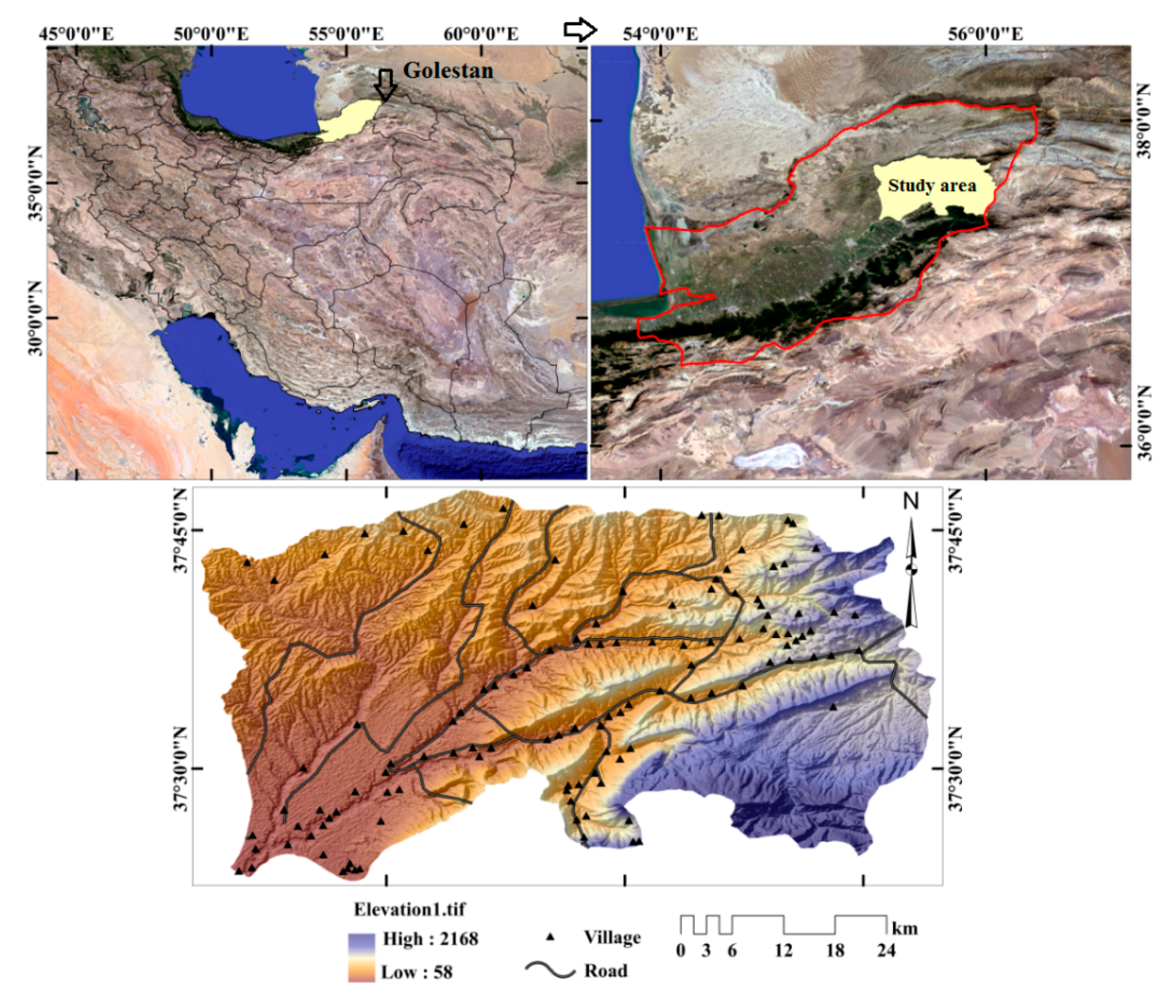
2.1. Study Area
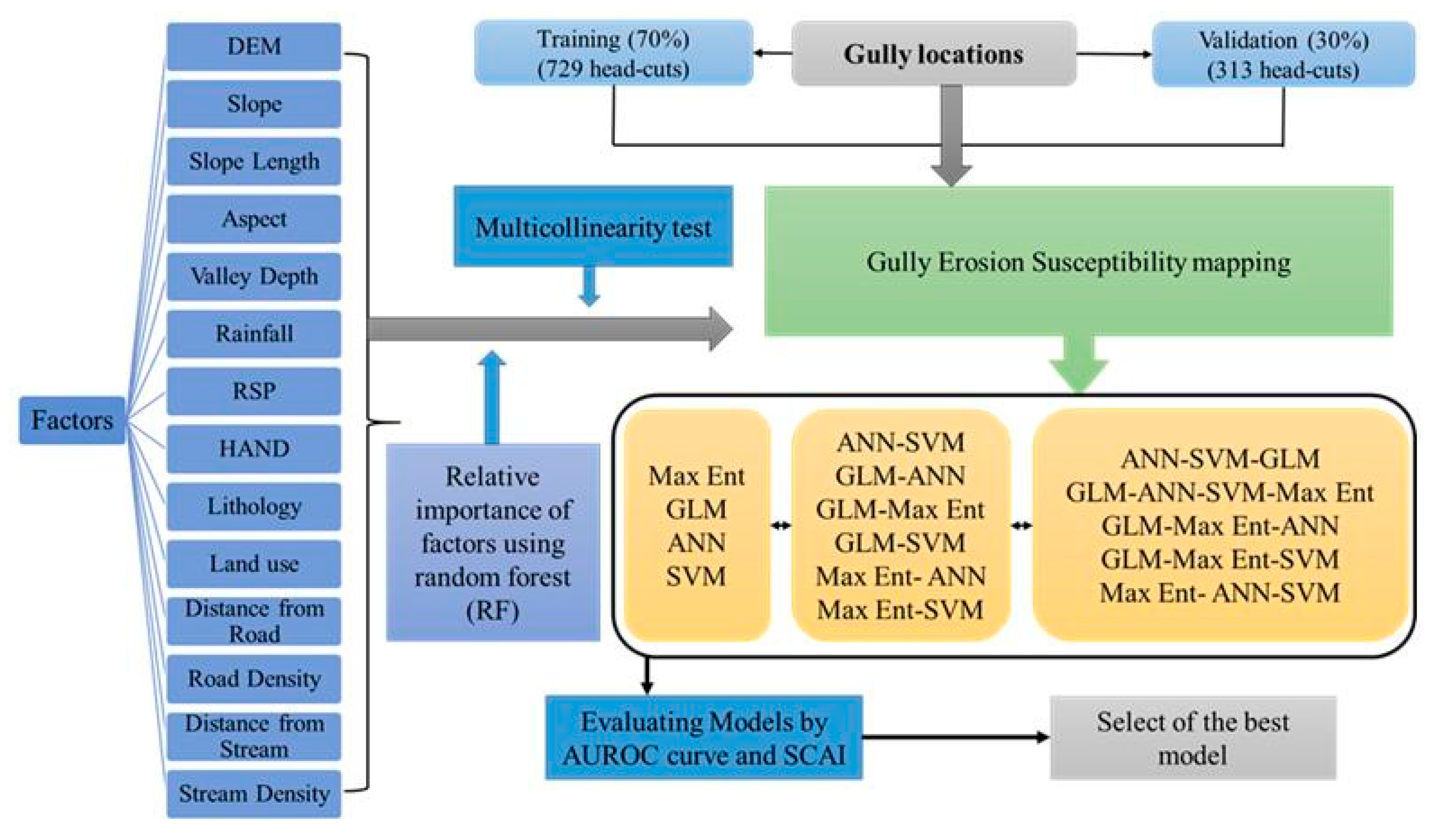
2.2. Methodology
- (i)
- To prepare the gully erosion inventory map and the GECFs dataset, 1042 gully head cut locations were identified using high-resolution images, field investigation, and global positioning system (GPS). Data for fourteen environmental factors identified from a literature review were compiled (data sources are described below).
- (ii)
- Multi-collinearity analysis among the GECFs using tolerance and variance inflation factor (VIF) techniques was done.
- (iii)
- The significance and effectiveness of GECFs was determined using the random forest (RF) model.
- (iv)
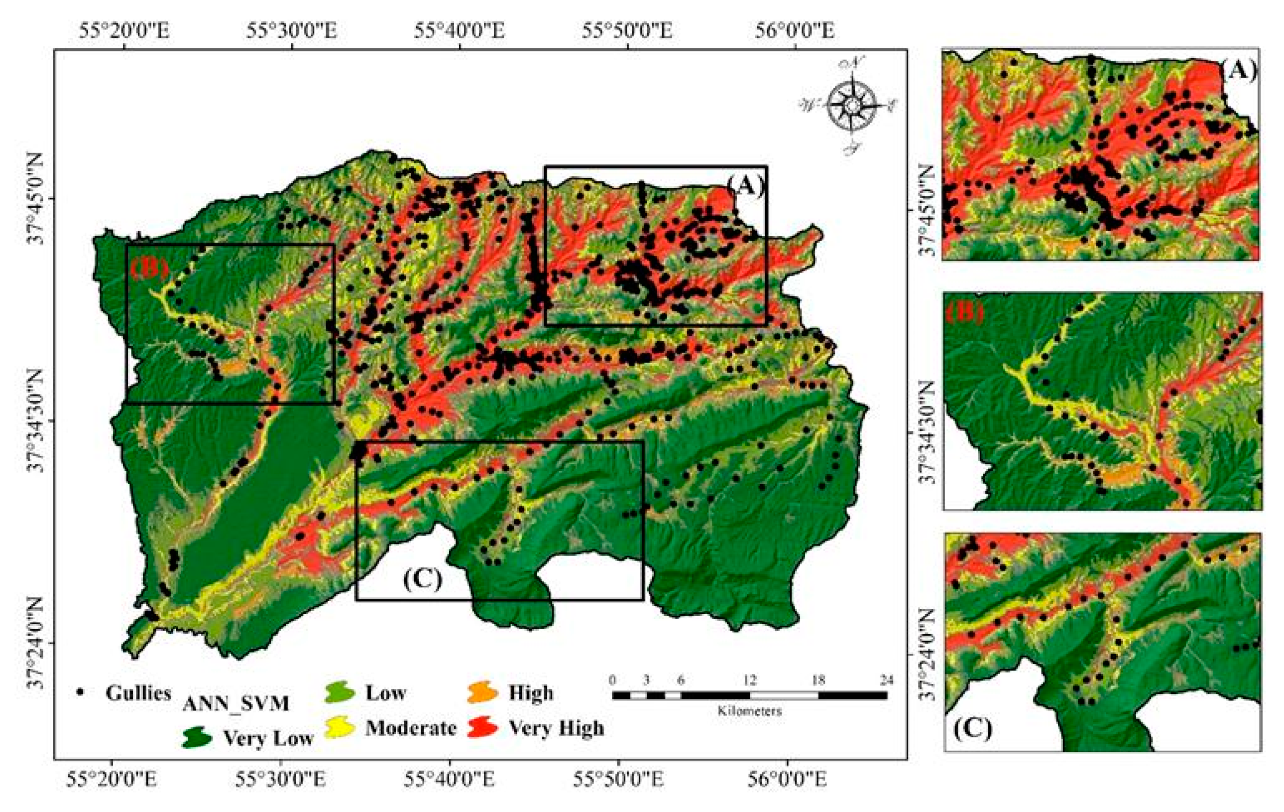
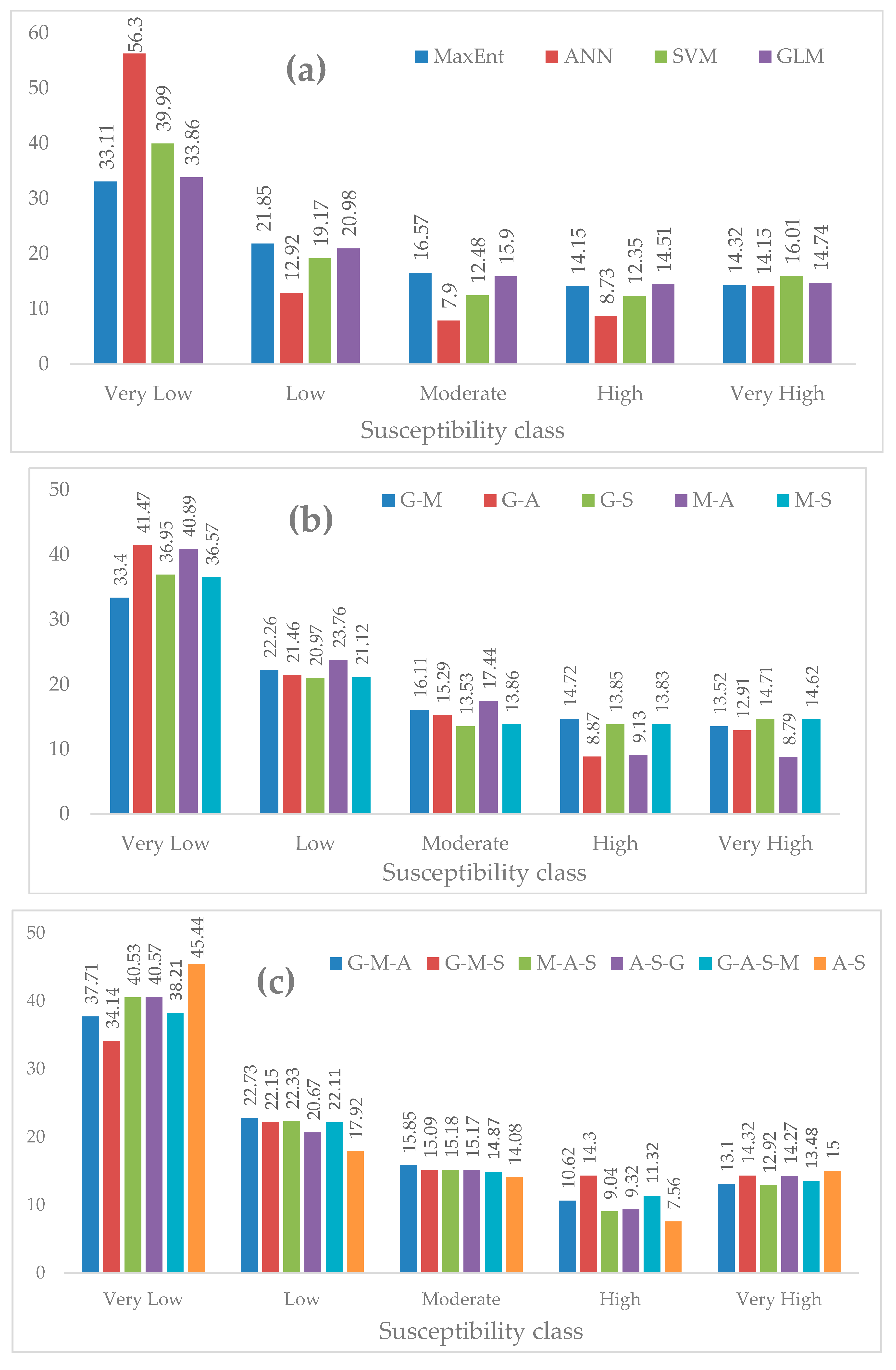
- GES maps were prepared with MaxEnt, ANN, SVM and GLM models. The ensemble models were prepared by combining sets of two, three and four models.
- (v)
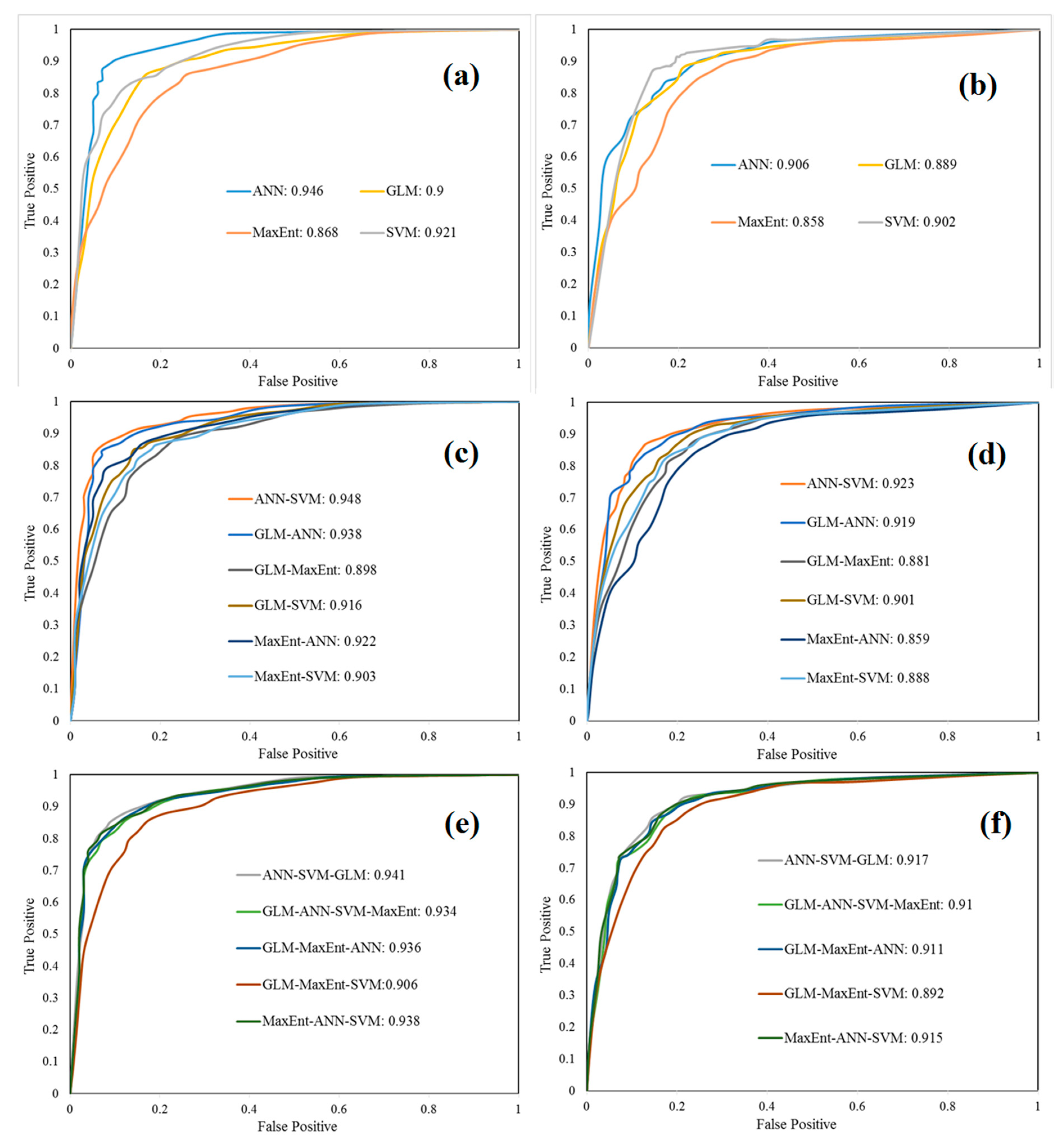
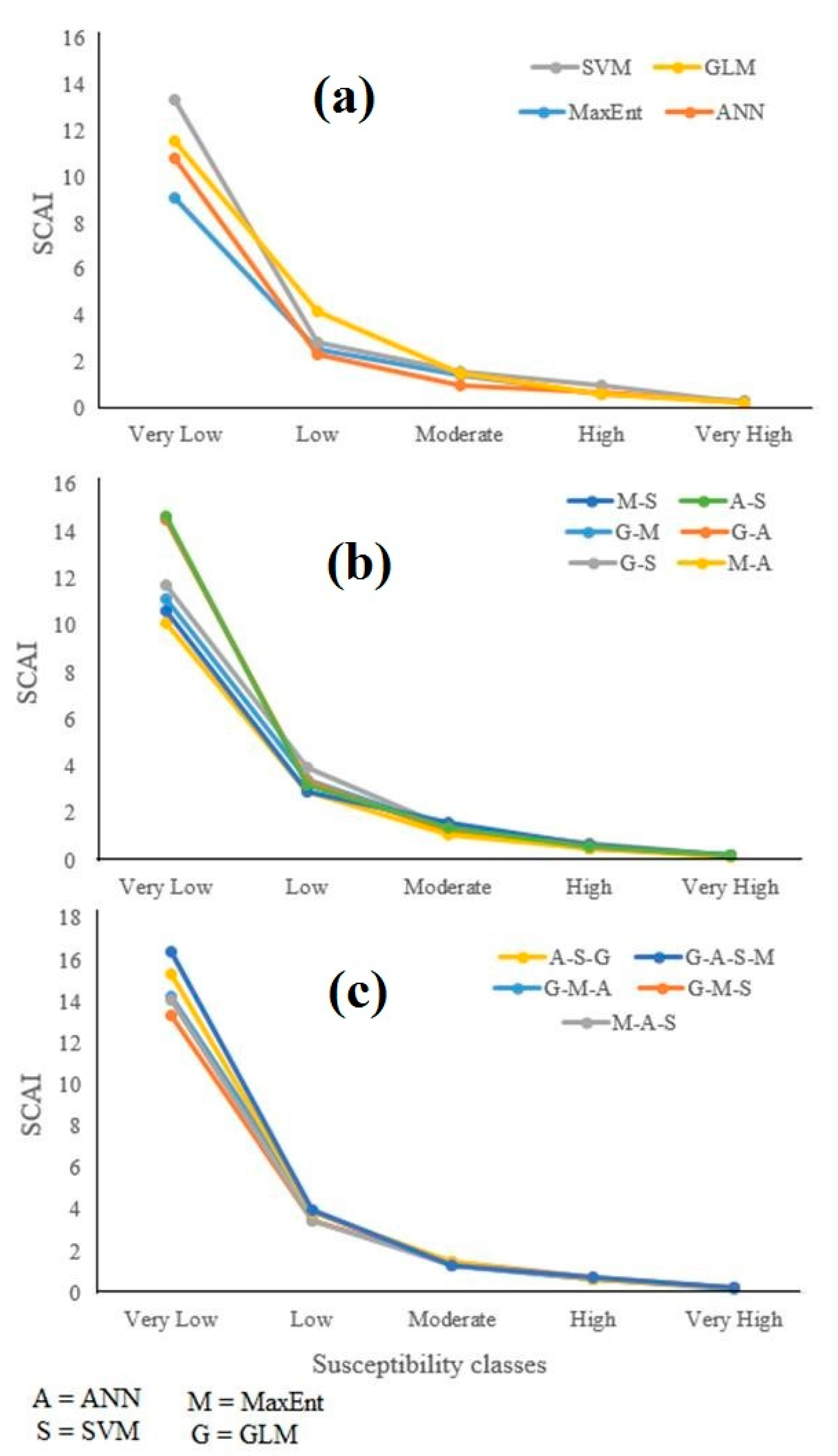
- The performances of gully erosion susceptibility models (GESMs) were validated with the area under receiver operating characteristic curve (AUROC) and seed cell area index (SCAI) methods.
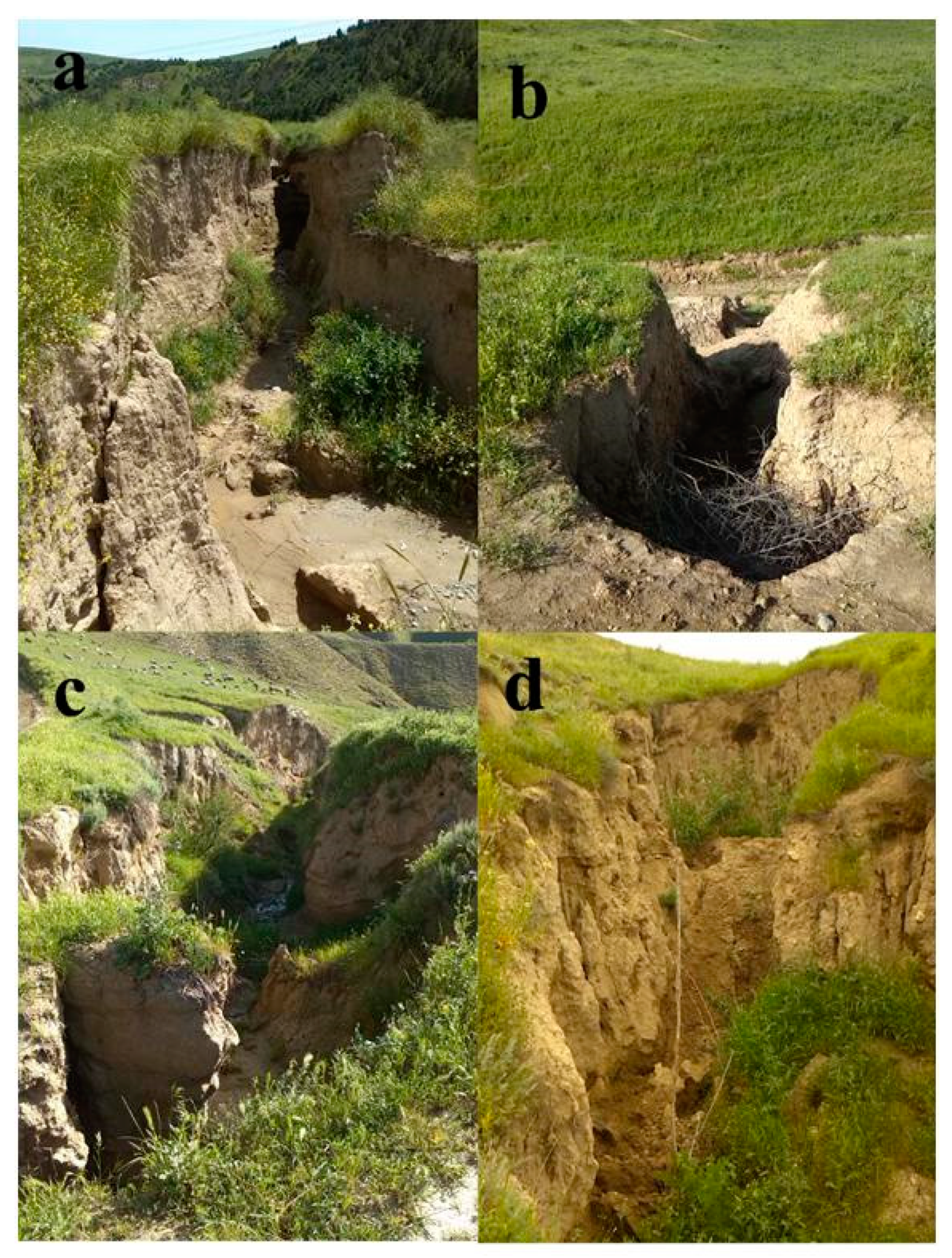
2.3. Gully Erosion Inventory Map (GEIM)
2.4. Preparing the Gully Erosion Conditioning Factors (GECFs)
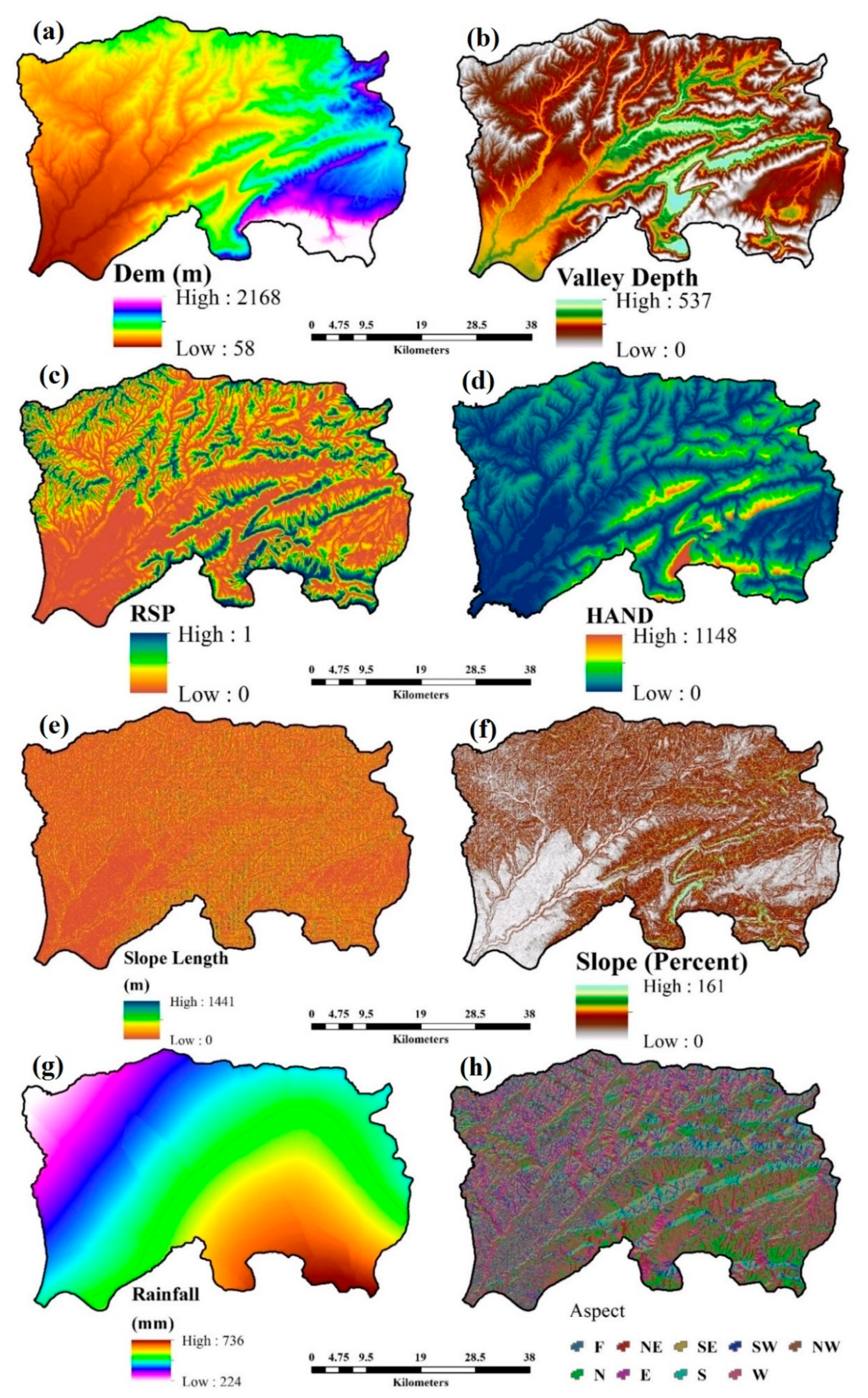
2.4.1. DEM Derived Factors
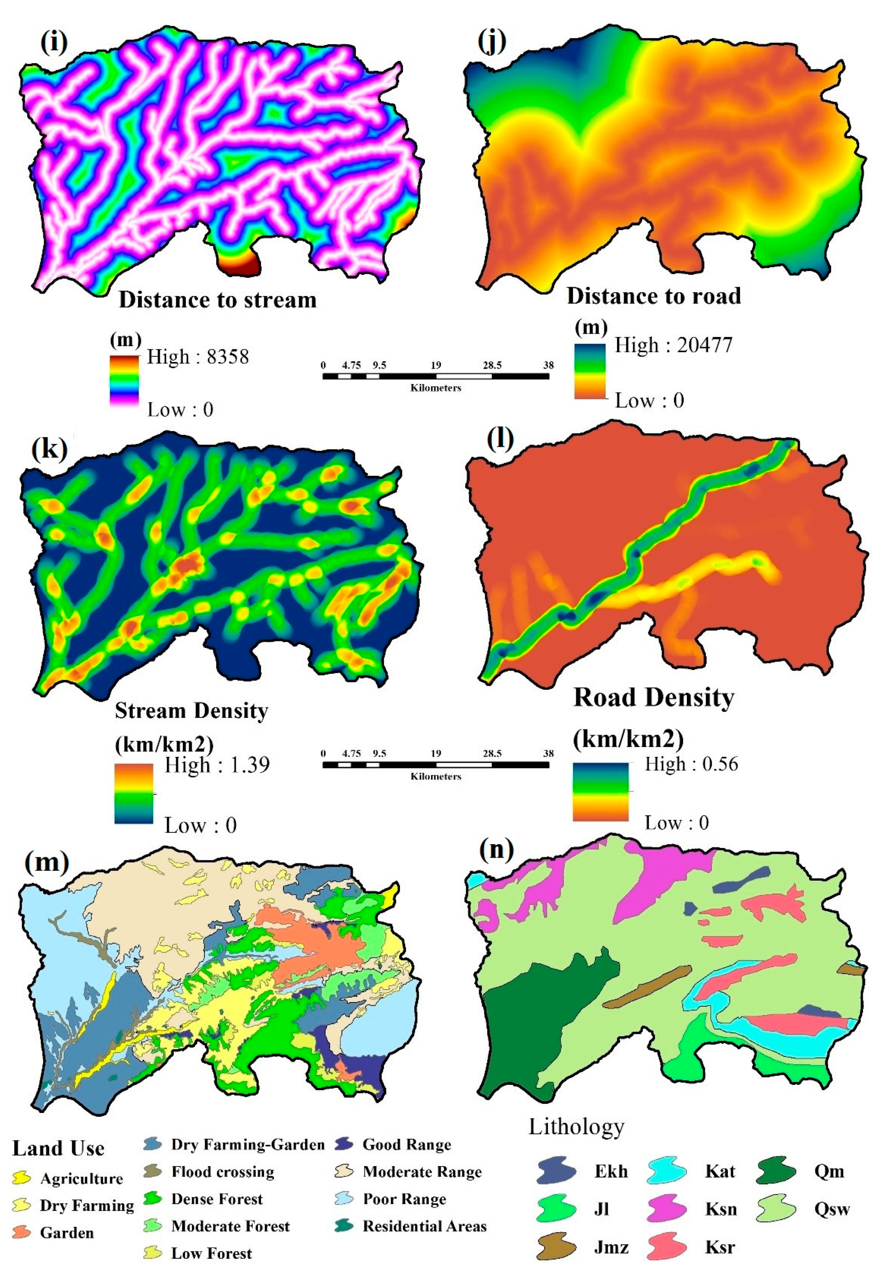
2.4.2. Hydrological Factors
2.4.3. Environmental Factors
2.5. Multi Collinearity Analysis
2.6. Methods
2.6.1. Maximum Entropy (MaxEnt)
2.6.2. Artificial Neural Network (ANN)
2.6.3. Support Vector Machine (SVM)
2.6.4. General Linear Model (GLM)
2.7. Measuring the Importance of GECFs by RF
2.8. Validation Techniques
2.8.1. Receiver Operating Characteristics (ROC)
2.8.2. Seed Cell Area Index (SCAI)
2.9. Creating Ensemble Models
3. Results
3.1. Multi-Collinearity Analysis (MA)
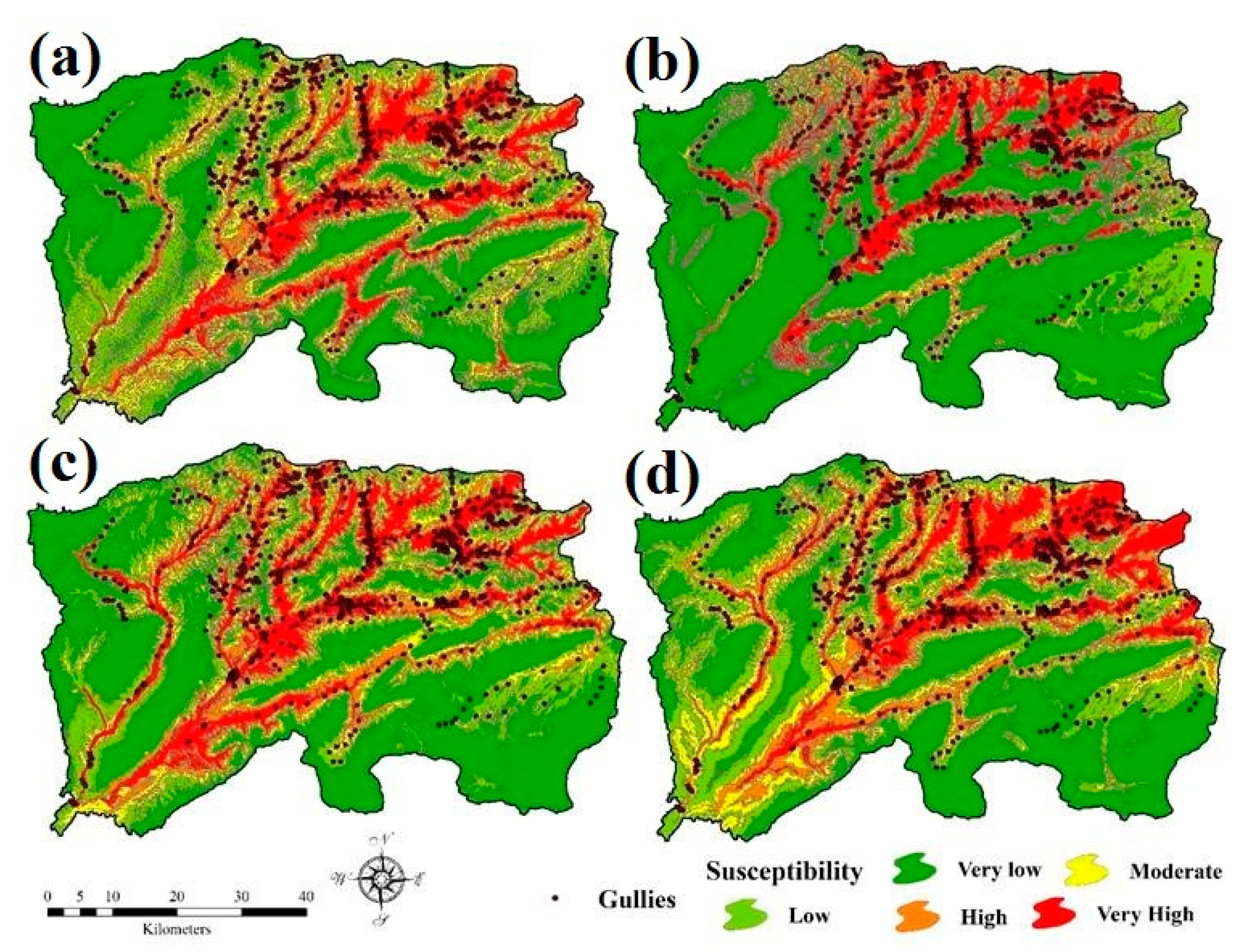
3.2. Gully Erosion Modeling with Individual Models
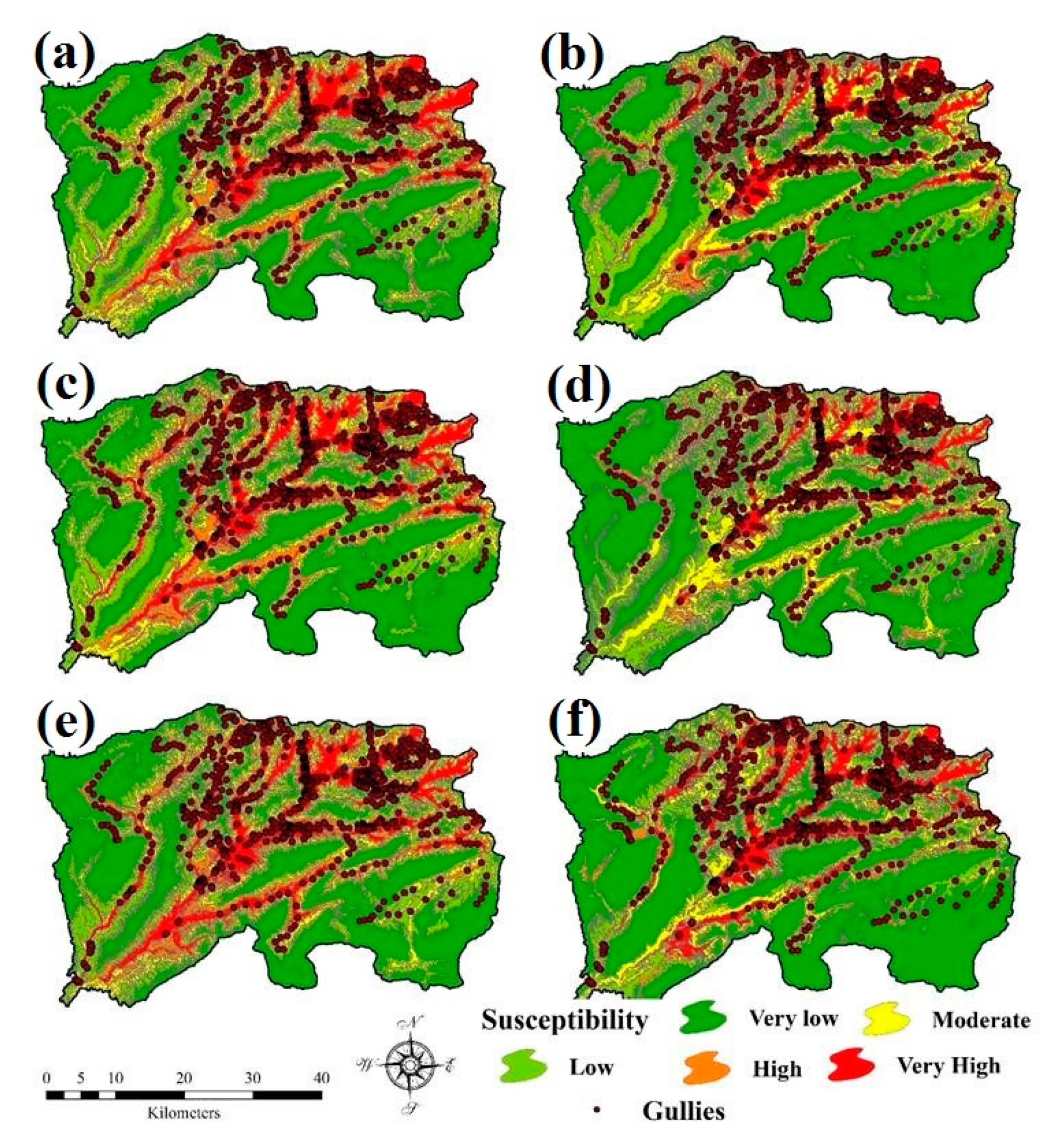
3.3. Gully Erosion Modeling by Ensemble of Two Models
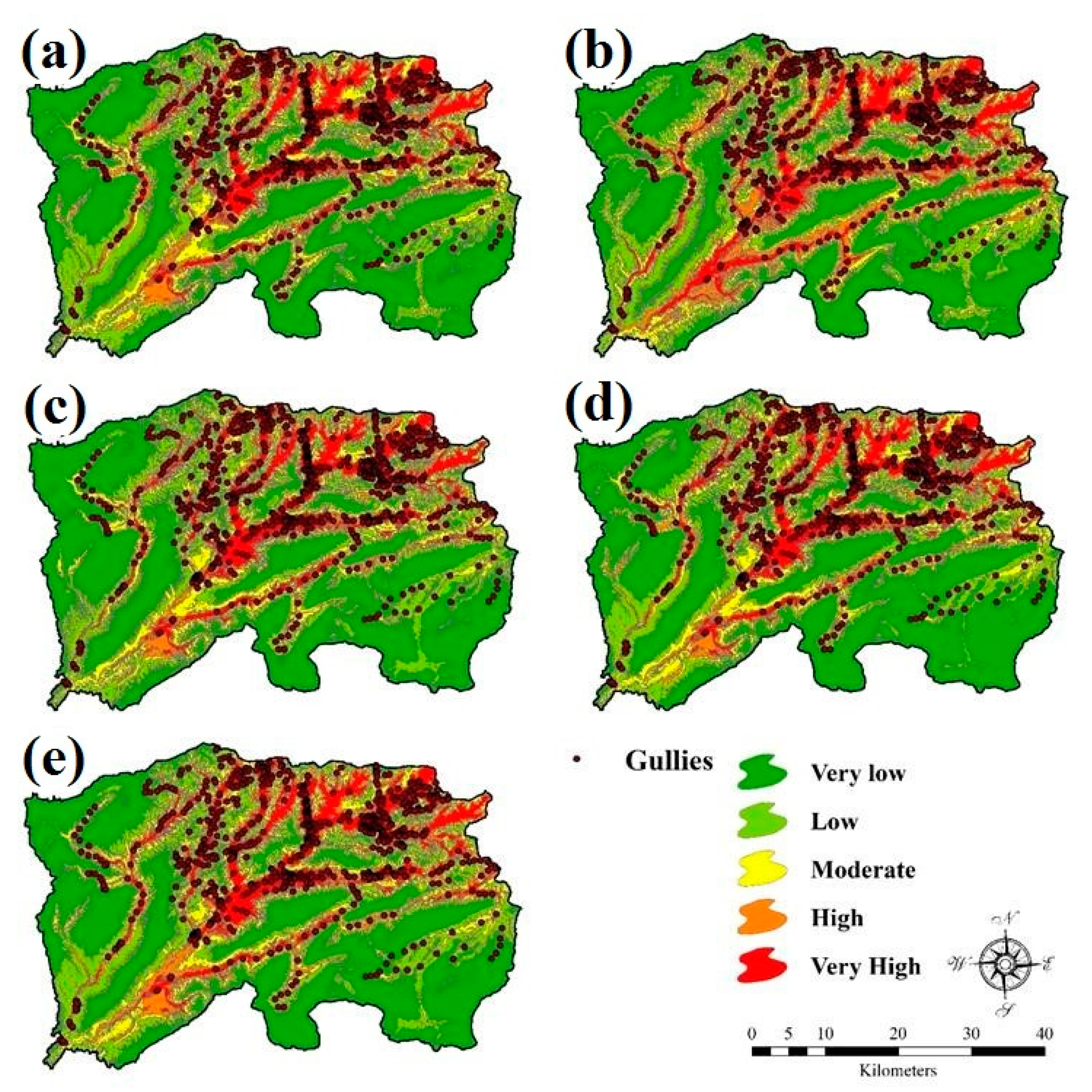
3.4. Gully Erosion Modeling by Ensemble of Three and Four Models
3.5. Assessing the Importance of the Factors
3.6. Validation of the Models
4. Discussion
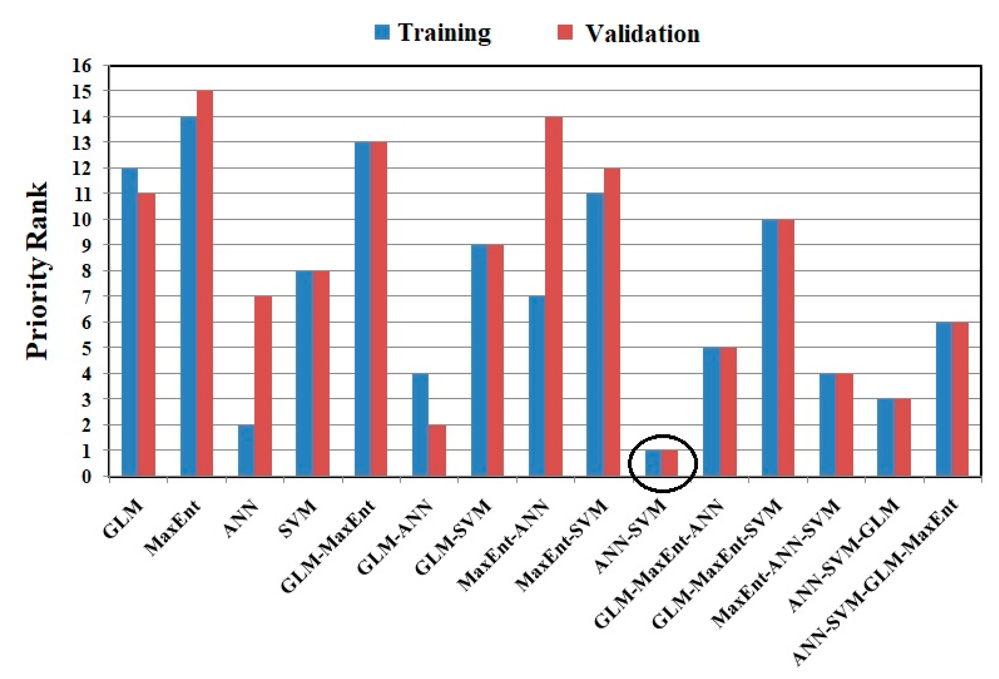
Models Prioritization
5. Conclusions
Author Contributions
Funding
Acknowledgments
Conflicts of Interest
References
- Ul Zaman, M.; Bhat, S.; Sharma, S.; Bhat, O. Methods to control soil erosion-a review. Int. J. Pure Appl. Biosci. 2018, 6, 1114–1121. [Google Scholar] [CrossRef]
- Parlak, M. Determination of erosion risk according to CORINE methodology (a case study: Kurtboğazı Dam). Int. Congr. River Basin Manag. 2007, 1, 856. [Google Scholar]
- Swarnkar, S.; Malini, A.; Tripathi, S.; Sinha, R. Assessment of uncertainties in soil erosion and sediment yield estimates at ungauged basins: An application to the Garra River basin, India. Hydrol. Earth Syst. Sci. 2018, 22, 2471–2485. [Google Scholar] [CrossRef] [Green Version]
- Arabameri, A.; Pradhan, B.; Pourghasemi, H.R.; Rezaei, K. Identification of erosion-prone areas using different multi-criteria decision-making techniques and GIS. Geomat. Nat. Haz. Risk 2018, 9, 1129–1155. [Google Scholar] [CrossRef] [Green Version]
- Arabameri, A.; Pourghasemi, H.R. Spatial modeling of gully erosion using linear and quadratic discriminant analyses in GIS and R. In Spatial Modeling in GIS and R for Earth and Environmental Sciences, 1st ed.; Pourghasemi, H.R., Gokceoglu, C., Eds.; Elsevier Publication: Amsterdam, The Netherlands, 2019. [Google Scholar] [CrossRef]
- Singh, O.; Singh, J. Soil Erosion Susceptibility Assessment of the Lower Himachal Himalayan Watershed. J. Geol. Soc. India 2018, 92, 157–165. [Google Scholar] [CrossRef]
- Odunuga, S.; Ajijola, A.; Igwetu, N.; Adegun, O. Land susceptibility to soil erosion in Orashi Catchment, Nnewi South, Anambra State, Nigeria. Proc. Int. Assoc. Hydrol. Sci. 2018, 376, 87–95. [Google Scholar] [CrossRef] [Green Version]
- Magliulo, P. Assessing the susceptibility to water-induced soil erosion using a geomorphological, bivariate statistics-based approach. Environ. Earth Sci. 2012, 67, s1801–s1820. [Google Scholar] [CrossRef]
- Arabameri, A.; Pourghasemi, H.R.; Yamani, M. Applying different scenarios for landslide spatial modeling using computational intelligence methods. Environ. Earth Sci. 2017, 76. [Google Scholar] [CrossRef]
- Arabameri, A.; Pourghasemi, H.R.; Cerda, A. Erodibility prioritization of subwatersheds using morphometric parameters analysis and its mapping: A comparison among TOPSIS, VIKOR, SAW, and CF multi-criteria decision making models. Sci. Total Environ. 2017, 613–614, 1385–1400. [Google Scholar] [CrossRef]
- Arabameri, A.; Rezaei, K.; Pourghasemi, H.R.; Lee, S.; Yamani, M. GIS-based gully erosion susceptibility mapping: A comparison among three data-driven models and AHP knowledge-based technique. Environ. Earth Sci. 2018, 77, 628. [Google Scholar] [CrossRef]
- Sun, W.; Shao, Q.; Liu, J.; Zhai, J. Assessing the effects of land use and topography on soil erosion on the Loess Plateau in China. Catena 2014, 121, 151–163. [Google Scholar] [CrossRef]
- Alam, M.; Hussain, R.R.; Islam, A.S. Impact assessment of rainfall-vegetation on sedimentation and predicting erosion-prone region by GIS and RS. Geomat. Nat. Hazards Risk 2016, 7, 667–679. [Google Scholar] [CrossRef] [Green Version]
- Li, H.; Cruse, R.M.; Bingner, R.L.; Gesch, K.R.; Zhang, X. Evaluating ephemeral gully erosion impact on Zea mays L. yield and economics using AnnAGNPS. Soil Tillage Res. 2016, 155, 157–165. [Google Scholar] [CrossRef]
- Saha, S.; Gayen, A.; Pourghasemi, H.R.; Tiefenbacher, J.P. Identification of soil erosion-susceptible areas using fuzzy logic and analytical hierarchy process modeling in an agricultural watershed of Burdwan district, India. Environ. Earth Sci. 2019, 78, 649. [Google Scholar] [CrossRef]
- Refahi, H. Soil Erosion by Water & Conservation; Tehran University Press: Tehran, Iran, 2009; pp. 10–202, (In Farsi with English Summary). [Google Scholar]
- Ezechi, J.I. The Influence of Runoff, Lithology and Water Table on the Dimensions and Rate of Gullying Processes in Eastern, Nigeria; Elsevier: Cremlingen, Germany, 2000. [Google Scholar]
- Paolo, P.; Desmond, W.E.; Antonina, C. Using 137 CS and 210 Pbex measurements and conventional surveys to investigate the relative contributions of inter rill/rill and gully erosion to soil loss from a small cultivated catchment in Sicily. Soil Tillage Res. 2014, 135, 18–27. [Google Scholar] [CrossRef]
- Arabameri, A.; Pradhan, B.; Bui, D.T. Spatial modelling of gully erosion in the Ardib River Watershed using three statistical-based techniques. Catena 2020, 190, 104545. [Google Scholar] [CrossRef]
- Arabameri, A.; Cerda, A.; Pradhan, B.; Tiefenbacher, J.P.; Lombardo, L.; Bui, D.T. A methodological comparison of head-cut based gully erosion susceptibility models: Combined use of statistical and artificial intelligence. Geomorphology 2020, 107136. [Google Scholar] [CrossRef]
- Zabihi, M.; Mirchooli, F.; Motevalli, A.; Darvishan, A.K.; Pourghasemi, H.R.; Zakeri, M.A.; Sadighi, F. Spatial modelling of gully erosion in Mazandaran Province, northern Iran. Catena 2018, 161, 1–13. [Google Scholar] [CrossRef]
- Arabameri, A.; Pradhan, B.; Rezaei, K.; Conoscenti, C. Gully erosion susceptibility mapping using GIS-based multi-criteria decision analysis techniques. Catena 2019, 180, 282–297. [Google Scholar] [CrossRef]
- Arabameri, A.; Chen, W.; Loche, M.; Zhao, X.; Li, Y.; Lombardo, L.; Cerda, A.; Pradhan, B.; Bui, D.T. Comparison of machine learning models for gully erosion susceptibility mapping. Geosci. Front. 2019. [Google Scholar] [CrossRef]
- Arabameri, A.; Pradhan, B.; Rezaei, K. Gully erosion zonation mapping using integrated geographically weighted regression with certainty factor and random forest models in GIS. J. Environ. Manag. 2019, 232, 928–942. [Google Scholar] [CrossRef]
- Zakerinejad, R.; Maerker, M. An integrated assessment of soil erosion dynamics with special emphasis on gully erosion in the Mazayjan basin, southwestern Iran. Nat. Hazards 2015, 79, 25–50. [Google Scholar] [CrossRef]
- Shit, P.K.; Paira, R.; Bhunia, G.; Maiti, R. Modeling of potential gully erosion hazard using geo-spatial technology at Garbheta block, West Bengal in India. Modeling Earth Syst. Environ. 2015, 1, 1–16. [Google Scholar] [CrossRef]
- Ganasri, B.P.; Ramesh, H. Assessment of soil erosion by RUSLE model using remote sensing and GIS-A case study of Nethravathi Basin. Geosci. Front. 2016, 7, 953–961. [Google Scholar] [CrossRef] [Green Version]
- Arekhi, S.; Niazi, Y. Assessment of GIS and RS applications to estimate soil erosion and sediment loading by using RUSLE model (Case Study: Upstream basin of Ilam dam). J. Soil Water Conserv. 2010, 17, 1–27. [Google Scholar]
- Roy, J.; Saha, S. Assessment of land suitability for the paddy cultivation using analytical hierarchical process (AHP): A study on Hinglo river basin, Eastern India. Modeling Earth Syst. Environ. 2018, 4, 601–618. [Google Scholar] [CrossRef]
- Rahmati, O.; Haghizadeh, A.; Pourghasemi, H.R.; Noormohamadi, F. Gully erosion susceptibility mapping: The role of GIS-based bivariate statistical models and their comparison. Nat. Hazards 2016, 82, 1231–1258. [Google Scholar] [CrossRef]
- Conforti, M.; Aucelli, P.P.; Robustelli, G.; Scarciglia, F. Geomorphology and GIS analysis formapping gully erosion susceptibility in the Turbolo streamcatchment (Northern Calabria, Italy). Nat. Hazards 2011, 56, 881–898. [Google Scholar] [CrossRef]
- Mojaddadi, H.; Pradhan, B.; Nampak, H.; Ahmad, N.; Ghazali, A.H. Ensemble machine-learning-based geospatial approach for flood risk assessment using multisensory remote-sensing data and GIS. Geomat. Nat. Hazards Risk 2017, 8, 1080–1102. [Google Scholar] [CrossRef] [Green Version]
- Azareh, A.; Rahmati, O.; Rafiei-Sardooi, E.; Sankey, J.B.; Lee, S.; Shahabi, H.; Bin Ahmad, B. Modelling gully-erosion susceptibility in a semi-arid region, Iran: Investigation of applicability of certainty factor and maximum entropy models. Sci. Total Environ. 2019, 655, 684–696. [Google Scholar] [CrossRef]
- Aghdam, I.N.; Varzandeh, M.H.M.; Pradhan, B. Landslide susceptibility mappingusing an ensemble statistical index (Wi) and adaptive neuro-fuzzy inference system (ANFIS) model at Alborz Mountains (Iran). Environ. Earth Sci. 2016, 75, 553. [Google Scholar] [CrossRef]
- Kornejady, A.; Heidari, K.; Nakhavali, M. Assessment of landslide susceptibility, semi-quantitative risk and management in the Ilam dam basin Ilam, Iran. Environ. Resour. Res. 2015, 3, 85–109. [Google Scholar] [CrossRef]
- Dube, F.; Nhapi, I.; Murwira, A.; Gumindoga, W.; Goldin, J.; Mashauri, D.A. Potential of weight of evidence modelling for gully erosion hazard assessment in Mbire District—Zimbabwe. Phys. Chem. Earth 2014, 67, 145–152. [Google Scholar] [CrossRef]
- Zakerinejad, R.; Maerker, M. Prediction of gully erosion susceptibilities using detailed terrain analysis and maximum entropy modeling: A case study in the Mazayejan Plain, Southwest Iran. Geogr. Fis. Din. Quat. 2014, 37, 67–76. [Google Scholar] [CrossRef]
- Gómez-Gutiérrez, Á.; Conoscenti, C.; Angileri, S.E.; Rotigliano, E.; Schnabel, S. Using topographical attributes to evaluate gully erosion proneness (susceptibility) in two Mediterranean basins: Advantages and limitations. Nat. Hazards 2015, 79, 291–314. [Google Scholar] [CrossRef]
- Pradhan, B.; Lee, S. Regional landslide susceptibility analysis using backpropagation neural network model at Cameron Highland, Malaysia. Landslides 2010, 7, 13–30. [Google Scholar] [CrossRef]
- Dehnavi, A.; Aghdam, I.N.; Pradhan, B.; Varzandeh, M.H.M. A new hybrid model using step-wise weight assessment ratio analysis (SWARA) technique and adaptive neuro-fuzzy inference system (ANFIS) for regional landslide hazard assessment in Iran. Catena 2015, 135, 122–148. [Google Scholar] [CrossRef]
- Amiri, M.; Pourghasemi, H.R.; Ghanbarian, G.A.; Afzali, S.F. Assessment of the importance of gully erosion effective factors using Boruta algorithm and its spatial modeling and mapping using three machine learning algorithms. Geoderma 2019, 340, 55–69. [Google Scholar] [CrossRef]
- Arabameri, A.; Pradhan, B.; Rezaei, K.; Yamani, M.; Pourghasemi, H.R.; Lombardo, L. Spatial modelling of gully erosion using evidential belief function, logistic regression, and a new ensemble of evidential belief function–logistic regression algorithm. Land Degrad. Dev. 2018, 29, 4035–4049. [Google Scholar] [CrossRef]
- Hosseinalizadeh, M.; Kariminejad, N.; Chen, W.; Pourghasemi, H.R.; Alinejad, M.; Behbahani, A.M.; Tiefenbacher, J.P. Spatial modelling of gully headcuts using UAV data and four best-first decision classifier ensembles (BFTree, Bag-BFTree, RS-BFTree, and RF-BFTree). Geomorphology 2019, 329, 184–193. [Google Scholar] [CrossRef]
- Roy, J.; Saha, S. GIS-based Gully Erosion Susceptibility Evaluation Using Frequency Ratio, Cosine Amplitude and Logistic Regression Ensembled with fuzzy logic in Hinglo River Basin, India. Remote Sens. Appl. Soc. Environ. 2019, 15, 100247. [Google Scholar] [CrossRef]
- Pourghasemi, H.R.; Yourself, S.; Kornejady, A.; Cerdà, A. Performance assessment of individual and ensemble data-mining techniques for gully erosion modeling. Sci. Total Environ. 2017, 609, 764–775. [Google Scholar] [CrossRef] [Green Version]
- Chen, W.; Pourghasemi, H.R.; Kornejady, A.; Zhang, N. Landslide spatial modeling: Introducing new ensembles of ANN, MaxEnt, and SVM machine learning techniques. Geoderma 2017, 305, 314–327. [Google Scholar] [CrossRef]
- Pham, B.T.; Bui, D.T.; Prakash, I.; Dholakia, M.B. Hybrid integration of Multilayer Perceptron Neural Networks and machine learning ensembles for landslide susceptibility assessment at Himalayan area (India) using GIS. Catena 2017, 149, 52–63. [Google Scholar] [CrossRef]
- Arabameri, A.; Yamani, M.; Pradhan, B.; Melesse, A.; Shirani, K.; Bui, D.T. Novel ensembles of COPRAS multi-criteria decision-making with logistic regression, boosted regression tree, and random forest for spatial prediction of gully erosion susceptibility. Sci. Total Environ. 2019, 688, 903–916. [Google Scholar] [CrossRef] [PubMed]
- Arabameri, A.; Pradhan, B.; Rezaei, K. Spatial prediction of gully erosion using ALOS PALSAR data and ensemble bivariate and data mining models. Geosci. J. 2019, 23, 669–686. [Google Scholar] [CrossRef]
- Chen, W.; Li, H.; Hou, E.; Wang, S.; Wang, G.; Panahi, M.; Li, T.; Peng, T.; Guo, C.; Niu, C.; et al. GIS-based groundwater potential analysis using novel ensemble weights-of-evidence with logistic regression and functional tree models. Sci. Total Environ. 2018, 634, 853–867. [Google Scholar] [CrossRef] [Green Version]
- Arabameri, A.; Pradhan, B.; Lombardo, L. Comparative assessment using boosted regression trees, binary logistic regression, frequency ratio and numerical risk factor for gully erosion susceptibility modelling. Catena 2019, 183, 104223. [Google Scholar] [CrossRef]
- Arabameri, A.; Chen, W.; Blaschke, T.; Tiefenbacher, J.P.; Pradhan, B.; Tien Bui, D. Gully Head-Cut Distribution Modeling Using Machine Learning Methods—A Case Study of NW Iran. Water 2020, 12, 16. [Google Scholar] [CrossRef] [Green Version]
- Arabameri, A.; Chen, W.; Lombardo, L.; Blaschke, T.; Tien Bui, D. Hybrid computational intelligence models for improvement gully erosion assessment. Remote Sens. 2020, 12, 140. [Google Scholar] [CrossRef] [Green Version]
- Arabameri, A.; Pradhan, B.; Rezaei, K.; Lee, C.W. Assessment of landslide susceptibility using statistical-and artificial intelligence-based FR–RF integrated model and multiresolution DEMs. Remote Sens. 2019, 11, 999. [Google Scholar] [CrossRef] [Green Version]
- Arabameri, A.; Cerda, A.; Rodrigo-Comino, J.; Pradhan, B.; Sohrabi, M.; Blaschke, T.; Tien Bui, D. Proposing a novel predictive technique for gully erosion susceptibility mapping in arid and semi-arid regions (Iran). Remote Sens. 2019, 11, 2577. [Google Scholar] [CrossRef] [Green Version]
- Arabameri, A.; Cerda, A.; Tiefenbacher, J.P. Spatial pattern analysis and prediction of gully erosion using novel hybrid model of entropy-weight of evidence. Water 2019, 11, 1129. [Google Scholar] [CrossRef] [Green Version]
- Zerihun, M.; Mohammedyasin, M.S.; Sewnet, D.; Adem, A.A.; Lakew, M. Assessment of soil erosion using RUSLE, GIS and remote sensing in NW Ethiopia. Geoderma Reg. 2018, 12, 83–90. [Google Scholar] [CrossRef]
- Islamic Republic of Iran Meteorological Organization (IRIMO). 2012. Available online: http://www.mazandaranmet.ir (accessed on 12 August 2018).
- IUSS Working Group WRB. World Reference Base for Soil Resources 2014; World Soil Resources Report; FAO: Rome, Italy, 2014. [Google Scholar]
- Saha, S.; Roy, J.; Arabameri, A.; Blaschke, T.; Tien Bui, D. Machine learning-based gully erosion susceptibility mapping: A case study of Eastern India. Sensors 2020, 20, 1313. [Google Scholar] [CrossRef] [Green Version]
- Conoscenti, C.; Angileri, S.; Cappadonia, C.; Rotigliano, E.; Agnesi, V.; Marker, M. Gully erosion susceptibility assessment by means of GIS-based logistic regression: A case of Sicily (Italy). Geomorphology 2014, 204, 399–411. [Google Scholar] [CrossRef] [Green Version]
- Cama, M.; Lombardo, L.; Conoscenti, C.; Rotigliano, E. Improving transferability strategies for debris flow susceptibility assessment: Application to the Saponara and Itala catchments (Messina, Italy). Geomorphology 2017, 288, 52–65. [Google Scholar] [CrossRef]
- Garosi, Y.; Sheklabadi, M.; Pourghasemi, H.R.; Besalatpour, A.A.; Conoscenti, C.; Van Oost, K. Comparison of differences in resolution and sources of controlling factors for gully erosion susceptibility mapping. Geoderma 2018, 330, 65–78. [Google Scholar] [CrossRef]
- Ollobarren Del Barrio, P.; Campo-Bescós, M.A.; Giménez, R.; Casalí, J. Assessment of soil factors controlling ephemeral gully erosion on agricultural fields. Earth Surf. Process. Landf. 2018, 43, 1993–2008. [Google Scholar] [CrossRef] [Green Version]
- Kheir, R.B.; Wilson, J.; Deng, Y. Use of terrain variables for mapping gully erosion susceptibility in Lebanon. Earth Surf. Process. Landf. 2007, 32, 1770–1782. [Google Scholar] [CrossRef]
- Montgomery, D.R.; Dietrich, W.E. Channel initiation and the problem of landscape scale. Science 1992, 255, 826. [Google Scholar] [CrossRef] [PubMed] [Green Version]
- Parras-Alcántara, L.; Lozano-García, B.; Keesstra, S.; Cerdà, A.; Brevik, E.C. Long-term effects of soil management on ecosystem services and soil loss estimation in olive grove top soils. Sci. Total Environ. 2016, 571, 498–506. [Google Scholar] [CrossRef] [PubMed]
- Poesen, J.; Nachtergaele, J.; Verstraeten, G.; Valentin, C. Gully erosion and environmental change: Importance and research needs. Catena 2003, 50, 91–133. [Google Scholar] [CrossRef]
- Boreggio, M.; Bernard, M.; Gregoretti, C. Evaluating the influence of gridding techniques for Digital Elevation Models generation on the debris flow routing modeling: A case study from Rovina di Cancia basin (North-eastern Italian Alps). Front. Earth Sci. 2018, 6, 89. [Google Scholar] [CrossRef] [Green Version]
- Gesch, D.; Oimoen, M.; Zhang, Z.; Meyer, D.; Danielson, J. Validation of the ASTER global digital elevation model version 2 over the conterminous United States. Int. Arch. Photogramm. Remote Sens. Spat. Inf. Sci. 2012, 39, 281–286. [Google Scholar] [CrossRef] [Green Version]
- Zhou, C.; Ge, L.E.D.; Chang, H.C. A case study of using external DEM in InSAR DEM generation. Geo-Spat. Inf. Sci. 2005, 8, 14–18. [Google Scholar] [CrossRef] [Green Version]
- Zhang, W.; Wang, W.; Chen, L. Constructing DEM based on InSAR and the relationship between InSAR DEM’s precision and terrain factors. Energy Procedia 2012, 16, 184–189. [Google Scholar] [CrossRef] [Green Version]
- Conoscenti, C.; Agnesi, V.; Cama, M.; Caraballo-Arias, N.A.; Rotigliano, E. Assessment of gully erosion susceptibility using multivariate adaptive regression splines and accounting for terrain connectivity. Land Degrad. Dev. 2018, 29, 724–736. [Google Scholar] [CrossRef]
- Ghorbani Nejad, S.; Falah, F.; Daneshfar, M.; Haghizadeh, A.; Rahmati, O. Delineation of groundwater potential zones using remote sensing and GIS-based data-driven models. Geocarto Int. 2016. [Google Scholar] [CrossRef]
- Jaafari, A.; Najafi, A.; Pourghasemi, H.R.; Rezaeian, J.; Sattarian, A. GIS–based frequency ratio and index of entropy models for landslide susceptibility assessment in the Caspian forest, northern Iran. Int. J. Environ. Sci. Technol. 2014, 11, 909–926. [Google Scholar] [CrossRef] [Green Version]
- Nobre, A.D.; Cuartas, L.A.; Hodnett, M.; Rennó, C.D.; Rodrigues, G.; Silveira, A.; Waterloo, M.; Saleska, S. Height above the nearest drainage—A hydrologically relevant new terrain model. J. Hydrol. 2011, 404, 13–29. [Google Scholar] [CrossRef] [Green Version]
- Kornejady, A.; Ownegh, M.; Bahremand, A. Landslide susceptibility assessment using maximum entropy model with two different data sampling methods. Catena 2017, 152, 144–162. [Google Scholar] [CrossRef]
- Rahmati, O.; Moghaddam, D.D.; Moosavi, V.; Kalantari, Z.; Samadi, M.; Lee, S.; Tien Bui, D. An automated python language-based tool for creating absence samples in groundwater potential mapping. Remote Sens. 2019, 11, 1375. [Google Scholar] [CrossRef] [Green Version]
- Liao, Y.; Yuan, Z.; Zhuo, M.; Huang, B.; Nie, X.; Xie, Z.; Tang, C.; Li, D. Coupling effects of erosion and surface roughness on colluvial deposits under continuous rainfall. Soil Tillage Res. 2019, 191, 98–107. [Google Scholar] [CrossRef]
- Boer, E.P.; de Beurs, K.M.; Hartkamp, A.D. Kriging and thin plate splines for mapping climate variables. Int. J. Appl. Earth Obs. Geoinf. 2001, 3, 146–154. [Google Scholar] [CrossRef]
- Beach, T. The fate of eroded soil: Sediment sinks and sediment budgets of agrarian landscapes in Southern Minnesota, 1851–1988. Ann. Assoc. Am. Geogr. 1994, 84, 5–28. [Google Scholar] [CrossRef]
- Nyssen, J.; Poesen, J.; Moeyersons, J.; Luyten, E.; Veyret-Picot, M.; Deckers, J.; Haile, M.; Govers, G. Impact of road building on gully erosion risk: A case study from the northern Ethiopian highlands. Earth Surf. Process. Landf. J. Br. Geomorphol. Res. Group 2002, 27, 1267–1283. [Google Scholar] [CrossRef]
- Bean, T.; Sumner, P.; Boojhawon, R.; Tatayah, V.; Khadun, A.; Hedding, D.W.; Rughooputh, S.D.D.V.; Nel, W. Bedrock-incised gully erosion phenomena on Round Island, Mauritius. Catena 2017, 151, 107–117. [Google Scholar] [CrossRef]
- Geology Survey of Iran (GSI). 1997. Available online: http://www.gsi.ir/Main/Lang_en/index.html (accessed on 5 June 2020).
- Maestre, F.T.; Cortina, J. Spatial patterns of surface soil properties and vegetation in a Mediterranean semiarid steppe. Plant Soil 2002, 241, 279–291. [Google Scholar] [CrossRef]
- Zucca, C.; Canu, A.; Della Peruta, R. Effects of land use and landscape on spatial distribution and morphological features of gullies in an agropastoral area in Sardinia (Italy). Catena 2006, 68, 87–95. [Google Scholar] [CrossRef]
- Phillips, S.J.; Dudík, M.; Elith, J.; Graham, C.H.; Lehmann, A.; Leathwick, J.; Ferrier, S. Sample selection bias and presence-only distribution models: Implications for background and pseudo-absence data. Ecol. Appl. 2009, 19, 181–197. [Google Scholar] [CrossRef] [Green Version]
- Keesstra, S.; Pereira, P.; Novara, A.; Brevik, E.C.; Azorin-Molina, C.; Parras-Alcántara, L.; Jordán, A.; Cerdà, A. Effects of soil management techniques on soil water erosion in apricot orchards. Sci. Total Environ. 2016, 551, 357–366. [Google Scholar] [CrossRef] [PubMed] [Green Version]
- Reddy, S.; Dávalos, L.M. Geographical sampling bias and its implications for conservation priorities in Africa. J. Biogeogr. 2003, 30, 1719–1727. [Google Scholar] [CrossRef]
- Shannon, C.E. Amathematical theory of communication. Bell Syst. Tech. J. 1948, 27, 379–423. [Google Scholar] [CrossRef] [Green Version]
- Elith, J.; Phillips, S.J.; Hastie, T.; Dudík, M.; Chee, Y.E.; Yates, C.J. A statistical explanation of MaxEnt for ecologists. Divers. Distrib. 2011, 17, 43–57. [Google Scholar] [CrossRef]
- Phillips, S.J.; Dudík, M.; Schapire, R.E. A maximum entropy approach to species distribution modeling. In Proceedings of the Twenty-First International Conference on Machine Learning, London, UK, 24 July 2004; p. 83. [Google Scholar]
- Jaynes, E.T. Information theory and statistical mechanics. Phys. Rev. 1957, 106, 620. [Google Scholar] [CrossRef]
- Jaynes, E.T. Information theory and statistical mechanics. II. Phys. Rev. 1957, 108, 171. [Google Scholar] [CrossRef]
- Cherkassky, V.; Krasnopolsky, V.; Solomatine, D.P.; Valdes, J. Computational intelligence in earth sciences and environmental applications: Issues and challenges. Neural Netw. 2006, 19, 113–121. [Google Scholar] [CrossRef]
- Peddle, D.R.; Foody, G.M.; Zhang, A.; Franklin, S.E.; LeDrew, E.F. Multi-source image classification II: An empirical comparison of evidential reasoning and neural network approaches. Can. J. Remote Sens. 1994, 20, 396–407. [Google Scholar] [CrossRef]
- Kosko, B. Neural Networks and Fuzzy Systems: A Dynamical Systems Approach to Machine Intelligence/Book and Disk; Prentice Hall: Upper Saddle River, NJ, USA, 1992. [Google Scholar]
- Falaschi, F.; Giacomelli, F.; Federici, P.R.; Puccinelli, A.; Avanzi, G.A.; Pochini, A.; Ribolini, A. Logistic regression versus artificial neural networks: Landslide susceptibility evaluation in a sample area of the Serchio River valley, Italy. Nat. Hazards 2009, 50, 551–569. [Google Scholar] [CrossRef]
- Gong, P.; Pu, R.; Chen, J. Elevation and forest-cover data using neural networks. Photogramm. Eng. Remote Sens. 1996, 62, 1249–1260. [Google Scholar]
- Arora, M.K.; Das Gupta, A.S.; Gupta, R.P. An artificial neural network approach for landslide hazard zonation in the Bhagirathi (Ganga) Valley, Himalayas. Int. J. Remote Sens. 2004, 25, 559–572. [Google Scholar] [CrossRef]
- Vapnik, V. The Nature of Statistical Learning Theory; Springer Science & Business Media: Berlin/Heidelberg, Germany, 2013. [Google Scholar]
- Cristianini, N.; Shawe-Taylor, J. An Introduction to Support Vector Machines and Other Kernel-Based Learning Methods; Cambridge University Press: Cambridge, UK, 2000. [Google Scholar]
- Joachims, T. Text categorization with support vector machines: Learning with many relevant features. In European Conference on Machine Learning; Springer: Berlin/Heidelberg, Germany, 1998; pp. 137–142. [Google Scholar]
- Burges, C.J. A tutorial on support vector machines for pattern recognition. Data Min. Knowl. Discov. 1998, 2, 121–167. [Google Scholar] [CrossRef]
- Kanevski, M.; Pozdnoukhov, A.; Timonin, V. Machine Learning for Spatial Environmental Data: Theory, Applications, and Software; EPFL Press: Lausanne, Switzerland, 2009. [Google Scholar]
- Marjanović, M.; Kovačević, M.; Bajat, B.; Voženílek, V. Landslide susceptibility assessment using SVM machine learning algorithm. Eng. Geol. 2011, 123, 225–234. [Google Scholar] [CrossRef]
- Hastie, T.; Tibshirani, R.; Friedman, J.H. The Elements of Statistical Learning: Data Mining, Inference, and Prediction; Springer: New York, NY, USA, 2001. [Google Scholar]
- Tax, D.M.; Duin, R.P. Support vector domain description. Pattern Recognit. Lett. 1999, 20, 1191–1199. [Google Scholar] [CrossRef]
- Pourghasemi, H.R.; Jirandeh, A.G.; Pradhan, B.; Xu, C.; Gokceoglu, C. Landslide susceptibility mapping using support vector machine and GIS at the Golestan Province, Iran. J. Earth Syst. Sci. 2013, 122, 349–369. [Google Scholar] [CrossRef] [Green Version]
- Poeppl, R.E.; Keesstra, S.D.; Maroulis, J. A conceptual connectivity framework for understanding geomorphic change in human-impacted fluvial systems. Geomorphology 2017, 277, 237–250. [Google Scholar] [CrossRef]
- McCullagh, P.; Nelder, J.A. Generalized Linear Models, 2nd ed.; Chapman and Hall/CRC: Boca Raton, FL, USA, 1989; p. 532. [Google Scholar]
- Payne, R. A Guide to Regression, Nonlinear and Generalized Linear Models in GenStat; VSN International: Hemel Hempstead, UK, 2012; p. 88. [Google Scholar]
- Bernknopf, R.L.; Brookshire, D.S.; Shapiro, C.D. A probabilistic approach to landslide hazard mapping in Cincinnati, Ohio, with applications for economic evaluation. Bull. Assoc. Eng. Geol. 1988, 24, 39–56. [Google Scholar] [CrossRef]
- Nikita, E. The use of generalized linear models and generalized estimating equations in bioarchaeological studies. Am. J. Phys. Anthropol. 2014, 153, 473–483. [Google Scholar] [CrossRef]
- Breiman, L. Random forests. Mach. Learn. 2001, 45, 5–32. [Google Scholar] [CrossRef] [Green Version]
- Breiman, L.; Friedman, J.H.; Olshen, R.A.; Stone, C.J. Classification and Regression Trees; Chapman & Hall: New York, NY, USA, 1984. [Google Scholar]
- Micheletti, N.; Foresti, L.; Robert, S.; Leuenberger, M.; Pedrazzini, A.; Jaboyedoff, M.; Kanevski, M. Machine learning feature selection methods for landslide susceptibility mapping. Math. Geosci. 2014, 46, 33–57. [Google Scholar] [CrossRef] [Green Version]
- Calle, M.L.; Urrea, V. Letter to the Editor: Stability of random forest importance measures. Brief. Bioinform. 2010, 12, 86–89. [Google Scholar] [CrossRef] [PubMed] [Green Version]
- Kumar, R.; Indrayan, A. Receiver operating characteristic (ROC) curve for medical researchers. Indian Pediatrics 2011, 48, 277–287. [Google Scholar] [CrossRef] [PubMed]
- Pepe, M.S. Receiver operating characteristic methodology. J. Am. Stat. Assoc. 2000, 95, 308–311. [Google Scholar] [CrossRef]
- Roy, J.; Saha, S.; Arabameri, A.; Blaschke, T.; Bui, D.T. A novel ensemble approach for Landslide Susceptibility Mapping (LSM) in Darjeeling and Kalimpong Districts, West Bengal, India. Remote Sens. 2019, 11, 2866. [Google Scholar] [CrossRef] [Green Version]
- Paul, G.C.; Saha, S.; Hembram, T.K. Application of the GIS-based probabilistic models for mapping the flood susceptibility in Bansloi Sub-basin of Ganga-Bhagirathi River and their comparison. Remote Sens. Earth Syst. Sci. 2019, 2, 120–146. [Google Scholar] [CrossRef]
- Saha, S. Groundwater potential mapping using analytical hierarchical process: A study on Md. Bazar Block of Birbhum District, West Bengal. Spat. Inf. Res. 2017. [Google Scholar] [CrossRef]
- Rahmati, O.; Golkarian, A.; Biggs, T.; Keesstra, S.; Mohammadi, F.; Daliakopoulos, I.N. Land subsidence hazard modeling: Machine learning to identify predictors and the role of human activities. J. Environ. Manag. 2019, 236, 466–480. [Google Scholar] [CrossRef]
- Rahmati, O.; Falah, F.; Naghibi, S.A.; Biggs, T.; Soltani, M.; Deo, R.C.; Cerdà, A.; Mohammadi, F.; Bui, D.T. Land subsidence modelling using tree-based machine learning algorithms. Sci. Total Environ. 2019, 672, 239–252. [Google Scholar] [CrossRef]
- Pourghasemi, H.R.; Mohammady, M.; Pradhan, B. Landslide susceptibility mapping using index of entropy and conditional probability models in GIS: Safarood Basin, Iran. Catena 2012, 97, 71–84. [Google Scholar] [CrossRef]
- Frattini, P.; Crosta, G.; Carrara, A. Techniques for evaluating the performance of landslide susceptibility models. Eng. Geol. 2010, 111, 62–72. [Google Scholar] [CrossRef]
- Tien Bui, D.; Tuan, T.A.; Klempe, H.; Pradhan, B.; Revhaug, I. Spatial prediction models for shallow landslide hazards: A comparative assessment of the efficacy of support vector machines, artificial neural networks, kernel logistic regression, and logistic model tree. Landslides 2016, 13, 361–378. [Google Scholar] [CrossRef]
- Fressard, M.; Thiery, Y.; Maquaire, O. Which data for quantitative landslide susceptibility mapping at operational scale? Case study of the Pays d’Auge plateau hillslopes (Normandy, France). Nat. Hazards Earth Syst. Sci. Discuss. 2014, 14, 569–588. [Google Scholar] [CrossRef] [Green Version]
- Arabameri, A.; Roy, J.; Saha, S.; Blaschke, T.; Ghorbanzadeh, O.; Tien Bui, D. Application of probabilistic and machine learning models for groundwater potentiality mapping in Damghan Sedimentary Plain, Iran. Remote Sens. 2019, 11, 3015. [Google Scholar] [CrossRef] [Green Version]
- Lipovetsky, S. Pareto 80/20 law: Derivation via random partitioning. Int. J. Math. Educ. Sci. Technol. 2009, 40, 271–277. [Google Scholar] [CrossRef]
- Choubin, B.; Moradi, E.; Golshan, M.; Adamowski, J.; Sajedi-Hosseini, F.; Mosavi, A. An ensemble prediction of flood susceptibility using multivariate discriminate analysis, classification and regression trees, and support vector machines. Sci. Total Environ. 2019, 651, 2087–2096. [Google Scholar] [CrossRef]
- Deo, R.C.; Tiwari, M.K.; Adamowski, J.F.; Quilty, J.M. Forecasting effective drought index using a wavelet extreme learning machine (W-ELM) model. Stoch. Environ. Res. Risk Assess. 2017, 31, 1211–1240. [Google Scholar] [CrossRef]
- Rokach, L. Ensemble-based classifiers. Artif. Intell. Rev. 2010, 33, 1–39. [Google Scholar] [CrossRef]
- Tien Bui, D.; Pradhan, B.; Revhaug, I.; Tran, C.T. A Comparative Assessment between the Application of Fuzzy Unordered Rules Induction Algorithm and J48 Decision Tree Models in Spatial Prediction of Shallow Landslides at Lang Son City; Springer International Publishing: Cam, Swiss, 2014. [Google Scholar]
- Borrelli, P.; Märker, M.; Panagos, P.; Schütt, B. Modeling soil erosion and river sediment yield for an intermountain drainage basin of the Central Apennines, Italy. Catena 2014, 114, 45–58. [Google Scholar] [CrossRef]
- Huang, Y.; Zhao, L. Review on landslide susceptibility mapping using support vector machines. Catena 2018, 165, 520–529. [Google Scholar] [CrossRef]
- Yao, X.; Tham, L.G.; Dai, F.C. Landslide susceptibility mapping based on support vector machine: A case study on natural slopes of Hong Kong, China. Geomorphology 2008, 101, 572–582. [Google Scholar] [CrossRef]
- Ahirwar, R.; Malik, M.S.; Shukla, J.P. Prioritization of sub-watersheds for soil and water conservation in parts of Narmada River through morphometric analysis using remote sensing and GIS. J. Geol. Soc. India 2019, 94, 515–524. [Google Scholar] [CrossRef]


| Land Use | Area (ha) | Area (%) |
|---|---|---|
| Moderate Range | 56,971.77 | 25.91 |
| Poor Range | 41,968.52 | 19.09 |
| Dry farming-Garden | 31,329.69 | 14.25 |
| Dry Farming | 24,647.25 | 11.21 |
| Dense Forest | 24,595.63 | 11.19 |
| Orchard | 12,381.7 | 5.63 |
| Moderate Forest | 8679.79 | 3.95 |
| Good Range | 6471.76 | 2.94 |
| Low Forest | 4486.76 | 2.04 |
| Flood Crossing | 3824.86 | 1.74 |
| Agriculture | 3666.75 | 1.67 |
| Residential Areas | 819.21 | 0.37 |
| Geo Unit | Description | Area (ha) | Area (%) |
|---|---|---|---|
| Kat | Olive green glauconitic sandstone and shale | 11,516.28 | 5.24 |
| Qsw | Swamp | 133,117.1 | 60.56 |
| Ksn | Grey to block shale and thin layers of siltstone and sandstone | 17,645.92 | 8.03 |
| Ekh | Olive—green shale and sandstone | 2644.15 | 1.2 |
| Qm | Swamp and marsh | 29,445.41 | 13.4 |
| Ksr | Ammonite bearing shale with interaction of orbitolin limestone | 12,242.8 | 5.57 |
| Jmz | Grey thick—bedded limestone and dolomite | 3253.9 | 1.48 |
| Jl | Light grey, thin—bedded to massive limestone | 9945.08 | 4.52 |
| Conditioning Factors | Collinearity Statistics | |
|---|---|---|
| Tolerance | VIF | |
| LULC | 0.923 | 1.083 |
| Drainage density | 0.911 | 1.098 |
| Distance to road | 0.906 | 1.104 |
| Valley depth | 0.854 | 1.171 |
| Relative Slope Position (RSP) | 0.765 | 1.307 |
| Geology | 0.743 | 1.346 |
| Rainfall | 0.654 | 1.529 |
| Road density | 0.645 | 1.550 |
| Slope length | 0.518 | 1.931 |
| Aspect | 0.465 | 2.151 |
| Distance to stream | 0.456 | 2.193 |
| Slope | 0.423 | 2.364 |
| Height Above the Nearest Drainage (HAND) | 0.384 | 2.604 |
| Elevation | 0.355 | 2.817 |
| Factor | Weight |
|---|---|
| Distance to road | 19.23 |
| LULC | 18.60 |
| Height Above the Nearest Drainage (HAND) | 17.03 |
| Rainfall | 16.13 |
| Valley depth | 15.34 |
| Distance to stream | 14.65 |
| Slope length | 14.42 |
| Stream density | 13.54 |
| Aspect | 11.85 |
| Elevation | 9.34 |
| Geology | 9.08 |
| Slope | 4.43 |
| Relative Slope Position (RSP) | 2.76 |
| Road density | 1.65 |
© 2020 by the authors. Licensee MDPI, Basel, Switzerland. This article is an open access article distributed under the terms and conditions of the Creative Commons Attribution (CC BY) license (http://creativecommons.org/licenses/by/4.0/).
Share and Cite
Arabameri, A.; Asadi Nalivan, O.; Saha, S.; Roy, J.; Pradhan, B.; Tiefenbacher, J.P.; Thi Ngo, P.T. Novel Ensemble Approaches of Machine Learning Techniques in Modeling the Gully Erosion Susceptibility. Remote Sens. 2020, 12, 1890. https://0-doi-org.brum.beds.ac.uk/10.3390/rs12111890
Arabameri A, Asadi Nalivan O, Saha S, Roy J, Pradhan B, Tiefenbacher JP, Thi Ngo PT. Novel Ensemble Approaches of Machine Learning Techniques in Modeling the Gully Erosion Susceptibility. Remote Sensing. 2020; 12(11):1890. https://0-doi-org.brum.beds.ac.uk/10.3390/rs12111890
Chicago/Turabian StyleArabameri, Alireza, Omid Asadi Nalivan, Sunil Saha, Jagabandhu Roy, Biswajeet Pradhan, John P. Tiefenbacher, and Phuong Thao Thi Ngo. 2020. "Novel Ensemble Approaches of Machine Learning Techniques in Modeling the Gully Erosion Susceptibility" Remote Sensing 12, no. 11: 1890. https://0-doi-org.brum.beds.ac.uk/10.3390/rs12111890