MODIS-Based Remote Estimation of Absorption Coefficients of an Inland Turbid Lake in China

Abstract

Optical complexity and various properties of Case 2 waters make it essential to derive inherent optical properties (IOPs) through an appropriate method. Based on field measured data of Lake Chaohu between 2009 and 2018, the quasi-analytical algorithm (QAA) was modified for the particular scenario of that lake to derive absorption coefficients based on the moderate-resolution imaging spectroradiometer (MODIS) bands. By changing the reference wavelength to longer ones and building a relationship between the value of spectral power for particle backscattering coefficient (Y), suspended particulate matter (SPM), and above-surface remote-sensing reflectance (R_rs), we improved the accuracy of the retrieval of total absorption coefficients. The absorption coefficients of gelbstoff and non-algal particulates (a_dg) and absorption coefficients of phytoplankton (a_ph) in Lake Chaohu were also derived by changing important parameters according to Lake Chaohu. The derived a_ph tend to be bigger than measured a_ph in this study, while derived a_dg tend to be smaller than measured data. We also used the corrected MODIS surface reflectance product (MOD09/MYD09) to calculate the a_ph(443), a_ph(645), and a_ph(678) by the model proposed in this study. It shows that in summer and autumn, a_ph tended to be higher in the northwestern part of Lake Chaohu, and were relatively lower in the spring and winter, which is similar to previous studies. Overall, our study provides an algorithm that is effectively used in the case of Lake Chaohu and applicable to the data obtained by MODIS, which can be used for further study to investigate the change law of absorption coefficients in long time series by applying MODIS data.

1. Introduction

The inversion of water color involves the derivation of inherent optical properties (IOPs) from apparent optical properties (AOPs). As a result, information about water constituents is retrieved from derived IOPs, such as concentrations of chlorophyll-a (Chl a), suspended sediments, and colored, dissolved organic matter (CDOM).

Recent studies have emphasized the importance of retrieving IOPs through remote sensing. Variations in IOPs can precisely indicate changes in water constituents and mass. AOPs refer to the parameters that vary with the change of illumination conditions, including water-leaving radiance (L_w), above-surface remote-sensing reflectance (R_rs)_, and so on [1]. The IOPs and light field together determine the AOPs. The inversion of the IOPs can be achieved by using the related algorithms from the AOPs. R_rs is one of the most important AOPs, which is determined by the IOPs of the water body and the geometric structure of the underwater light field. Through the IOPs (absorption and scattering), inherent nonlinear intrinsic correlations exist between the concentration of each component and the remote-sensing reflectance.

Solutions to accurately derive the optical properties remotely have been studied for many years, and scientists have proposed algorithms related to this subject. Empirical algorithms use certain regressions between the IOPs and the ratios of below-surface remote sensing reflectance (r_rs) or R_rs. The main advantage of such an algorithm is that data processing is simple and rapid, which is essential in retrieving information from satellite sensors. However, due to the lack of a certain physical foundation, empirical models often rely too much on field-measured data, which are limited by time and region. Therefore, the applicability of those algorithms may be limited and may result in errors in different areas [2]. A semi-analytical model is based on the radiative transfer equation between the water composition, IOPs, and AOPs. These algorithms are suitable for various water types and are much more accurate than empirical algorithms [3,4]. Based on the basic theory of optical properties and the spectral model of water bodies, the quantitative relationship between the substance concentration in water and the optical properties of the water body can be established, which is called an analytical model. This model can be used for the large-scale and long-term monitoring of water color and quality. However the theoretical research and data measurement in different waters have not reached a perfect, applicable level.

Extensive work has been conducted on the inversion of IOPs in China and abroad, and the inversion model has gradually progressed from the traditional empirical model to the semi-analytical model. Carder et al. [3,5] presented a moderate-resolution imaging spectroradiometer (MODIS) semi-analytical algorithm, which can use R_rs to retrieve IOPs including absorption and backscattering coefficients. Hoge and Lyon [6,7] created a linear matrix inversion model by using R_rs at 412, 490, and 555 nm and retrieved the IOPs of the water body. Doerffer built a retrieval procedure of suspended particulate matter (SPM), chlorophyll, and gelbstoff concentration based on neutral network [8]. Lee et al. [9] investigated a quasi-analytical algorithm (QAA) that can retrieve IOPs by using multi-band R_rs data. This algorithm is applicable to hyperspectral data and multi-band satellite sensor data that have been or will be launched, such as the coastal zone color scanner (CZCS), the sea-viewing, wide field-of-view sensor (SeaWiFS), and MODIS [9]. It is derived from the analytical, semi-analytical, and empirical formulas for oceanic and coastal waters. It was updated to QAA_v6 in the following years [10].

QAA is one of the mainstream models at present. It has the characteristics of high precision and fast operation speed and can be used to process large quantities of data. In recent years, many scholars in China have conducted research on the application of QAA in coastal waters in the country [11,12,13]. For inland Case 2 waters, whose optical properties are significantly influenced by mineral particles, CDOM, or microbubbles [14], Le et al. [15,16] validated and improved the QAA algorithm in Lake Taihu; the results showed that the reference wavelength has to be longer in turbid waters. Xie et al. [17] applied the QAA to the inversion of the IOPs of Lake Kuncheng. Domestic research on IOPs mainly focuses on the inversion of ocean IOPs and the backscattering coefficient of inland water, but the inversion of the absorption coefficient of inland water is less studied [18]. Although QAA is widely used, there are still many uncertainties in deriving optical properties for optically complex Case 2 waters [16,19,20]. Specifically, the reference wavelength and the empirical formulas do not work for inland Case 2 waters, especially for the case of Lake Chaohu, which is a lake of high turbidity, Chl a concentrations, and complicated optical properties.

This study aimed to provide a solution to derive IOPs of Lake Chaohu by applying MODIS data. The time resolution of MODIS is effective for further study to investigate the change law of IOPs of Lake Chaohu in the long time series. In this paper, the derived absorption coefficients and measured absorption coefficients were compared and analyzed. Thereafter, some test data were used to measure the accuracy of this algorithm. We hope that this algorithm can provide a viable solution by applying remote sensing to the inversion of water color in Lake Chaohu or other turbid lakes.

2. Data

2.1. Study Area

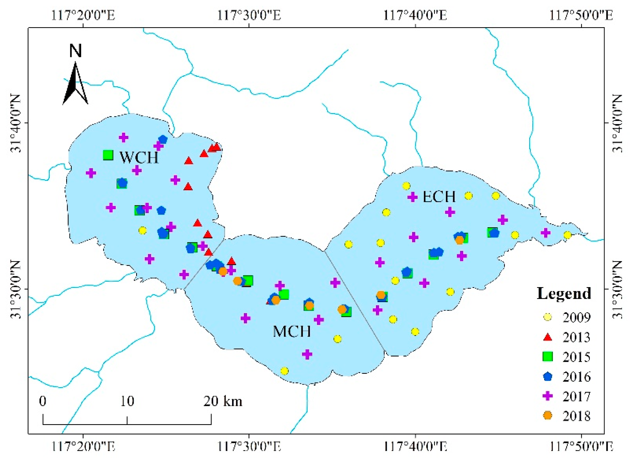
Lake Chaohu (31°25′–31°43′N, 117°17′–117°51′E, Figure 1) is an eutrophic and turbid shallow lake in Anhui Province, in the east of China, with an acreage of 770 km² and an average depth of 3.0 m [21]. This lake is an important source of fish and drinking water for Hefei, a city under a subtropical monsoon climate (Figure 1). Lake Chaohu has a volume of 32.3 × 10⁸ m³ during the rainy season for approximately five months and only 17.2 × 10⁸ m³ during the dry season for approximately seven months [22]. Around 9 million people live around the lake, in which the main contamination sources are agricultural, industrial, and municipal pollution [23,24]. Lake Chaohu has had poor water quality and frequent algal blooms, particularly cyanobacteria blooms, over the past few decades [25].

2.2. Sampling and Data Collection

We conducted 11 cruise surveys, with 119 surface samples from October 2009 to July 2018 to measure optical properties in Lake Chaohu in this study (Figure 1). From this, 94 samples were used to build models and 25 samples were used as test data. We measured R_rs data at the sites. The water samples were kept at 4 °C in the dark before experiments of SPM, Chl a, dissolved organic carbon concentration (DOC), and absorption coefficients.

Measurements of Relevant Parameters

A handheld ASD (analytical spectral device) under the NASA Ocean Optics protocols was used to obtain R_rs [26]. Applying the method described by Mobley et al. [27], the viewing direction was 40 degree from the nadir and 135 degree from the Sun.

We filtered the water samples by Whatman GF/C glass-fiber filters with a pore size of approximately 1.2 μm and extracted pigments with a reference of 90% acetone. We used a Shimadzu UV-2600 (Kyoto, Japan) to measure the absorbance then achieved Chl a data [28]. We pre-combusted Whatman GF/F glass-fiber filters with a pore size of 0.7 μm at 450 °C for 6 h and pre-weighed them. We then filtered the water samples and dried them at high temperature (105 °C) for approximately 4–6 h for the measurement of SPM concentrations. Suspended particulate inorganic matter (SPIM) was similarly measured through weighing the filters before and after burning organic matter for 6 h [29].

The absorption coefficients of total particulate matter, absorption coefficients of non-algal particulate (a_d), and absorption coefficients of phytoplankton (a_ph) at 350–800 nm were obtained by using the same machine with GF/F filters [26]. The baseline was obtained by a blank filter with distilled water [2]. The a_d was measured after the pigments were bleached with sodium hypochlorite, and then a_ph were derived. The absorption coefficient of CDOM (a_g) was measured using the same machine with Milli-Q water as the reference from water filtered by filters with a 0.22-μm pore size from 280 to 700 nm (1-nm interval) [2,30,31].

2.3. Satellite Image Data Preprocessing

In this study, MODIS data were selected as input data. MODIS has high spectral and time resolutions. It is set on Terra and Aqua and has five levels of data products. MODIS provides continuous global remote sensing data that have a wide range of applications in ecology and geography research. The MODIS data preprocessing in this study mainly refer to the geometric correction and atmospheric correction of the MODIS surface reflectance product (MOD09/MYD09) in Lake Chaohu.

2.3.1. The MOD09/MYD09 Product

The MOD09/MYD09 surface reflectance product can be used in the calculation of the Earth’s surface albedo [32,33]. It belongs to the terrestrial product and corresponds to the Terra and Aqua satellites, respectively. MOD09/MYD09 has reflectance data with 250-m resolution of Bands 1 and 2 (620–670 nm and 841–876 nm), 500-m resolution of Bands 1–7 (620–670 nm, 841–876 nm, 459–479 nm, 545–565 nm, 1230–1250nm, 1628–1652 nm, and 2105–2155 nm), 1-km resolution of Bands 1–16 (620–670 nm, 841–876 nm, 459–479 nm, 545–565 nm, 1230–1250 nm, 1628–1652 nm, 2105–2155 nm, 405–420 nm, 438–448 nm, 483–493 nm, 526–536 nm, 546–556 nm, 662–672 nm, 673–683 nm, 743–753 nm, and 862–877 nm), multi-resolution pixel state QA (quality assessment) data, and 1-km observation statistics. In the QA data, the type of ground cover is indicated. MOD09/MYD09 data (hereinafter referred to as MOD09) are based on Level1B data, which are corrected for the effects of low atmospheric gases and aerosols. Atmospheric correction aims to remove the impact of Sun glint, residual aerosol scattering, and so on. Given the requirements of lake water bodies for reflectance data, MOD09 data are still insufficient for Case 2 water body monitoring. In order to eliminate residual effects, further correction is needed.

2.3.2. The MOD09 Correction Method

The atmosphere is an important factor affecting the quantitative analysis and application of remote sensing. Therefore, removing the effects of atmospheric scattering and absorption from the radiance value received by the sensor has become the premise of remote sensing quantitative analysis. In some studies, MOD09 reflectance data are used directly [34,35,36]. Nevertheless, by comparing MOD09 data and measured data, it has been found that the MOD09 data generally show higher phenomena in some bands compared with the measured data [37].

In this study, we used a simple correction method based on near-infrared (NIR) and short-wave infrared (SWIR) bands [37]. The advantage of using this correction method is that it can eliminate the noise in MOD09 data by simple correction and then convert the surface reflectance to the scale of remote-sensing reflectance, so that a more accurate R_rs(λ) is obtained and can be more easily applied to processing. The specific correction method is as follows:

$${\mathrm{R}}_{\mathrm{r}\mathrm{s}}\left(\mathsf{\lambda }\right)=\frac{\mathrm{R}\left(\mathsf{\lambda }\right)-\min \left({\mathrm{R}}_{\mathrm{NIR}}:{\mathrm{R}}_{\mathrm{SWIR}}\right)}{\pi }$$

(1)

where min (R_NIR: R_SWIR) refers to the minimum reflectance value of NIR and SWIR bands. Due to the strong absorption of water in the NIR and SWIR bands, reflectance will generally drop to 0 in the NIR band in the case of general water, while reflectance will generally decrease to 0 in the SWIR band in the case of turbid water [38]. Therefore, the reflectance value of the NIR and SWIR bands is considered as additive noise. The additive noise can be eliminated by subtracting the value from each band value.

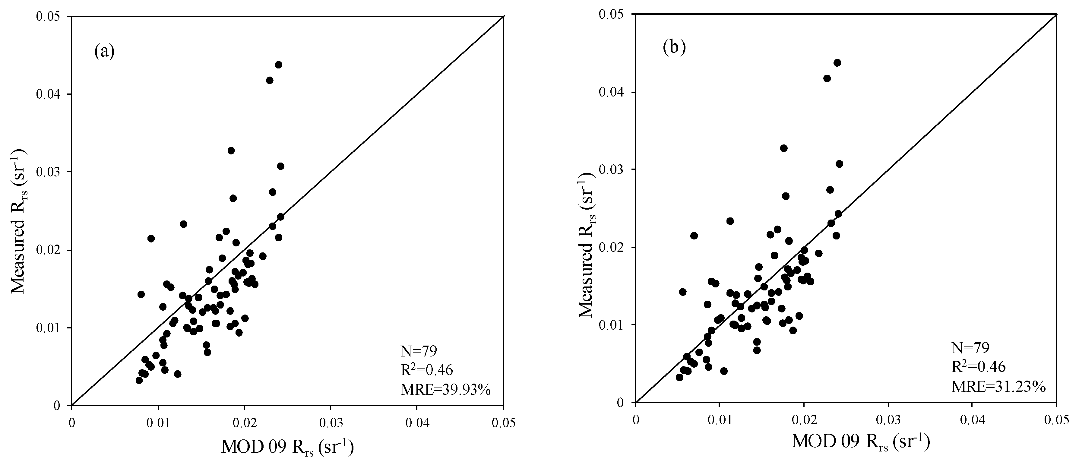
After the correction by this method, there are still some gaps between the corrected R_rs and the measured values at 748 nm (Figure 2a).Therefore, this study used the least-square method to calibrate the values at 748 nm, again based on the measured data. The equation between the measured R_rs and the values derived from MOD09 is constructed to make the values closer to the measured data. The R_rs after recalibration is shown in Figure 2b (N = 79). Similarly, the R_rs values at 413 and 443 nm were also corrected again using this method.

3. Improving QAA

QAA is a semi-analytical method for calculating the absorption coefficient and backscattering coefficient of water proposed by Lee et al. [9]. The inversion process of QAA has two parts. The first one is deriving the total absorption coefficient and backscattering coefficient. The second, utilizing the coefficient of the total absorption obtained from the first part, is decomposing the total absorption coefficient into different elements. The QAA algorithm is proposed for open ocean and coastal waters; accordingly, some empirical formulas are used for specific research areas, which cannot be directly applied to the inversion of the absorption coefficients for inland Case 2 waters.

3.1. Inversion of Total Absorption Coefficients

In the first part of QAA, a relationship between R_rs and total absorption coefficients was established. Similarly in this study, a new relationship needs to be established according to Lake Chaohu by changing some parameters and formulas as follows.

3.1.1. Values of g₀ and g₁

$$\mathrm{u}\left(\mathsf{\lambda }\right)=\frac{-{\mathrm{g}}_0+{[{({\mathrm{g}}_0)}^2+4{\mathrm{g}}_1{\mathrm{r}}_{\mathrm{r}\mathrm{s}}\left(\mathsf{\lambda }\right)]}^{1/2}}{2{\mathrm{g}}_1}$$

(2)

The ratio of backscattering coefficient to the sum of absorption and backscattering coefficients (u(λ)) is calculated by r_rs and g₀, g₁. Gordon et al. [39] found the values of g₀ = 0.0949 and g₁ = 0.0794 for oceanic Case 1 waters, whose optical properties are determined primarily by phytoplankton, CDOM, and detritus degradation products [40]. Lee et al. [9,41] advised that g₀ = 0.084 and g₁ = 0.17 is more accurate for higher-scattering coastal waters. In fact, the values of g₀ and g₁ are different because they depend on the particle phase function, which cannot be measured remotely. The values of these two parameters have to be estimated before being used in semi-analytical algorithms. Lee [9] used the averaged g₀ and g₁ values, which can be applied to coastal and open ocean waters. However, the values of g₀ and g₁ have a minimal influence on the inversion accuracy of the total absorption coefficient. Therefore, in this study, after trying to apply different values, we used the values of g₀ of 0.08945 and g₁ of 0.1247 as in the QAA original algorithm, which is suitable for more types of waters.

3.1.2. Reference Wavelength

The measurements of absorption coefficients of water constituents include a_ph(λ), a_d(λ), and a_g(λ). The total absorption coefficient a(λ) is the sum of a_ph(λ), a_d(λ), a_g(λ), and the absorption coefficient of pure water a_w(λ) [42].

a(λ) = a_ph(λ) + a_d(λ) + a_g(λ) + a_w(λ)

(3)

The principle of selecting the reference wavelength in Step 2 (QAA) is that the absorption coefficient of pure water is dominant at the reference wavelength, and a_w(λ₀) can basically replace a(λ₀).

Table 1. Reference wavelengths from different cases of waters.

Reference Wavelength	Areas	Reference
555 nm	oligotrophic waters mesotrophic waters	[9]
640 nm	high-absorbing waters	[9]
695 nm	Lake Kuncheng	[17]
715 nm	Lake Taihu, Chaohu	[15,43]

provides examples of reference wavelengths in some relevant studies.

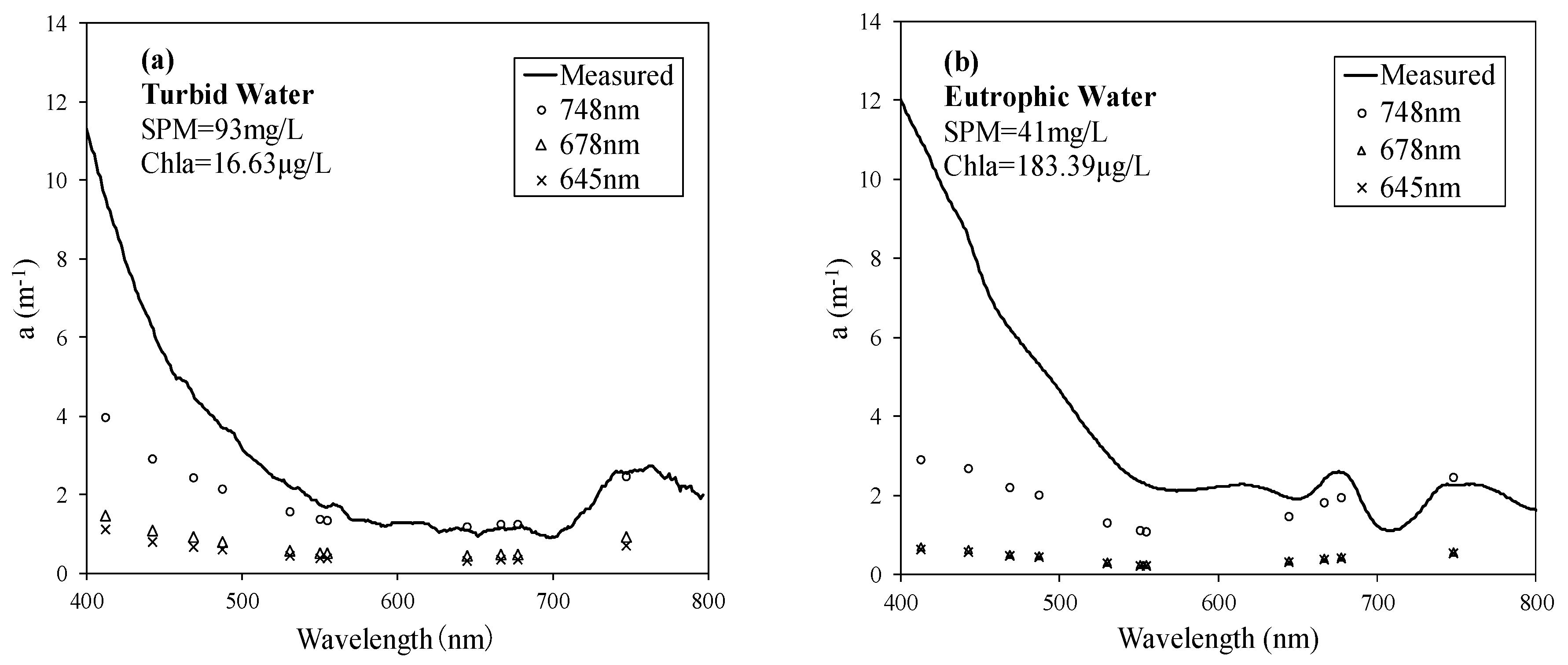
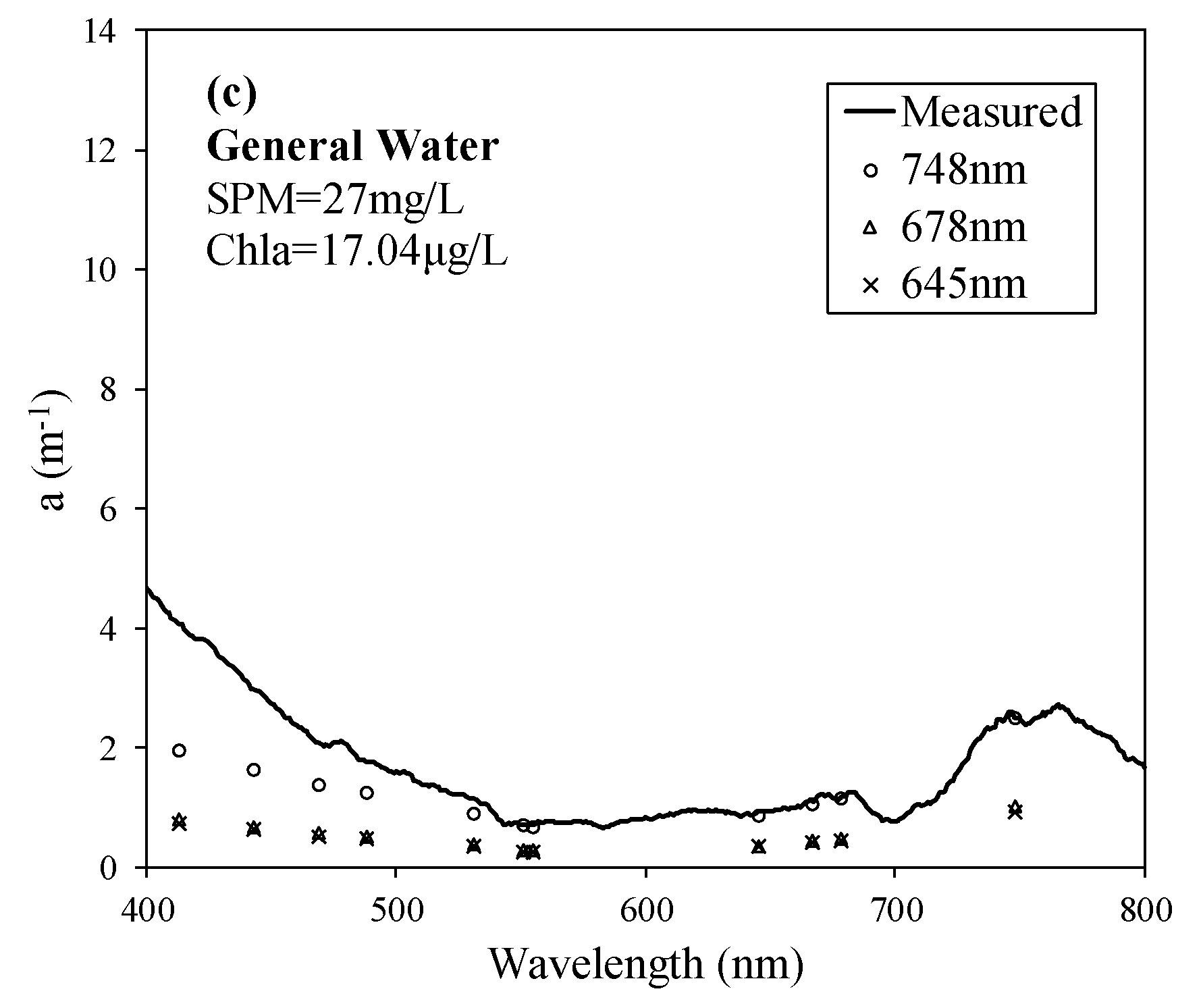
According to the basic water quality in Lake Chaohu, a_w increases and a_g and a_ph tend to decrease to 0 around 700 nm. Therefore, the reference wavelengths should be around 700 nm [43,44]. In our study, on the basis of the center wavelengths of MODIS bands, three reference wavelengths (645, 678, and 748 nm) were used to derive the total absorption coefficients of three different samples (Figure 3), which represent three kinds of water, namely, turbid, eutrophic, and general water. The turbid water has high SPM concentration (SPM concentration = 93 mg/L), the eutrophic water has high Chl a concentration (Chl a concentration = 183.39 μg/L) and the SPM and Chl a concentrations of general water are not high (SPM concentration = 27 mg/L, Chl a concentration = 17.04 μg/L). As the graphs suggest, in the case of using 748 nm as reference wavelength, the derived total absorption coefficients are much closer to the measured total absorption coefficients. We can conclude that, regardless of the type of water, setting 748 nm as the reference wavelength is most suitable for Lake Chaohu.

3.1.3. Model to Estimate the Power Value Y

Power value Y is a parameter used to estimate the backscattering coefficients at different wavelengths. If a(λ₀), u(λ₀), and backscattering coefficients of pure water at wavelength λ₀ (b_bw(λ₀)) are available, and the value of Y is estimated, then backscattering coefficients of particulate at wavelength λ₀ (b_bp(λ₀)) can be efficiently obtained. The values of total backscattering coefficient at wavelength λ (b_b(λ)) at all wavelengths are then derived. As shown in

Table 2. Power value Y of different types of waters.

Y	Areas	Methods	Reference
1.32–2.8	Lake Taihu	The initial value of Y is set to 0.1, and the step size is set to 0.1 for iteration, and then the data was used in calculation.	[15]
0.61–1.99	Huanghai Sea East China Sea	The backscattering coefficient is calculated based on measured data.	[45]
3.06	Lake Taihu	Measured data are used to calculate the backscattering coefficient.	[46]
1.3–3	Lake Kuncheng	The empirical model of the Y value is established by simulating the relationship between the reference Y value and reflectance ratio rrs(640)/rrs(715).	[17]

, different types of waters have different ranges of Y based on different reference wavelengths. A model to estimate the value of wavelength exponent Y in the case of Lake Chaohu should be established in this study.

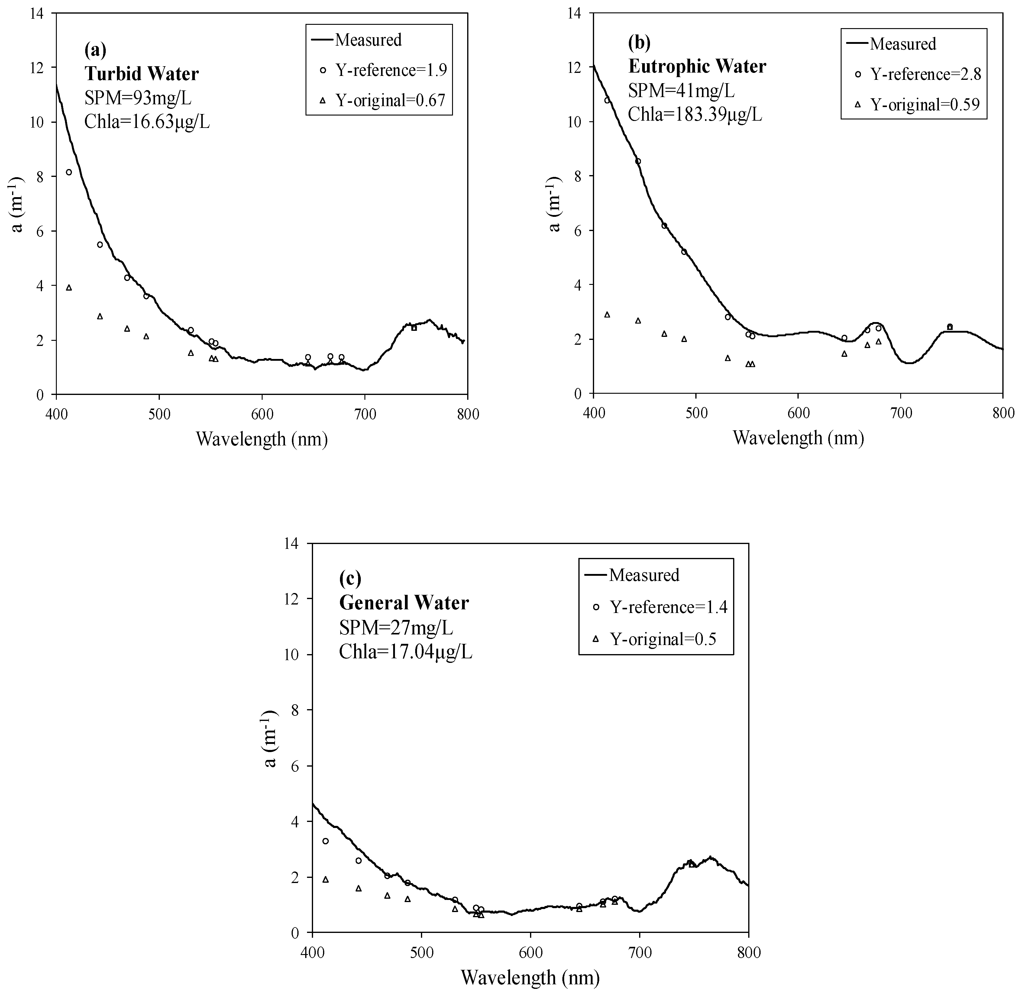
As no backscattering coefficient was measured in our research, the real Y value cannot be simulated by the original analytical model. Therefore, our research used the method of iteration [15]. We made Y iterate from 0.1 to 3 (step size of 0.1). When the minimum average absolute error (MAE) between the calculated total absorption coefficients and the measured total absorption coefficients at MODIS bands between 400 and 700 nm was less than 0.3, the best reference Y value of this sample was obtained. Figure 4 represents reference Y values of three different samples. The accuracy of the calculation results was greatly improved in the three cases mentioned.

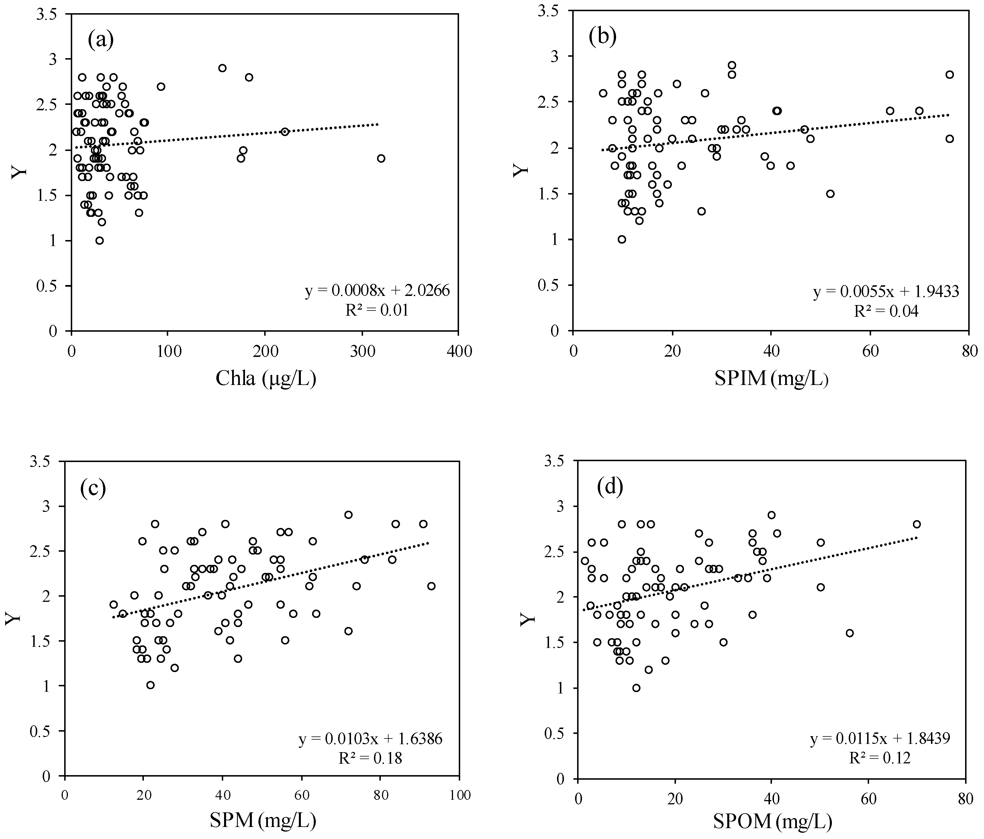
To obtain the reference Y value as accurately as possible, we had to establish a model for estimating Y. The Y value is related to parameters, such as R_rs, and concentrations of water compositions. First, we found out that a very good correlation did not exist between the ratio of R_rs and Y by applying measured data of Lake Chaohu. Thus, the relationships between the reference Y value and certain water quality parameters were established (Figure 5). As the graphs show, the relationship between SPM concentration and Y value had the best correlation. Therefore, this model (Y = 0.0103 * SPM + 1.6386) (N = 80) was used in our algorithm.

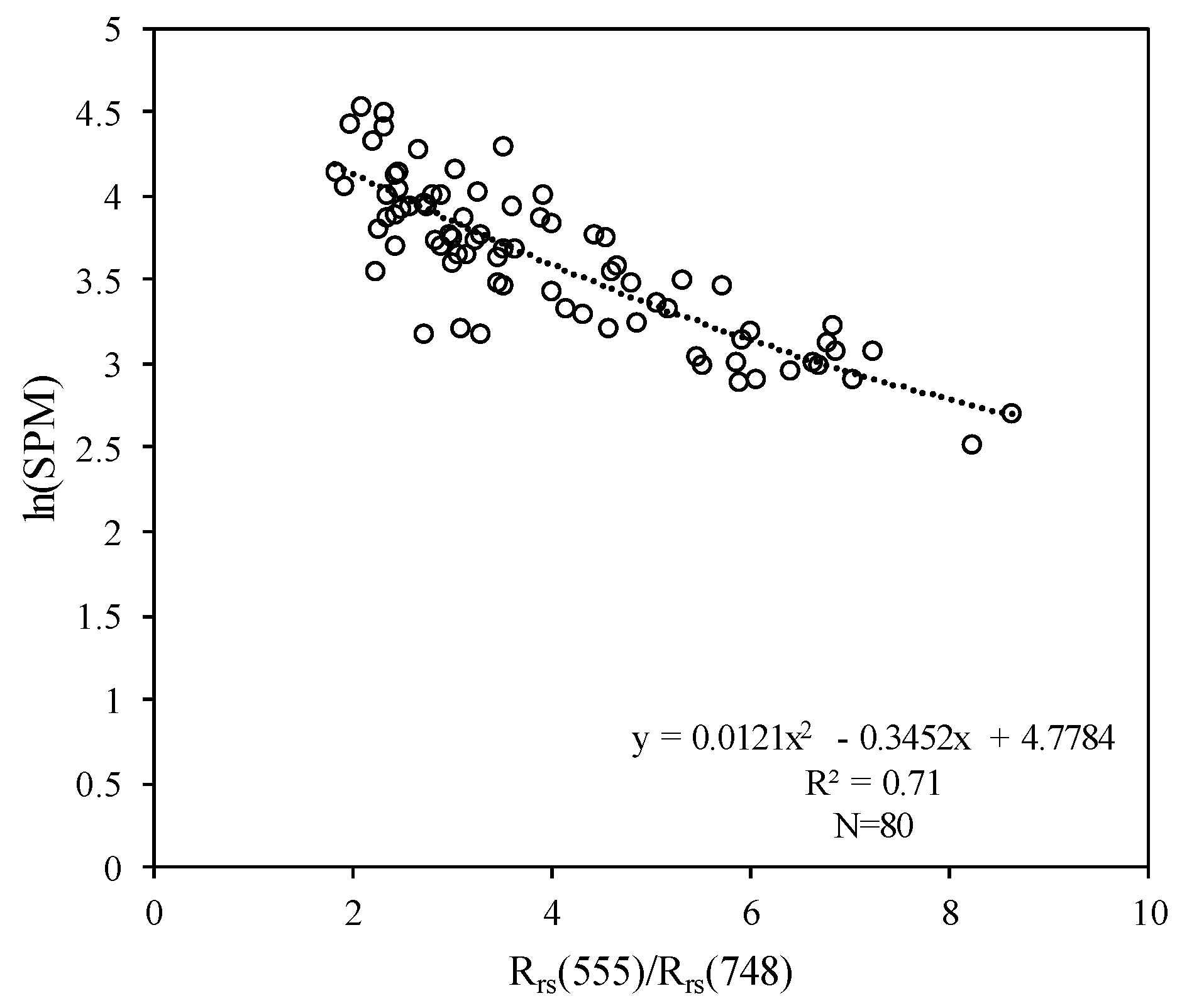
Even though the relationship between the Y value and SPM is modeled, water quality parameters cannot be determined from previous calculations. Thus, the model of SPM concentration and R_rs should be built. Based on several references, the general characteristics of SPM inversion algorithms are presented in

Table 3. General characteristics of SPM inversion algorithms.

Models	Areas	Reference
SPM = −1.91 + 1140.25 * Rrs(645)	Biloxi Bay	[47]
SPM = 9.65 * exp(58.81 * Rrs(645))	Lake Taihu	[48]
ln(SPM) = (Rrs(840)/Rrs(545) + 0.9614)/0.3193	Gironde	[49]
SPM = 349.83 * Rrs(645) + 2.9663	Muuga Port	[50]

. In this study, similar methods were used to construct the relationship between R_rs and SPM concentration. We found that SPM concentration and R_rs(555)/R_rs(748) had the best correlation (Figure 6).

3.2. Decomposition of Total Absorption Coefficient

Deriving a_ph(λ) and the absorption coefficients of gelbstoff and non-algal particulates (a_dg(λ)) from the total absorption coefficients (a(λ)) is a major challenge because the total absorption coefficient is the sum of a_w, a_ph, a_d, and a_g. Lee has developed an empirical algorithm for the separation [9]. We should estimate two parameters first: ζ, which is equal to a_ph(410)/a_ph(440), and ξ, which amounts to a_dg(410)/a_dg(440). The value of ζ is obtained using the ratio of measured r_rs(440)/r_rs(555) data in the QAA algorithm.

3.2.1. The Value of Spectral Slope of a_dg Spectrum (S)

The spectral slope of a_dg spectrum (S) can depict the spectral shape of a_dg(λ), which is the sum of a_g(λ) and a_d(λ). In the original QAA process, S was valued at 0.015 nm⁻¹. The measured data of a_dg(410) and a_dg(440) in Lake Chaohu were used to calculate S. We concluded that the average value of S is 0.01453, and the standard deviation is 0.001129, which means that all the values are basically distributed around the average. Therefore, we selected the mean, 0.01453, as the value of S in our study.

3.2.2. The Relationship of a_ph and r_rs

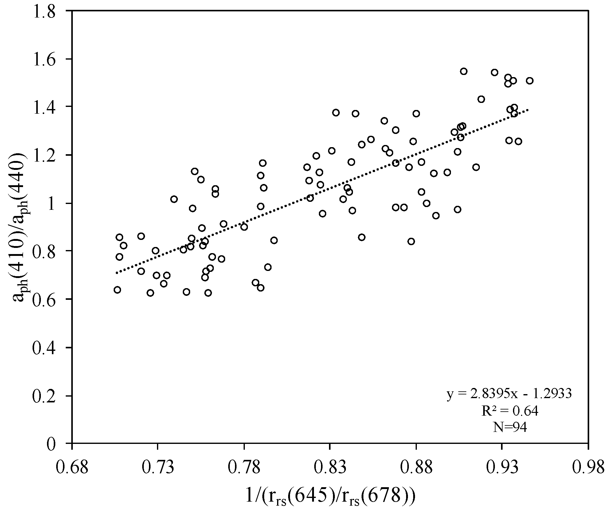
The value of a_ph(410)/a_ph(440) is calculated from the ratio of r_rs(440)/r_rs(555) through an empirical formula in the original QAA algorithm [9]. Considering the research area, we had to rebuild the relationship between a_ph and r_rs by simulating the relationship between the a_ph(410)/a_ph(440) and the spectral ratio r_rs of the center wavelengths of MODIS bands between 400 and 800 nm. The model was constructed using r_rs(645)/r_rs(678) with a high correlation, as shown in Figure 7.

The specific calculation process of this improved QAA is as follows (

Table 4. Steps of the improved quasi-analytical algorithm (QAA).

Step	Formula	Approach
0	$r_{rs}=R_{rs}/\left(0.52+1.7R_{rs}\right)$	Semi-analytical
1	$u\left(\lambda \right)=\frac{-g_0+{[{(g_0)}^2+4g_1{r}_{rs}\left(\lambda \right)]}^{1/2}}{2g_1}$	Semi-analytical
2	$\mathrm{a}\left(748\right)=a_w\left(748\right)$	Empirical
3	$b_{bp}\left(748\right)=\frac{u\left(748\right)a\left(748\right)}{1-u\left(748\right)}-b_{bw}\left(748\right)$	Analytical
4	$\mathrm{Y}=0.0103*\exp [0.0121{(R_{rs}\left(555\right)/R_{rs}\left(748\right))}^2-0.3452(R_{rs}\left(555\right)/R_{rs}\left(748\right))+4.7784]+1.6386$	Empirical
5	$b_{bp}\left(\lambda \right)=b_{bp}\left(748\right){\left(\frac{748}{\lambda }\right)}^Y$	Semi-analytical
6	$\mathrm{a}\left(\lambda \right)=\frac{\left[1-u\left(\lambda \right)\right]\left[b_{bw}\left(\lambda \right)+b_{bp}\left(\lambda \right)\right]}{u\left(\lambda \right)}$	Analytical
7	$\mathsf{\zeta }=\frac{a_{ph}\left(410\right)}{a_{ph}\left(440\right)}=\frac{2.8395}{r_{rs}\left(645\right)/r_{rs}\left(678\right)}-1.2933$	Empirical
8	$\mathsf{\xi }=\frac{a_{dg}\left(410\right)}{a_{dg}\left(440\right)}=\exp \left[S\left(440-410\right)\right]$	Semi-analytical
9	$a_{dg}\left(440\right)=\frac{a\left(410\right)-\mathsf{\zeta }\mathrm{a}\left(440\right)}{\mathsf{\xi }-\mathsf{\zeta }}-\frac{a_w\left(410\right)-\mathsf{\zeta }{a}_w\left(440\right)}{\mathsf{\xi }-\mathsf{\zeta }}$	Analytical
10	$a_{ph}\left(440\right)=a\left(440\right)-a_{dg}\left(440\right)-a_w\left(440\right)$	Analytical

).

To evaluate the performance of this algorithm and the accuracy of the MOD09 data after correction, three parameters were calculated.

The accuracy evaluation indicators used in this study include average relative error (MRE) [51], average absolute error (MAE) and root mean square error (RMSE) [52]. The expression equations are as follows:

$$\mathrm{MRE}=\frac{1}{N}{{\displaystyle \sum }}_{i=1}^N\left|\frac{y_i-x_i}{x_i}\right|$$

(4)

$$\mathrm{MAE}=\frac{1}{N}{{\displaystyle \sum }}_{i=1}^N\left|y_i-x_i\right|$$

(5)

$$\mathrm{RMSE}=\sqrt{\frac{1}{N}{{\displaystyle \sum }}_{i=1}^N{\left(y_i-x_i\right)}^2}$$

(6)

where x represents the measured value, y represents the derived value, and N represents the number of samples. Coefficient of determination (R²) was also used to assess the accuracy of the model.

4. Results and Validation

4.1. MODIS Corrected Data Accuracy Evaluation

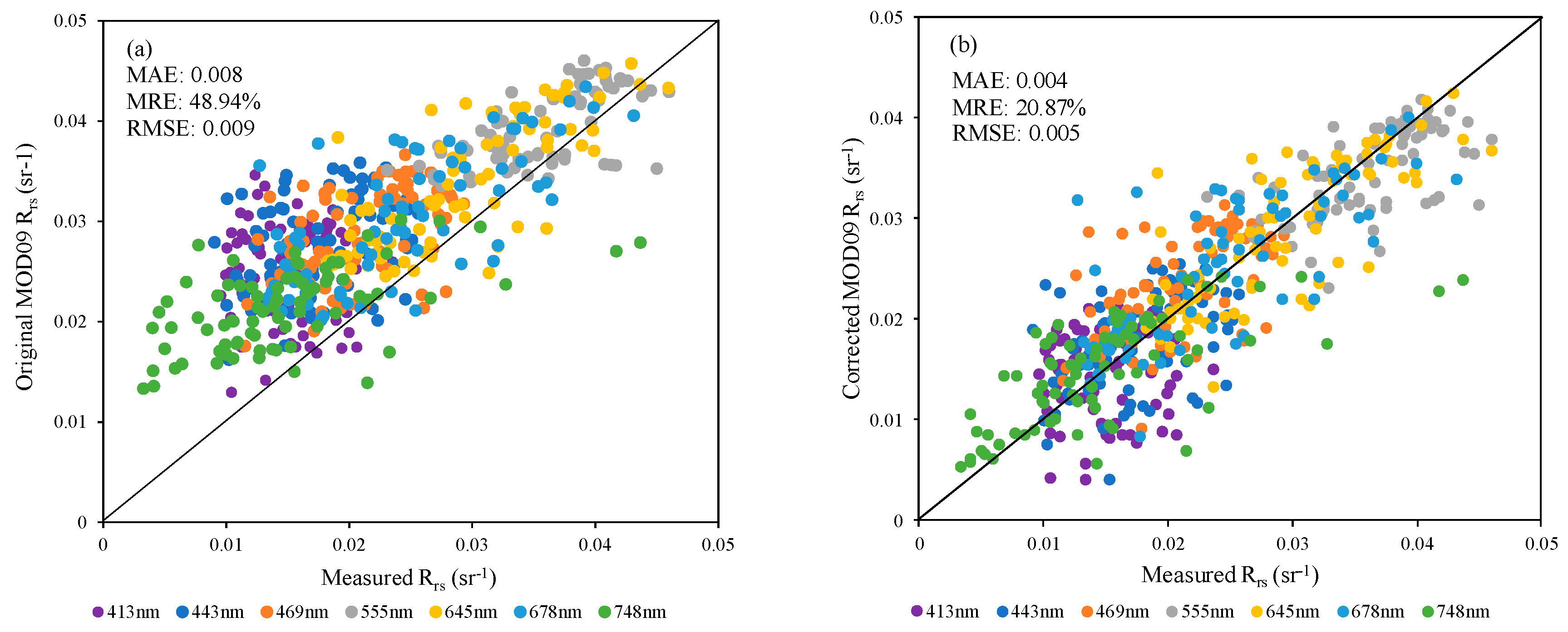
Compared with the measured R_rs data, the errors of the R_rs derived from MOD09 product were evaluated in this paper. Before correction, as shown in Figure 8a, most of the 79 points of R_rs were above the 1:1 line, indicating that, on the same scale, the data at 413, 443, 469, 555, 645, 678, and 748 nm were generally larger than the measured data; after using this correction method, as shown in Figure 8b, the R_rs of the points generally had a good linear correlation. The scatterplots were mostly distributed near the 1:1 line. At the wavelength 748 nm, the corrected values were still a little higher than the measured data.

Table 5. Error statistics of R_rs derived from the original MOD09.

Wavelength (nm)	MRE (%)	RMSE (sr−1)
413	76.46	0.012
443	68.35	0.012
555	13.83	0.005
645	21.24	0.006
678	34.95	0.008
748	84.66	0.009

and

Table 6. Error statistics of R_rs derived from the corrected MOD09.

Wavelength (nm)	MRE (%)	RMSE (sr−1)
413	30.02	0.005
443	24.15	0.005
555	9.23	0.004
645	11.50	0.005
678	17.51	0.005
748	31.23	0.006

show the statistics of the errors before and after correction. The MRE at 413 nm was reduced from 76.46% to 30.02%, and the RMSE was from 0.012 sr⁻¹ to 0.005 sr⁻¹. The MRE value before correction at the 555-nm band was 13.83%, while the MRE value after correction was only 9.23%. The MRE of 748 nm before correction was as high as 84.66%, while the MRE after correction was 31.23%, and the RMSE also decreased from 0.009 sr⁻¹ to 0.006 sr⁻¹. Compared with the original MOD09, the RMSEs and MREs of the corrected MOD09 at all bands were significantly reduced. This shows that the correction method we used in this study can obtain more accurate R_rs.

4.2. Inversion of Absorption Coefficients in Different Water Types

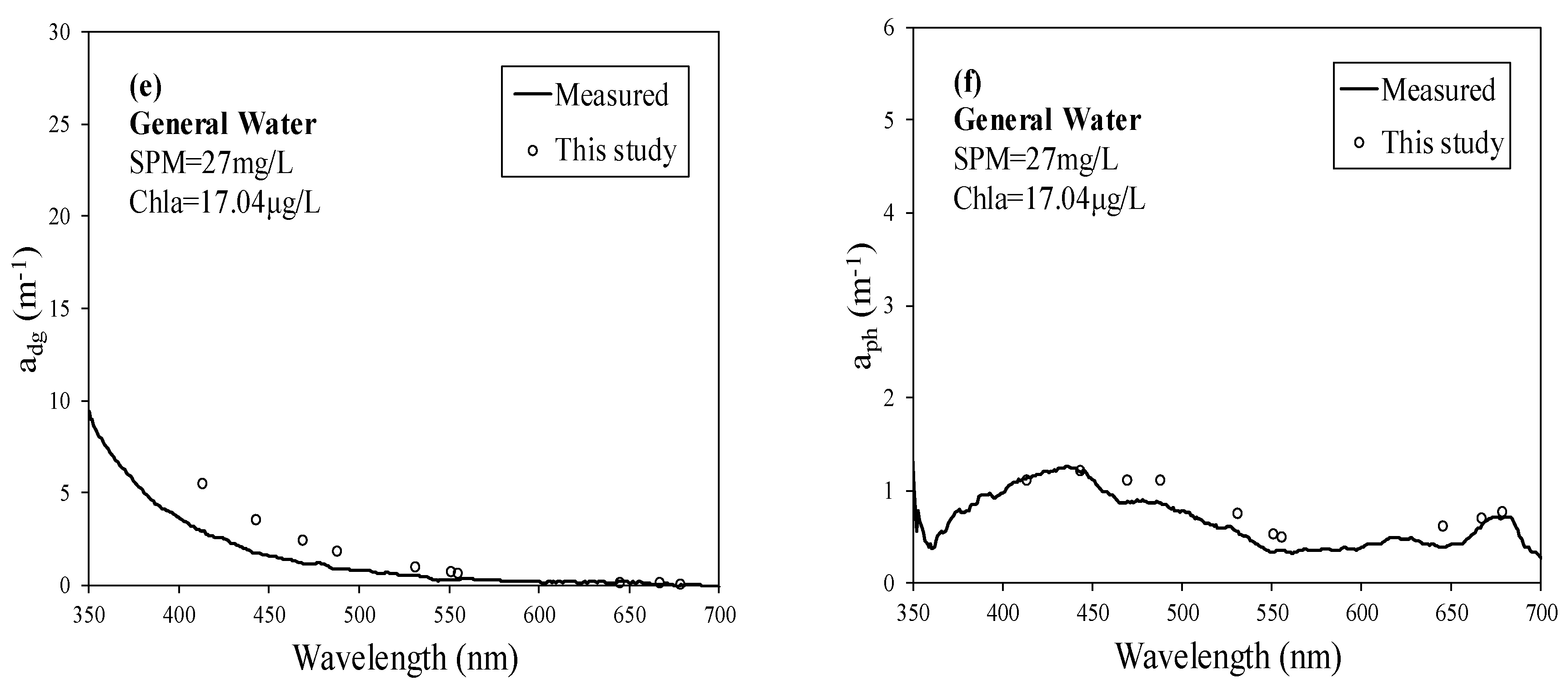
The measured data of R_rs of Lake Chaohu were applied to this model to obtain absorption coefficients. The wavelengths of input R_rs were at center wavelengths of MODIS bands between 400 and 700 nm, including 413, 443, 469, 488, 531, 551, 555, 645, 667, and 678 nm. The retrieved IOPs included a_ph(λ) and a_dg(λ) of these wavelengths. Figure 9 shows the comparison of retrieved and measured a_ph and a_dg of the three different types of water. The concentrations of SPM and Chl a are shown in the graphs.

As shown in Figure 9, this model tends to be more suitable for general waters as it is more effective in obtaining a_ph when applied to general water than eutrophic water. The values of obtained a_dg are closer to those of measured a_dg than a_ph. Thus, the accuracy of derived a_ph in all water conditions needs to be improved especially in the case of turbid waters.

4.3. Derived Values at Typical Wavelengths

To present a general description of the performance of this algorithm, we used 25 field-measured test samples to derive a(λ), a_ph(λ), and a_dg(λ) at 410 nm, 440 nm, and center wavelengths of MODIS bands between 400 and 700 nm, then compared them with measured data.

Table 7. Evaluation of the errors between measured and derived values.

Values	MRE (%)	RMSE (sr−1)
a(λ)	18.96	0.88
aph(λ)	102.04	0.52
adg(λ)	30.33	1.09

, Figure 10 and Figure 11 show the results of this analysis.

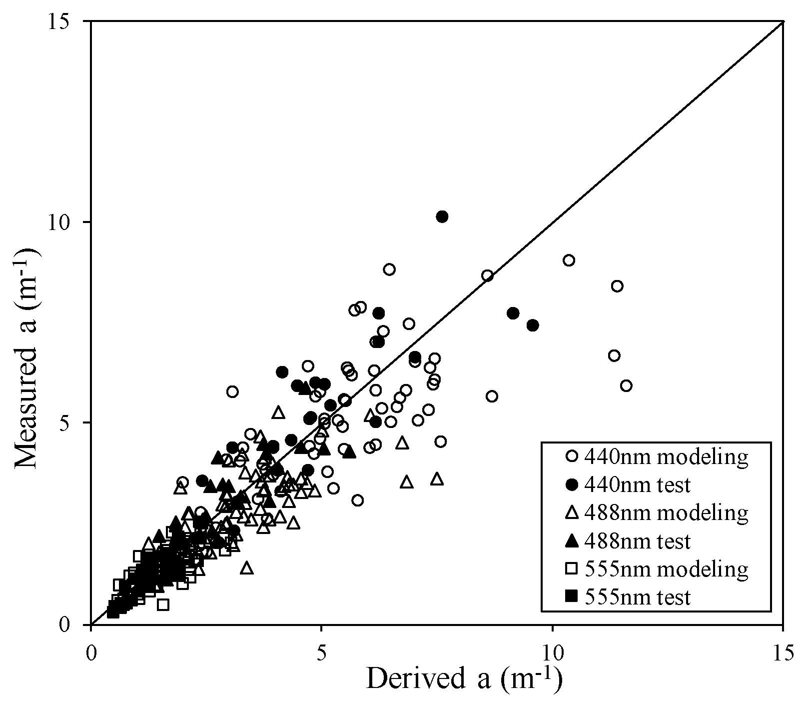
Figure 10 shows the total absorption coefficients of typical wavelengths such as 440, 488, and 555 nm.

For these wavelengths, the MRE values of test data were 17.68%, 19.10%, and 18.71%, and R² values were 0.74, 0.75, and 0.88, which indicate a good correlation at the aforementioned wavelengths (Figure 10). Some points were distributed below the 1:1 line, which shows that the derived total absorption coefficients were slightly higher than the measured total absorption coefficients. It was due to the errors between the estimated values of Y and the reference values of Y varying at different conditions. The selection of a reference wavelength may also have had some impact on this situation. Additionally, the errors in measurement of field data can also be responsible for the observed differences. As a result, the accuracy of this model to derive total absorption coefficients needs improvement in these aspects.

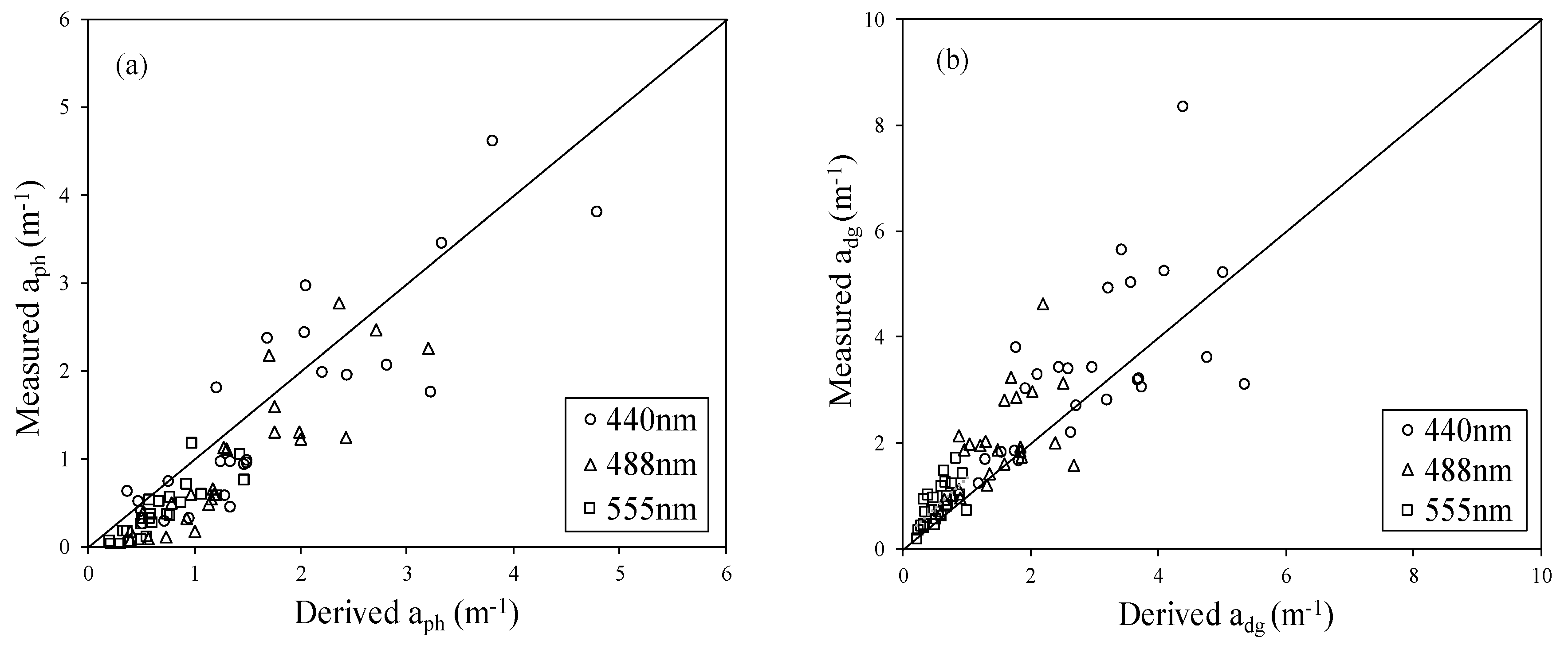
The MRE values of derived a_ph at 440, 488, and 555 nm were 55.08%, 126.59%, and 184.72%, and the R² values were 0.76, 0.78, and 0.72, while the MRE values of a_dg were 24.64%, 27.52%, and 32.20% and the R² values were 0.38, 0.36, and 0.43 (Figure 11). Comparison and analysis showed that the derived a_dg were moderately smaller than the measured values, but more errors were found at the retrieval of a_ph. When we compared the inversion of a_ph at three wavelengths, we easily concluded that the MREs of values at longer wavelengths were bigger than those at shorter wavelengths. The derived a_ph were mostly distributed below the 1:1 line, which means that the calculated values were larger than the measured values. Gelbstoff and detritus contribute substantially to the total absorption coefficients at 410 and 440 nm. In the direct decomposition of total a(λ) to a_ph(λ) and a_dg(λ), values of ζ and ξ were estimated. The errors in these sectors were transferred to the estimated values of a_dg(440), which then influenced the final inversion of this model. Thus, different wavelengths can be used in future studies to improve the accuracy of decomposition of total absorption coefficients. As this test included a limited range of water samples, it cannot represent the accuracy completely. Further detailed tests with measured data are desired and needed to improve this model to derive a_ph and a_dg optimally.

5. Discussion

5.1. Error Propagation

Error propagation means errors that may occur at each step have varying effects on the analysis results. The errors in each step propagate to the next step in the step-by-step process. We analyzed the error propagation of some steps of this algorithm by using modeling data (

Table 8. Error propagation of steps of the improved QAA.

Step	Formulas	Approach	Relative Errors Range	MRE	RMSE (sr−1)
2	$\mathrm{a}\left(748\right)=a_w\left(748\right)$	Empirical	−14.26% ~12.61%	3.68%	0.12
4	$\mathrm{Y}=0.0103*\exp [0.0121{(R_{rs}\left(555\right)/R_{rs}\left(748\right))}^2-0.3452(R_{rs}\left(555\right)/R_{rs}\left(748\right))+4.7784]+1.6386$	Empirical	−34.14% ~129.31%	19.31%	0.72
a				26.36%	1.09
7	$\mathsf{\zeta }=\frac{a_{p\mathrm{h}}\left(410\right)}{a_{p\mathrm{h}}\left(440\right)}=\frac{2.8395}{r_{rs}\left(645\right)/r_{rs}\left(678\right)}-1.2933$	Empirical	−25.91% 46.19%	12.62%	0.15
8	$\mathsf{\xi }=\frac{a_{dg}\left(410\right)}{a_{dg}\left(440\right)}=\exp \left[S\left(440-410\right)\right]$	Semi-analytical	−8.19% ~8.12%	2.74%	0.05
adg440				28.25%	1.50
adg				35.07%	1.22
aph				133.10%	1.07

). This part shows the performance assessment of absorption coefficients at wavelengths 410, 440 nm, and the center wavelengths of MODIS bands between 400 and 700 nm.

As the table suggests, all the errors were from the empirical and semi-analytical algorithms. Through the steps to retrieve the total absorption coefficients, the MRE between calculated Y values and reference Y values was approximately 19.31%, which was due to the relationship of R_rs, SPM concentration, and the value of Y. Therefore, this step consequently led to the errors of the calculated total absorption. The retrieval of a_ph(410)/a_ph(440) and a_dg(410)/a_dg(440) had errors of 12.62% and 2.74%, respectively, which showed that the main source of the errors of a_dg was due to the calculation of a_dg(440) and then extended to a_dg in the full wavelength range. Also, the errors of derived total absorption coefficients affected the accuracy of a_ph and a_dg. At the same time, because the values of measured a_ph at longer wavelengths and some samples were small, the MREs increased, thereby influencing the total MRE of a_ph.

5.2. Comparison with QAA

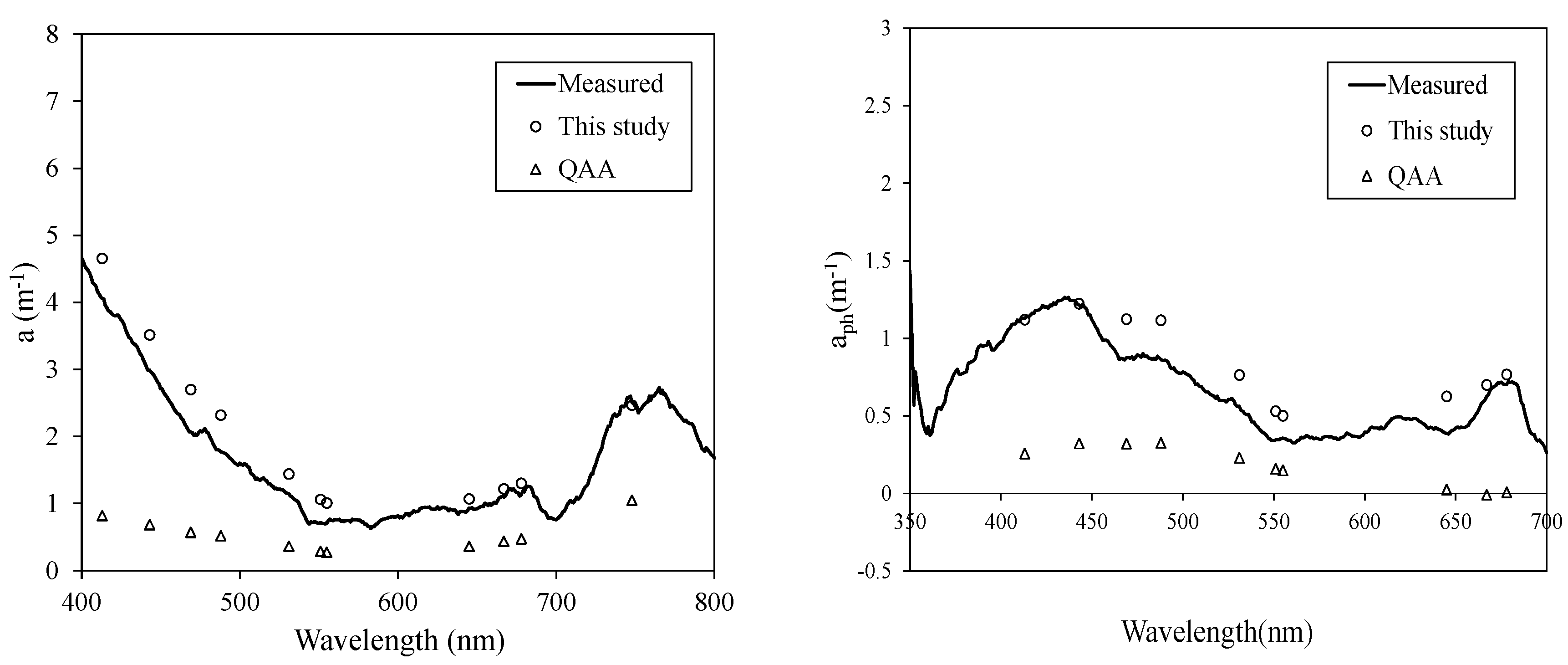
As mentioned, QAA did not function well when applied to Lake Chaohu (Figure 12). In the case below, especially at a wavelength longer than 600 nm, the values of a_ph are almost less than zero, which was impossible for Lake Chaohu. Therefore, improving this algorithm is necessary.

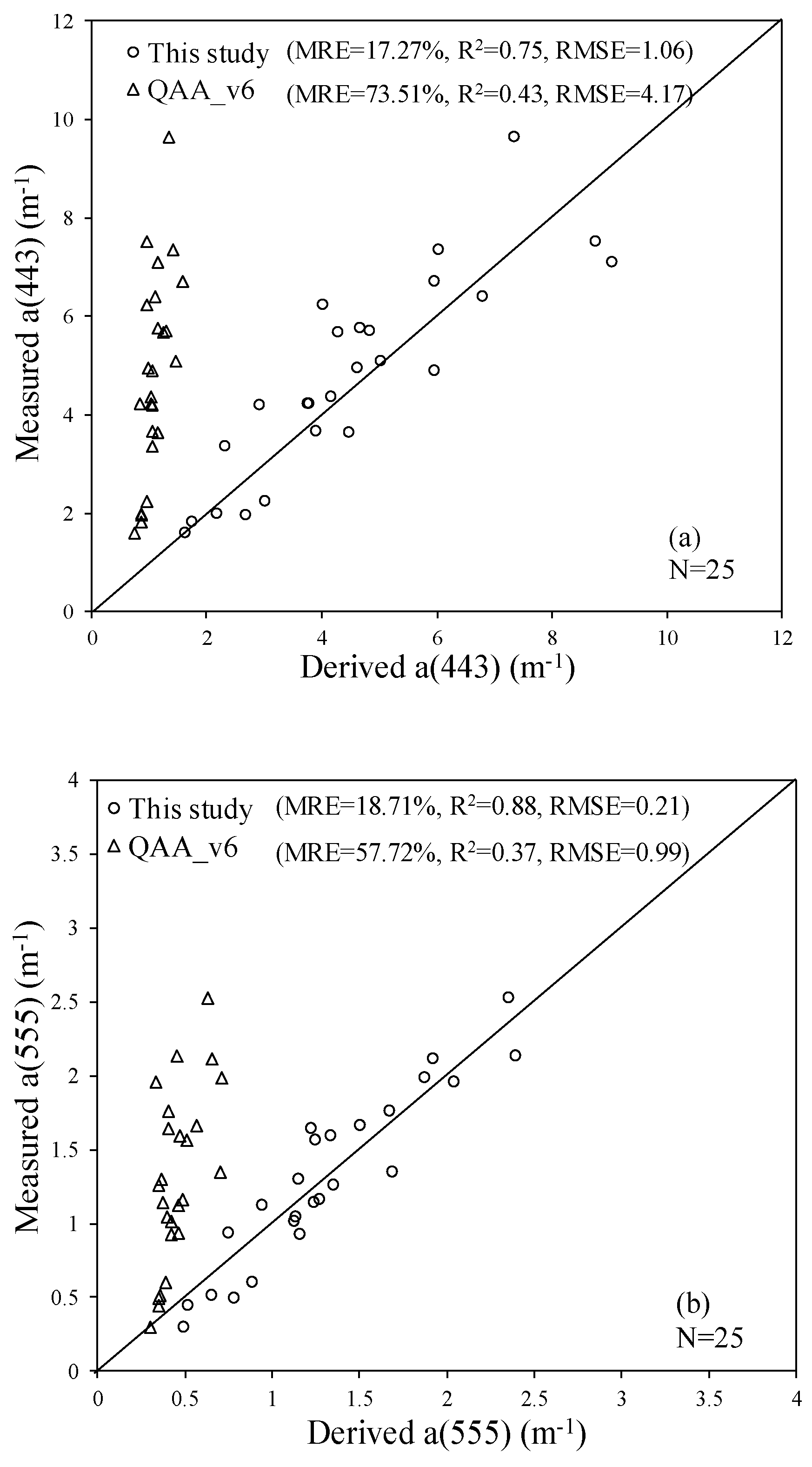
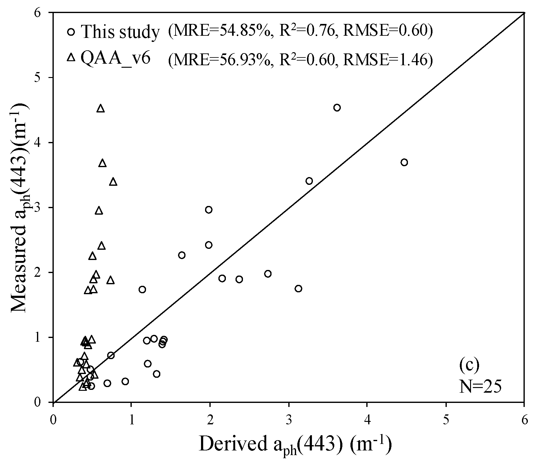
The algorithm in this article was further validated by the measured dataset collected in Lake Chaohu. The version, QAA_v6, tended to be more suitable for turbid coastal waters, so it was also applied to the same dataset (Figure 13). The assessment results for retrieved absorption coefficients at some special wavelengths are summarized in

Table 9. Accuracy assessment of the algorithm in this study and QAA_v6.

	Algorithms	N	MRE	R2	RMSE (sr−1)
a(443)	this study	25	17.27%	0.75	1.06
	QAA_v6	25	73.51%	0.43	4.17
a(555)	this study	25	18.71%	0.88	0.21
	QAA_v6	25	57.72%	0.37	0.99
aph(443)	this study	25	54.85%	0.76	0.60
	QAA_v6	25	56.93%	0.60	1.46

. The RMSEs and MREs for the algorithm in this study were in the range of 0.21–1.06 sr⁻¹ and 17.27–54.85%, while those of QAA_v6 were 0.99–4.17 sr⁻¹ and 56.93–73.51%, respectively. Specifically, the RMSEs and MREs of the QAA_v6 were larger than those of the algorithm in this study. The values of total absorption coefficients derived from QAA_v6 were much smaller than measured data. The larger RMSEs’ and MREs’ values derived from QAA_v6 were mainly because of a short reference wavelength and inappropriate estimated formulas that do not work for turbid Case 2 waters. The a_ph(443) was also retrieved based on QAA_v6 for comparison. Scatterplots of derived and measured a_ph(443) are shown in Figure 13, and the evaluation indices are also demonstrated in Table 9. In general, we can conclude that the algorithm in this research had smaller errors of RMSE and MRE of 0.60 sr⁻¹ and 54.85%, respectively, compared with those of 1.46 sr⁻¹ and 56.93% from the a_ph(443) estimated by QAA_v6. However, because the a_ph derived from the algorithm in this study tended to be larger than measured data, at some points, a_ph(443) derived from QAA-v6 were closer to measured data than those of this study.

5.3. MODIS Data Inversion

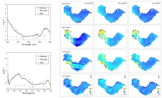
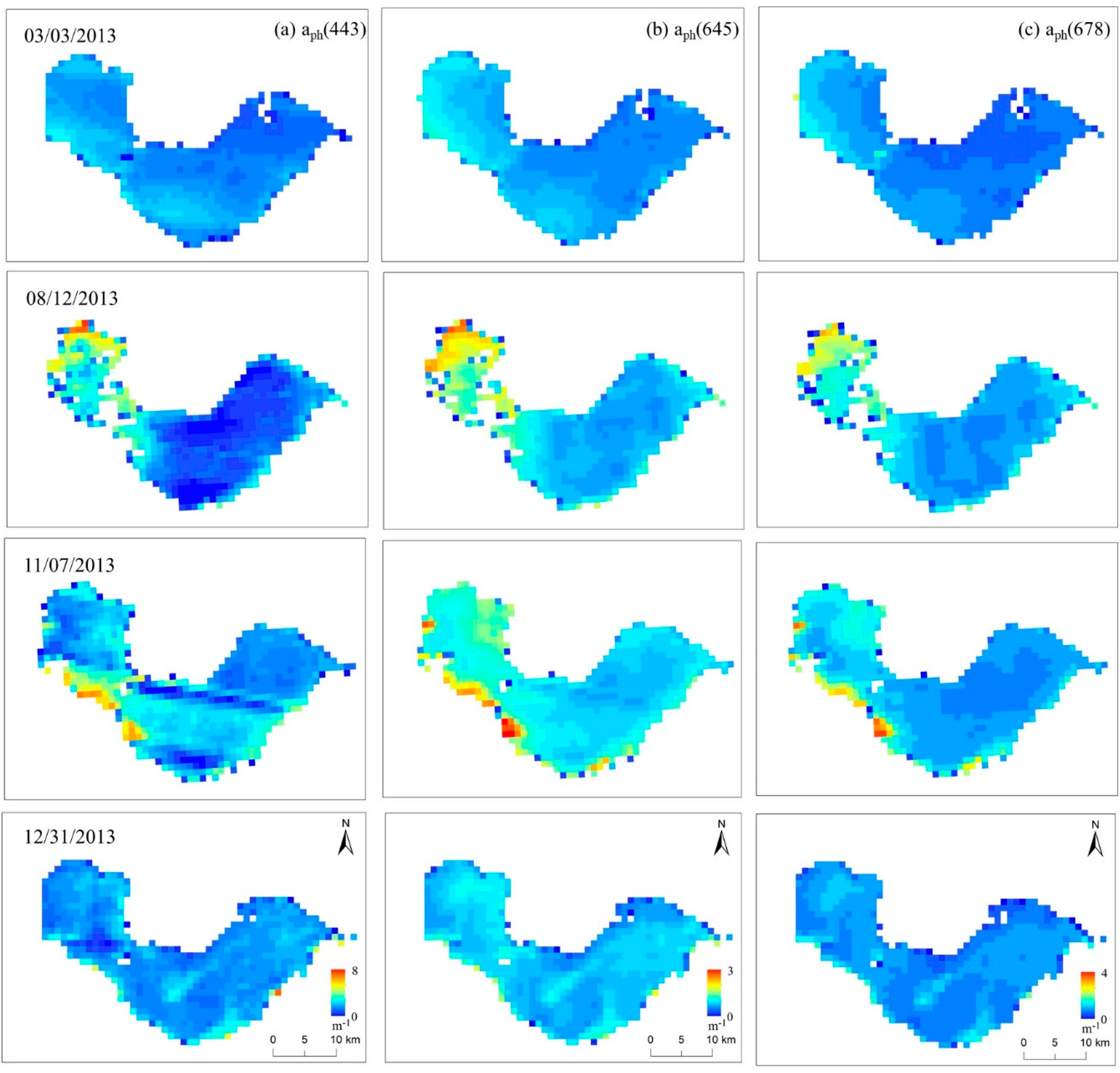
We used the algorithm proposed in this study to calculate the a_ph at 443, 645, and 678 nm of Lake Chaohu in 2013 by applying corrected MOD09 data (Figure 14). Because of the difference of bands, we used MODIS bands 8 and 9 data to be the input parameters at 410 and 440 nm. The missing parts of the image were due to saturation that usually occurs at long wavelengths of 1-km resolution of this product. Even though there were some problems with this product, we still could verify the general seasonal changes of Lake Chaohu. Generally, a_ph varied largely in Lake Chaohu. High a_ph was observed in the northwestern parts of Lake Chaohu in the summer and autumn, and a_ph were relatively lower in the spring and winter. This pattern is consistent with the known phenomenon. Cyanobacteria blooms occur mainly in the western area in the summer, and the large amount of cyanobacteria in the western part is due to the exogenous load of the lakes mainly from the northwest of the basin. The suitable temperature of 20–34 ℃ in summer, the higher N and P concentrations, the higher PH value, the appropriate light intensity, and other environmental conditions provide the perfect environment for the growth of cyanobacteria. Therefore, a_ph tends to be higher in the western part in summer.

6. Conclusions

Based on the field-measured data of Lake Chaohu, this study improved the QAA algorithm to provide an effective inversion of the IOPs of Lake Chaohu according to MODIS bands. The appropriate reference wavelength was shifted to 748 nm according to the measured data from the lake, and the applicable empirical model of the Y value was established by building models with SPM concentration and R_rs. The a_dg and a_ph were also derived by changing important parameters according to Lake Chaohu. To test the accuracy of this model, we applied this algorithm to a test dataset. This algorithm tends to be more suitable for general waters. It works better in the retrieval of total absorption coefficients in the condition of Lake Chaohu than original QAA and QAA_v6 do. The derived a_dg of this algorithm tend to be smaller than measured data and the derived a_ph tend to be bigger than measured values at some points. We also used the corrected MOD09 data to calculate a_ph at 443, 645, and 678 nm by the model proposed in this study. It shows that, in summer and autumn, a_ph tend to be higher in the northwestern part of Lake Chaohu, which is similar to the previous studies.

More independent tests with field measurement are required for validating and improving the algorithm. This algorithm needs to be improved in several aspects. First, the accuracy of the empirical model for calculating the Y value can be developed because it is one of the errors of the derived total absorption coefficients. Secondly, basic wavelengths can be changed to derive accurate a_ph and a_dg. Combining the measured backscattering coefficients with the derived backscattering coefficients in future research will help improve the accuracy of this algorithm.

References

- Mobley, C.D. Light and Water: Radiative Transfer in Natural Waters; Academic Press: Cambridge, MA, USA, 1994. [Google Scholar]
- Ma, R.; Tang, J.; Dai, J. Bio-optical model with optimal parameter suitable for Taihu Lake in water colour remote sensing. Int. J. Remote Sens. 2006, 27, 4305–4328. [Google Scholar] [CrossRef]
- Carder, K.; Chen, F.; Cannizzaro, J.; Campbell, J.; Mitchell, B. Performance of the MODIS semi-analytical ocean color algorithm for chlorophyll-a. Adv. Space Res. 2004, 33, 1152–1159. [Google Scholar] [CrossRef]
- Gons, H.J. Optical teledetection of chlorophyll a in turbid inland waters. Environ. Sci. Technol. 1999, 33, 1127–1132. [Google Scholar] [CrossRef]
- Carder, K.L.; Chen, F.; Lee, Z.; Hawes, S.; Kamykowski, D. Semianalytic Moderate-Resolution Imaging Spectrometer algorithms for chlorophyll a and absorption with bio-optical domains based on nitrate-depletion temperatures. J. Geophys. Res. Oceans 1999, 104, 5403–5421. [Google Scholar] [CrossRef]
- Hoge, F.E.; Lyon, P.E. Satellite retrieval of inherent optical properties by linear matrix inversion of oceanic radiance models: An analysis of model and radiance measurement errors. J. Geophys. Res. Oceans 1996, 101, 16631–16648. [Google Scholar] [CrossRef]
- Hoge, F.E.; Lyon, P.E. Spectral parameters of inherent optical property models: Method for satellite retrieval by matrix inversion of an oceanic radiance model. Appl. Opt. 1999, 38, 1657–1662. [Google Scholar] [CrossRef]
- Doerffer, R.; Helmut, S. Neural network for retrieval of concentrations of water constituents with the possibility of detecting exceptional out of scope spectra. In Proceedings of the IGARSS 2000. IEEE 2000 International Geoscience and Remote Sensing Symposium. Taking the Pulse of the Planet: The Role of Remote Sensing in Managing the Environment Proceedings, Piscataway, NJ, USA, 24–28 July 2000; pp. 714–717. [Google Scholar]
- Lee, Z.; Carder, K.L.; Arnone, R.A. Deriving inherent optical properties from water color: A multiband quasi-analytical algorithm for optically deep waters. Appl. Opt. 2002, 41, 5755–5772. [Google Scholar] [CrossRef]
- Lee, Z.; Lubac, B.; Werdell, J. Update of the Quasi-Analytical Algorithm (QAA_v6) [R/OL]. Available online: http://www.ioccg.org/groups/Software_OCA/QAA_v6_2014209.pdf (accessed on 1 November 2014).
- Hu, L.-B.; Liu, Z.-S. Deriving Absorption Coefficients from Remote Sensing Reflectance Using the Quasi-Analytical Algorithm (QAA) in the Yellow Sea. Period. Ocean Univ. China 2007, S2, 154–160. [Google Scholar]
- Wang, W.-Q.; Dong, -Q.; Shang, S.-L.; Wu, J.-Y.; Lee, Z.-P. An evaluation of two semi-analytical ocean color algorithms for waters of the South China Sea. J. Trop. Oceanogr. 2009, 28, 35–42. [Google Scholar]
- Hao, Y.-L.; Cao, W.-X.; Cui, T.-W.; Zhang, J. The retrieval of oceanic inherent optical properties based on semianalytical algorithm during the red ride. Acta Oceanol. Sin. 2011, 33, 52–65. [Google Scholar]
- Gordon, H.; More, A. Remote assessment of ocean color for interpretation of satellite visible imagery, a review. In Lecture Notes on Coastal and Estuarine Studies; Barber, R.T., Mooers, C.N.K., Bowman, M.J., Zeitschel, B., Eds.; Springer: New York, NY, USA, 1983. [Google Scholar]
- Le, C.-F.; Li, Y.-M.; Zha, Y.; Sun, D.-Y.; Lu, H. Simulation of backscattering properties of Taihu Lake. Adv. Water Sci. 2009, 20, 707–713. [Google Scholar]
- Le, C.-F.; Li, Y.-M.; Zha, Y.; Sun, D.; Yin, B. Validation of a quasi-analytical algorithm for highly turbid eutrophic water of Meiliang Bay in Taihu Lake, China. IEEE Trans. Geosci. Remote Sens. 2009, 47, 2492–2500. [Google Scholar]
- Xie, F.; Guo, Z.; Tian, Y.; Liu, C.; Lei, X. Retrieving Inherent Optical Properties of Lake Kuncheng based on Quasi-Analytical Algorithm. Remote Sens. Technol. Appl. 2015, 30, 242–250. [Google Scholar]
- Jiang, L.; Zhao, D.; Wang, L.; Wang, X. Methods and Research Progress on Backscattering Coefficient in the Water. Remote Sens. Technol. Appl. 2013, 28, 150–156. [Google Scholar]
- Wei, Y.; Matsushita, B.; Jin, C.; Yoshimura, K.; Fukushima, T. Retrieval of Inherent Optical Properties for Turbid Inland Waters from Remote-Sensing Reflectance. IEEE Trans. Geosci. Remote Sens. 2013, 51, 3761–3773. [Google Scholar]
- Li, S.; Song, K.; Mu, G.; Ying, Z.; Ren, J. Evaluation of the Quasi-Analytical Algorithm (QAA) for Estimating Total Absorption Coefficient of Turbid Inland Waters in Northeast China. IEEE J. Sel. Top. Appl. Earth Obs. Remote Sens. 2016, 9, 4022–4036. [Google Scholar] [CrossRef]
- Chen, X.; Yang, X.; Dong, X.; Liu, E. Environmental changes in Chaohu Lake (southeast, China) since the mid 20th century: The interactive impacts of nutrients, hydrology and climate. Limnol. Ecol. Manag. Inland Waters 2013, 43, 10–17. [Google Scholar] [CrossRef]
- Tu, Q.; Gu, D.; Yi, C.; Xu, Z.; Han, G. The Researches on the Lake Chaohu Eutrophication; Publisher of University of Science and Technology of China: Hefei, China, 1990. [Google Scholar]
- Qin, N.; He, W.; Kong, X.-Z.; Liu, W.-X.; He, Q.-S.; Yang, B.; Ouyang, H.-L.; Wang, Q.-M.; Xu, F.-L. Atmospheric partitioning and the air–water exchange of polycyclic aromatic hydrocarbons in a large shallow Chinese lake (Lake Chaohu). Chemosphere 2013, 93, 1685–1693. [Google Scholar] [CrossRef]
- Yang, L.; Lei, K.; Meng, W.; Fu, G.; Yan, W. Temporal and spatial changes in nutrients and chlorophyll-α in a shallow lake, Lake Chaohu, China: An 11-year investigation. J. Environ. Sci. 2013, 25, 1117–1123. [Google Scholar] [CrossRef]
- Jiang, Y.-J.; He, W.; Liu, W.-X.; Qin, N.; Ouyang, H.-L.; Wang, Q.-M.; Kong, X.-Z.; He, Q.-S.; Yang, C.; Yang, B. The seasonal and spatial variations of phytoplankton community and their correlation with environmental factors in a large eutrophic Chinese lake (Lake Chaohu). Ecol. Indic. 2014, 40, 58–67. [Google Scholar] [CrossRef]
- Mueller, J.L.; Morel, A.; Frouin, R.; Davis, C.; Arnone, R.; Carder, K.; Lee, Z.P.; Steward, R.G.; Hooker, S.; Mobley, C.D.; et al. Ocean Optics Protocols for Satellite Ocean Color Sensor Validation, Revision 4: Radiometric Measurements and Data Analysis Protocols; National Aeronautical and Space asministration, Goddard Space Flight Center: Greenbelt, MD, USA, 2003; Volume 3. [Google Scholar]
- Mobley, C.D. Estimation of the remote-sensing reflectance from above-surface measurements. Appl. Opt. 1999, 38, 7442–7455. [Google Scholar] [CrossRef] [PubMed]
- Werdell, P.J.; Franz, B.A.; Bailey, S.W.; Feldman, G.C.; Boss, E.; Brando, V.E.; Dowell, M.; Hirata, T.; Lavender, S.J.; Lee, Z.P. Generalized ocean color inversion model for retrieving marine inherent optical properties. Appl. Opt. 2013, 52, 2019–2037. [Google Scholar] [CrossRef] [PubMed]
- Jiang, G.; Ma, R.; Loiselle, S.A.; Duan, H. Optical approaches to examining the dynamics of dissolved organic carbon in optically complex inland waters. Environ. Res. Lett. 2012, 7, 034014. [Google Scholar] [CrossRef]
- Bricaud, A.; Morel, A.; Prieur, L. Absorption by Dissolved Organic Matter of the Sea (Yellow Substance) in the UV and Visible Domains. Limnol. Oceanogr. 1981, 26, 43–53. [Google Scholar] [CrossRef]
- Zhou, Y.; Zhang, Y.; Shi, K.; Cheng, N.; Liu, X.; Duan, H. Lake Taihu, a large, shallow and eutrophic aquatic ecosystem in China serves as a sink for chromophoric dissolved organic matter. J. Great Lakes Res. 2015, 41, 597–606. [Google Scholar] [CrossRef]
- Khandelwal, A.; Karpatne, A.; Marlier, M.E.; Kim, J.; Lettenmaier, D.P.; Kumar, V. An approach for global monitoring of surface water extent variations in reservoirs using MODIS data. Remote Sens. Environ. 2017, 202, 113–128. [Google Scholar] [CrossRef]
- Chernetskiy, M.; Shevyrnogov, A.; Shevnina, S.; Vysotskaya, G.; Sidko, A. Investigations of the Krasnoyarsk Reservoir waters based on the multispectral satellite data. Adv. Space Res. 2009, 43, 206–213. [Google Scholar] [CrossRef]
- Klein, I.; Gessner, U.; Dietz, A.J.; Kuenzer, C. Global WaterPack—A 250 m resolution dataset revealing the daily dynamics of global inland water bodies. Remote Sens. Environ. 2017, 198, 345–362. [Google Scholar] [CrossRef]
- Hou, X.; Feng, L.; Duan, H.; Chen, X.; Sun, D.; Shi, K. Fifteen-year monitoring of the turbidity dynamics in large lakes and reservoirs in the middle and lower basin of the Yangtze River, China. Remote Sens. Environ. 2017, 190, 107–121. [Google Scholar] [CrossRef]
- Song, K.; Ma, J.; Wen, Z.; Fang, C.; Shang, Y.; Zhao, Y.; Wang, M.; Du, J. Remote estimation of Kd (PAR) using MODIS and Landsat imagery for turbid inland waters in Northeast China. ISPRS J. Photogramm. Remote Sens. 2017, 123, 159–172. [Google Scholar] [CrossRef]
- Wang, S.-L.; Li, J.-S.; Zhang, B.; Shen, Q.; Zhang, F.-F.; Lu, Z.-Y. A simple correction method for the MODIS surface reflectance product over typical inland waters in China. Int. J. Remote Sens. 2016, 37, 6076–6096. [Google Scholar]
- Wang, M.; Shi, W. The NIR-SWIR combined atmospheric correction approach for MODIS ocean color data processing. Opt. Express 2007, 15, 15722–15733. [Google Scholar] [CrossRef] [PubMed] [Green Version]
- Gordon, H.R.; Brown, O.B.; Evans, R.H.; Brown, J.W.; Smith, R.C.; Baker, K.S.; Clark, D.K. A semianalytic radiance model of ocean color. J. Geophys. Res. Atmos. 1988, 93, 10909–10924. [Google Scholar] [CrossRef]
- Morel, A. Optical modeling of the upper ocean in relation to its biogenous matter content (case I waters). J. Geophys. Res. Oceans 1988, 93, 10749–10768. [Google Scholar] [CrossRef] [Green Version]
- Lee, Z.; Carder, K.L.; Mobley, C.D.; Steward, R.G.; Patch, J.S. Hyperspectral remote sensing for shallow waters: 2. Deriving bottom depths and water properties by optimization. Appl. Opt. 1999, 38, 3831–3843. [Google Scholar] [CrossRef] [PubMed] [Green Version]
- Pope, R.M.; Fry, E.S. Absorption spectrum (380–700 nm) of pure water. II. Integrating cavity measurements. Appl. Opt. 1997, 36, 8710–8723. [Google Scholar] [CrossRef] [PubMed]
- Zhang, H.; Huang, J.-Z.; Li, Y.-M.; Xu, Y.-F.; Liu, Z.-H.; Xu, X. Monitoring the total suspended matter of Lake Chaohu based on quasi-analytical algorithm. Environ. Sci. 2012, 33, 429–435. [Google Scholar]
- Li, S.-J.; Wang, X.-J. Relationship between Suspended Matter Concentration and Spectral Reflectance of Chao Lake. Urban Environ. Urban Ecol. 2003, 6, 66–68. [Google Scholar]
- Song, Q.-J.; Tang, J.-W. The study on the scattering properties in the Huanghai Sea and East China Sea. Acta Oceanol. Sin. 2006, 28, 56–63. [Google Scholar]
- Sun, D.-Y.; Li, Y.-M.; Le, C.-F.; Gong, S.-Q.; Wang, H.-J.; Wu, L.; Huang, C.-C. Scattering characteristics of Taihu Lake and its relationship models with suspended particle concentration. Environ. Sci. 2007, 28, 2688–2694. [Google Scholar]
- Miller, R.L.; McKee, B.A. Using MODIS Terra 250 m imagery to map concentrations of total suspended matter in coastal waters. Remote Sens. Environ. 2004, 93, 259–266. [Google Scholar] [CrossRef]
- Shi, K.; Zhang, Y.; Zhu, G.; Liu, X.; Zhou, Y.; Xu, H.; Qin, B.; Liu, G.; Li, Y. Long-term remote monitoring of total suspended matter concentration in Lake Taihu using 250 m MODIS-Aqua data. Remote Sens. Environ. 2015, 164, 43–56. [Google Scholar] [CrossRef]
- Doxaran, D.; Froidefond, J.-M.; Lavender, S.; Castaing, P. Spectral signature of highly turbid waters: Application with SPOT data to quantify suspended particulate matter concentrations. Remote Sens. Environ. 2002, 81, 149–161. [Google Scholar] [CrossRef]
- Kutser, T.; Metsamaa, L.; Vahtmäe, E.; Aps, R. Operative monitoring of the extent of dredging plumes in coastal ecosystems using MODIS satellite imagery. J. Coast. Res. 2007, Special Issue 50, 180–184. [Google Scholar]
- Safonov, M.; Chiang, R. Model reduction for robust control: A Schur relative error method. Int. J. Adapt. Control Signal Process. 1988, 2, 259–272. [Google Scholar] [CrossRef]
- Mentaschi, L.; Besio, G.; Cassola, F.; Mazzino, A. Problems in RMSE-based wave model validations. Ocean Model. 2013, 72, 53–58. [Google Scholar] [CrossRef]
Figure 1.
The study area and samples in Lake Chaohu, China, during 11 cruise surveys from October 2009 to July 2018.
Figure 2.
Measured above-surface remote-sensing reflectance (Rrs) and Rrs derived from MODIS surface reflectance product (MOD09) at 748 nm (a) before recalibration and (b) after recalibration.
Figure 3.
Comparison of measured total absorption coefficients with derived values of different reference wavelengths in (a) turbid, (b) eutrophic, and (c) general water.
Figure 4.
Comparison of measured total absorption coefficients with derived values of different Y values in the cases of (a) turbid, (b) eutrophic, and (c) general water.
Figure 5.
Relationships between Y values and the following water quality parameters, based on measured data: (a) chlorophyll-a (Chl a), (b) suspended particulate inorganic matter (SPIM), (c) suspended particulate matter (SPM), and (d) suspended particulate organic matter (SPOM).
Figure 6.
Model of SPM concentration and Rrs(555)/Rrs(748) based on measured data.
Figure 7.
Model of relationship of below-surface remote sensing reflectance rrs(645)/rrs(678) with absorption coefficients of phytoplankton aph(410)/aph(440).
Figure 8.
Scatterplots of Rrs derived from (a) original and (b) corrected MOD09 compared with measurements in different bands.
Figure 9.
Comparison of derived and measured aph and adg of three different types of water: (a)/(b) turbid water, (c)/(d) eutrophic water, and (e)/(f) general water.
Figure 10.
Comparison of improved QAA-derived total absorption coefficients a(λ) versus the measured total absorption coefficients a(λ) for wavelengths at 440, 488, and 555 nm.
Figure 11.
Comparison of derived (a) aph(λ) and (b) adg(λ) versus measured values at 440, 488, and 555 nm.
Figure 12.
Comparison of QAA-retrieved a (aph) versus measured data and the improved QAA-retrieved a (aph) versus measured data.
Figure 13.
Comparison of measured and derived total absorption coefficients at (a) 443 nm and (b) 555 nm, and aph at (c) 443 nm for applying the algorithm in this study and QAA_v6, respectively.
Figure 14.
The calculated aph at (a) 443, (b) 645, (c) 678 nm in four seasons of Lake Chaohu.