Assessment of Native Radar Reflectivity and Radar Rainfall Estimates for Discharge Forecasting in Mountain Catchments with a Random Forest Model

Abstract

Discharge forecasting is a key component for early warning systems and extremely useful for decision makers. Forecasting models require accurate rainfall estimations of high spatial resolution and other geomorphological characteristics of the catchment, which are rarely available in remote mountain regions such as the Andean highlands. While radar data is available in some mountain areas, the absence of a well distributed rain gauge network makes it hard to obtain accurate rainfall maps. Thus, this study explored a Random Forest model and its ability to leverage native radar data (i.e., reflectivity) by providing a simplified but efficient discharge forecasting model for a representative mountain catchment in the southern Andes of Ecuador. This model was compared with another that used as input derived radar rainfall (i.e., rainfall depth), obtained after the transformation from reflectivity to rainfall rate by using a local Z-R relation and a rain gauge-based bias adjustment. In addition, the influence of a soil moisture proxy was evaluated. Radar and runoff data from April 2015 to June 2017 were used. Results showed that (i) model performance was similar by using either native or derived radar data as inputs (0.66 < NSE < 0.75; 0.72 < KGE < 0.78). Thus, exhaustive pre-processing for obtaining radar rainfall estimates can be avoided for discharge forecasting. (ii) Soil moisture representation as input of the model did not significantly improve model performance (i.e., NSE increased from 0.66 to 0.68). Finally, this native radar data-based model constitutes a promising alternative for discharge forecasting in remote mountain regions where ground monitoring is scarce and hardly available.

1. Introduction

Discharge forecasting is of main importance for water management and decision-making support all around the globe. Drought and flood events can adversely affect the normal operation of water supply, irrigation, and hydropower systems, and produce socio-economic and ecological damages. Therefore, discharge modeling and forecasting are crucial and have been largely studied in the literature employing different approaches based on physical processes and data-driven techniques [1,2,3,4,5]. Distributed and semi-distributed models are by far the most adopted and well-known rainfall-runoff models used for discharge forecasting. Several studies [1,3] have proven their efficiency and good performance at different catchment scales and often at daily or monthly lead times. Nonetheless, these models often come with high-computational costs derived from the increase of the spatial resolution of relevant variables used in the model as in Heuvelink et al. [6]. Furthermore, a high density and even distribution of rain gauge networks are a critical condition for their successful implementation [7]. Unfortunately, remote and mountainous regions are usually scarcely monitored which restrict the use of distributed models for discharge forecasting. This is due to the necessity of spatially detailed description of several hydro-geomorphological variables on the study area, which are frequently limited or non-existing. This is especially true in regions such as the Andean tropical mountains. Here, Sucozhañay et al. [8] assessed the impact of using interpolated maps generated with different density of rain gauges by means of the HBV (Hydrologiska Byrans Vattenbalansavdelning)-light semidistributed model in a small Andean catchment. The authors found that the location and number of rain gauge highly influenced the model uncertainty.

As an alternative for capturing a detailed spatial distribution of rainfall, data provided by satellite and meteorological radar has emerged as a solution [9,10,11]. These data sources can effectively be blended with Numerical Weather Predictions (NWP) as in Yoon S.-S. [12] or assimilation methods as in Khaki et al. [13]. Moreover, the use of radar rainfall estimates [14] for streamflow forecasting has been extensively documented [15,16,17,18,19] with satisfactory outcomes. The added value of high-resolution radar data in comparison to the use of interpolated rain gauge maps has been demonstrated when the precipitation is highly variable in space [20,21] and in situations of a decreasing rain gauge density [16]. Recently, Mejía-Veintimilla et al. [22] used bias-adjusted radar rainfall maps over both a distributed and a semi-distributed runoff model for discharge forecasting in a very small catchment (5 Km²) in the Andean region. Despite its good results (0.6 < R² < 0.92), an exhaustive pre-processing of radar imagery—in addition to ancillary data (e.g., rain gauges, vegetation, and soil maps)—was mandatory. Unfortunately, the availability of hydro-geomorphological data—well distributed in space—is extremely unusual in Andean catchments.

On the other hand, new attempts of using machine learning models for discharge forecasting have been pursued in the last decade with encouraging results. Some authors [2,4,5] provide reviews of the application of machine learning-based models for this purpose. Several streamflow forecasting studies [23,24,25,26,27] use data-driven models employing radar-derived rainfall as input; this requires a preliminary step for transforming reflectivity (native ground radar variable) into rainfall rate [14]. Either way, derivation of radar rainfall estimates remains an intensive task that needs to be tackled before using ground radar data for discharge forecasting.

From the multiple types of machine learning techniques, the Random Forest (RF) algorithm has received particular attention of hydrologists [28] due to its less complex implementation for machine learning non-specialists compare to other methods. For instance, RF does not need a pre-processing of the inputs; its number of hyper-parameters to tune is far less than the widely used Artificial Neural Networks (ANN); the interpretation of the algorithm as a sequence of binary decisions is more intuitive than other black-box models that result on complex mathematical equations; just to name a few. An RF model has been recently tested by Muñoz et al. [29] for runoff forecasting in an Andean mountain catchment and performed well with point-scale data. Nonetheless, the recent availability of X-band radar imagery on the site due to the implementation of a radar network in southern Ecuador [30], RadarNet-Sur, opens a new data source for the model. Some studies [31,32,33] already revealed the high spatial and temporal variability of precipitation in the Andean mountains of southern Ecuador. Moreover, rainfall derivation of the highest radar in the network was performed successfully [34,35] by using a RF model and reflectivity related inputs. Here, Orellana-Alvear et al. [35] proposed a new alternative for radar rainfall derivation that reduced the complexity of using the traditional step-wise correction approach which is very often tailor-made depending on the specific site (e.g., [36,37]). However, due to the complex orography in the Andes and the limitations of single polarized X-band technology, the derivation of accurate rainfall rates still remain quite challenging. Altogether, this brings out the constraints and intensive efforts needed for generating adequate radar rainfall estimations for discharge forecasting models in mountain regions.

Due to the nature of data-driven models, one could expect their ability to map discharge forecast estimations from the reflectivity variable itself—without further pre-processing. For instance, Chaipimonplin et al. [38] used raw radar reflectivity as input for building an Artificial Neural Network for streamflow forecasting up to 24 h in advance. While the study accomplished good results, no other attempts have been reported which may be a result of the complexity of training a neural network. Thus, to the knowledge of the authors native radar data (reflectivity) has still not been explored as input data in any RF model application for runoff forecasting. This could have enormous implications to overcome the need for extensive and complex processes to obtain radar rainfall estimations, which are normally applied before they can be used in streamflow forecasting.

Consequently, this study aims to compare the forecasting performance of RF models trained with either quasi-native radar data (i.e., corrected reflectivity values) or radar-derived rainfall. In addition, the influence of a proxy variable that resembles the soil moisture in the catchment will be evaluated through several metrics of goodness of fit.

2. Materials and Methods

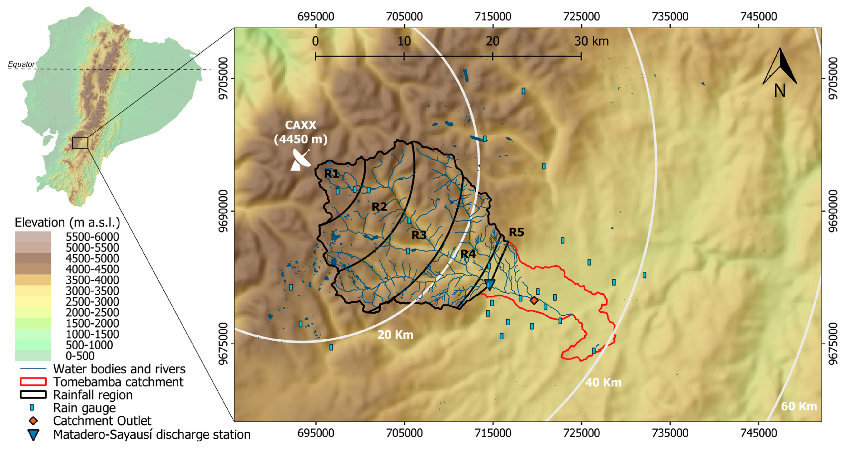
2.1. Study Site

The study was conducted in the Tomebamba catchment, located at the southern Andes of Ecuador. The catchment has an approximate extension of 300 km² at the Matadero-Sayausí hydrological station as seen in Figure 1 and it is representative of medium scale mountain catchments. The elevation ranges from 2800 to 4100 m a.s.l. The city of Cuenca lies at its outlet and, thus, it is exposed to a high risk of floods. Mountain catchments in the tropical Andes provide vital watershed services to downstream communities [39]. In this case, the most important are potable and irrigation water supply. Additional details of the catchment climatology can be found in [29]. Figure 1 illustrates the study site and the instruments used in the current investigation.

2.2. Instruments and Data

2.2.1. Radar

Data from a rainfall radar located at 4450 m.a.s.l. on the Paragüillas peak in the north border of the Cajas National Park in southern Ecuador was used in the current study. The radar has a maximum range of 100 km and provides 1D polar images of raw reflectivity records as described in [35]. The bin resolution is 2 degrees’ azimuth and 100 m range, therefore a matrix of 180 × 1000 values is obtained every 5-min. Data are available from the period April 2015 to June 2017.

Radar data was used with the purpose of obtaining two different spatio-temporal series: one of radar reflectivity and another of radar rainfall retrievals, both at hourly scale. These data were used to derive the inputs of the models. The time series of reflectivity records was obtained from the application of a quality control procedure. For this, specific corrections related to both the clutter and attenuation effects over the native reflectivity records were performed. The reflectivity correction was achieved through the methodology used by Orellana-Alvear et al. [35] that deals with static and dynamic clutter. This allowed to remove unrealistic reflectivity measurements (e.g., spikes and at certain point attenuation issues) from the radar images. Henceforth for simplicity we will refer to the resulting time series as native radar data.

The series of radar rainfall depth was obtained by using the step-wise correction model used in Orellana-Alvear et al. [35] that applies clutter and attenuation correction. In addition, a bias adjustment was applied by using the rain gauge data defined below in Section 2.2.2. For this, the multiplicative bias correction model described in [40] was used. Finally, data was transformed from rainfall rate to rainfall depth. This entire process resembles the usual efforts of getting the best quantitative estimations of rainfall maps to be used in distributed models. Finally, an accumulation to hourly scale was performed for both spatio-temporal series, reflectivity, and rainfall depth from the 5-min resolution records.

2.2.2. Rain Gauges

A rain gauge network, comprised by 28 rain gauges of 0.1 mm resolution each, was used in this study. The rain gauges are unevenly distributed over the study site and its surroundings as illustrated in Figure 1. A time series of hourly rainfall was obtained for every rain gauge. Data from the period April 2015 to June 2017 were used to adjust the radar rainfall retrievals. Data were quality checked and operational monitoring was frequently performed during the study period.

2.2.3. Discharge

Discharge is measured in the Tomebamba river at the Matadero-Sayausí station located at 2693 m.a.s.l. (see Figure 1). Mean hourly discharge, calculated for the period 1997–2017, is 7 m³ s⁻¹ at this hydrological station which was permanently monitored to ensure data quality. Data from the period April 2015 to June 2017 at hourly time step was used as target variable for the models. All extreme discharge values found in the historical data were kept for the analysis. Available data was divided in training and testing periods for the modeling process. Thus, data used in the training phase corresponded to April 2015 to June 2016, while the last year—from July 2016 to June 2017—was used for the test phase. The latter constitutes an independent dataset that was not used for training the model. Consequently, it ensures the model’s performance evaluation on unseen data.

2.3. Methods

2.3.1. Random Forest Model for Discharge Forecasting

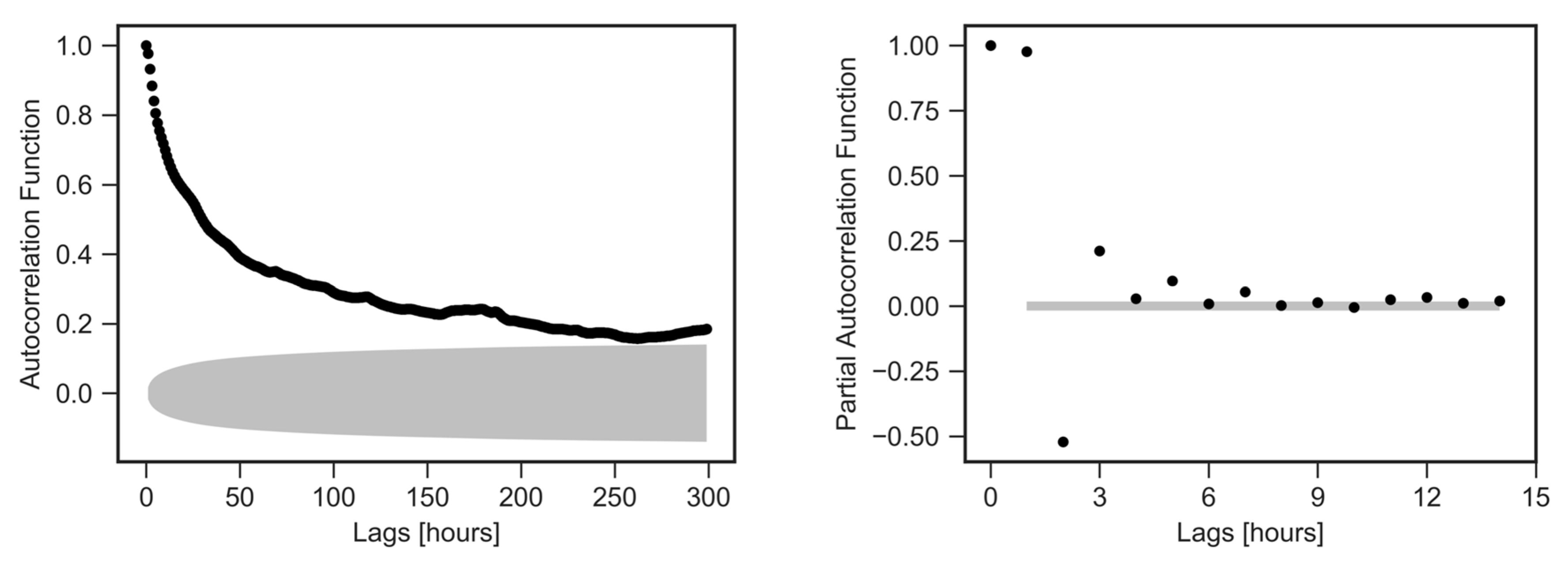
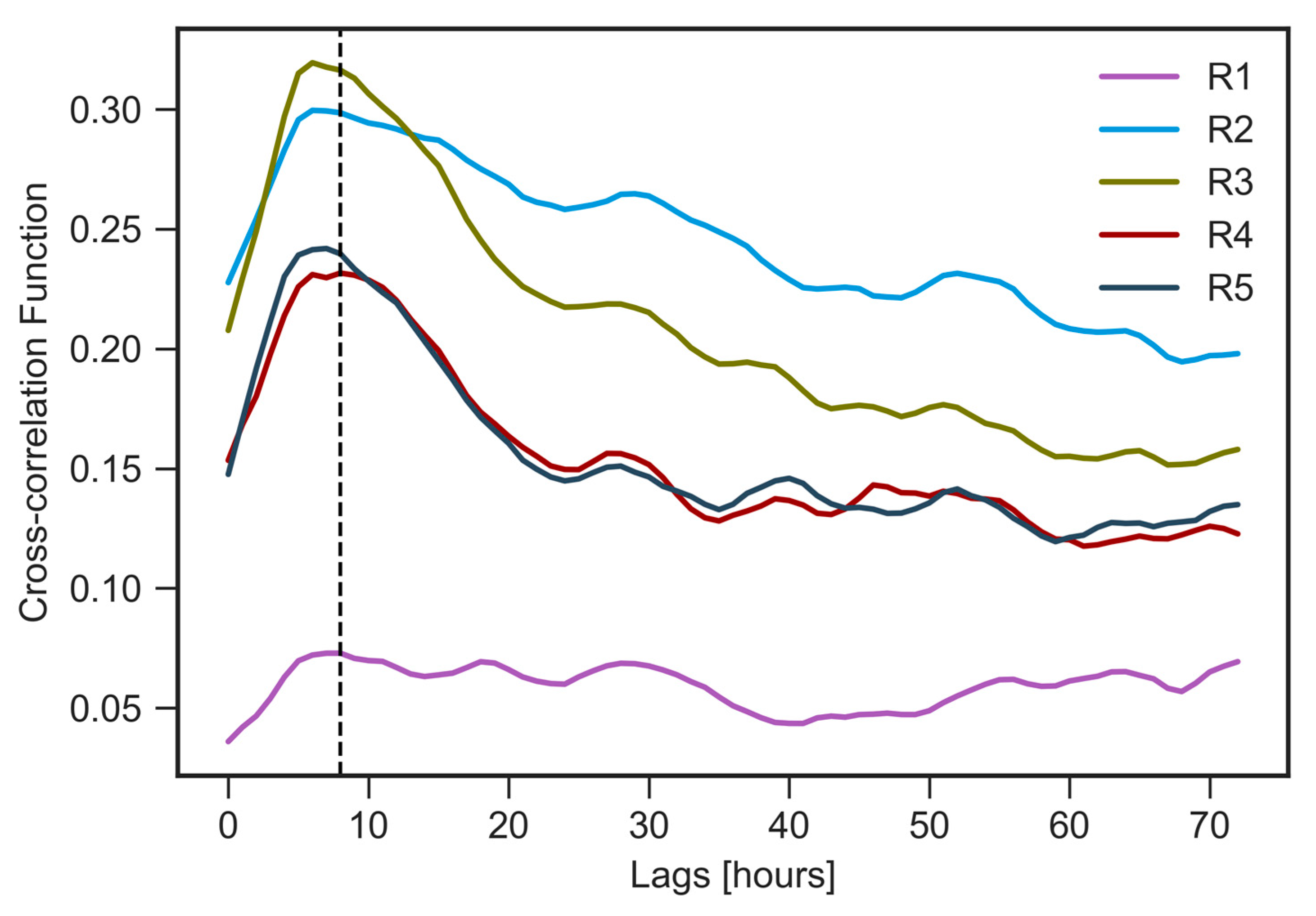
Random Forest (RF) is a decision tree-based model from the machine learning family. It is an ensemble method, which means that several trees (a forest) are built and the predicted estimation is the combination of the results of all tree models in the forest. The RF algorithm for regression derives n datasets of random samples with replacement (bootstrapping) from the original dataset. Then, these new datasets are used to build n trees, which ensures that a different subset is used for the construction of each decision tree of the model. A fraction of the data (out-of-bag, OOB), usually the 33%, is used for an internal validation process, which acts as independent data from the training process allowing obtaining unbiased estimations of the regression error. For building each regression tree, a random subset of N predictors (features) is used to create the binary rule at each node of the tree. The selection of the feature used for the binary rule at each step is based on the sum of square residuals. The tree is expanded until a certain depth has been reached (depth of the tree). Then, observations of the OOB subset are evaluated in each constructed tree; and the average of all estimations from the trees is the final estimation of the specific RF model. Finally, the performance of the RF model at the training stage is evaluated with a OOB score (i.e., metric of goodness of fit, here the coefficient of correlation R²) by comparing the estimations of the RF model and the corresponding observations of the OOB dataset. Therefore, n trees (i.e., number of trees), N features (i.e, number of random predictors used at each node to construct each tree) and the depth of the tree (i.e., limit of nodes in each tree) act as hyper-parameters that need to be optimized on the model, which is accomplished by a grid search approach that uses the OOB score for ranking all possible RF models.

For a more detailed explanation of how RF works the reader is referred to [41] in general, and to Orellana-Alvear et al. [35] for an application to this study region in a related work. The RF algorithm was used to develop discharge forecasting models with a lead time of four hours. A flowchart of the models’ implementation is provided in Figure 2. The following sections provide details about input data and configurations of these models.

2.3.2. Input Data

To reduce the complexity of the spatial representation of the radar data, we decided to delineate several regions where each one can be considered to be a virtual rain gauge. Then, every time series is derived from the spatial mean of the region at each hourly time step. The definition of the regions is given by considering two factors: (i) The spatial distribution of the virtual rain gauges should resemble the most common distribution of rain gauges within mountain catchments (i.e., along the altitudinal gradient) and (ii) we assume that each virtual rain gauge corresponds to a rainfall region which could be influenced due to the altitude. Thus, we divided the Tomebamba catchment in five regions from the headwater to the outlet by drawing concentric circles of increasing radius of 5565 m. We cropped the last region (R5) up to the Matadero Sayausí discharge station. This small area coincides with the urbanized area of the catchment (see Figure 1). By using this regionalization, rainfall regions from R1-R5 have mean elevations of 4027, 3867, 3736, 3463, and 3033 m respectively.

The simplification of the radar image into rainfall regions is required for reducing the number of inputs to the model; the use of all radar pixels as individual inputs would produce high dimensionality issues that will increase the computational costs. We are aware that this regionalization scheme may be improved; however, this is out of the scope of this study whose main objective is to evaluate the potential of leveraging native reflectivity records from meteorological radars on data-driven discharge forecasting modeling.

Inputs for the model are commonly determined by analyzing the target variable (i.e., discharge) and its relation with lagged values from related time series (e.g., discharge and precipitation) [42]. This process allows retaining the most relevant observations in the model. For this, different analyses of correlation were carried out between the target variable and the derived-rainfall radar time series.

First, an autocorrelation and partial correlation analyses, as in Muñoz et al. [29], were applied from the autocorrelation function (ACF) and the partial autocorrelation function (PACF) for identifying the number of previous discharge observations that mostly influenced the discharge at the time of interest. Derivation of ACF and PACF has been already documented in studies related to data-driven models for discharge forecasting [43]. Both analyses serve as complementary tools to define the number of lags (hours) to be included in the model. The ACF allows identifying autoregressive patterns in the time series, while the PACF is aimed at identifying the extent of the lag influence. Second, a cross-correlation analysis between the discharge and, either the reflectivity or rainfall depth, allowed finding the number of influential lags from the virtual rain gauge time series. Finally, the use of an additional input that represents the soil moisture condition into a data-driven hydrological model has been previously documented [44,45,46] and proven to be efficient. Thus, in order to account for the soil moisture condition of the catchment, a 3-day precipitation accumulation was considered to be proxy. Therefore, a 3-day proxy per region was calculated through the virtual rain gauge time series. It means that the 3-day precipitation accumulation is derived by either the sum of radar reflectivity values or the radar rainfall estimates depending on the data type of the time series. We selected a 3-day window due to rainfall data availability. Since this accumulation is calculated from the observed radar imagery which has not been filled in any way (e.g., interpolation of missing radar images as a result of technical maintenance), we need a continuous time frame for such derivation that allows obtaining an acceptable number of instances for training the model.

Finally, it is worth mentioning that usually several years of rainfall-runoff records are needed for streamflow forecasting modeling when using physical-based models. However, in this study we are able to exploit the limited data of a very short time (2.5 years) because there are not aquifers in our study catchment which means discharge is mainly controlled by rainfall. This allowed us to obtain a good number of events for data-driven discharge forecasting for most of the flow duration curve.

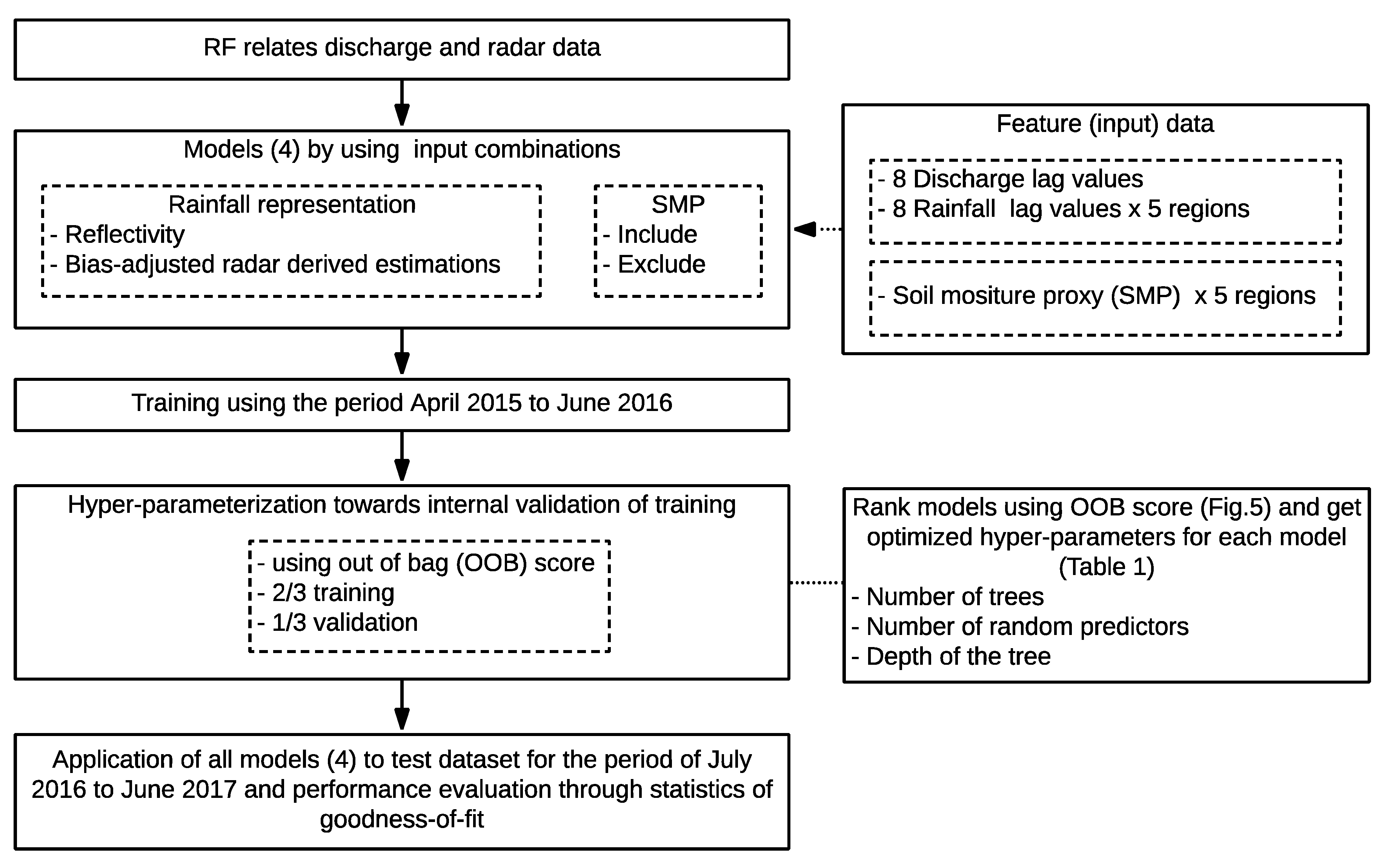
2.3.3. Input Data Configuration and Model Optimization

Four models were defined based on different input data scenarios. Input data configuration differs in two conditions: (i) data type of the time series (e.g., reflectivity (dBZ) or derived-rainfall radar (mm)) and (ii) inclusion or exclusion of the 3-day proxy variable. Therefore, four possible models were evaluated in the current study through the combination of the conditions mentioned above.

It should be pointed out that the number of lags resulting from the runoff and virtual rain gauge time series remained equal for all input data configurations. Thus, only the data representation (dBZ or mm) and the addition or omission of the 3-day proxy modify the inputs to the models.

The hyper-parameters of each model (i.e., number of trees, number of features and tree depth) were optimized using a grid search approach during the model training process. Thus, an independent set of optimized hyper-parameters was found for each model configuration. This ensured that each model accomplished the best possible use of its own input data.

2.3.4. Performance Evaluation

An independent evaluation was performed after the models were trained and optimized. For this, a discharge prediction of each model was obtained at each time step (i.e., four hours) of the one-year data used for the test phase. Afterwards, the forecasted discharges were compared with the corresponding observations through several metrics of goodness of fit. Thus, Root Mean Squared Error (RMSE), Percentage Bias (PBIAS) and Mean Absolute Relative Error (MARE) were calculated. In addition, model performance statistics, which are commonly used in hydrological studies, were derived. These include the Nash-Sutcliffe efficiency (NSE), the Kling-Gupta efficiency (KGE) [47] and its modified version (KGE′) [48] as described in Equations (1)–(3).

$$\mathrm{NSE}=1-\frac{{{\displaystyle \sum }}_{i=1}^n{\left(Qsi{m}_i-Qob{s}_i\right)}^2}{{{\displaystyle \sum }}_{i=1}^n{\left(Qob{s}_i-\overline{Q}obs\right)}^2}$$

(1)

where n is the length of the evaluated time series, Qsim_i and Qobs_i is the simulated and observed discharge at time i respectively, and $\overline{Q}obs$ is the mean of the observed values.

$$\mathrm{KGE}=1-\sqrt{{\left(r-1\right)}^2+{\left(\beta -1\right)}^2+{\left(\alpha -1\right)}^2}$$

(2)

$$\mathrm{KGE}\prime =1-\sqrt{{\left(r-1\right)}^2+{\left(\beta -1\right)}^2+{\left(\gamma -1\right)}^2}$$

(3)

where r is the Pearson correlation coefficient, β is the ratio between the means of the simulated values and the observed ones, α is the ratio between the standard deviations of the simulations and observations. Similarly, in Equation (3) γ is the ratio between the coefficients of variation (CV) of the simulated values to the observed ones. Thus, the decomposition of the KGE equations into correlation (r), bias (β) and variability (α/γ) facilitates to identify the relative importance of each independent metric over the derived KGE value.

3. Results and Discussion

In the following, the analysis of the models’ construction as well as their optimization process is documented. Moreover, the discharge forecasting models are evaluated and compared at first in terms of the radar data type, reflectivity, or rainfall depth, used as input for each model and secondly, regarding the use of the soil moisture proxy (i.e., 3-day precipitation accumulation) as additional input into the models.

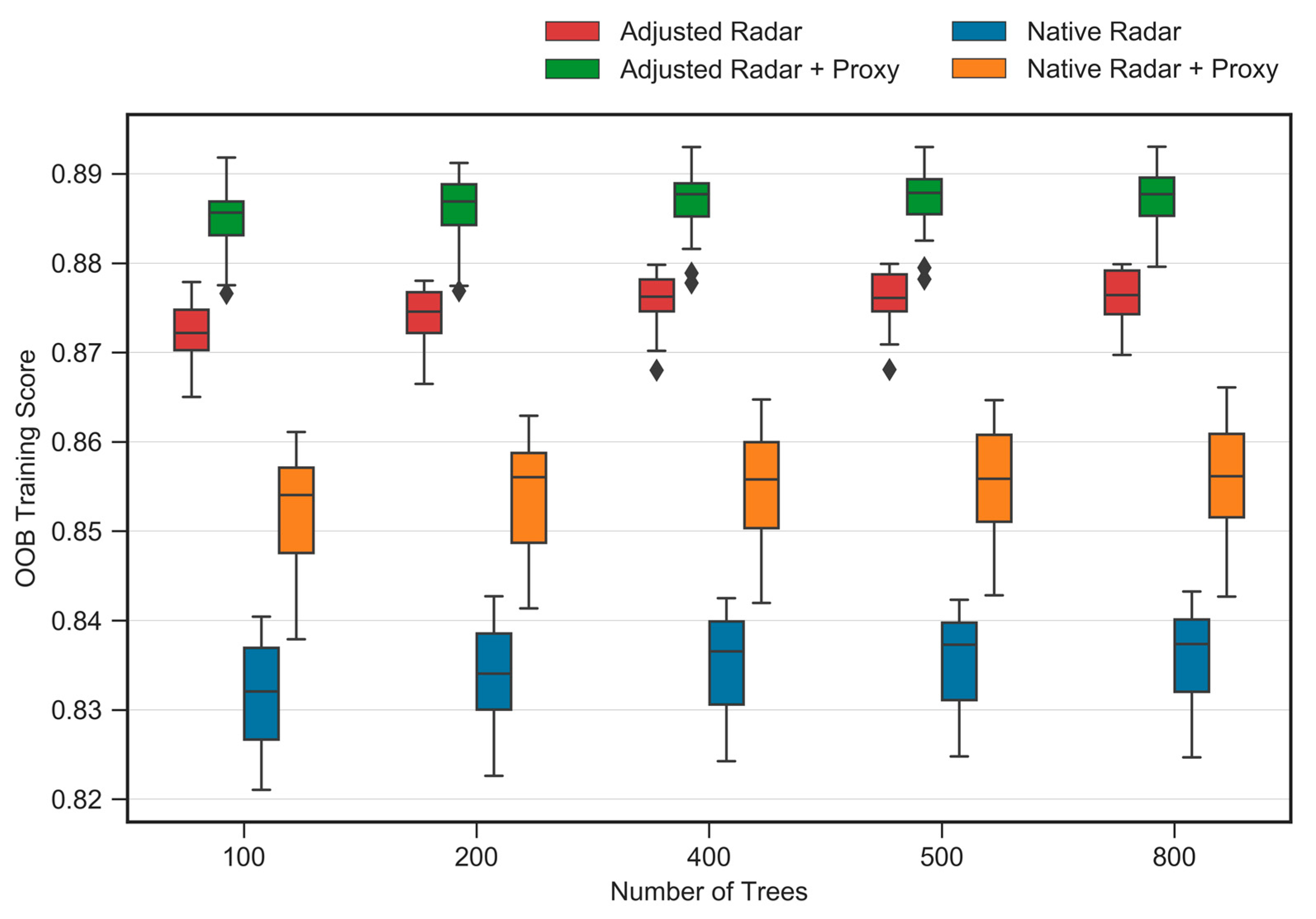
3.1. Feature Selection and Model Optimization

The number of precipitation and discharge lags for the inputs of the model were determined as eight lags (hours) for both discharge and precipitation variables. As seen in Figure 3, the 95% confidence interval (i.e., values out of the gray area are considered very probably a correlation and not a statistical chance) from the ACF in the left hand side reveals a correlation up to around 250 lags showing a dominant autoregressive pattern. In addition, the results of PACF illustrated in the right hand side of Figure 3 reveal no significant correlation from lag 8. These results are in agreement with Muñoz et al. [29] that used a slightly larger dataset of this discharge time series.

Furthermore, Figure 4 illustrates the Pearson cross-correlation analysis between the discharge time series and the one derived from the native radar data as a virtual rain gauge. Similar results were found when using the adjusted radar data. It can be seen that the highest correlation is found between lags 4 and 8 depending on the virtual rain gauge (i.e., rainfall region). Muñoz et al. [29] already discussed the relation of lag 4 to the mean concentration time of the catchment. However, in contrast to that study, we decided to keep eight lags from the precipitation variable because of the slight variability among rainfall regions. R1 has a lower correlation which could be related to three aspects: (i) the presence of a few tributaries in this region; (ii) its smaller area that drains to a location where there is an important presence of lakes that heavily affect water flow and transit times and; (iii) rainfall in the headwaters falls mainly as drizzle. Nonetheless, we maintained this layer because we aimed to build the models as simply and homogenously as possible, so that we can mainly focus on the input data type influence (i.e., native or adjusted radar data). In summary, the inputs for each model correspond to the values of the eight discharge lags (hours) and eight derived precipitation (or reflectivity) lags. The latter applies for every region (R1–R5). Thus, we defined [8 + (8 × 5)] inputs for modeling, which could increase in 5 due to the soil moisture proxy (i.e., one soil moisture proxy per region).

Figure 5 shows the convergence of the best hyper-parameters for all forecasting model configurations at 4 h in advance. The distribution of the OOB score for each number of trees follows from the results of the combination with different number of features and depths of the tree. It can be seen that both models using adjusted radar data have smaller variability than the models using native radar data. OOB score slightly improves when using adjusted radar data (~0.04). Optimized hyper-parameters corresponding to the number of trees, number of features and depth of the tree, as well as OOB scores for the training phase are shown in

Table 1. Optimized hyper-parameters for the discharge forecasting models and their OOB score at the training phase.

Model	n Trees	N Features	Depth of Tree	OOB Score
Adjusted	400	18	40	0.88
Adjusted + proxy	400	30	40	0.89
Native	400	18	30	0.83
Native + proxy	400	36	30	0.85

.

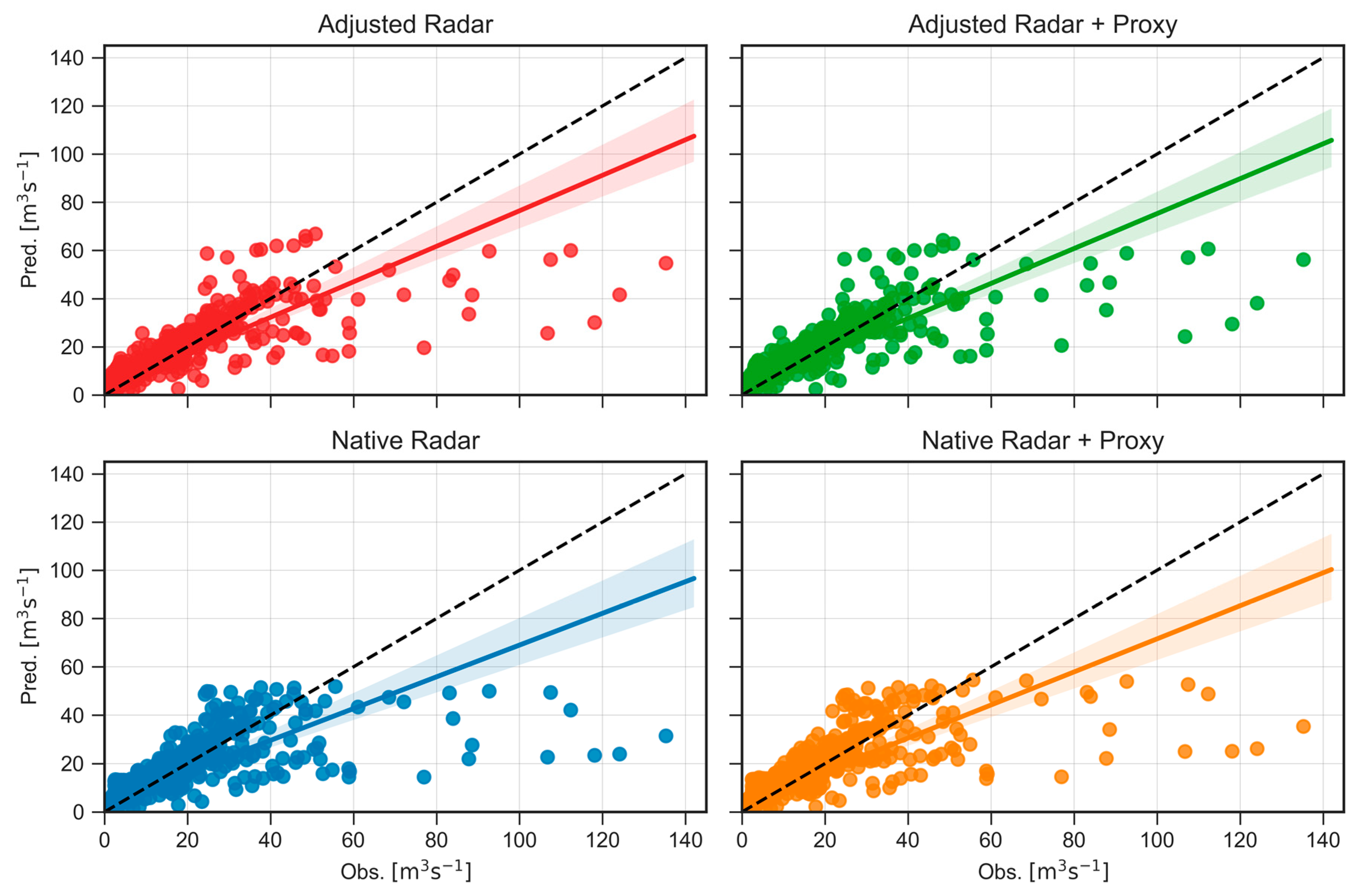
3.2. Performance Evaluation of Discharge Models with Test Data

In the following, the analyses are performed based on the evaluation of all four models by using the test dataset. The correlation between forecasted and observed values is illustrated in Figure 6 while the performance statistics of the models are summarized in

Table 2. Performance of all discharge forecasting models for the test period. * Metrics for the data subset where observations are higher than 50 m³ s⁻¹ are not shown due to the low number of samples.

Model	Data *	RMSE	PBIAS	MARE	NSE	Original KGE				Modif. KGE
						KGE	r	β	α	KGE′	γ
Adjusted	All	5.38	10.02	0.25	0.75	0.78	0.87	1.10	0.85	0.72	0.77
Adjusted + Proxy	All	5.33	9.87	0.25	0.75	0.77	0.87	1.10	0.83	0.71	0.76
Native	All	6.23	9.62	0.30	0.66	0.72	0.81	1.10	0.81	0.66	0.74
Native + Proxy	All	6.00	10.38	0.29	0.68	0.73	0.83	1.10	0.82	0.68	0.75
Adjusted	<50m3 s−1	3.08	16.26	0.22	0.84	0.81	0.94	1.16	1.08	0.81	0.93
Adjusted + Proxy	<50m3 s−1	3.04	17.27	0.24	0.85	0.81	0.94	1.17	1.04	0.79	0.89
Native	<50m3 s−1	3.47	17.06	0.26	0.8	0.80	0.92	1.17	1.05	0.79	0.90
Native + Proxy	<50m3 s−1	3.53	20.51	0.29	0.8	0.77	0.92	1.21	1.05	0.75	0.87

.

Figure 6 points out the slight differences between the models. The 95% confidence interval of the regression for the native radar data-based models is wider than their counterparts. Moreover, it can be observed that the scatter at all models starts to decouple at 25 m³ s⁻¹, with two branches, a lower and a higher. Finally, the lower retains all measurements higher than 50 m³ s⁻¹ which means that all models underestimate the discharge above this threshold. These observations of high discharge values will be discussed in detail later on.

Adjusted radar data-based models are in general slightly better than the native radar data-based models as shown in Table 2. Nonetheless, the component r from the KGE index reveals that differences in the models’ performance are mainly related to the linear correlation between forecasted and observed values. Thus, for the adjusted radar data-based models r reaches 0.87, while for native radar data-based models 0.81 < r < 0.83. The PBIAS oscillates around 10% for all models, while the MARE values increase up to 30% because of the absolute value of the error. Unexpectedly, the performance (NSE, KGE and KGE′) of the adjusted radar data-based model that uses the moisture proxy as additional input is equal or lower than the one that do not use the moisture proxy. In contrast, the native radar data-based model has, in general, a consistent improvement at all evaluation metrics when the proxy is included. This points out to the inherent error related to the rainfall adjustment process from the reflectivity values toward the bias correction based on the rain gauge data, which is present in the adjusted radar data-based models. It may be the case that while certain spatial points are properly adjusted regarding the rainfall quantities, this process also adds errors (i.e., inadequate bias correction) to other regions of the radar imagery. This in turns obscures the influence of the proxy within the adjusted radar data-based models. It is because the soil moisture proxy is indeed dependent of the adjusted rainfall and while the proxy may improve the discharge forecasting for some rainfall events, it may also have the contrary effect.

At first sight, the performance statistics of the models depicted in Table 2 seems slightly lower than other related studies in Andean regions such as Mejía-Veintimilla et al. [22] that accomplished a 0.77 < NSE < 0.80 for three different runoff events by using radar data. However, by exploring the discharge observations higher than 50 m³ s⁻¹ depicted in Figure 6, it turns out that they correspond only to 1% of the test dataset. From this sample, all observations higher than 60 m³ s⁻¹ (67% of the data) belong exclusively to two very strong rainfall events that occurred in 2017. When these very extreme events are omitted, the performance statistics improve substantially. For instance, for the Adjusted + Proxy model, NSE increases from 0.75 to 0.85, KGE increases from 0.77 to 0.82 and KGE′ improves from 0.71 to 0.80. Similarly, for the Native + Proxy model, the same metrics improved from 0.68 to 0.81, 0.73 to 0.80 and 0.68 to 0.79 respectively. Interestingly, for both models the γ component of KDE’ improves to ~0.90 which means that the CV between observations and predictions is comparable. Despite the fact that our results cannot be directly compared to those of Mejía-Veintimilla et al. [22] that used distributed models, it is worth mentioning that the random forest models in the current study have been evaluated toward the entire discharge time series and show satisfactory results (KDE~0.80, NSE > 0.80) for discharges lower than 50 m³ s⁻¹. This points out to the leverage of the radar data (even as native variable) and the usefulness of the simplified structure of the random forest models. Altogether, the differences in the performance of the random forest models are even smaller when considering discharge values lower than 50 m³ s⁻¹. Therefore, it confirms that the use of native radar data-based data as inputs for the models are able to produce as good results as those based on adjusted radar data.

Independently of the hydrological model, very high runoff events are always challenging to simulate [15,49]. In our study site, discharge of 50 m³ s⁻¹ is exceeded less than 5.4% of the time by considering a long-term series of more than 23 years at Matadero-Sayausí station. Nonetheless, in order to learn from these particular events and provide a potential explanation of the diminished performance of the models, we investigated from the radar imagery the event of 2017.04.13 that produced discharge values higher than 60 m³ s⁻¹ (see Figure 7). It is evident that a strong radar signal attenuation may compromise the reflectivity records for several hours of the event (i.e., heavy rainfall cores closer to the radar site). On the other hand, the rainfall adjustment based on rain gauge data at ground may not properly describe the spatial distribution and size of the strongest rain cells. Also, at certain time steps the rain cells are occurring very close to the outlet of the catchment, producing a flash discharge response, shorter than the 4 h lead time of our models, which heavily compromise their forecasting capability. In these cases, a precipitation nowcasting should be beneficial to the model in order to anticipate heavy rainfall events as in Heuvelink et al. [6]. In addition, the lower performance of all models for these extreme events is probably due to the small number of training samples of high discharge values (>50 m³ s⁻¹). As these events are infrequent, their particular characteristics regarding the velocity of the storm and spatial occurrence are not properly learned by the model. In addition, Guallpa et al. [31] showed that fast storms in the southern Andes of Ecuador need to be recorded by ground radar at higher temporal resolution (e.g., 1-min), otherwise the reliability of the reflectivity records and in consequence radar-derived rainfall was compromised. Moreover, as the RF discharge estimation is the result of the average of all predictions from the trees, it tends to underestimate high discharge values. Finally, it is worth mentioning that despite a less accurate forecast was accomplished for discharge peaks higher than 50 m³ s⁻¹, local emergency services can still be benefited from the discharge forecasting developed in this study. It is because a flooding alert can already be emitted once the forecast has exceeded a certain threshold without the need for a very accurate quantitative estimation.

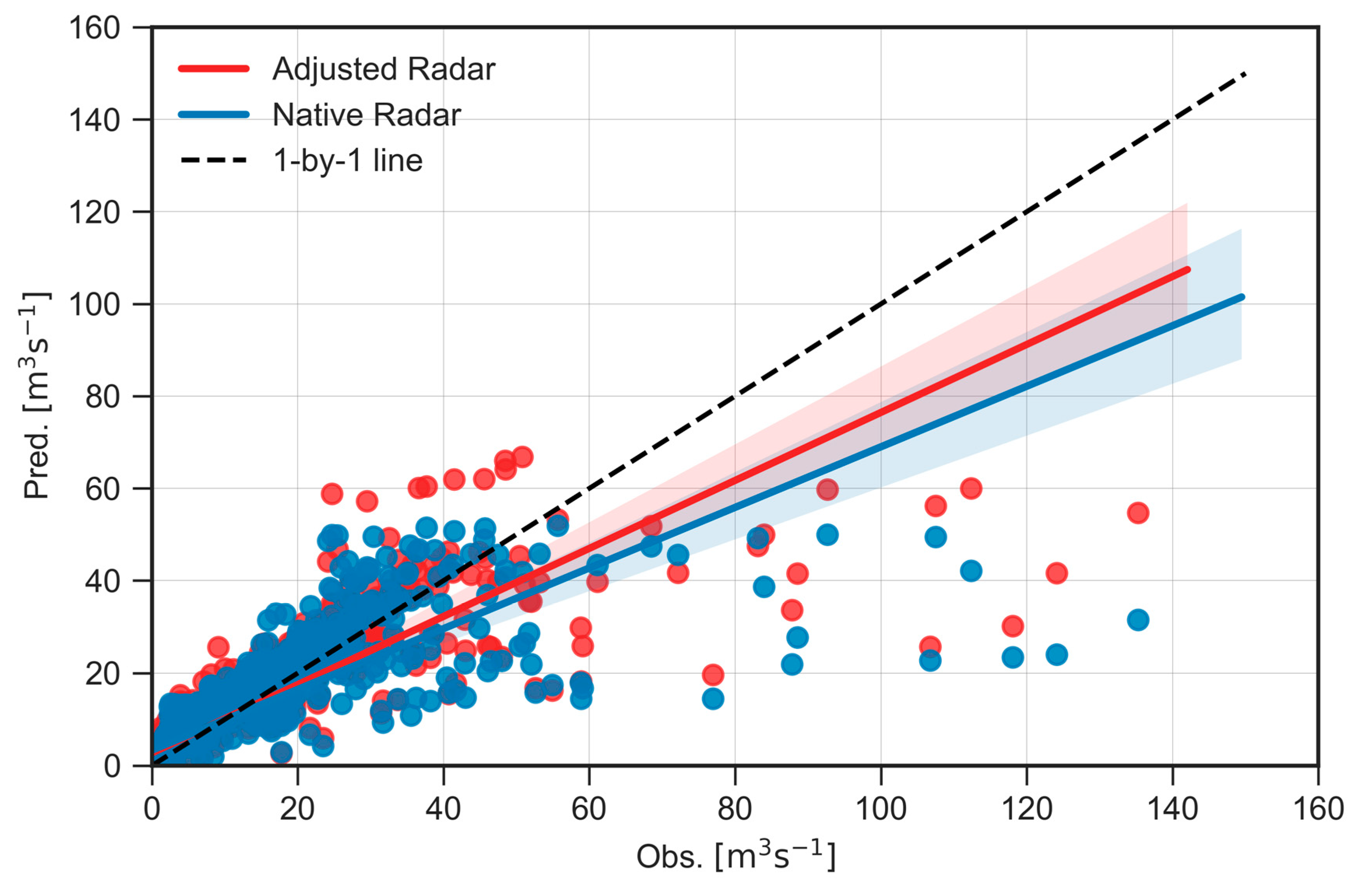
3.3. Data Type Influence

Figure 8 shows that the performance of the models that used native or adjusted radar data is very similar. Although the use of adjusted radar data slightly improves the runoff forecast, main differences occur in high discharges (>50 m³ s⁻¹). Below this threshold, the native radar data-based model denotes a lower scatter around the regression line whereas the adjusted radar data-based model tends to overestimate the discharge forecast. It could be a result of the added noise while applying the step-wise correction process to derive the adjusted rainfall radar data. On the other hand, better forecasts of higher discharge values may be benefited for the adjustment (bias removal) of rain rates by using the rain gauge records. For instance, by considering only the runoff observations higher than 50 m³ s⁻¹, the RMSE (PBIAS) from the Adjusted Radar + Proxy model are 44.46 (~−47%), while in contrast they are 49.95 (~−54%) for the Native Radar + Proxy model.

Altogether, the results bear out that the influence of data type might be overlooked (0.72 < KGE < 0.78; 0.66 < KGE′ < 0.72). This is an interesting finding since the pre-processing for the generation of input data for each model type (native- or adjusted radar) is quite different in terms of auxiliary data and correction process chain. The use of native radar data would be preferred due to the very few correction steps needed, which are mainly focused on fixing unrealistic observations. More importantly, the use of native data overcomes the problem of not having adequate rain gauge networks for radar image adjustment. This is of utmost importance because mountain remote areas, as the high Andes, are usually of very complex terrain and access.

3.4. Proxy of Soil Moisture Influence

A slight improvement in model performance by using the soil moisture proxy is observed in Figure 9. Nonetheless, this enhancement seems narrow due to the regionalization of the radar imagery. Other strategies by using soil moisture data derived from satellite such as in Jadidoleslam et al. [46] or derived from rainfall and evaporation as in Javelle et al. [44] are not feasible for this catchment due to its relatively small size and need for additional variables. Thus, different strategies of radar data regionalization are encouraged for future research since finding the optimal spatial representation is not the aim of the current study. Moreover, the limitation of the temporal length of the precipitation window (3-day precipitation accumulation) due to the number of samples could also influence the results. An adequate evaluation of an optimal window is also suggested for further studies.

4. Conclusions

A discharge forecast model by using a random forest algorithm by means of native radar data (i.e., reflectivity instead of derived rain rate) was developed and evaluated. In addition, a comparison with an equivalent model that used adjusted radar data (i.e., bias-adjusted radar derived rainfall) was performed. The use of an antecedent soil moisture proxy as input for the models was also evaluated. From the results, the following conclusions can be drawn:

(i) Similar goodness of fit was accomplished when using native radar data as well as adjusted radar data as input to the forecasting models. It demonstrates that the use of native radar data as input can properly map the expected discharge quantitatively. This is of great importance and interest since the need for exhaustive data pre-processing for converting the reflectivity values into rainfall depth can be omitted for discharge forecasting modeling applications using data-driven techniques.

(ii) Satisfactory results were obtained from the native radar data-based model (NSE = 0.81: KGE = 0.80) when evaluated in the discharge time series for values lower than 50 m³ s⁻¹. The decay in the model performance when considering higher discharge values was identified mainly as a result of two strong rainfall events. Several reasons could influence in the inadequate response of the model: (a) strong attenuation within the catchment, which lead to too low mean rainfall values for distant affected zones which coincides with the region close to the catchment outlet, (b) the reduced number or training samples for discharge values higher than 50 m³ s⁻¹ which complicates the RF model during its averaging of the predictions from the trees and (c) a suboptimal delineation of the rainfall regions for the virtual rain gauges’ derivation.

(iii) The inclusion of the derived soil moisture proxy used in this study (i.e., 3-day accumulation of precipitation) did not improve the model performance significantly, showing only a small increment in NSE at the expense of including an additional predictor. Given that the antecedent soil moisture condition affects the rainfall to runoff formation, more research is needed to address how to include an adequate soil moisture representation in the model configuration.

(iv) The RF model developed in this study is particularly suitable for its use in (remote) mountain regions where catchments usually remain scarcely monitored. Therefore, models that perform well in absence of (dense) rain gauge networks overcome a strong limitation in the application of simulation tools for disaster prevention through early warning systems. This can be extrapolated to other sites around the globe where limitations in access restrict the possibility of dense rain gauge monitoring.

In summary, this is a pioneer study that leverages the native radar variable (i.e., reflectivity) from a X-band single polarized radar located in the southern Andes of Ecuador for discharge forecasting by using a RF model. The usefulness of reflectivity records has been confirmed and highlights the benefits of leaving out the complexity of the radar rainfall process derivation. This means that the spatial-distributed rainfall pattern captured from ground radar can be used and applied without further pre-processing. It has enormous implications for remote and mountain regions in the world where additional monitoring can be expensive or even unaffordable and logistically challenging due to access issues. Moreover, the limitations of the RF model in situations with high attenuation (i.e., heavy rainfall events) were shown. This is comparable with the impact that the inadequate spatial distribution of precipitation—as a result of an uneven rain gauge network—has in physical-based models. This points out the relevance of the accuracy of the input data over the model itself. Thus, this study is a first step moving forward to focus the efforts on combining data sources (radar reflectivity and useful bias-adjusted radar rainfall areas) as inputs for discharge forecasting models. Further work will also focus on the improvement of the regionalization of precipitation and derivation of soil moisture through different techniques.

References

1. Paniconi, C.; Putti, M. Physically based modeling in catchment hydrology at 50: Survey and outlook. Water Resour. Res. 2015, 51, 2498–2514. [Google Scholar] [CrossRef] [Green Version]
2. Yaseen, Z.M.; El-shafie, A.; Jaafar, O.; Afan, H.A.; Sayl, K.N. Artificial intelligence based models for stream-flow forecasting: 2000-2015. J. Hydrol. 2015, 530, 829–844. [Google Scholar] [CrossRef]
3. Fatichi, S.; Vivoni, E.R.; Ogden, F.L.; Ivanov, V.Y.; Mirus, B.; Gochis, D.; Downer, C.W.; Camporese, M.; Davison, J.H.; Ebel, B.; et al. An overview of current applications, challenges, and future trends in distributed process-based models in hydrology. J. Hydrol. 2016, 537, 45–60. [Google Scholar] [CrossRef] [Green Version]
4. Valizadeh, N.; Mirzaei, M.; Allawi, M.F.; Afan, H.A.; Mohd, N.S.; Hussain, A.; El-shafie, A. Artificial intelligence and geo-statistical models for stream-flow forecasting in ungauged stations: State of the art. Nat. Hazards 2017. [Google Scholar] [CrossRef]
5. Mosavi, A.; Ozturk, P.; Chau, K.W. Flood prediction using machine learning models: Literature review. Water 2018, 10, 1536. [Google Scholar] [CrossRef] [Green Version]
6. Heuvelink, D.; Berenguer, M.; Brauer, C.C.; Uijlenhoet, R. Hydrological application of radar rainfall nowcasting in the Netherlands. Environ. Int. 2020, 136, 105431. [Google Scholar] [CrossRef]
7. Paz, I.; Tchiguirinskaia, I.; Schertzer, D. Rain gauge networks’ limitations and the implications to hydrological modelling highlighted with a X-band radar. J. Hydrol. 2020, 583, 124615. [Google Scholar] [CrossRef]
8. Sucozhañay, A.; Célleri, R. Impact of Rain Gauges distribution on the runoff simulation of a small mountain catchment in Southern Ecuador. Water 2018, 10, 1169. [Google Scholar] [CrossRef] [Green Version]
9. Li, Y.; Grimaldi, S.; Walker, J.P.; Pauwels, V.R. Application of remote sensing data to constrain operational rainfall-driven flood forecasting: A review. Remote Sens. 2016, 8, 456. [Google Scholar] [CrossRef] [Green Version]
10. Berne, A.; Krajewski, W.F. Advances in Water Resources Radar for hydrology: Unfulfilled promise or unrecognized potential? Adv. Water Resour. 2013, 51, 357–366. [Google Scholar] [CrossRef]
11. Editorial Board. Hydrologic applications of weather radar. J. Hydrol. 2015, 531, 231–233. [Google Scholar] [CrossRef]
12. Yoon, S.-S. Adaptive Blending Method of Radar-Based and Numerical Weather Prediction QPFs for Urban Flood Forecasting. Remote Sens. 2019, 11, 642. [Google Scholar] [CrossRef] [Green Version]
13. Khaki, M.; Hoteit, I.; Kuhn, M.; Forootan, E.; Awange, J. Assessing data assimilation frameworks for using multi-mission satellite products in a hydrological context. Sci. Total Environ. 2019, 647, 1031–1043. [Google Scholar] [CrossRef] [PubMed] [Green Version]
14. McKee, J.L.; Binns, A.D. A review of gauge–radar merging methods for quantitative precipitation estimation in hydrology. Can. Water Resour. J. 2016, 41, 186–203. [Google Scholar] [CrossRef]
15. Abon, C.C.; Kneis, D.; Crisologo, I.; Bronstert, A.; Primo, C.; David, C.; Heistermann, M.; Cristobal, C.; Kneis, D.; Crisologo, I.; et al. Evaluating the potential of radar-based rainfall estimates for streamflow and flood simulations in the Philippines. Geomat. Nat. Hazards Risk 2016, 7, 1390–1405. [Google Scholar] [CrossRef]
16. He, X.; Sonnenborg, T.O.; Refsgaard, J.C.; Vejen, F.; Jensen, K.H. Evaluation of the value of radar QPE data and rain gauge data for hydrological modeling. Water Resour. Res. 2013, 49, 5989–6005. [Google Scholar] [CrossRef]
17. Keblouti, M.; Ouerdachi, L.; Berhail, S. The use of weather radar for rainfall-runoff modeling, case of Seybouse watershed (Algeria ). Arab. J. Geosci. 2013. [Google Scholar] [CrossRef]
18. Hsu, S.Y.; Chen, T.B.; Du, W.C.; Wu, J.H.; Chen, S.C. Integrate Weather radar and monitoring devices for urban flooding surveillance. Sensors 2019, 19, 825. [Google Scholar] [CrossRef] [Green Version]
19. Chen, X.; Zhang, L.; Gippel, C.J.; Shan, L.; Chen, S.; Yang, W. Uncertainty of Flood Forecasting Based on Radar Rainfall Data Assimilation. Adv. Meteorol. 2016. [Google Scholar] [CrossRef] [Green Version]
20. Emmanuel, I.; Andrieu, H.; Leblois, E.; Janey, N.; Payrastre, O. Influence of rainfall spatial variability on rainfall-runoff modelling: Benefit of a simulation approach? J. Hydrol. 2015. [Google Scholar] [CrossRef]
21. Lobligeois, F.; Andréassian, V.; Perrin, C.; Tabary, P.; Loumagne, C. When does higher spatial resolution rainfall information improve streamflow simulation? An evaluation using 3620 flood events. Hydrol. Earth Syst. Sci. 2014, 18, 575–594. [Google Scholar] [CrossRef] [Green Version]
22. Mejía-Veintimilla, D.; Ochoa-Cueva, P.; Samaniego-Rojas, N.; Félix, R.; Arteaga, J.; Crespo, P.; Oñate-Valdivieso, F.; Fries, A. River discharge simulation in the high andes of southern ecuador using high-resolution radar observations and meteorological station data. Remote Sens. 2019, 11, 2804. [Google Scholar] [CrossRef] [Green Version]
23. Dinu, C.; Drobot, R.; Pricop, C.; Blidaru, T.V. Flash-Flood Modelling with Artificial Neural Networks using Radar Rainfall Estimates. Math. Model. Civ. Eng. 2017, 13, 10–20. [Google Scholar] [CrossRef] [Green Version]
24. Dinu, C.; Drobot, R.; Pricop, C.; Blidaru, T.V. Genetic Programming Technique applied for Flash-Flood Modelling using Radar Rainfall Estimates. Math. Model. Civ. Eng. 2017, 13, 27–38. [Google Scholar] [CrossRef] [Green Version]
25. Ragettli, S.; Zhou, J.; Wang, H.; Liu, C.; Guo, L. Modeling flash floods in ungauged mountain catchments
of China: A decision tree learning approach for parameter regionalization. J. Hydrol. 2017, 555, 330–346. [Google Scholar] [CrossRef]
26. Falck, A.S.; Maggioni, V.; Tomasella, J.; Diniz, F.L.; Mei, Y.; Beneti, C.A.; Herdies, D.L.; Neundorf, R.; Caram,
R.O.; Rodriguez, D.A. Improving the use of ground-based radar rainfall data for monitoring and predicting
floods in the Iguaçu river basin. J. Hydrol. 2018, 567, 626–636. [Google Scholar] [CrossRef]
27. Ogale, S.; Srivastava, S. Modelling and short term forecasting of flash floods in an urban environment. In Proceedings of the 2019 National Conference on Communications (NCC), Bangalore, India, 20–23 February 2019; pp. 1–6. [Google Scholar] [CrossRef]
28. Tyralis, H.; Papacharalampous, G.; Langousis, A. A brief review of random forests for water scientists and practitioners and their recent history in water resources. Water 2019, 11, 910. [Google Scholar] [CrossRef] [Green Version]
29. Muñoz, P.; Orellana-Alvear, J.; Willems, P.; Célleri, R. Flash-Flood Forecasting in an Andean Mountain
Catchment—Development of a Step-Wise Methodology Based on the Random Forest Algorithm. Water 2018, 10, 1519. [Google Scholar] [CrossRef] [Green Version]
30. Bendix, J.; Fries, A.; Zárate, J.; Trachte, K.; Rollenbeck, R.; Pucha-Cofrfrep, F.; Paladines, R.; Palacios, I.; Orellana, J.; Oñate-Valdivieso, F.; et al. RadarNet-Sur first weather radar network in tropical high mountains. Bull. Am. Meteorol. Soc. 2017, 98, 1235–1254. [Google Scholar] [CrossRef]
31. Guallpa, M.; Orellana-Alvear, J.; Bendix, J. Tropical andes radar precipitation estimates need high temporal and moderate spatial resolution. Water 2019, 11, 1038. [Google Scholar] [CrossRef] [Green Version]
32. Rollenbeck, R.; Bendix, J. Rainfall distribution in the Andes of southern Ecuador derived from blending weather radar data and meteorological field observations. Atmos. Res. 2011, 99, 277–289. [Google Scholar] [CrossRef]
33. Célleri, R.; Willems, P.; Buytaert, W.; Feyen, J. Space–time rainfall variability in the Paute basin, Ecuadorian Andes. Hydrol. Process. 2007, 21, 3316–3327. [Google Scholar] [CrossRef]
34. Orellana-Alvear, J.; Célleri, R.; Rollenbeck, R.; Bendix, J. Analysis of Rain Types and Their Z–R Relationships at Different Locations in the High Andes of Southern Ecuador. J. Appl. Meteorol. Climatol. 2017, 56, 3065–3080. [Google Scholar] [CrossRef]
35. Orellana-Alvear, J.; Célleri, R.; Rollenbeck, R.; Bendix, J. Optimization of X-Band Radar Rainfall Retrieval in the Southern Andes of Ecuador Using a Random Forest Model. Remote Sens. 2019, 11, 1632. [Google Scholar] [CrossRef] [Green Version]
36. Lo Conti, F.; Francipane, A.; Pumo, D.; Noto, L.V. Exploring single polarization X-band weather radar potentials for local meteorological and hydrological applications. J. Hydrol. 2015, 531, 508–522. [Google Scholar] [CrossRef]
37. Van de Beek, C.Z.; Leijnse, H.; Hazenberg, P.; Uijlenhoet, R. Close-range radar rainfall estimation and error analysis. Atmos. Meas. Tech. 2017, 9, 3837–3850. [Google Scholar] [CrossRef] [Green Version]
38. Chaipimonplin, T.; See, L.; Kneale, P. Improving neural network for flood forecasting using radar data on the Upper Ping River. In Proceedings of the 19th International Congress on Modelling and Simulation, Perth, Australia, 12–16 December 2011. [Google Scholar]
39. Hamel, P.; Riveros-Iregui, D.; Ballari, D.; Browning, T.; Célleri, R.; Chandler, D.; Chun, K.P.; Destouni, G.; Jacobs, S.; Jasechko, S.; et al. Watershed services in the humid tropics: Opportunities from recent advances in ecohydrology. Ecohydrology 2018, 11. [Google Scholar] [CrossRef]
40. Goudenhoofdt, E.; Delobbe, L. Evaluation of radar-gauge merging methods for quantitative precipitation estimates. Hydrol. Earth Syst. Sci. 2009, 13, 195–203. [Google Scholar] [CrossRef] [Green Version]
41. Breiman, L. Random forests. Mach. Learn. 2001, 45, 5–32. [Google Scholar] [CrossRef] [Green Version]
42. Tyralis, H.; Papacharalampous, G. Variable selection in time series forecasting using random forests. Algorithms 2017, 10, 114. [Google Scholar] [CrossRef] [Green Version]
43. Sudheer, K.P.; Gosain, A.K.; Ramasastri, K.S. A data-driven algorithm for constructing artificial neural network rainfall-runoff models. Hydrol. Process. 2002, 16, 1325–1330. [Google Scholar] [CrossRef]
44. Javelle, P.; Fouchier, C.; Arnaud, P.; Lavabre, J. Flash flood warning at ungauged locations using radar rainfall and antecedent soil moisture estimations. J. Hydrol. 2010, 394, 267–274. [Google Scholar] [CrossRef]
45. Ba, H.; Guo, S.; Wang, Y.; Hong, X.; Zhong, Y. Improving ANN model performance in runoff forecasting by adding soil moisture input and using data preprocessing techniques Huanhuan. Hydrol. Res. 2018, 49, 744–760. [Google Scholar] [CrossRef] [Green Version]
46. Jadidoleslam, N.; Mantilla, R.; Krajewski, W.F.; Goska, R. Investigating the role of antecedent SMAP satellite soil moisture, radar rainfall and MODIS vegetation on runo ff production in an agricultural region. J. Hydrol. 2019, 579, 124210. [Google Scholar] [CrossRef] [Green Version]
47. Gupta, H.V.; Kling, H.; Yilmaz, K.K.; Martinez, G.F. Decomposition of the mean squared error and NSE performance criteria: Implications for improving hydrological modelling. J. Hydrol. 2009, 377, 80–91. [Google Scholar] [CrossRef] [Green Version]
48. Kling, H.; Fuchs, M.; Paulin, M. Runoff conditions in the upper Danube basin under an ensemble of climate change scenarios. J. Hydrol. 2012, 424, 264–277. [Google Scholar] [CrossRef]
49. Ovando, A.; Tomasella, J.; Rodriguez, D.A.; Martinez, J.M.; Siqueira-Junior, J.L.; Pinto, G.L.; Passy, P.; Vauchel, P.; Noriega, L.; von Randow, C. Extreme flood events in the Bolivian Amazon wetlands. J. Hydrol. Reg. Stud. 2016, 5, 293–308. [Google Scholar] [CrossRef] [Green Version]
Figure 1. The Tomebamba catchment and delimitation of five rainfall regions at the Matadero-Sayausí discharge station.
Remotesensing 12 01986 g001
Figure 2. Workflow of the implementation of the RF models in the current study.
Remotesensing 12 01986 g002
Figure 3. Autocorrelation function (ACF) and Partial autocorrelation function (PACF) of the Matadero-Sayausí discharge series. Gray hatch indicates the 95% confidence band.
Remotesensing 12 01986 g003
Figure 4. Pearson cross-correlation comparison between the different precipitation time series (derived from the rainfall regions R1-R5 representing the virtual rain gauge stations) and the Matadero-Sayausí discharge station. The dashed line denotes lag 8.
Remotesensing 12 01986 g004
Figure 5. Evolution of the OOB score for different configuration models.
Remotesensing 12 01986 g005
Figure 6. Correlation between observed and forecasted discharge of the four different model configurations. The bisector line is showed in hatched black. The continuous lines denote the linear regressions and the shadow areas represent the 95% confidence interval band of each regression respectively.
Remotesensing 12 01986 g006
Figure 7. Hourly rainfall images from adjusted radar estimates corresponding to the rainfall event of 2017.04.13 (local time).
Remotesensing 12 01986 g007
Figure 8. Influence of the use of data type (adjusted or native—reflectivity—radar data) in the discharge forecasting models. The bisector line is showed in dotted black; the continuous lines denotes the linear regressions and the shadow areas represent the 95% confidence interval band of each regression respectively.
Remotesensing 12 01986 g008
Figure 9. Influence of the use of a soil moisture proxy variable in the discharge forecasting models. The bisector line is showed in dotted black; the continuous lines denotes the linear regressions and the shadow areas represent the 95% confidence interval band of each regression respectively.
Remotesensing 12 01986 g009