JL-GFDN: A Novel Gabor Filter-Based Deep Network Using Joint Spectral-Spatial Local Binary Pattern for Hyperspectral Image Classification

Abstract
:
1. Introduction
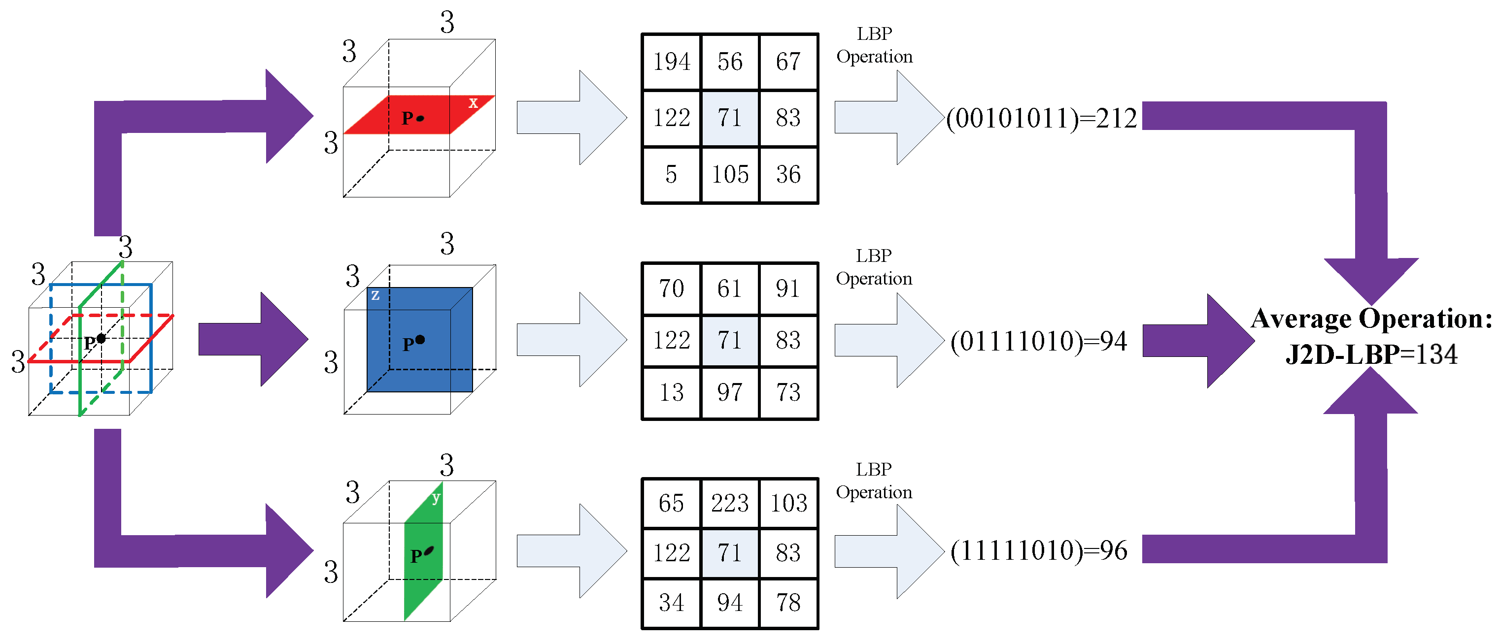
- To simultaneously depict the spectral and spatial characteristics of HSI, a joint spectral-spatial 2D-LBP feature, i.e., J2D-LBP is proposed based on averaging three 2D-LBP values associated with different planes.
- For further improving the performance of the original GFDN method, a novel HSI classification method JL-GFDN is built via using the framework of GFDN and J2D-LBP.
- Three different data sets are used to validate the effectiveness of JL-GFDN. Experimental results show that (i) the performance of J2D-LBP is superior to 2D-LBP and 3D-LBP; (ii) JL-GFDN holds a better classification performance than the traditional GFDN method.
2. Theoretical Background
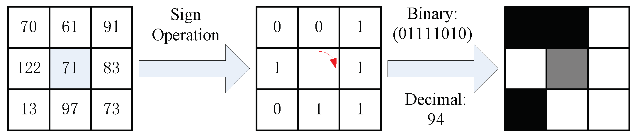
2.1. Two-Dimensional Local Binary Pattern (2D-LBP)
2.2. Gabor Filter-Based Deep Network (GFDN)
3. Methodology
3.1. Joint Two-Dimensional Local Binary Pattern (J2D-LBP)
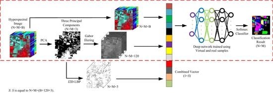
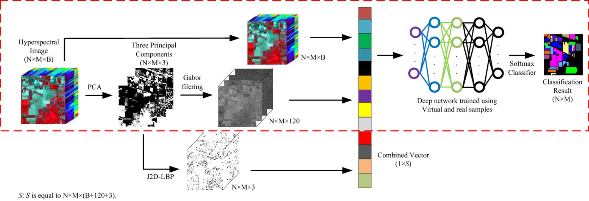
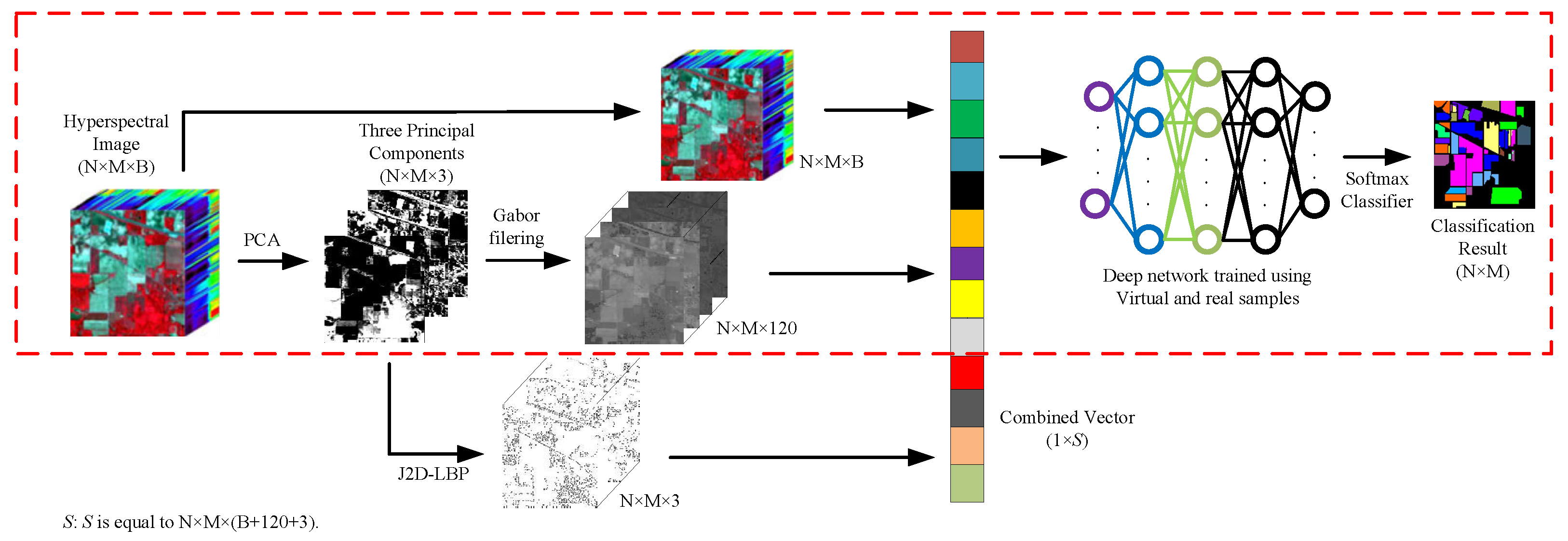
3.2. The Proposed Classification Method
- Input the HSI image (Size: N × M × B).
- Use PCA to reduce the dimensions of original HSI data and obtain the first three principal components (Size: N × M × 3).
- Extract GF features based on the first three principal components (Size: N × M × 120).
- Extract J2D-LBP features based on the first three principal components (Size: N × M × 3).
- Fuse the original HSI data, GF and J2D-LBP features together, and obtain one combined vector (Size: 1 × S, S = N × M × (B + 120 + 3)).
- Dependent on the combined vector, using the network to learn deep features and classify HSI.
- Output the classification result (Size: N × M).
4. Experiments
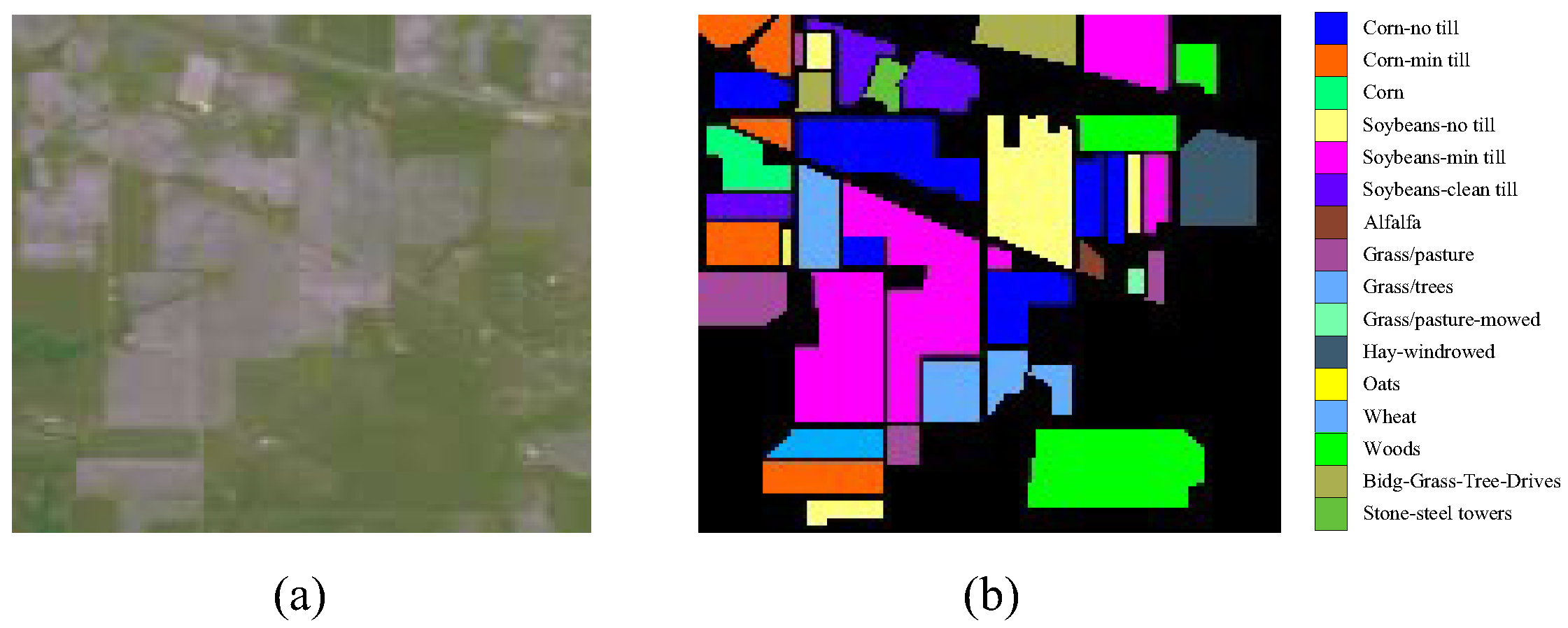
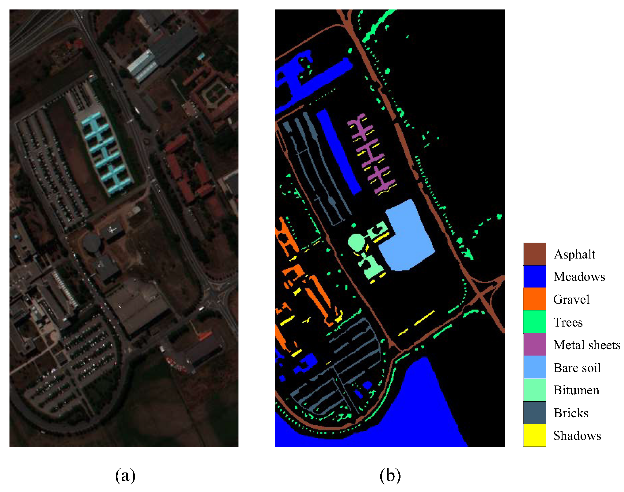
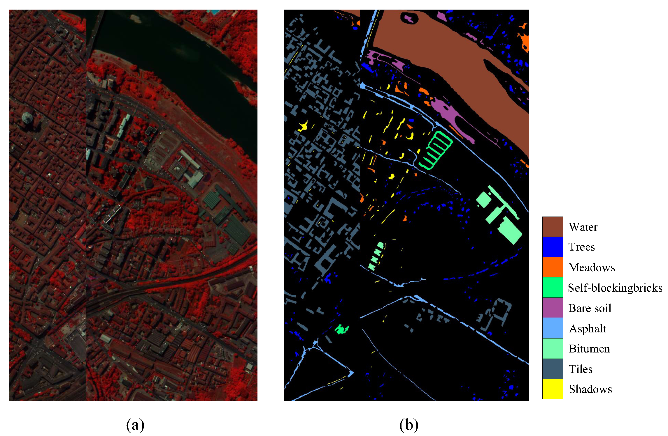
4.1. Data Sets
4.2. Experimental Analysis and Discussion
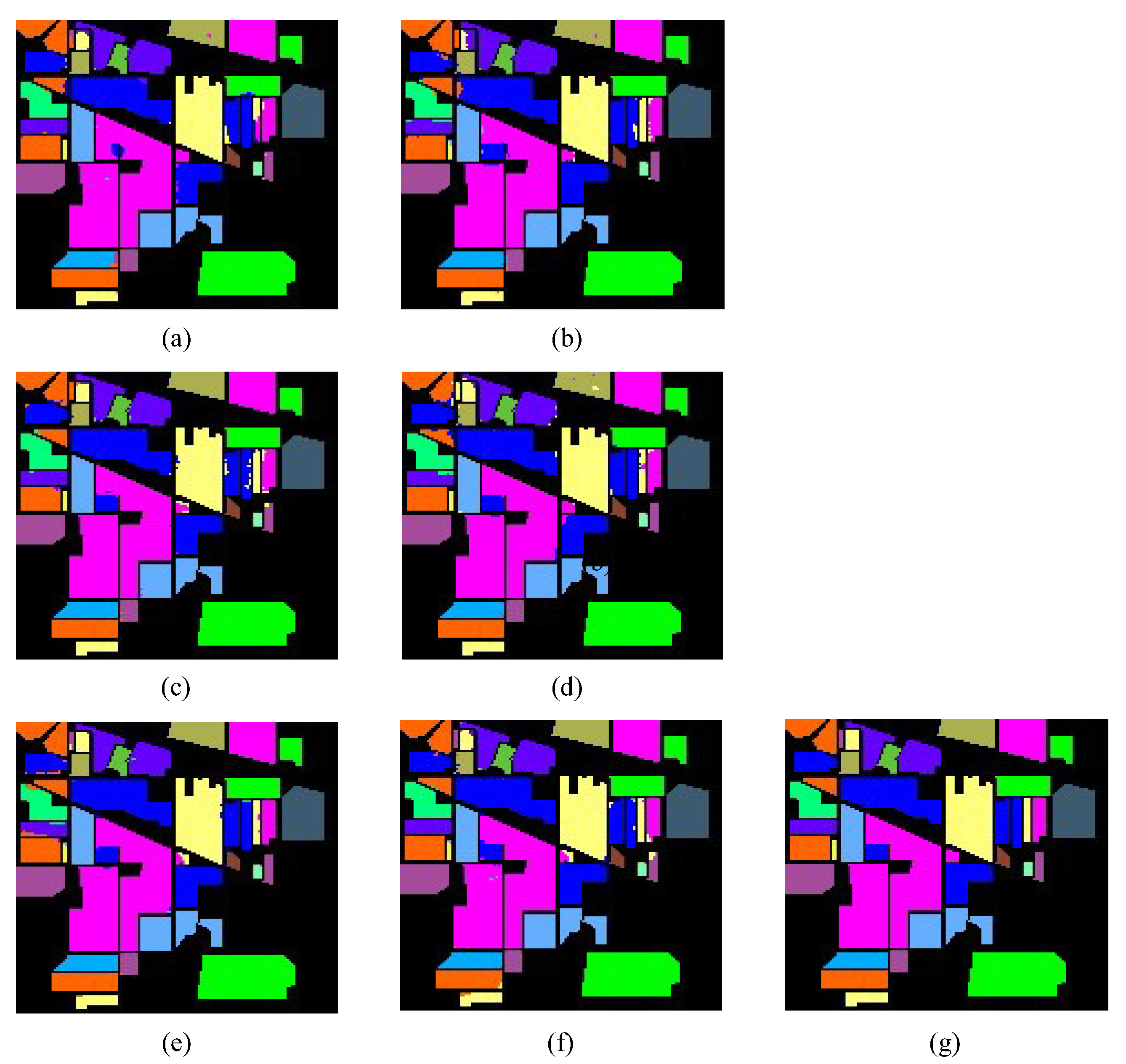
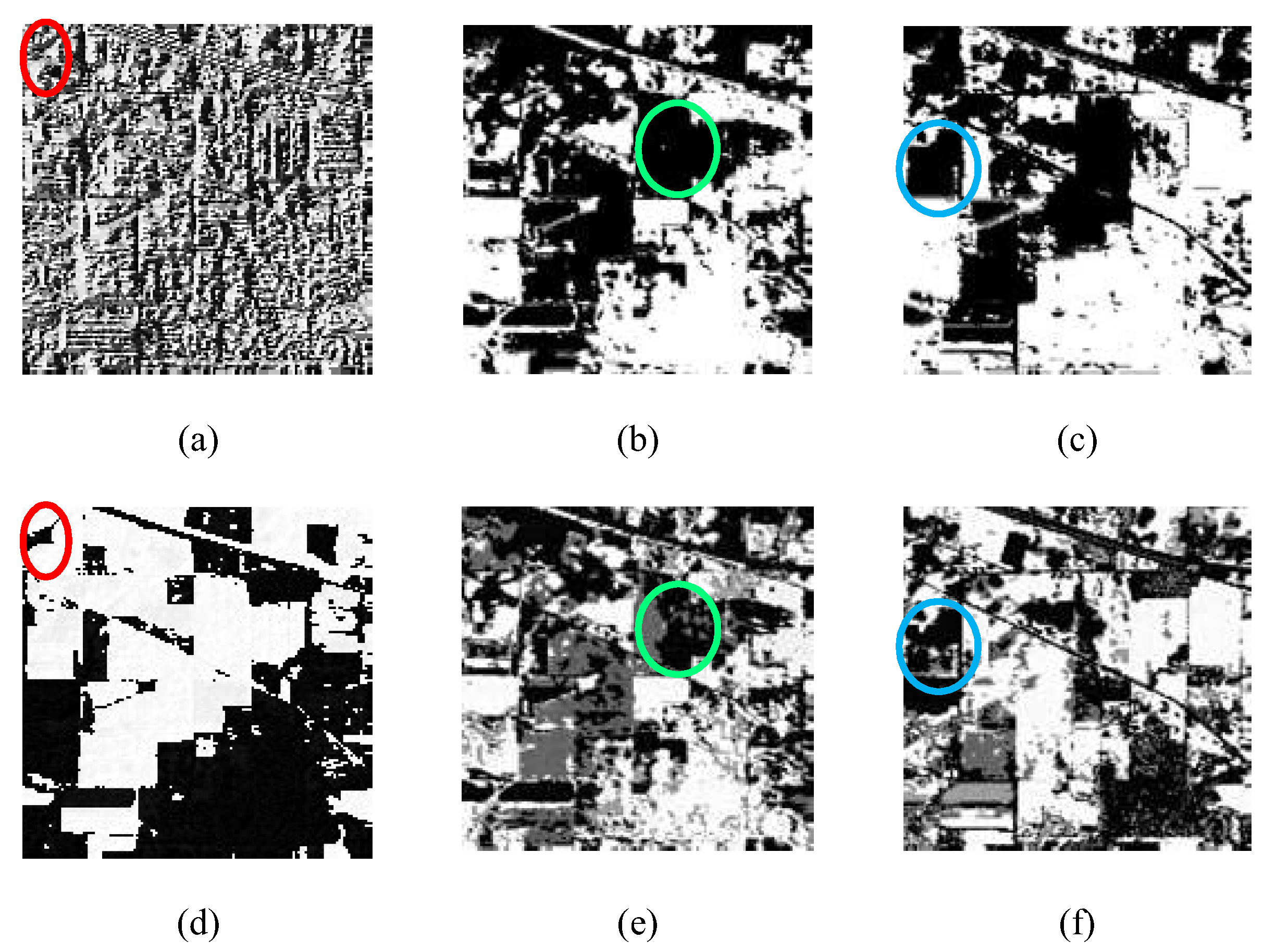
4.2.1. Experimental Results of Indian Pines
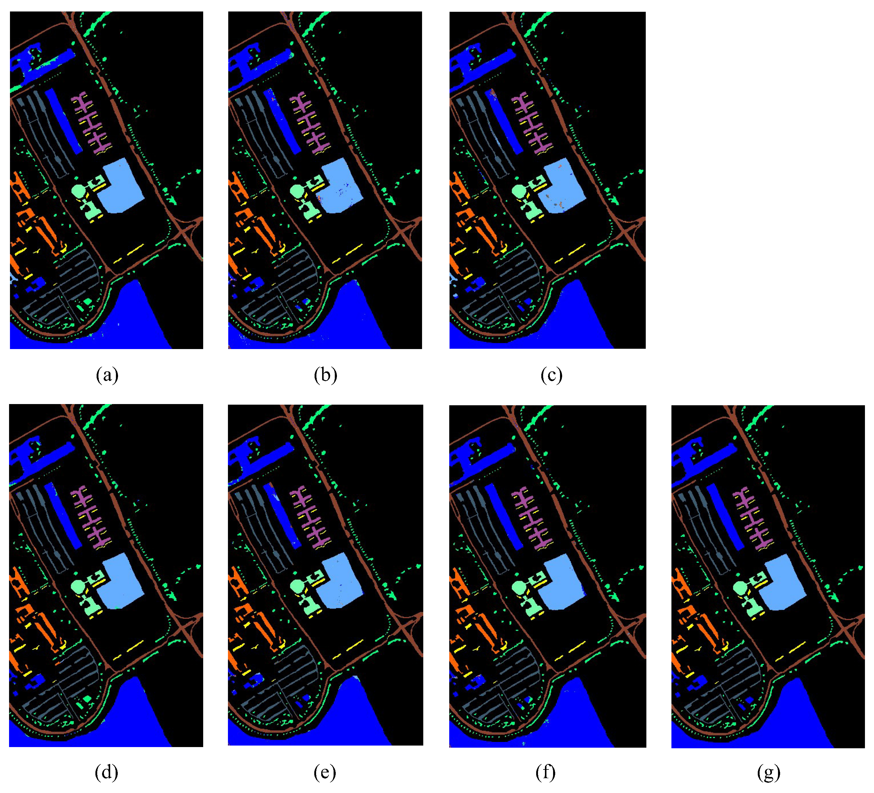
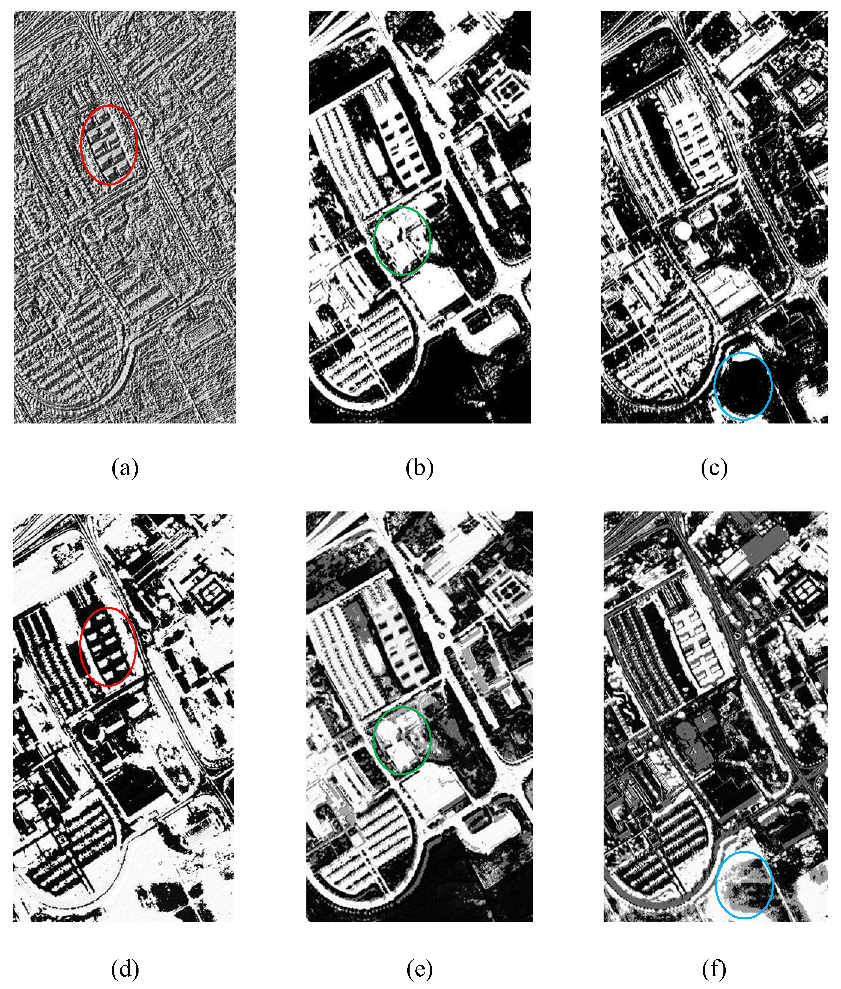
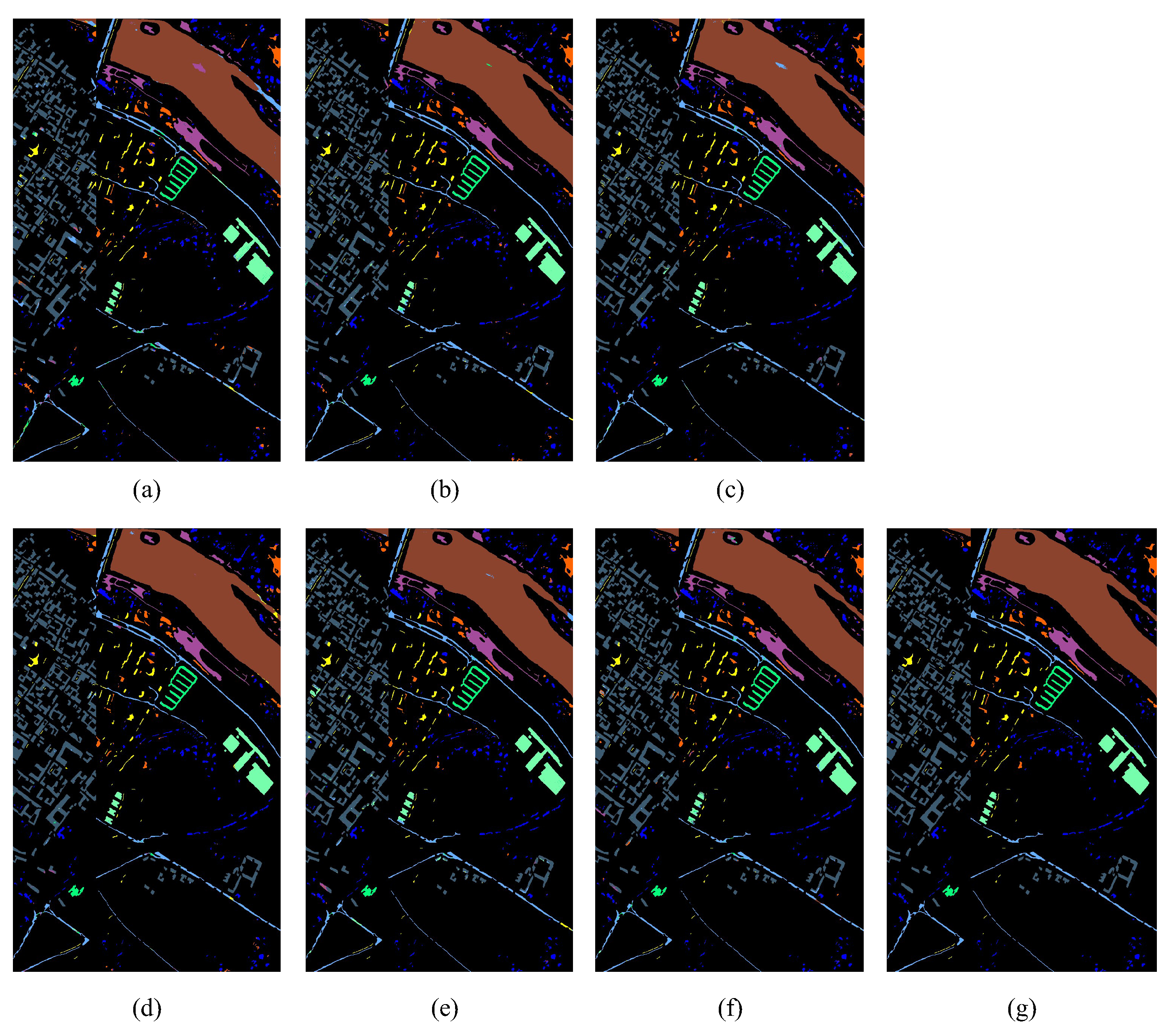
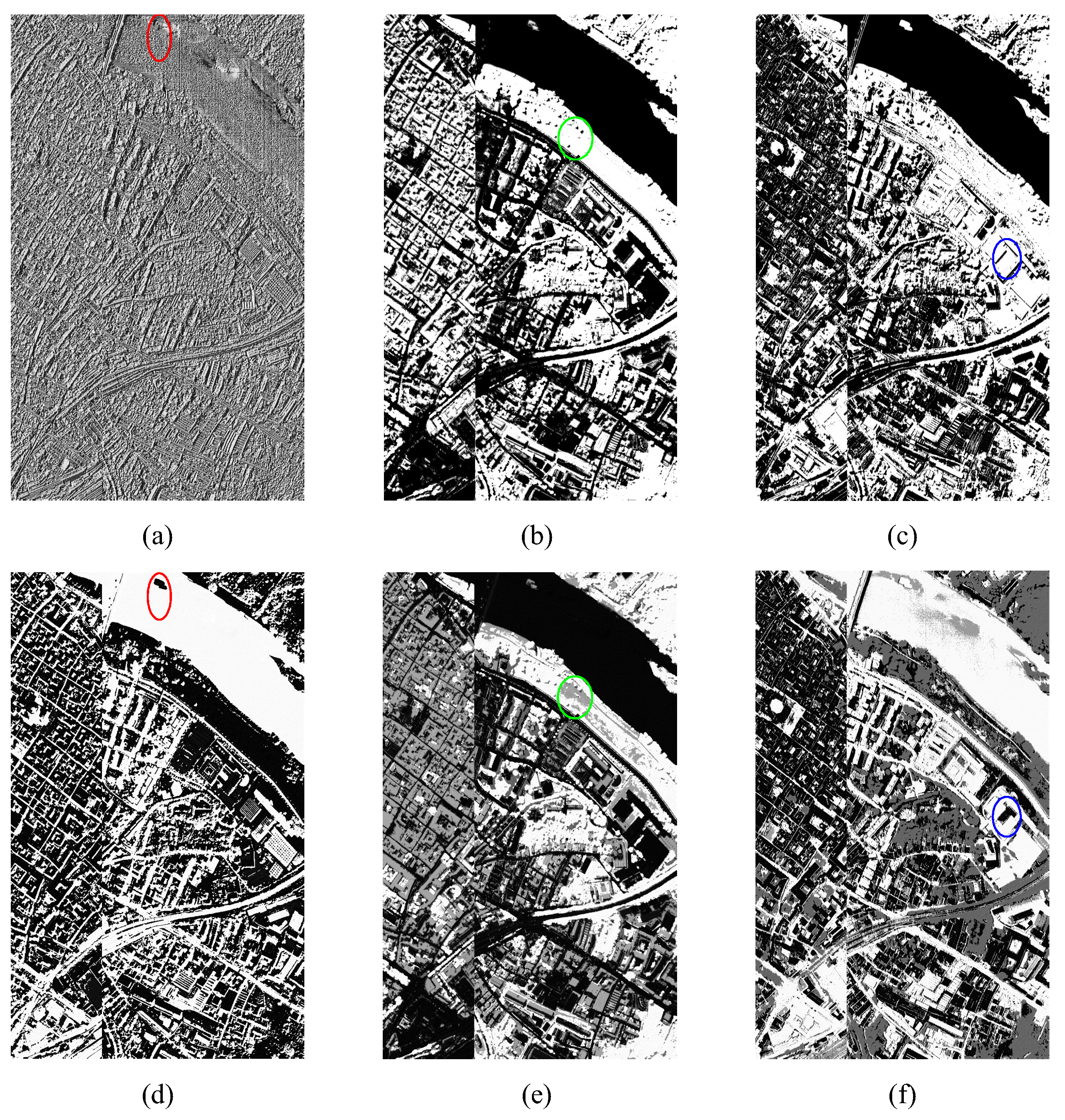
4.2.2. Experimental Results of the University of Pavia
4.2.3. Experimental Results of Pavia Center
5. Conclusions
Author Contributions
Funding
Acknowledgments
Conflicts of Interest
References
- Kaufman, J.R.; Eismann, M.T.; Celenk, M. Assessment of Spatial–Spectral Feature-Level Fusion for Hyperspectral Target Detection. IEEE J. Sel. Top. Appl. Earth Obs. Remote Sens. 2015, 8, 2534–2544. [Google Scholar] [CrossRef]
- Hughes, G. On the Mean Accuracy of Statistical Pattern Recognizers. IEEE Trans. Inf. Theory 1968, IT-14, 55–63. [Google Scholar] [CrossRef] [Green Version]
- Erchan, A.; Murat Can, O.; Berrin, Y. Deep Learning With Attribute Profiles for Hyperspectral Image Classification. IEEE Geosci. Remote Sens. Lett. 2016, 13, 1970–1974. [Google Scholar]
- Licciardi, G.; Marpu, P.R.; Chanussot, J.; Benediktsson, J.A. Linear Versus Nonlinear PCA for the Classification of Hyperspectral Data Based on the Extended Morphological Profiles. IEEE Geosci. Remote Sens. Lett. 2012, 9, 447–451. [Google Scholar] [CrossRef] [Green Version]
- Li, J.J.; Kingsdorf, B.; Du, Q. Band Selection for Hyperspectral Image Classification Using Extreme Learning Machine. Proc. SPIE 2017, 10198. [Google Scholar] [CrossRef]
- Du, Q.; Yang, H. Similarity-based Unsupervised Band Selection for Hyperspectral Image Analysis. IEEE Geosci. Remote Sens. Lett. 2008, 5, 564–568. [Google Scholar] [CrossRef]
- Jia, S.; Jie, H.; Zhu, J.S.; Jia, X.P.; Li, Q.Q. Three-dimensional Local Binary Patterns for Hyperspectral Imagery Classification. IEEE Trans. Geosci. Remote Sens. 2017, 55, 2399–2413. [Google Scholar] [CrossRef]
- Camps-Valls, G.; Gomez-Chova, L.; Munoz-Mari, J.; Vila-Frances, J.; Calpe-Maravilla, J. Composite Kernels for Hyperspectral Image Classification. IEEE Geosci. Remote Sens. Lett. 2006, 3, 93–97. [Google Scholar] [CrossRef]
- Kang, X.D.; Li, S.T.; Benediktsson, J.A. Spectral-Spatial Hyperspectral Image Classification with Edge-Preserving Filtering. IEEE Trans. Geosci. Remote Sens. 2014, 52, 2666–2677. [Google Scholar] [CrossRef]
- Fauvel, M.; Benediktsson, J.A.; Chanussot, J.; Sveinsson, J.R. Spectral and Spatial Classification of Hyperspectral Data Using SVMs and Morphological Profiles. IEEE Trans. Geosci. Remote Sens. 2008, 46, 3804–3814. [Google Scholar] [CrossRef] [Green Version]
- Mura, M.D.; Benediktsson, J.A.; Waske, B.; Bruzzone, L. Extended Profiles with Morphological Attribute Filters for the Analysis of Hyperspectral Data. Int. J. Remote Sens. 2010, 31, 5975–5991. [Google Scholar] [CrossRef]
- Liu, J.J.; Wu, Z.B.; Wei, Z.H.; Xiao, L.; Sun, L. Spatial-Spectral Kernel Sparse Representation for Hyperspectral Image Classification. IEEE J. Sel. Top. Appl. Earth Obs. Remote Sens. 2013, 6, 2462–2471. [Google Scholar] [CrossRef]
- Chen, Y.S.; Zhu, L.; Ghamisi, P.; Jia, X.P.; Li, G.Y.; Tang, L. Hyperspectral Images Classification with Gabor Filtering and Convolutional Neural Network. IEEE Geosci. Remote Sens. Lett. 2017, 14, 2355–2359. [Google Scholar] [CrossRef]
- Kang, X.X.; Li, C.C.; Li, S.T.; Lin, H. Classification of Hyperspectral Images by Gabor Filtering Based Deep Network. IEEE J. Sel. Top. Appl. Earth Obs. Remote Sens. 2018, 11, 1166–1178. [Google Scholar] [CrossRef]
- Li, W.; Chen, C.; Su, H.J.; Du, Q. Local Binary Patterns and Extreme Learning Machine for Hyperspectral Imagery Classification. IEEE Trans. Geosci. Remote Sens. 2015, 53, 3681–3693. [Google Scholar] [CrossRef]
- Ojala, T.; Pietikainen, M.; Maenpaa, T. Multiresolution Gray-scale and Rotation Invariant Texture Classification With Local Binary Patterns. IEEE Trans. Pattern Anal. Mach. Intell. 2002, 24, 971–987. [Google Scholar] [CrossRef]
- Grigorescu, S.E.; Petkov, N.; Kruizinga, P. Comparison of Texture Features Based on Gabor Filters. IEEE Trans. Image Process. 2002, 11, 116–1167. [Google Scholar] [CrossRef] [PubMed] [Green Version]
- Liu, C.; Wechsler, H. Gabor Feature Based Classification Using the Enhanced Fisher Linear Discriminant Model for Face Recognition. IEEE Trans. Image Process. 2002, 11, 467–476. [Google Scholar] [PubMed] [Green Version]
- Paoletti, M.E.; Haut, J.M.; Plaza, J.; Plaza, A. Deep Learning Classifiers for Hyperspectral Imaging: A Review. ISPRS J. Photogramm. Remote Sens. 2019, 158, 279–317. [Google Scholar] [CrossRef]


| Class | GFDN* | 2DLBP-GFDN* | 3DLBP-GFDN* | GFDN | JL-GFDN* | JL-GFDN |
|---|---|---|---|---|---|---|
| Alfalfa | 98.37 | 97.86 | 98.57 | 94.90 | 95.00 | 95.95 |
| Corn-N | 95.94 | 97.36 | 97.50 | 97.17 | 98.34 | 97.74 |
| Corn-M | 98.14 | 97.22 | 97.35 | 98.23 | 98.20 | 98.32 |
| Corn | 98.19 | 97.34 | 98.76 | 98.60 | 97.34 | 99.08 |
| Grass-P | 94.53 | 95.34 | 95.43 | 96.63 | 97.05 | 97.27 |
| Grass-T | 97.71 | 99.73 | 99.12 | 98.79 | 99.40 | 99.25 |
| Grass-P-M | 90.43 | 94.00 | 95.60 | 94.78 | 96.40 | 95.20 |
| Hay-W | 99.15 | 99.84 | 99.91 | 99.93 | 99.70 | 99.77 |
| Oats | 77.78 | 77.22 | 82.22 | 95.56 | 92.22 | 88.89 |
| Soybean-N | 95.27 | 97.16 | 96.98 | 96.70 | 97.14 | 96.98 |
| Soybean-M | 98.37 | 98.25 | 99.19 | 99.01 | 98.76 | 99.07 |
| Soybean-C | 95.99 | 95.76 | 97.69 | 97.32 | 96.67 | 97.80 |
| Wheat | 97.90 | 99.36 | 97.93 | 98.05 | 98.40 | 99.15 |
| Woods | 99.36 | 99.96 | 99.97 | 99.94 | 99.82 | 99.91 |
| Building-G-T-D | 97.11 | 97.64 | 98.17 | 98.57 | 98.14 | 98.65 |
| Stone-S-T | 88.16 | 93.65 | 98.71 | 95.63 | 97.88 | 98.82 |
| OA | 97.30 | 97.93 | 98.33 | 98.29 | 98.41 | 98.56 |
| AA | 95.15 | 96.11 | 97.07 | 97.49 | 97.53 | 97.62 |
| Kappa | 96.93 | 97.64 | 98.10 | 98.06 | 98.19 | 98.35 |
| Class | GFDN* | 2DLBP-GFDN* | 3DLBP-GFDN* | GFDN | JL-GFDN* | JL-GFDN |
|---|---|---|---|---|---|---|
| Asphalt | 98.35 | 98.74 | 97.81 | 98.47 | 98.18 | 98.80 |
| Meadows | 96.36 | 96.54 | 97.08 | 97.99 | 98.21 | 98.62 |
| Gravel | 98.97 | 99.26 | 99.59 | 99.87 | 99.60 | 99.55 |
| Trees | 97.07 | 97.77 | 97.47 | 98.38 | 97.88 | 98.52 |
| Metal sheets | 99.50 | 99.92 | 99.87 | 99.90 | 99.97 | 99.97 |
| Bare Soil | 99.26 | 99.18 | 98.84 | 99.13 | 99.09 | 98.85 |
| Bitumen | 99.76 | 99.86 | 99.95 | 99.96 | 99.58 | 99.69 |
| Bricks | 98.62 | 98.33 | 98.28 | 98.62 | 98.28 | 98.73 |
| Shadows | 97.74 | 99.91 | 99.91 | 99.93 | 99.89 | 99.80 |
| OA | 97.58 | 97.81 | 97.86 | 98.51 | 98.48 | 98.81 |
| AA | 98.40 | 98.83 | 98.76 | 99.14 | 98.97 | 99.17 |
| Kappa | 96.79 | 97.08 | 97.15 | 98.01 | 97.96 | 98.40 |
| Class | GFDN* | 2DLBP-GFDN* | 3DLBP-GFDN* | GFDN | JL-GFDN* | JL-GFDN |
|---|---|---|---|---|---|---|
| Water | 98.20 | 99.67 | 99.50 | 98.83 | 99.68 | 99.71 |
| Trees | 90.51 | 92.07 | 92.71 | 91.28 | 91.72 | 93.48 |
| Meadows | 94.43 | 95.41 | 93.86 | 94.47 | 95.61 | 95.57 |
| Bitumen | 97.15 | 98.17 | 97.13 | 97.89 | 98.36 | 98.70 |
| Bare soil | 97.88 | 99.14 | 98.79 | 98.00 | 98.88 | 98.97 |
| Asphalt | 91.32 | 94.58 | 92.75 | 92.08 | 95.24 | 94.85 |
| Self-blockingbrichs | 97.88 | 97.45 | 97.37 | 97.66 | 97.31 | 97.11 |
| Tiles | 96.27 | 96.84 | 98.01 | 96.54 | 97.44 | 97.63 |
| Shadows | 99.43 | 99.71 | 99.89 | 99.51 | 99.38 | 99.65 |
| OA | 96.72 | 97.90 | 98.02 | 97.18 | 98.09 | 98.22 |
| AA | 95.90 | 97.00 | 96.67 | 96.25 | 97.07 | 97.30 |
| Kappa | 95.41 | 97.04 | 97.21 | 96.04 | 97.30 | 97.49 |
© 2020 by the authors. Licensee MDPI, Basel, Switzerland. This article is an open access article distributed under the terms and conditions of the Creative Commons Attribution (CC BY) license (http://creativecommons.org/licenses/by/4.0/).
Share and Cite
Zhang, T.; Zhang, P.; Zhong, W.; Yang, Z.; Yang, F. JL-GFDN: A Novel Gabor Filter-Based Deep Network Using Joint Spectral-Spatial Local Binary Pattern for Hyperspectral Image Classification. Remote Sens. 2020, 12, 2016. https://0-doi-org.brum.beds.ac.uk/10.3390/rs12122016
Zhang T, Zhang P, Zhong W, Yang Z, Yang F. JL-GFDN: A Novel Gabor Filter-Based Deep Network Using Joint Spectral-Spatial Local Binary Pattern for Hyperspectral Image Classification. Remote Sensing. 2020; 12(12):2016. https://0-doi-org.brum.beds.ac.uk/10.3390/rs12122016
Chicago/Turabian StyleZhang, Tao, Puzhao Zhang, Weilin Zhong, Zhen Yang, and Fan Yang. 2020. "JL-GFDN: A Novel Gabor Filter-Based Deep Network Using Joint Spectral-Spatial Local Binary Pattern for Hyperspectral Image Classification" Remote Sensing 12, no. 12: 2016. https://0-doi-org.brum.beds.ac.uk/10.3390/rs12122016