PolSAR Image Classification Using a Superpixel-Based Composite Kernel and Elastic Net

Abstract

The presence of speckles and the absence of discriminative features make it difficult for the pixel-level polarimetric synthetic aperture radar (PolSAR) image classification to achieve more accurate and coherent interpretation results, especially in the case of limited available training samples. To this end, this paper presents a composite kernel-based elastic net classifier (CK-ENC) for better PolSAR image classification. First, based on superpixel segmentation of different scales, three types of features are extracted to consider more discriminative information, thereby effectively suppressing the interference of speckles and achieving better target contour preservation. Then, a composite kernel (CK) is constructed to map these features and effectively implement feature fusion under the kernel framework. The CK exploits the correlation and diversity between different features to improve the representation and discrimination capabilities of features. Finally, an ENC integrated with CK (CK-ENC) is proposed to achieve better PolSAR image classification performance with limited training samples. Experimental results on airborne and spaceborne PolSAR datasets demonstrate that the proposed CK-ENC can achieve better visual coherence and yield higher classification accuracies than other state-of-art methods, especially in the case of limited training samples.

1. Introduction

Since the polarimetric synthetic aperture radar (PolSAR) systems can transmit and receive electromagnetic signals in different polarization channels [1], the PolSAR datasets can provide more detailed information about the backscattering phenomena than data collected by single-channel SAR or other remote sensing systems [2]. The availability of PolSAR data stimulates intensive research in polarimetric analysis techniques and applications, including PolSAR target detection [3], change detection [4], polarization classification, and so on. In particular, the PolSAR image classification continues to be an active field of research [2].

In the remote sensing community, algorithms for PolSAR image classification are endless [5,6,7,8,9,10,11]. The feature extraction, as one important aspect of classification algorithms, has seen a lot of success and received sustained development [12]. The features used for PolSAR image classification include the polarization target decomposition (TD) features [5,13,14,15], the polarization data features [16,17], and so on [18,19]. Here, these feature extractions can be called explicit feature extractions [2], where features are extracted by projecting the PolSAR complex-valued data into the real domain. Broadly, in the explicit feature extraction aspect, the following problems may be encountered [2,20]. Firstly, the feature extraction process increases computation time and computational load. Secondly, features for special classification tasks that are hand-crafted and determined by plenty of experiments require manual trial and involve computational error. Finally, the feature extraction process cannot avoid the loss of valuable information [21].

Since the scattering characteristics of the distributed targets for PolSAR images can be described by their coherency or covariance matrix [22], it is reasonable to make classification algorithms work directly on these complex-valued (CV) matrices. At the same time, this can also ease the aforementioned problems caused by the explicit feature extraction from original PolSAR CV data. One choice is classification approaches based on statistical distribution assumption [7,21,23,24,25,26]. However, the common disadvantages of these methods are usually complicated parameter estimation and limited model applicability [27,28]. Recently, some classifiers with the training–testing format, which work directly on the PolSAR CV data, have constituted an active area of research [2,20,29,30,31,32,33,34]. Among them, complex-valued networks provide results comparable to networks designed for real-valued input [32,33,34]. Although these methods have achieved remarkable breakthroughs, the demands for a large number of labeled samples and their sensitivity to training parameters remain to be solved [12,35]. Since the PolSAR matrices form a Riemannian manifold instead of Euclidean space [36], other classification methods based on CV matrices utilize the similarities between PolSAR matrix samples in the manifold [27,28,36]. Among these methods, representation-based classification methods [27,28] are flexible and can be applied to different polarized SAR datasets without certain distribution assumptions and training processes [27].

In addition, as we know, due to the imaging mechanism, PolSAR images are heavily contaminated by the inherent speckles [1]. Note that some of the aforementioned methods based on PolSAR matrices only consider the polarimetric characteristics [20,27,29,30]. The existence of speckles may make classification results include many misclassified pixels and degrade the quality of classification, especially when the training samples are limited [37,38]. To suppress the interference of speckles, the consideration of the spatial correlations contained in PolSAR image is one of the most commonly used and effective methods [39]. Hence, other above-mentioned methods use image patches [2,28,31,32,33,34] or superpixels [36] to incorporate the spatial information into PolSAR image classification. In this way, improved and smoother classification results can be achieved. However, some methods utilize image patches or superpixels as classification units, which may cause classification errors in certain areas and may not better preserve the contours of certain ground targets [40]. Additionally, the patch-based methods will increase computational complexity and load.

To overcome the limitations mentioned above, this paper proposes a pixel-level PolSAR image classification method under the condition of few training samples. This method directly utilizes PolSAR CV data as the benchmark data without any explicit feature extraction. To preserve target details while considering spatial information, a multi-feature extraction strategy based on superpixel segmentation of different scales is first proposed. Then, a composite kernel is designed to realize the multiple information fusion, thereby improving the representation and discrimination capabilities of features. Finally, the composite kernel elastic net representation-based classification method (CK-ENC) is proposed, which is utilized to realize pixel-level PolSAR image classification under the condition of limited training samples.

For the multi-feature extraction, first, the coherency matrix is directly adopted to represent the polarimetric second-order matrix feature (PSMF). This feature can retain the full polarization scattering information of PolSAR targets [22]. In addition, to suppress the interference of speckles and obtain smooth classification performance, the local mean feature (LMF) within coarse-scale superpixels is designed to obtain the spatial stationary information. Superpixels are generated by a modified simple linear iterative clustering (SLIC) algorithm [38]. Based on the assumption that a superpixel represents a homogeneous and local stationary area, the coherency matrix follows the complex Wishart distribution in a superpixel. Therefore, the statistical covariance matrix parameter of Wishart distribution is estimated as the local mean feature of a pixel to consider the local spatial correlation. Moreover, to encapsulate more discriminative information and further enhance the classification performance, inspired by the work of [41], the nonlocal Wishart weighted feature (NWWF) among fine-scale superpixels is designed. In traditional nonlocal methods, rectangular windows are utilized for searching and matching neighborhood pixels. Although promising results can be obtained in this way, the computational load in terms of speed is usually maintained due to pixel by pixel calculation. Therefore, this paper makes full use of superpixels to simplify nonlocal processing. Considering the superpixels with different scales capturing different spatial correlations, the NWWF extraction is based on a fine-scale superpixel segmentation map. In this way, NWWF can be regarded as a further refinement to the feature extracted by the coarse-scale superpixels, which considers the nonlocal spatial information to realize the information complementary with LMF. In addition, to extract more robust NWWFs, new weights of neighborhood superpixels are derived from an adaptive threshold decision strategy (ATDS) [42] and the dissimilarity based on the statistical test. NWWF uses a nonlocal search to explore the spatial correlation of superpixel pairs in a larger neighborhood, which is regarded as a very important supplementary information to obtain more accurate classification results.

After that, based on the kernel theory [43], a composite kernel (CK) is proposed to embed these three features into a high-dimensional linear space to realize the information fusion. The three features are all Hermitian symmetric positive semi-definite (HPD) matrices, which form nonlinear manifolds. The Stein kernel function based on the geometric distances is suitable for mapping these features to the higher-dimensional reproducing kernel Hilbert space (RKHS) [27]. Therefore, we first map the three features to yield three different kernels. Then, according to the properties of Mercer’s kernels [44], the three kernels are combined in proportion to form the CK. In this way, the multiple information fusion under the kernel framework is realized to improve the representation and discrimination capabilities of features. In addition, compared with other kernels based on fixed square windows [28], the proposed CK based on superpixels can effectively reduce the computational load and the computational complexity.

Finally, a linear-space-learning classifier, the elastic net representation-based classification method (ENC) integrated with the CK (CK-ENC) is proposed for the final PolSAR image classification. The EN [45], a convex combination of the sparse representation (SR) and the collaborative representation (CR), has been utilized in various fields. The ENC mechanism combines the $l_1$-norm in SR and the $l_2$-norm regularization in CR for efficient classification. In other words, the ENC makes use of the advantages of both SR and CR to realize a balance between within-class variations and between-class interference [46]. It can offer more robust coefficients to achieve more reliable classification results, especially for the condition of few training samples. In addition, unlike machine learning classifiers, the ENC does not need a training process and does not tune too many parameters. It only represents each test sample as the sparse combination of atoms from an over-complete dictionary [45]. Thus, in this paper, to circumvent parameter selection and debugging problems and achieve better classification performance, the CK-ENC is proposed for the PolSAR image classification. The CK-ENC can yield higher classification accuracy even with a small set of training samples.

The major contributions of this paper can be summarized from the following three aspects.

• Based on superpixel segmentation of different scales, a multi-feature extraction strategy is proposed. It can fully mine the inherent characteristics of PolSAR data and capture more discriminative information, thereby preserving the target contour and suppressing the speckles to improve the visual coherence of the classification maps.
• A composite kernel (CK) is constructed to implement the feature fusion and obtain a richer feature representation. The CK can well reflect the properties of PolSAR data hidden in the high dimensional feature space and effectively fuse multiple sources of information, thereby improving the representation and discrimination capabilities of features.
• The CK-ENC is proposed for the final PolSAR image classification. CK-ENC employs ENC to estimate more robust weight coefficients for pixel labeling, thereby achieving more accurate classification, especially for the condition of limited training samples.

The remainder of this paper is organized as follows. Section 2 details the proposed CK-ENC classificaton. The experimental results and discussions are reported in Section 3 and Section 4, respectively. Finally, Section 5 concludes this paper with some remarks.

2. Proposed Method

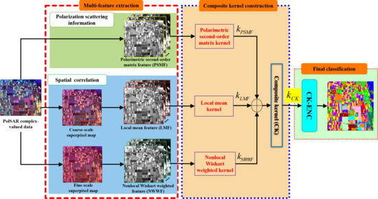
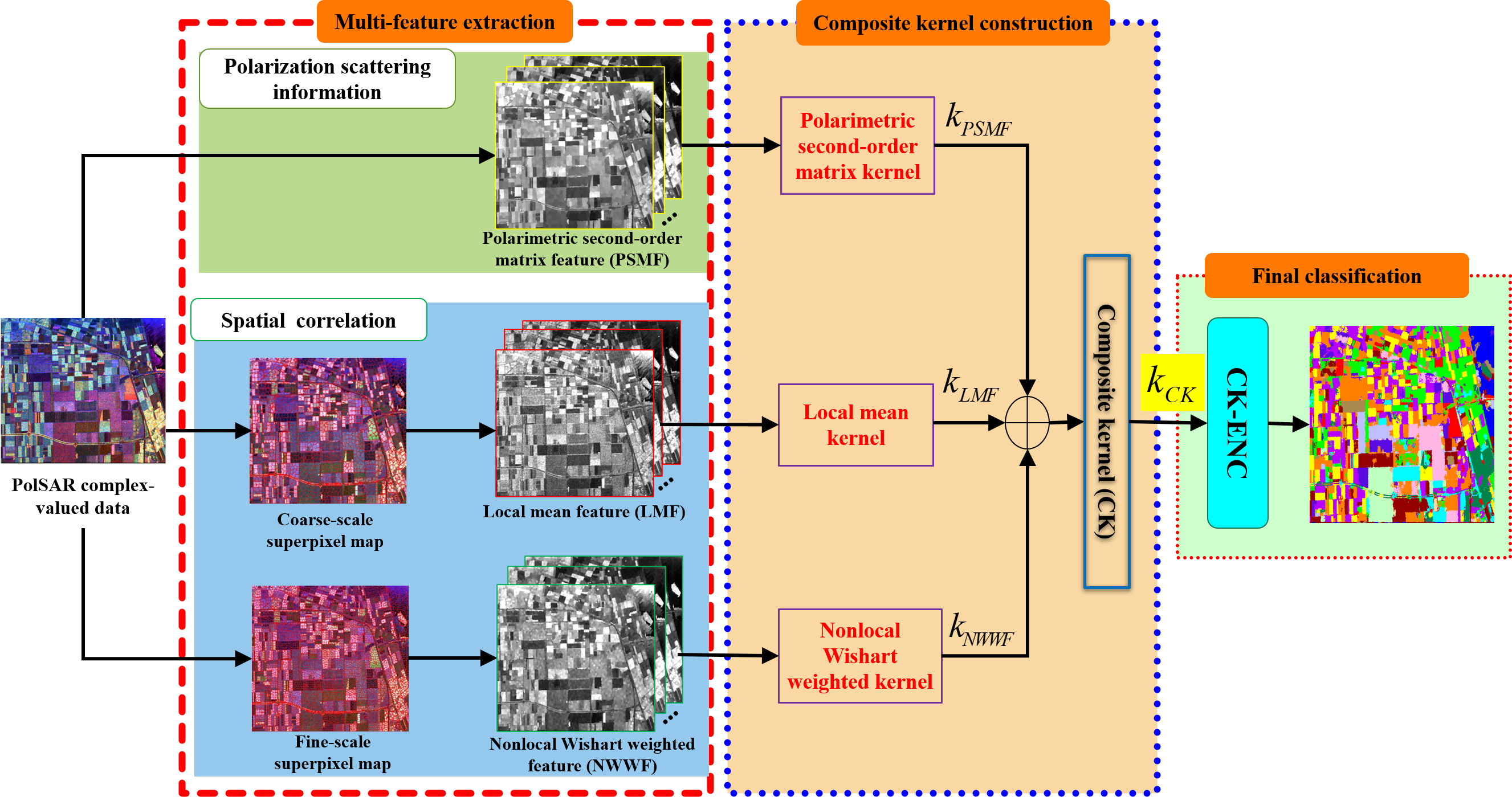
The flowchart of the proposed method is illustrated in Figure 1. It contains three modules, multi-feature extraction, CK construction for feature fusion, and CK-ENC for final PolSAR image classification.

2.1. Multi-Feature Extraction

To derive better and richer semantic representation, based on superpixel segmentation and statistical analysis, a multi-feature extraction strategy is proposed to extract three features for obtaining accurate classification results.

2.1.1. Polarimetric Second-Order Matrix Feature

To suppress the interference of speckles, as the second-order statistics, the polarimetric coherency matrix $\mathrm{T}$ is utilized to analyze the electromagnetic scattering characteristics of the distributed target [1]:

$$\begin{array}{c}\hfill \mathrm{T}=〈{\mathrm{u}}_L·{\mathrm{u}}_L^{\mathrm{H}}〉=\frac{1}{2}\left[\begin{array}{ccc}〈{\left|S_{HH}+S_{VV}\right|}^2〉& 〈\left(S_{HH}+S_{VV}\right){\left(S_{HH}-S_{VV}\right)}^{*}〉& 2〈\left(S_{HH}+S_{VV}\right)S_{HV}^{*}〉\\ 〈\left(S_{HH}-S_{VV}\right){\left(S_{HH}+S_{VV}\right)}^{*}〉& 〈{\left|S_{HH}-S_{VV}\right|}^2〉& 2〈\left(S_{HH}-S_{VV}\right)S_{HV}^{*}〉\\ 2〈S_{HV}{\left(S_{HH}+S_{VV}\right)}^{*}〉& 2〈S_{HV}{\left(S_{HH}-S_{VV}\right)}^{*}〉& 4〈{\left|S_{HV}\right|}^2〉\end{array}\right],\end{array}$$

(1)

where V denotes vertical polarization and H denotes horizontal polarization. $S_{HH},S_{HV},S_{VH}$, and $S_{VV}$ are four complex backscattered coefficients. ${\mathrm{u}}_L$ is the polarimetric target vector [1]. The superscript $\mathrm{H}$ denotes the conjugate transpose, and $\langle .\rangle$ indicates temporal or spatial ensemble averaging.

It is clear that $\mathrm{T}$ is an HPD matrix. This paper adopts $\mathrm{T}$ as the straightforward and effective polarimetric second-order matrix feature (PSMF) to describe each pixel in a PolSAR image. In other words, a $3\times 3\times H\times W$ polarimetric feature matrix based on $\mathrm{T}$ is utilized to describe the PolSAR image with a size of $H\times W$. This can avoid the problems caused by the explicit feature extraction and keep the contour information of targets in classification results.

2.1.2. Local Mean Feature within Coarse-Scale Superpixels

The coarse-scale superpixels are first generated by the modified SLIC algorithm [38] to consider the spatial relationship between pixels. Then, the local mean feature (LMF) of each pixel in a PolSAR image is extracted via the similarity within the superpixels.

Each superpixel is a disjoint and homogeneous pixel block, which can be regarded as a stationary and homogeneous area with uniform texture. In a homogeneous area with fully developed speckles and no texture, $\mathrm{T}$ obeys the complex Wishart distribution [47], i.e., $\mathrm{T}\sim W_{\mathrm{T}}\left(n,q,\mathbf{\Sigma }\right)$. Where the parameter q is 3 for monostatic PolSAR on a reciprocal medium, and n is the number of looks. $\mathbf{\Sigma }=\mathrm{E}\left\{\mathrm{T}\right\}$, and $Tr(.)$ is the trace of a matrix.

Assume that the ith pixel ${\mathrm{T}}_i$ in a PolSAR image belongs to the superpixel ${\mathrm{Y}}_k^{\mathrm{SP}}$. Let $\left\{{\mathrm{T}}_j\right\}$ be a group of adjacent pixels with similar properties within superpixel ${\mathrm{Y}}_k^{\mathrm{SP}}$, where $j=1,2,\dots ,J_k$, and $J_k$ is the number of pixels. Note that each superpixel represents a local, stationary region, ${\mathrm{T}}_i$ in superpixel ${\mathrm{Y}}_k^{\mathrm{SP}}$ can be modeled by a complex Wishart model, i.e., ${\mathrm{T}}_i\sim W_{{\mathrm{T}}_i}\left(n,q,{\widehat{\mathbf{\Sigma }}}_k^{\mathrm{SP}}\right)$. Thus, we estimate the statistical parameter ${\widehat{\mathbf{\Sigma }}}_k^{\mathrm{SP}}$ as the LMF to exploit spatial information. ${\widehat{\mathbf{\Sigma }}}_k^{\mathrm{SP}}$ is calculated with the maximum-likelihood (ML) estimator [47]:

$${\widehat{\mathbf{\Sigma }}}_k^{\mathrm{SP}}=\frac{1}{J_k}\sum _{j=1}^{J_k}{\mathrm{T}}_j.$$

(2)

Similar to the Equation (2), the LMF of each pixel can be extracted. Relying on coarse-scale superpixels, the local stationary information in a whole PolSAR image can be obtained to effectively suppress the influence of speckles and improve the visual coherence of the classification map.

2.1.3. Nonlocal Wishart Weighted Feature among Fine-Scale Superpixels

To obtain more accurate and robust classification performance, more descriptive and discriminative features should be extracted to provide additional invaluable information. Inspired by the nonlocal idea in [41], the nonlocal Wishart weighted feature (NWWF) is extracted. It can exploit the nonlocal spatial information around each superpixel, which can provide a richer spatial context to enhance the discriminability of each pixel.

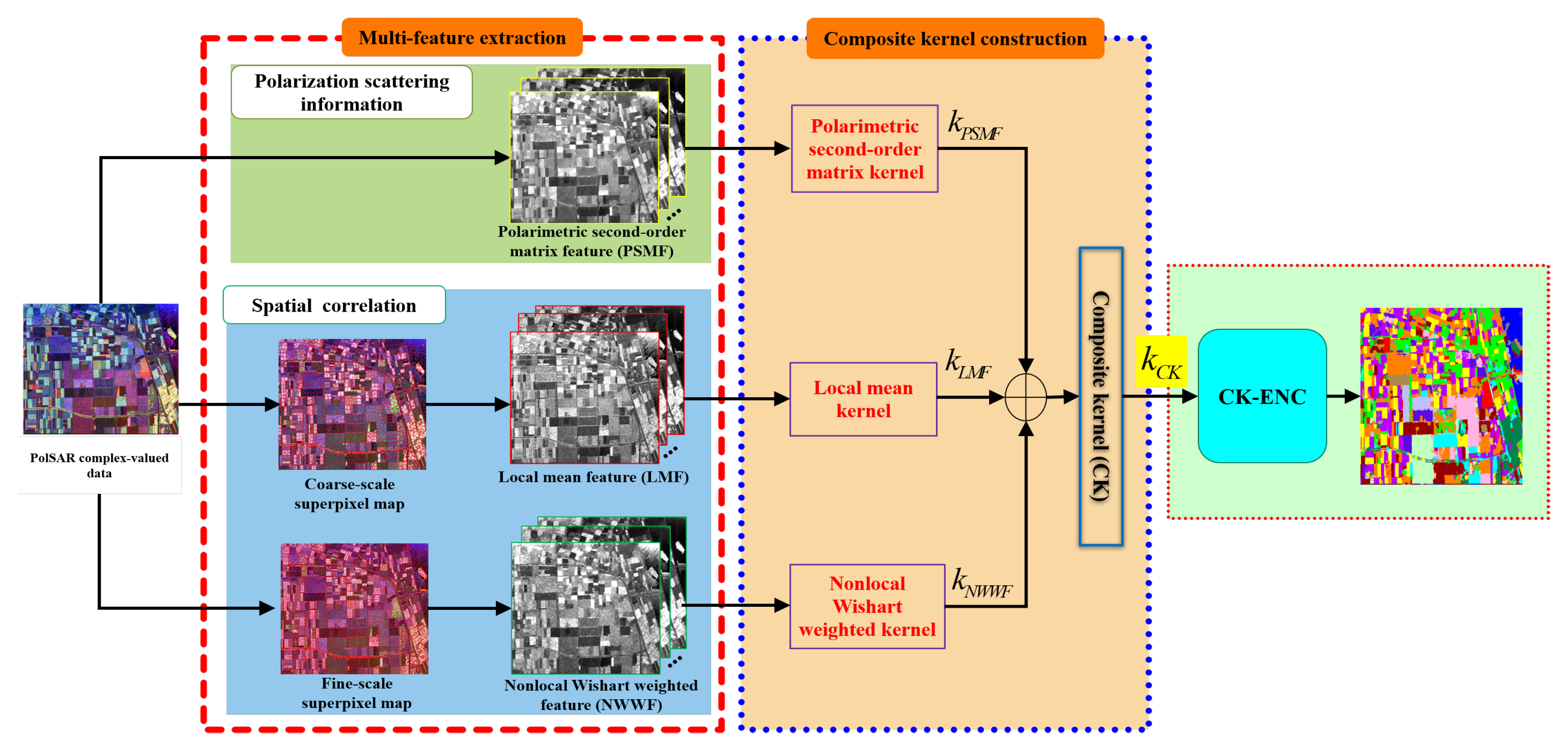
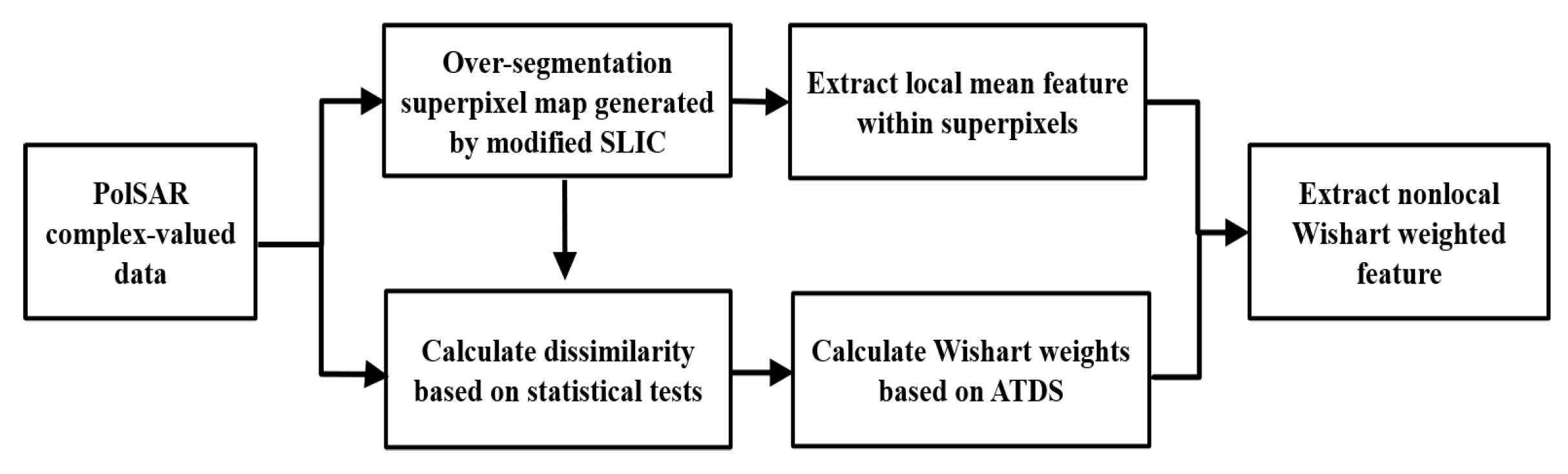
Figure 2 summarizes the main steps of NWWF extraction process. The key ingredient comes from the Wishart weight, which balances the relative importance of neighboring superpixels around the current superpixel.

Considering the robustness and computation efficiency, the distance derived from the Wishart test statistic is adapted for the dissimilarity measure between superpixels [37,47]. Let ${\mathbf{\Sigma }}_i^{\mathrm{SP}}$ and ${\mathbf{\Sigma }}_j^{\mathrm{SP}}$ respectively denote the center covariance matrix of superpixels ${\mathrm{Y}}_i^{\mathrm{SP}}$ and ${\mathrm{Y}}_j^{\mathrm{SP}}$, the dissimilarity distance between the ith and jth superpixels is defined as:

$$D_{\mathrm{S}}\left({\mathrm{Y}}_i^{\mathrm{SP}},{\mathrm{Y}}_j^{\mathrm{SP}}\right)=\left(N_i+N_j\right)ln\left|{\widehat{\mathbf{\Sigma }}}^{\mathrm{SP}}\right|-N_{i}ln\left|{\widehat{\mathbf{\Sigma }}}_i^{SP}\right|-N_{j}ln\left|{\widehat{\mathbf{\Sigma }}}_j^{\mathrm{SP}}\right|,$$

(3)

where ${\widehat{\mathbf{\Sigma }}}_i^{\mathrm{SP}}$ and ${\widehat{\mathbf{\Sigma }}}_j^{\mathrm{SP}}$ respectively are ML estimators of ${\mathbf{\Sigma }}_i^{\mathrm{SP}}$ and ${\mathbf{\Sigma }}_j^{\mathrm{SP}}$ in Equation (2). Details of the aforementioned derivation can be found in [37,47].

After the dissimilarity measurement, weights of neighborhood superpixels, which balances the relative importance, can be derived from the dissimilarity. For one superpixel ${\mathrm{Y}}_i^{\mathrm{SP}},$ all neighborhood superpixels can be denoted by $\left\{{\mathrm{Y}}_m^{\mathrm{SP}}\right\},$ where $m=1,2,\dots ,M,$ and M is the total number. Based on the distance $D_{\mathrm{S}}\left({\mathrm{Y}}_i^{\mathrm{SP}},{\mathrm{Y}}_m^{\mathrm{SP}}\right),$ the Wishart weight $w_{i,m}$ between ${\mathrm{Y}}_i^{\mathrm{SP}}$ and ${\mathrm{Y}}_m^{\mathrm{SP}}$ can be estimated by the exponential kernel:

$$w_{i,m}=exp\left(-\gamma D_{\mathrm{S}}^2\left({\mathrm{Y}}_i^{\mathrm{SP}},{\mathrm{Y}}_m^{\mathrm{SP}}\right)\right),$$

(4)

where $\gamma$ is the scale parameter. If the center superpixel ${\mathrm{Y}}_i^{\mathrm{SP}}$ and a neighborhood superpixel ${\mathrm{Y}}_m^{\mathrm{SP}}$ are more similar, the value of weight $w_{i,m}$ will be higher.

Notably, there may be some neighborhood superpixels belonging to the different categories with the center superpixel, which still make a contribution by weights for the final NWWF extraction. This will make results disturbed by heterogeneous regions with smaller weights. Therefore, to improve the robustness to heterogeneous, a more effective weight computation is adopted as follows:

$$w_{i,m}=\left\{\begin{array}{cc}exp\left(-\gamma D_{\mathrm{S}}^2\left({\mathrm{Y}}_i^{\mathrm{SP}},{\mathrm{Y}}_m^{\mathrm{SP}}\right)\right),& D_{\mathrm{S}}\left({\mathrm{Y}}_i^{\mathrm{SP}},{\mathrm{Y}}_m^{\mathrm{SP}}\right)<\tau \\ 0,& \mathrm{otherwise}\end{array}\right.,$$

(5)

where $\tau$ is the adaptive threshold, which is provided by an AIDS. Inspired by [42], we extend AIDS to deal with PolSAR images. Assume a PolSAR image contains C classes, the set of available training samples can be denoted as $\mathrm{X}=\left[{\mathrm{X}}^1,{\mathrm{X}}^2,\dots ,{\mathrm{X}}^C\right]$ with C subsets. Each subset ${\mathrm{X}}^c=\left[{\mathrm{T}}_1^c,{\mathrm{T}}_2^c\dots ,{\mathrm{T}}_{n_c}^c\right]\in {\mathbb{R}}^{3\times 3\times n_c}$ is constructed by $n_c$ training samples in the class $c(c=1,2,\dots ,C).$ The total number of all training samples for the training set is N and $N={\sum }_{c=1}^C{n}_c.$ For the cth class, the mean coherency matrix is calculated as:

$${\mathrm{T}}^c=\frac{1}{n_c}\sum _{k=1}^{n_c}{\mathrm{T}}_k^c.$$

(6)

According to Equation (3), all distances between two classes can be computed, which can be composed the set $\left\{D_1,D_2,\dots ,D_{C(C-1)/2}\right\}$ in ascending order. Then, we take the median values in this set as the adaptive threshold $\tau$ to decide weights:

$$\tau =median\left\{D_1,D_2,\dots ,D_{C(C-1)/2}\right\}.$$

(7)

Based on dissimilarity and threshold decided by AIDS, the new weight computation scheme can reduce or even eliminate the impact of the heterogeneous regions, thereby improving the representation performance.

Finally, with the calculated weights, the NWWF of pixels in superpixel ${\mathrm{Y}}_i^{\mathrm{SP}}$ can be estimated in a weighted maximum likelihood way:

$${\widehat{\mathbf{\Sigma }}}_i^{\mathrm{NWWF}}=\frac{{\sum }_{m=1}^M{w}_{i,m}·{\widehat{\mathbf{\Sigma }}}_m^{\mathrm{SP}}}{{\sum }_{m=1}^M{w}_{i,m}}.$$

(8)

It is worth noting that, to preserve more details and achieve relatively good performance, superpixels with the fine-scale size are generated to extract local mean spatial features for Equation (8). In other words, compared with Equation (2), the local spatial feature ${\widehat{\mathbf{\Sigma }}}_m^{\mathrm{SP}}$ in Equation (8) is generated by superpixels with different size.

In summary, for each pixel in a PolSAR image, three features are extracted to preserve the original CV attributes, suppress the interference of speckles, and capture more discriminative information to obtain more accurate classification results.

2.2. Composite Kernel (CK) Construction

The above three extracted features for each pixel all $3\times 3$ CV matrices, which form a nonlinear manifold. This nonlinear geometry often makes PolSAR classification complicated and difficult. Therefore, to better build a classifier for PolSAR images, a composite kernel (CK) is developed based on geometric distance and kernel method. It can map these features to the Hilbert space and realize the multi-feature information fusion to achieve promising classification accuracy.

On the Riemannian manifold, the similarities between points can be measured by the geodesic distance [36]. The widely used geodesic distances include the affine invariant Riemannian metric (AIRM) [36], the log-Euclidean distance (LED) [48], and the Bartlett distance [49]. Due to the eigenvalue decomposition in the equation, AIRM has high computational complexity [27]. In addition, LED applies the Euclidean metric by projecting the SPD matrix into the Euclidean space, which distorts the matrix structure and may lead to suboptimal results [28]. Rather than the eigenvalue decomposition for AIRM, the Bartlett distance only needs to calculate the matrix logarithm operation, which means a low computational load. Therefore, for simple calculation and effective implementation, this paper chooses the Bartlett distance.

Given two SPD matrices $\mathrm{X}\in {\mathbb{C}}^{p\times p}$ and $\mathrm{Y}\in {\mathbb{C}}^{p\times p}$ on a Riemannian manifold, the Bartlett distance, also known as Stein divergence or Jensen-Bregman LogDet divergence, is defined as:

$$d_{\mathrm{Bartlett}}(\mathrm{X},\mathrm{Y})=log\left|\frac{\mathrm{X}+\mathrm{Y}}{2}\right|-\frac{log\left|\mathrm{XY}\right|}{2},$$

(9)

where $log(·)$ is the principal matrix logarithm.

In addition, through the kernel method, matrices on the Riemannian manifold can be embedded into the RKHS to handle the nonlinearity. In this way, many pattern recognition methods can be utilized for the PolSAR image classification. Base on the Gaussian RBF kernel and the above Bartlett distance, the Stein kernel function [28] can be defined as:

$$k_{\mathrm{Stein}}(\mathrm{X},\mathrm{Y})=exp\left(-\beta d_{\mathrm{Bartlett}}(\mathrm{X},\mathrm{Y})\right)=2^{p\beta }\frac{\sqrt{{\left|\mathrm{X}\right|}^{\beta }{\left|\mathrm{Y}\right|}^{\beta }}}{{|\mathrm{X}+\mathrm{Y}|}^{\beta }}.$$

(10)

The Stein kernel is a positive definite kernel when the values of $\beta$ is inside of the following set:

$$\beta \in \left\{\frac{1}{2},\frac{2}{2},\dots ,\frac{p-1}{2}\right\}\cup \left\{\tau \in \mathbb{R}:\tau >\frac{p-1}{2}\right\}.$$

(11)

In this paper, the choice of $\beta$ is $(p-1)/2$.

Therefore, according to the stein kernel, three features are mapped into the RKHS to form three different kernels, and then the CK is composed of the three kernels. More specifically, given the polarimetric second-order matrix feature ${\mathrm{X}}_s^{\mathrm{PSMF}}\in {\mathbb{C}}^{p\times p}$ for the pixel $s=\{i,j\},$ the mapped polarimetirc second-order matrix kernel, dented by $k_{\mathrm{PSMF}}\left({\mathrm{X}}_i,{\mathrm{X}}_j\right)$, is defined as:

$$\begin{array}{c}\hfill k_{\mathrm{PSMF}}\left({\mathrm{X}}_i,{\mathrm{X}}_j\right)=exp\left(-\beta d_{\mathrm{Bartlett}}\left({\mathrm{X}}_i^{\mathrm{PSMF}},{\mathrm{X}}_j^{\mathrm{PSMF}}\right)\right)=2^{p\beta }\frac{\sqrt{{\left|{\mathrm{X}}_i^{\mathrm{PSMF}}\right|}^{\beta }{\left|{\mathrm{X}}_j^{\mathrm{PSMF}}\right|}^{\beta }}}{{\left|{\mathrm{X}}_i^{\mathrm{PSMF}}+{\mathrm{X}}_j^{\mathrm{PSMF}}\right|}^{\beta }}\end{array}.$$

(12)

For the local mean feature denoted by ${\mathrm{X}}_s^{\mathrm{LMF}}\in {\mathbb{C}}^{p\times p},$ the mapped local mean kernel $k_{\mathrm{LMF}}\left({\mathrm{X}}_i,{\mathrm{X}}_j\right)$ is as follows:

$$k_{\mathrm{LMF}}\left({\mathrm{X}}_i,{\mathrm{X}}_j\right)=exp\left(-\beta d_{\mathrm{Bartlett}}\left({\mathrm{X}}_i^{\mathrm{LMF}},{\mathrm{X}}_j^{\mathrm{LMF}}\right)\right).$$

(13)

In addition, similarlu to Equation (13), the nonlocal Wishart weighted kernel $k_{\mathrm{NWWF}}\left({\mathrm{X}}_i,{\mathrm{X}}_j\right)$ mapped from the nonlocal Wishart weighted feature ${\mathrm{X}}_s^{\mathrm{NWWF}}\in {\mathbb{C}}^{p\times p}$ is calculated as:

$$k_{\mathrm{NWWF}}\left({\mathrm{X}}_i,{\mathrm{X}}_j\right)=exp\left(-\beta d_{\mathrm{Bartlett}}\left({\mathrm{X}}_i^{\mathrm{NWWF}},{\mathrm{X}}_j^{\mathrm{NWWF}}\right)\right).$$

(14)

Finally, according to the properties of Mercer’s kernels [43], the CK can be created by combing the above three kernels:

$$\begin{array}{c}\hfill k_{\mathrm{CK}}\left({\mathrm{X}}_i,{\mathrm{X}}_j\right)={\mu }_{\mathrm{PSMF}}.k_{\mathrm{PSMF}}\left({\mathrm{X}}_i,{\mathrm{X}}_j\right)+{\mu }_{\mathrm{LMF}}.k_{\mathrm{LMF}}\left({\mathrm{X}}_i,{\mathrm{X}}_j\right)+{\mu }_{\mathrm{NWWF}}.k_{\mathrm{NWWF}}\left({\mathrm{X}}_i,{\mathrm{X}}_j\right)\end{array},$$

(15)

where ${\mu }_{\mathrm{PSMF}},{\mu }_{\mathrm{LMF}}$, and ${\mu }_{\mathrm{NWWF}}$ are the weight parameters of the three different kernels. Their values are satisfied:

$${\mu }_{\mathrm{PSMF}}+{\mu }_{\mathrm{LMF}}+{\mu }_{\mathrm{NWWF}}=1,{\mu }_{\mathrm{PSMF}},{\mu }_{\mathrm{LMF}},{\mu }_{\mathrm{NWWF}}\in [0,1].$$

(16)

For the proposed CK-ENC, the three weights ${\mu }_{\mathrm{PSMF}},{\mu }_{\mathrm{LMF}}$, and ${\mu }_{\mathrm{NWWF}}$ are set to 0.1, 0.2, and 0.7, respectively. In the following experimental part, the influences of these weights on the performances of the proposed method will be further analyzed.

2.3. Composite Kernel-Based Elastic Net Classifier (CK-ENC)

For higher computational efficiency and better classification accuracy, the CK integrated with the ENC is developed for the PolSAR image classification. Under the condition of few training samples, ENC can estimate robust coefficients to reveal a more powerful discriminant ability for better classification performance.

For a testing sample $y\in {\mathbb{C}}^{p\times p},$ the objection of ENC is to find the coefficient vector $\alpha \in {\mathbb{R}}^{n\times 1}$ for the linear combination of the training samples $\mathrm{X}=\left[{\mathrm{X}}^1,{\mathrm{X}}^2,\dots ,{\mathrm{X}}^C\right]$ with the combination of ${\ell }_1$ and ${\ell }_2$ penalties. Thus, the objective function under the kernel framework can be formulated as:

$$\begin{array}{c}\hfill \widehat{\alpha }=arg{\displaystyle \underset{\alpha }{min}}\frac{1}{2}{∥\varphi \left(y\right)-{\displaystyle \sum _{c=1}^c}\varphi \left({\mathrm{X}}^c\right){\alpha }^c∥}_2^2+{\lambda }_1{\parallel \alpha \parallel }_1+{\lambda }_2{\parallel \alpha \parallel }_2^2\end{array},$$

(17)

where ${\lambda }_1$ and ${\lambda }_2$ are the regularization parameters. $\varphi (.)$ is an embedding function, which maps the data from Riemannian manifold into PKHS. $\alpha =\left[{\alpha }^1,\dots ,{\alpha }^c,\dots ,{\alpha }^c\right]$ is the coefficient vector to reconstruct the testing sample $\mathrm{y},$ and ${\alpha }^c\in {\mathbb{R}}^{n_c\times 1}$ is the vector representing coefficients corresponding to the subset ${\mathrm{X}}^c.$ It is known that the inner product of two instances in PKHS can be calculated by a kernel function $k(.):\langle \varphi \left(\mathrm{A}\right),\varphi \left(\mathrm{B}\right)\rangle =k(\mathrm{A},\mathrm{B}),$ where $\mathrm{A}$ and $\mathrm{B}$ are all on a Riemannian manifold. Thus, Equation (17) can be expanded as:

$$\begin{array}{c}\hfill \widehat{\alpha }=arg\underset{\alpha }{min}\frac{1}{2}\left(k(y,y)-2\sum _{c=1}^c{\alpha }^c·k\left({\mathrm{X}}^c,y\right)+\sum _{i,j=1}^c{\alpha }^i{\alpha }^j·k\left({\mathrm{X}}^i,{\mathrm{X}}^i\right)\right)+{\lambda }_1{\parallel \alpha \parallel }_1+{\lambda }_2{\parallel \alpha \parallel }_2^2\end{array}.$$

(18)

In this paper, the objective function in Equation (18) adopts the CK in Equation (15). In addition, the sparse modeling software [50] is used to solve the convex problem in Equation (18) and find the optimized solution $\widehat{\alpha }=\left[{\widehat{\alpha }}^1,\dots ,{\widehat{\alpha }}^c,\dots ,{\widehat{\alpha }}^c\right]$. According to the estimated coefficient vector $\widehat{\alpha },$ the testing sample y can be classified to the best category by the following rule:

$$class\left(y\right)=arg\underset{c=1,\dots ,C}{min}\frac{{∥y-{\mathrm{X}}^c{\widehat{\alpha }}^c∥}_2}{{∥{\widehat{\alpha }}^c∥}_2}.$$

(19)

In the same way, the classification of a complete PolSAR image can be realized. In summary, we propose the CK-ENC to achieve pixel-level PolSAR classification. CK-ENC makes good use of the inherent statistical characteristics and the spatial information of PolSAR data through the CK. Thus, it can obtain more discriminative representation and overcome the influence of speckles, thereby preserving image boundaries well and making the classification results smoother. In addition, under the condition of limited training samples, the CK-ENC combines the CK with ENC to achieve PolSAR image classification, which can balance the between-class interference and within-class variations to obtain more accurate classification results. Subsequently, we will investigate the effectiveness of the proposed CK-ENC method with real PolSAR images.

3. Experimental Results

Experiments were carried out to evaluate the classification capability of the proposed CK-ENC method. We first introduce three real PolSAR datasets utilized in the experiments and three objective metrics for quantitative evaluation of classification performance. Then, a comparison to classification algorithms and the experimental setup are given. Finally, to make a sufficient comparison among various algorithms, the visualized classification results and the quantitative performance are displayed for the full demonstration.

3.1. Experimental Datasets Description and Objective Metrics

To demonstrate the effectiveness of CK-ENC, we select three real PolSAR datasets from an airborne system (L-band AIRSAR) and two spaceborne systems (C-band GaoFen3 and C-band RADARSAT-2). The three selected PolSAR pseudo-images are from different areas, and the types and quantities of classes in these datasets are also different. Therefore, the effectiveness of the proposed classification method can be verified by three selected datasets in terms of the system, the operative band, and the classification problem. The details of these datasets are listed as following.

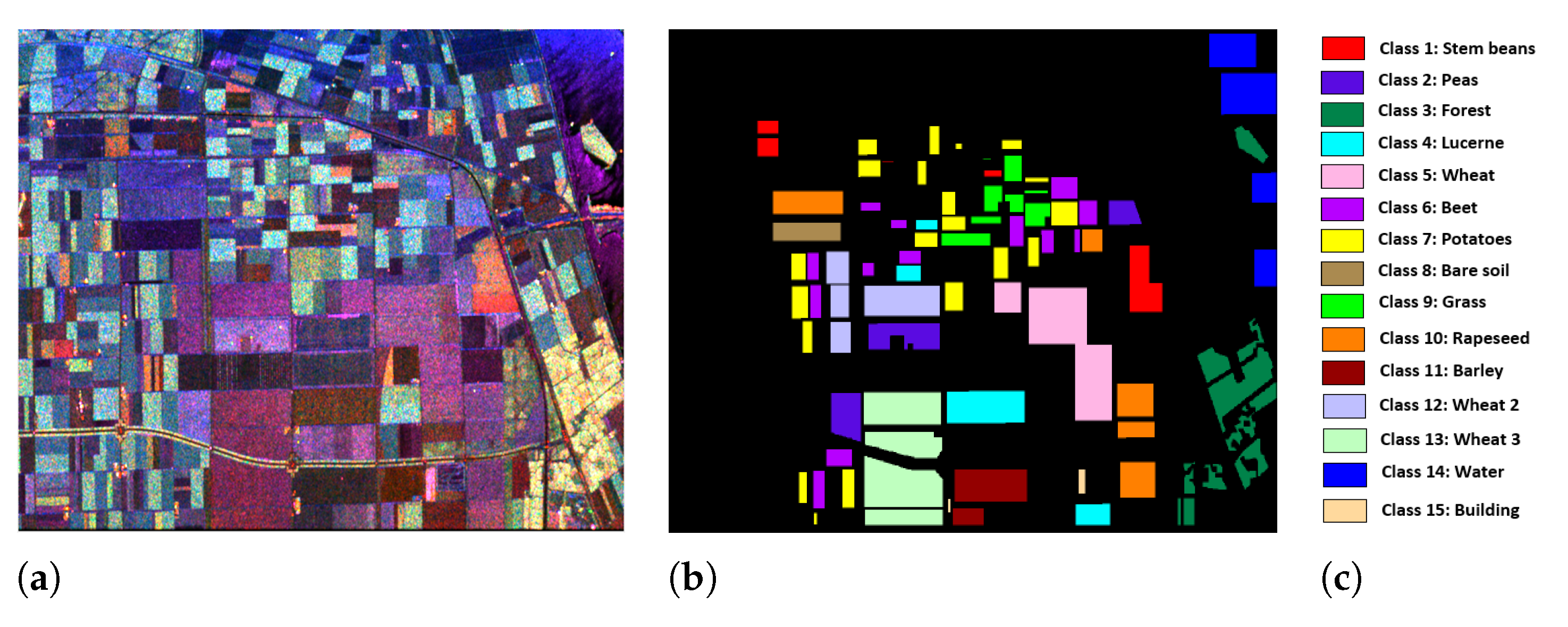
3.1.1. Flevoland Benchmark Dataset

It is an L-band four-look PolSAR data with a size of 750 × 1024 pixels, acquired by the NASA/JPL AIRSAR system on August 16, 1989. The Pauli RGB image is shown in Figure 3a and contains 15 classes: stem beans, peas, forest, lucerne, wheat, beet, potatoes, bare soil, grass, rapeseed, barley, wheat2, wheat3, water, buildings. The ground-truth of the image is shown in Figure 3b, and the corresponding color code is displayed in Figure 3c.

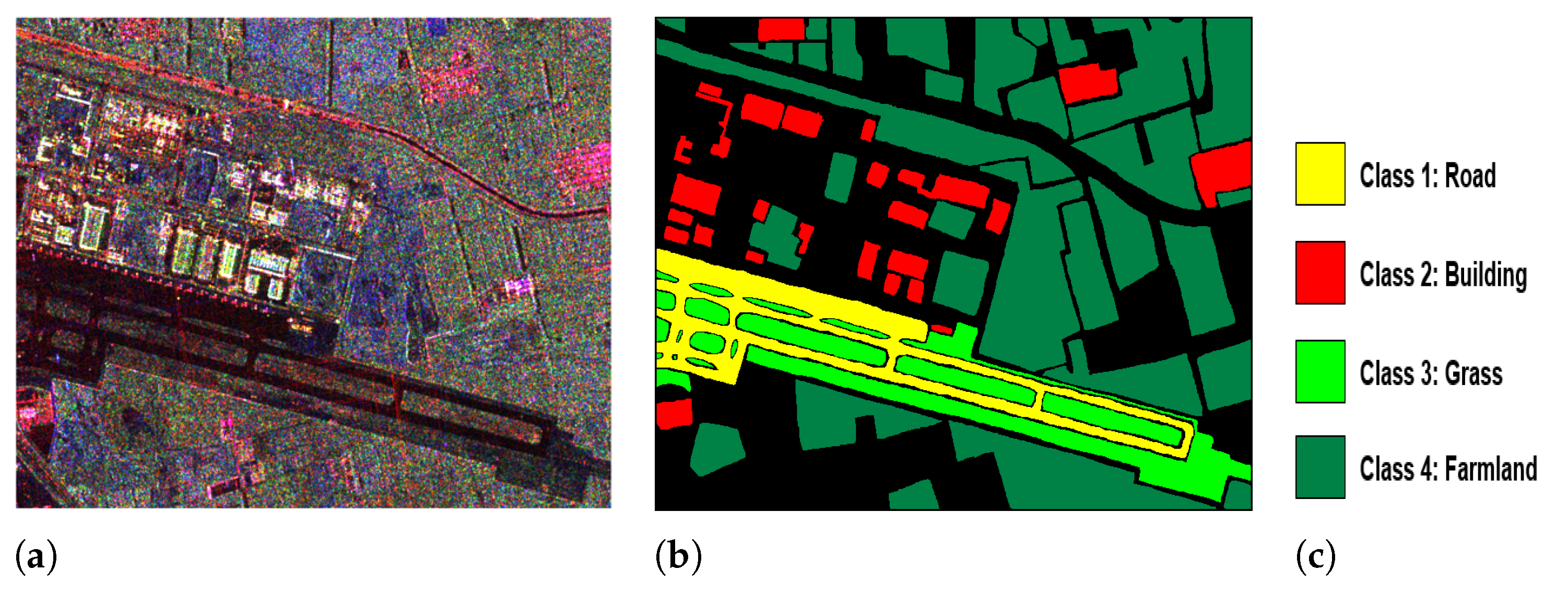
3.1.2. Yihechang Dataset

The Yihechang dataset near a domestic airport in China was obtained by the spaceborne GaoFen3 system of the China National Space Administration (CNSA) in 27 June 2019. The Pauli RGB map are shown in Figure 4a. As a fully polarized image of the C-band, its image size is 590 × 800 pixels, and the resolution is 5m. This dataset is provided by the Aerospace Information Research Institute, Chinese Academy of Sciences. There are four land cover classes identified in this dataset: road, building, grass, and farmland. Figure 4b,c show the ground truth and the corresponding color code, respectively.

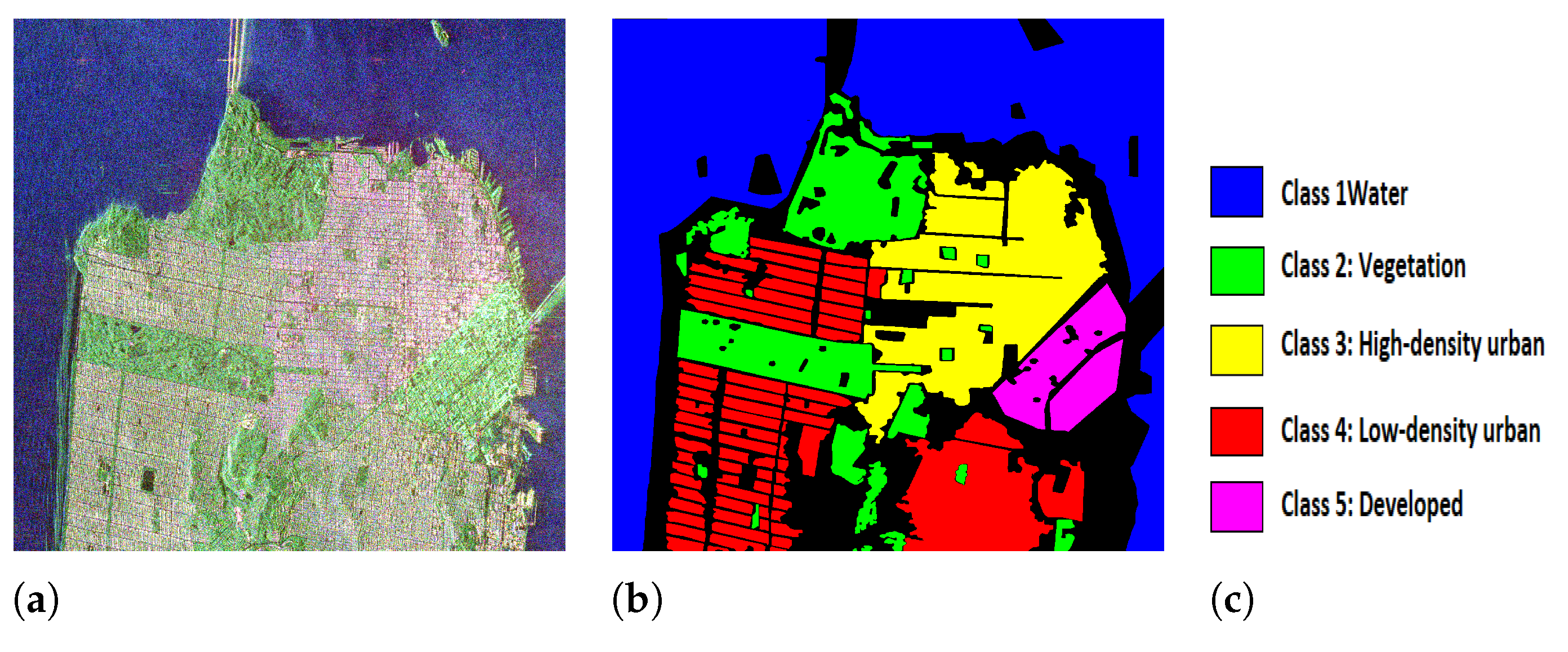
3.1.3. San Francisco Dataset

The third dataset, San Francisco, is obtained by RADARSAT-2 in 9 April 2008, which is a spaceborne system of the Canadian Space Agency. It is the C-band full PolSAR image and is composed of 1800 × 1380 pixels. The Pauli RGB image, the ground-truth map, and the color code are respectively shown in Figure 5a–c. The image consists of five major classes: water, vegetation, high-density urban, low-density urban, and developed.

To evaluate the quantitative performance of different algorithms, three objective metrics are adopted, namely, overall accuracy (OA), average accuracy (AA), and the Kappa coefficient ($\kappa$). Besides, the individual accuracy (CA) of each class is also listed. Specifically, OA refers to the percentage of correctly classified testing samples in all testing samples; AA is the mean of all class accuracies; Kappa is a robustness measurement with the degree of agreement.

3.2. Comparison Algorithms and Experimental Setup

To verify the effectiveness of the proposed method, the proposed CK-ENC is compared with some competing methods including Wishart-based ML (WML) [23], region-based Markov random field (RMRF) [39], random forest (RF) [2], support vector machine (SVM) [6], multilayer projective dictionary pair learning and sparse autoencoder-based method (MDPL-SAE) [10], adaptive nonlocal stacked sparse autoencoder (ANSSAE) [11], SRC with majority voting (SRC-MV) [51], superpixel-based joint SRC (JSRC-SP) [51], Wishart-based joint CRC (W-JCRC) [52], and double kernels SRC (DK-SRC) [28]. In this paper, it is not our main purpose to examine the impact of spatial information on classification results. Therefore, for the WML and RF methods, the spatial information is introduced into these methods by superpixel-based segmentation. They are denoted by S-WML and S-RF, respectively. In addition, we found that the classifiers with the explicit feature-based kernels gain poor classification performance under the condition of limited training samples. Thus, for a fair comparison, we replace these kernels in SRC-MV, JSRC-SP, and W-JCRC methods with the polarimetric second-order statistical kernel. Since the proposed method combines the CK, we construct the CK-SVM classifier according to [6] for testing. The optimization problem of CK-SVM is resolved by the LIBSVM library [53] and the parameters are obtained by cross-validation. In addition, the CK is embedded into CRC and SRC separately to compare the performance of representation-based classifiers. For deep learning-based methods MDPL-SAE and ANSSAE, their parameters are tuned by cross-validation. In this paper, the MDPL-SAE and ANSSAE are implemented in the Keras framework with TensorFlow as the backend. Other methods are all run on MATLAB R2014a. The machine used for experiments is a Lenovo Y720 cube gaming PC with an Intel Core i7-7700 CPU, an Nvidia GeForce GTX 1080 GPU, and 16GB RAM under Ubuntu 18.04 LTS operating system.

For the proposed CK-ENC, we conduct experiments to set the number of superpixels and the regularization parameters ${\lambda }_1$ and ${\lambda }_2$. It should be noted that the number of superpixels is decided by the initial expected spatial size R for similar pixels search [51]. Thus, we vary the value of R to observe its impact on the classification results. To explore the effect of these parameters on the performance of CK-ENC and tune them, we utilize the leave-one-out cross validation (LOOCV) strategy to conduct the experiments based on available training samples. In addition, the same training and testing samples are chosen in the same set of experiments to ensure consistency [46]. The labeled samples of each dataset were divided into training and test sets randomly. For all datasets, 20 labeled pixels per class are randomly chosen for training, and the remaining labeled samples are treated as the test set. To avoid any bias, the experimental results are repeated ten times, and the mean OA values are reported.

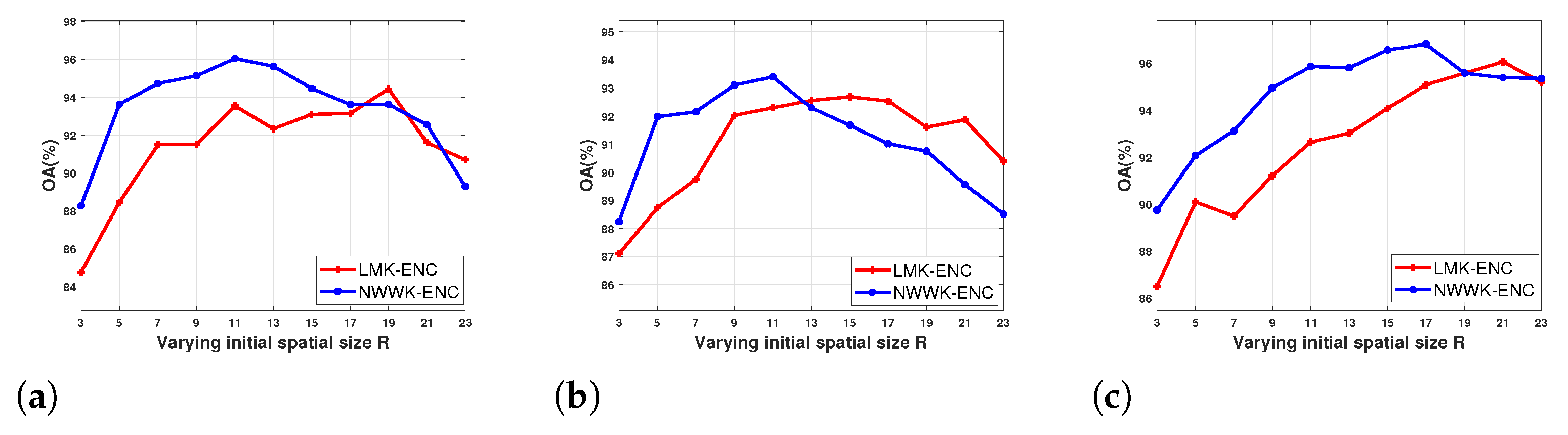
3.2.1. Impact of the Number of Superpixels

We first report experiments about the influence of the number of superpixels on the classification performance. According to the previous theory, the local mean kernel $k_{\mathrm{LMF}}$ and the nonlocal Wishart weighted kernel $k_{\mathrm{NWWF}}$ are all affected by the number of superpixels. Thus, for all datasets, the ENC with the $k_{\mathrm{LMF}}$ (LMK-ENC) and the $k_{\mathrm{NWWF}}$ (NWWK-ENC) are respectively employed to determine the optimal number of superpixels. As mentioned above, the optimal number of superpixels means the optimal R. Here, the value of R ranges from 3 to 23, and the interval is 2. Figure 6 illustrates the OA values of the two classifiers under the varying initial spatial sizes. It can be observed that the classification accuracies of LMK-ENC and NWWK-ENC are all worse when the value of R is small. With the increase of R value, the OA curve shows a trend of first increasing and then decreasing. In addition, for three datasets, the optimal R values of NWWK-ENC are all smaller than the optimal value of LMK-ENC. This can be explained as follows. If the value of R is too much smaller, each superpixel may not provide enough spatial information for accurate classification. On the other hand, a much larger value of R may cause more heterogeneous pixels to be contained in each superpixel, which easily leads to insufficient segmentation. Moreover, for NWWK-ENC, the smaller value of R than LMK-ENC can alleviate the effect of heterogeneous pixels. At the same time, enough spatial information is provided through the weighted neighborhood superpixels. Based on the above analysis and the results in Figure 6, the R parameters of LMK-ENC and NWWK-ENC for different datasets are set according to their best performances. The details of the R parameters settings are shown in

Table 1. Detailed R settings for different datasets.

Dataset	LMK-ENC	NWWK-ENC
Flevoland	19	11
Yihechang	15	11
San Francisco	21	17

.

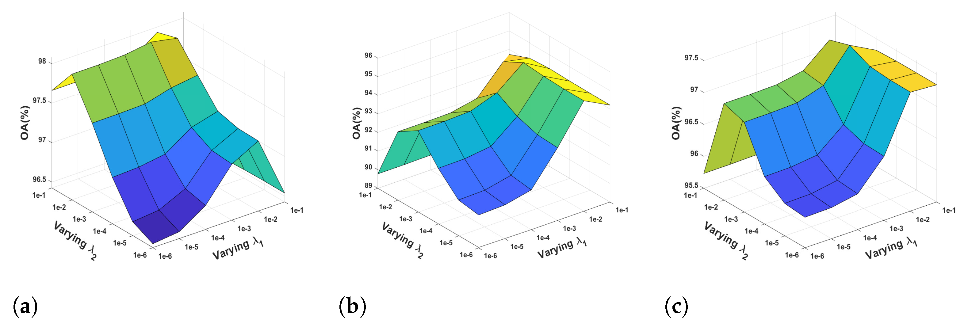
3.2.2. Impact of the Regularization Parameters

The regularization parameters ${\lambda }_1$ and ${\lambda }_2$ are critical for the proposed CK-ENC, which are used to balance the data item and the penalty items. On the one hand, too much smaller values of ${\lambda }_1$ and ${\lambda }_2$ have no contribution to higher overall classification accuracy. On the other hand, when the values of ${\lambda }_1$ and ${\lambda }_2$ exceed a threshold, too many important features may be lost, resulting in reduced classification accuracy. To search the optimal regularization parameters ${\lambda }_1$ and ${\lambda }_2$ for the experimental datasets, we conduct experiments in the range of ${\lambda }_1=1e-6,1e-5,\dots ,1e-1$ and ${\lambda }_2=1e-6,1e-5,\dots ,1e-1$. Figure 7 demonstrates the results on the three PolSAR datasets. As shown in Figure 7, when ${\lambda }_1=1e-2$ and ${\lambda }_2=1e-3$, the performance of CK-ENC for the Flevoland is the best. For the Yihechang and San Francisco, the best regularization parameters ${\lambda }_1$ and ${\lambda }_2$ are $1e-3$ and $1e-2,$ respectively.

3.3. Classification Results Comparison

In this sub-section, we evaluate the effectiveness of the proposed PolSAR image classification method by the visualized classification results and the quantitative performance.

3.3.1. Experiment on Flevoland Dataset

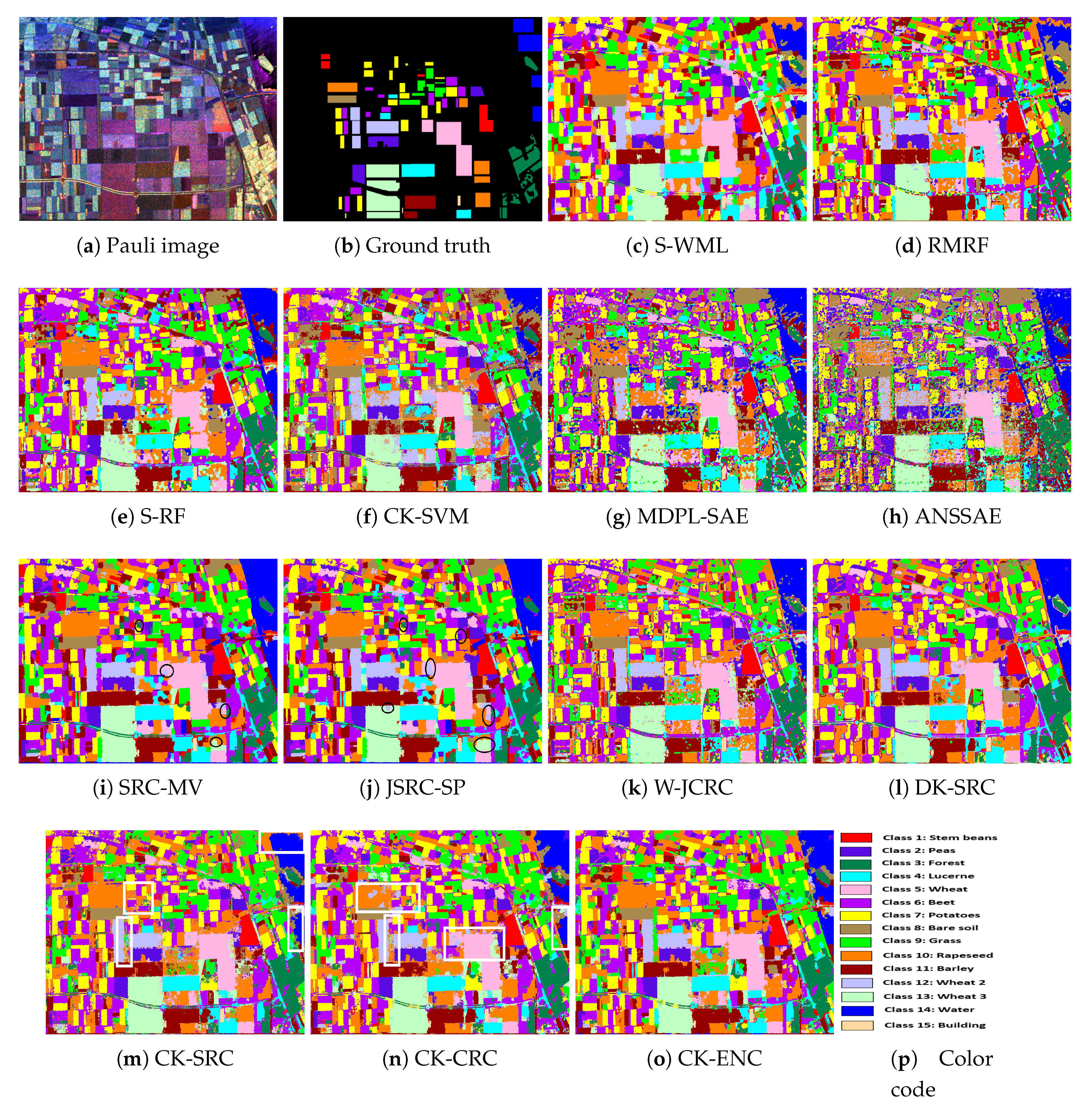
The first experiment is carried on the Flevoland dataset. The classification accuracies of different algorithms are shown in

Table 2. Comparision of classification performances on the Flevoland dataset.

Class	S-WML	RMRF	S-RF	CK-SVM	MDPL-SAE	ANSSAE	SRC-MV	JSRC-SP	W-JCRC	DK-SRC	CK-SRC	CK-CRC	CK-ENC
1	98.28 ± 0.06	99.59 ± 0.07	99.39 ± 0.03	99.62 ± 0.11	95.74 ± 0.26	94.49 ± 0.56	99.69 ± 0.11	99.69 ± 0.17	99.47 ± 0.08	99.15 ± 0.25	99.74 ± 0.02	96.00 ± 0.78	99.47 ± 0.01
2	89.81 ± 1.71	99.64 ± 0.11	98.92 ± 0.19	99.68 ± 0.19	94.23 ± 0.80	93.47 ± 0.86	99.69 ± 0.02	99.69 ± 0.01	99.08 ± 0.20	99.43 ± 0.28	99.68 ± 0.01	99.90 ± 0.16	99.67 ± 0.03
3	94.93 ± 1.46	93.49 ± 1.01	98.55 ± 0.65	98.14 ± 0.29	95.68 ± 1.07	90.44 ± 0.51	97.94 ± 0.38	98.10 ± 0.27	96.62 ± 0.71	99.23 ± 0.30	99.06 ± 0.58	97.79 ± 0.45	99.18 ± 0.54
4	92.64 ± 0.66	98.86 ± 1.30	96.45 ± 1.06	99.86 ± 0.02	89.51 ± 1.55	93.66 ± 1.26	96.73 ± 1.78	99.57 ± 0.15	99.23 ± 0.30	97.83 ± 0.57	96.95 ± 0.79	97.99 ± 0.73	99.08 ± 0.02
5	86.24 ± 1.12	88.07 ± 1.20	83.98 ± 1.98	85.45 ± 1.39	97.41 ± 0.29	88.18 ± 0.50	96.66 ± 1.28	94.06 ± 0.94	92.68 ± 1.58	95.04 ± 0.55	97.32 ± 0.62	94.29 ± 1.58	98.11 ± 0.16
6	95.60 ± 0.21	97.79 ± 1.25	99.49 ± 0.28	99.41 ± 0.05	92.21 ± 0.57	70.79 ± 1.24	96.92 ± 0.53	94.10 ± 0.40	98.81 ± 0.71	97.62 ± 0.21	98.60 ± 0.18	98.75 ± 0.19	98.98 ± 0.01
7	98.27 ± 0.81	96.95 ± 0.95	98.20 ± 0.50	99.27 ± 0.07	87.42 ± 0.84	85.29 ± 1.01	93.69 ± 1.49	91.66 ± 0.55	95.25 ± 0.21	98.74 ± 0.47	99.46 ± 0.24	99.41 ± 0.36	99.18 ± 0.14
8	97.78 ± 1.28	94.98 ± 0.54	100 ± 0	100 ± 0	99.38 ± 0.48	98.86 ± 0.13	100 ± 0	100 ± 0	99.87 ± 0.06	99.22 ± 0.05	97.97 ± 0.17	97.98 ± 1.16	99.80 ± 0.01
9	87.99 ± 1.94	74.87 ± 1.66	95.26 ± 0.52	74.75 ± 2.46	90.91 ± 0.63	82.66 ± 0.37	99.86 ± 0.05	99.86 ± 0.26	92.75 ± 0.88	92.70 ± 1.43	96.53 ± 0.44	95.13 ± 1.45	96.14 ± 0.15
10	84.34 ± 0.42	78.24 ± 0.56	90.30 ± 0.18	64.30 ± 2.49	74.67 ± 2.22	65.20 ± 1.65	76.10 ± 2.16	70.96 ± 1.48	85.14 ± 1.67	93.67 ± 0.94	92.75 ± 0.60	89.86 ± 1.29	93.91 ± 0.22
11	91.91 ± 0.59	99.23 ± 0.03	97.51 ± 0.48	99.66 ± 0.03	92.10 ± 0.18	95.56 ± 1.16	99.15 ± 0.49	99.15 ± 0.43	94.91 ± 0.79	95.20 ± 0.91	99.08 ± 0.06	97.05 ± 1.91	98.88 ± 0.36
12	95.95 ± 0.41	97.89 ± 1.10	91.62 ± 0.92	84.77 ± 1.45	50.91 ± 1.78	80.36 ± 0.93	97.64 ± 0.99	97.64 ± 0.08	95.56 ± 1.05	98.97 ± 0.24	98.98 ± 0.46	96.13 ± 0.51	95.18 ± 1.10
13	94.51 ± 0.96	95.61 ± 0.97	91.48 ± 1.12	92.51 ± 0.74	94.99 ± 0.45	94.43 ± 0.45	99.32 ± 0.22	98.06 ± 0.30	98.23 ± 1.05	99.02 ± 0.03	98.31 ± 0.67	97.33 ± 1.21	99.01 ± 0.68
14	69.27 ± 1.14	49.41 ± 1.27	91.23 ± 0.07	50.81 ± 2.64	81.97 ± 1.83	88.62 ± 0.46	100 ± 0	100 ± 0	99.11 ± 0.43	99.93 ± 0.02	99.55 ± 0.31	97.79 ± 1.24	98.34 ± 0.86
15	98.71 ± 0.12	92.70 ± 0.87	99.16 ± 0.45	98.42 ± 0.02	94.54 ± 0.32	97.90 ± 0.26	99.12 ± 0.12	99.12 ± 0.12	96.71 ± 0.32	98.93 ± 0.58	81.36 ± 1.45	98.93 ± 0.18	98.46 ± 0.04
OA	90.65 ± 0.85	89.54 ± 0.29	94.04 ± 0.10	87.83 ± 0.36	88.13 ± 0.89	86.74 ± 0.59	96.21 ± 0.65	95.11 ± 0.54	95.94 ± 0.33	97.66 ± 0.32	98.06 ± 0.05	97.05 ± 0.27	98.18 ± 0.09
AA	91.75 ± 0.54	90.49 ± 0.25	93.50 ± 0.03	89.65 ± 0.35	88.78 ± 1.17	87.99 ± 0.52	96.83 ± 0.12	96.11 ± 0.43	96.29 ± 0.25	96.64 ± 0.39	97.02 ± 0.64	97.20 ± 0.84	98.23 ± 0.17
$\mathit{\kappa }\times$ 100	89.91 ± 0.92	88.62 ± 0.32	95.31 ± 0.11	86.76 ± 0.39	87.05 ± 0.96	85.55 ± 0.64	95.86 ± 0.71	94.66 ± 0.60	95.56 ± 0.35	97.45 ± 0.35	97.89 ± 0.39	96.79 ± 0.30	98.01 ± 0.01

, and the comparison results are shown in Figure 8.

From Table 2, it is apparent that the proposed CK-ENC performs better than other compared methods, in terms of OA, AA, and the Kappa coefficient. Compared with S-WML and RMRF, CK-ENC obtains higher accuracies with a more than 8% improvement in OA. That clearly demonstrates the advantage of capsuling more discriminative features. By utilizing more effective features, S-RF can achieve a better classification result. However, it cannot maintain a balance between different classes. As presented in this table, although the OA of the Bare soil reaches 100%, the OA of the Wheat is only 83%. This phenomenon also appears in CK-SVM, MDPL-SAE, and ANSSAE. The main reason may be that due to the limitation of available labeled samples, the training-based classification algorithms cannot fully explore and learn the inherent polarimetric information. Thus, they cannot identify all classes effectively to maintain a classification balance between classes. For SRC-MV and JSRC-SP based on superpixels, they can achieve classification accuracies than 95%. Additionally, W-JCRC based on the statistical distance-weighted regularization obtains an OA up to 95.94%. However, none of them consider nonlocal spatial information, which results in accuracy lower than CK-ENC. By considering the nonlocal spatial information, the OA of DK-SRC reaches 97.66%. It indicates that it is necessary to introduce nonlocal spatial information for more accurate classification results. Although DK-SRC achieves a great classification result, its performance is not as good as the proposed CK-ENC. Compared with DK-SRC, CK-ENC improves the accuracy of wheat, grass, and barley by about 4%. It may be the result of the integration of more spatial information and the fusion of various types of features. In addition, the results of CK-ENC are better than CK-SRC and CK-CRC, which illustrates that ENC combining ${\ell }_1$ and ${\ell }_2$-norm regularized terms outperforms the original SRC and CRC. Overall, for the Flevoland dataset, the proposed CK-ENC achieves the best classification accuracy, especially when the number of labeled samples is limited.

As shown in Figure 8, the proposed CK-ENC performs a better visual effect than other methods and has better agreement with the ground truth. As shown in Figure 8c–e, S-WML and RMRF misclassify a considerably large part of water into bare soil. S-RF achieves a bad result in recognizing wheat3, but it can distinguish water well. As shown in Figure 8f–h, the classification maps by training-based methods have many notable misclassified pixels, which is consistent with the results listed in Table 2. It indicates that the proposed CK-ENC can provide competitive performance even with limited labeled samples. Comparing Figure 8o with Figure 8i,j, the proposed CK-ENC can reduce the number of misclassified homogeneous regions (as highlighted by black ovals). This illustrates that fusing pixel-based features (i.e., PSMF) and capturing more discriminant information is indispensable to improve classification results. From Figure 8k,l, we can see that the classification maps are over-smoothed, and the pixels located around class boundaries are misclassified. The reason is that W-JCRC and DK-SRC utilize rectangle windows to joint neighboring pixels. By contrast, CK-ENC adopts superpixels to provide adaptive spatial information, thereby avoiding mixing pixels belonging to different classes and preserving image boundaries well. In addition, compared with Figure 8m,n, CK-ENC can obtain a better and accurate classification result (as highlighted by white rectangles). According to Table 2 and Figure 8, it can be concluded that the proposed CK-ENC outperforms other compared approaches on the Flevoland dataset.

3.3.2. Experiment on Yihechang Dataset

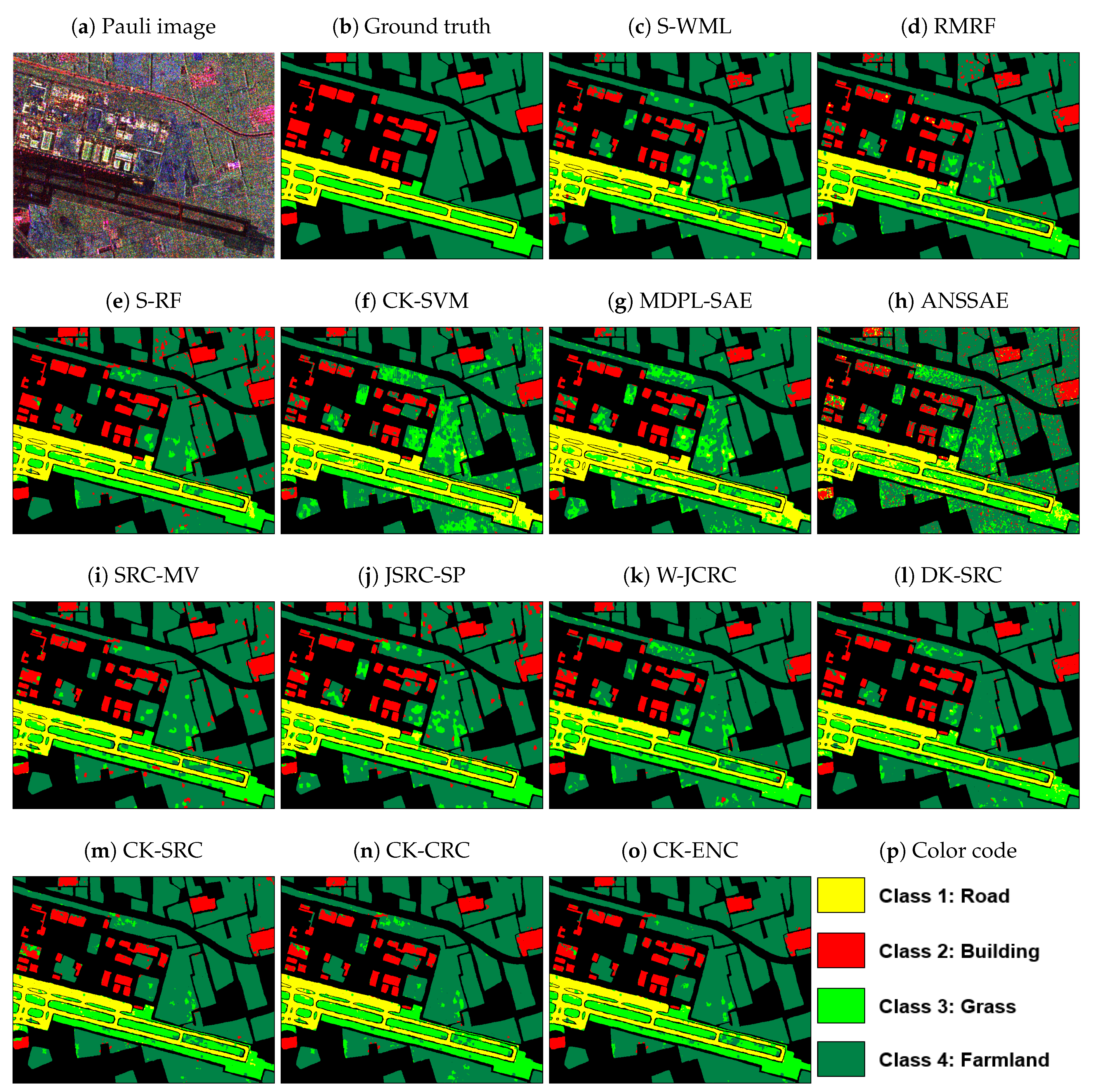
The second experiment is conducted on the Yihechang dataset. The quantitative evaluation results are listed in

Table 3. Comparision of classification performances on the Yihechang dataset.

Class	S-WML	RMRF	S-RF	CK-SVM	MDPL-SAE	ANSSAE	SRC-MV	JSRC-SP	W-JCRC	DK-SRC	CK-SRC	CK-CRC	CK-ENC
1	92.86 ± 0.78	91.04 ± 0.21	97.04 ± 0.41	96.44 ± 0.74	98.04 ± 0.79	97.03 ± 0.43	91.61 ± 0.79	92.12 ± 0.87	79.45 ± 2.12	89.03 ± 1.60	95.00 ± 0.25	91.90 ± 1.29	92.64 ± 0.75
2	71.62 ± 1.59	78.60 ± 2.63	96.47 ± 0.25	79.17 ± 2.41	81.79 ± 1.09	72.18 ± 1.62	89.68 ± 1.24	92.70 ± 0.27	87.25 ± 1.78	92.11 ± 0.70	89.67 ± 0.80	91.31 ± 0.56	92.82 ± 0.56
3	80.75 ± 1.08	81.41 ± 1.53	84.57 ± 1.99	65.53 ± 2.15	48.28 ± 3.57	69.78 ± 2.70	84.65 ± 1.75	90.50 ± 1.75	91.27 ± 0.80	87.09 ± 1.63	90.66 ± 1.35	93.60 ± 1.28	92.44 ± 1.19
4	96.02 ± 0.95	96.17 ± 0.49	90.89 ± 0.27	80.51 ± 1.23	88.11 ± 0.76	82.61 ± 1.37	94.97 ± 0.18	89.85 ± 1.94	94.84 ± 0.27	96.31 ± 0.47	97.83 ± 0.73	97.22 ± 0.59	98.48 ± 0.63
OA	90.91 ± 1.07	91.64 ± 0.54	91.33 ± 0.39	80.14 ± 0.88	83.07 ± 0.98	81.38 ± 1.20	92.58 ± 0.36	90.51 ± 1.17	91.75 ± 0.97	93.74 ± 0.76	95.63 ± 0.26	95.47 ± 0.26	96.36 ± 0.22
AA	85.31 ± 1.28	86.81 ± 1.17	92.24 ± 0.26	80.41 ± 0.91	79.06 ± 1.22	80.40 ± 0.28	90.23 ± 0.43	91.29 ± 0.94	88.20 ± 1.74	91.14 ± 0.57	93.29 ± 0.27	93.51 ± 0.17	94.10 ± 0.44
$\mathit{\kappa }\times$ 100	83.20 ± 1.42	84.48 ± 0.88	84.93 ± 0.58	66.90 ± 0.89	70.60 ± 1.71	68.38 ± 1.69	86.59 ± 0.69	85.53 ± 1.85	85.08 ± 1.74	88.64 ± 1.31	92.02 ± 0.44	91.77 ± 0.46	93.34 ± 0.38

, and the classification maps are shown in Figure 9.

As shown in Table 3, the proposed CK-ENC has the highest accuracy and kappa coefficient. What is more, compared with other methods, CK-ENC has excellent performance for correctly classifying the Farmland. That shows that our method can provide more discriminant information by the multi-feature fusion, thereby achieving satisfying results for complex scattering classes. As shown in Figure 9, the classification map of CK-ENC has fewer remarkable misclassified pixels and is much clearer and smoother compared with other methods. Moreover, CK-ENC significantly reduces the misclassification of the edges and improves the visual coherence of the classification map. Therefore, for the Yihechang dataset, whether objective metrics or visual performance, the proposed CK-ENC delivers better performance than other compared methods.

3.3.3. Experiment on San Francisco Dataset

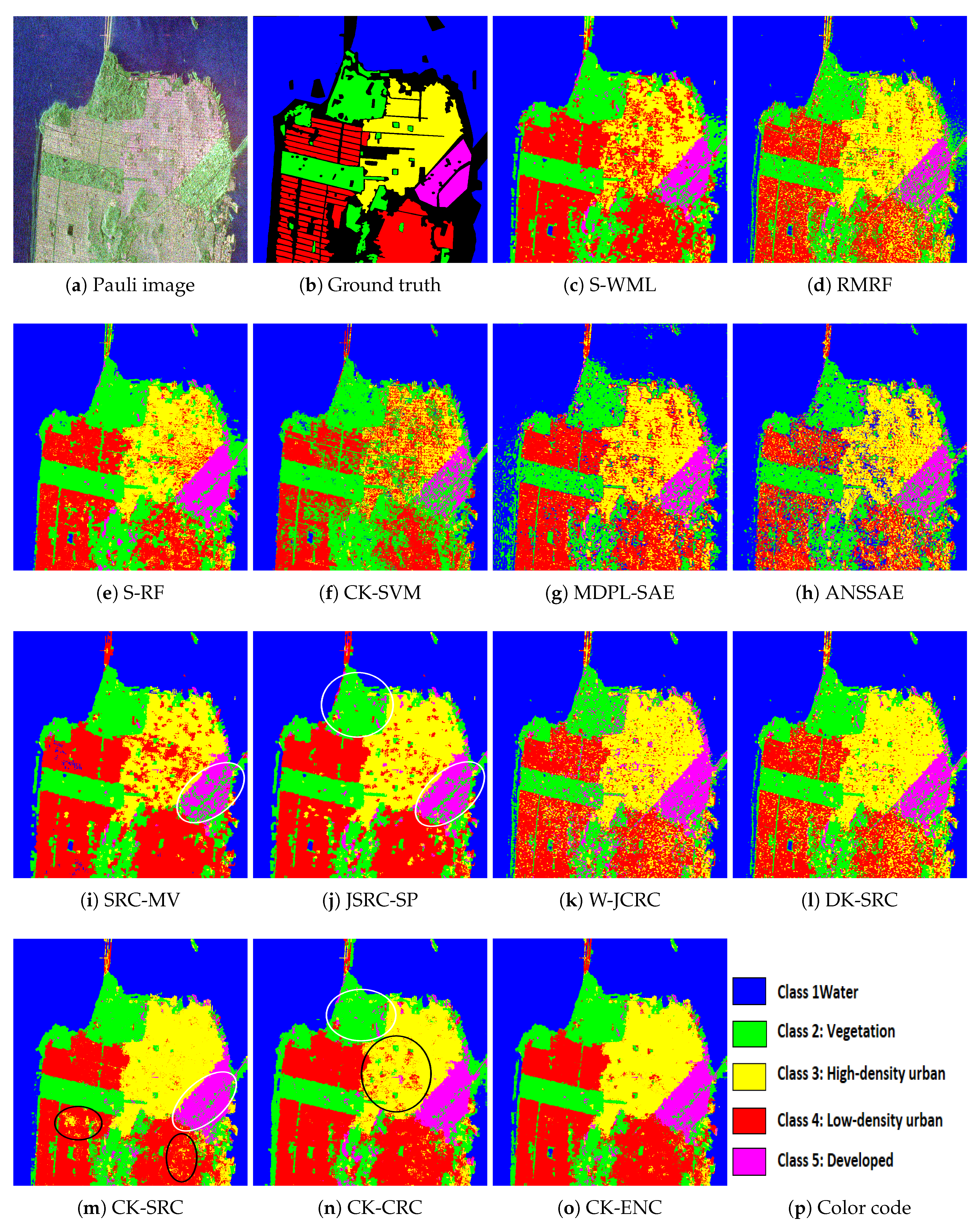
The third experiment is conducted on the San Francisco dataset.

Table 4. Comparision of classification performances on the San Franciso dataset.

Class	S-WML	RMRF	S-RF	CK-SVM	MDPL-SAE	ANSSAE	SRC-MV	JSRC-SP	W-JCRC	DK-SRC	CK-SRC	CK-CRC	CK-ENC
1	98.11 ± 0.85	99.15 ± 0.23	99.03 ± 0.04	100 ± 0	95.61 ± 0.76	99.69 ± 0.24	99.99 ± 0.01	99.96 ± 0.02	99.91 ± 0.05	99.96 ± 0.04	99.98 ± 0.08	99.47 ± 0.27	99.95 ± 0.01
2	90.88 ± 1.16	88.62 ± 1.09	94.83 ± 1.13	93.75 ± 0.88	84.80 ± 1.47	86.41 ± 1.54	92.80 ± 0.53	90.85 ± 0.98	82.87 ± 1.70	90.87 ± 1.42	92.85 ± 1.47	89.26 ± 1.15	92.03 ± 0.98
3	65.20 ± 2.94	83.92 ± 1.89	79.23 ± 2.07	43.69 ± 2.10	77.92 ± 0.09	76.25 ± 0.93	74.76 ± 1.94	89.67 ± 1.43	90.07 ± 0.46	93.08 ± 0.63	98.13 ± 0.48	92.74 ± 1.47	97.27 ± 0.64
4	92.20 ± 1.05	73.84 ± 2.27	84.25 ± 1.67	72.06 ± 0.94	83.29 ± 2.42	58.91 ± 0.91	96.73 ± 1.14	96.03 ± 1.16	78.56 ± 1.87	77.40 ± 2.16	92.79 ± 1.59	97.05 ± 1.48	96.16 ± 0.02
5	80.05 ± 1.75	69.78 ± 0.67	92.33 ± 0.40	58.97 ± 1.31	79.56 ± 0.22	74.24 ± 1.15	73.66 ± 1.54	84.25 ± 1.80	89.60 ± 0.74	83.33 ± 1.59	92.76 ± 1.50	95.54 ± 0.72	96.41 ± 0.47
OA	90.04 ± 1.28	89.14 ± 0.92	92.20 ± 0.39	83.07 ± 0.44	88.30 ± 1.42	85.19 ± 1.32	93.27 ± 0.10	95.68 ± 0.48	91.51 ± 1.10	92.55 ± 1.11	97.03 ± 0.33	96.43 ± 0.49	97.59 ± 0.24
AA	85.29 ± 1.81	83.06 ± 1.11	89.93 ± 1.19	73.69 ± 0.56	84.23 ± 0.40	79.10 ± 2.15	87.59 ± 1.56	92.15 ± 1.63	88.20 ± 1.00	88.93 ± 1.48	95.30 ± 0.51	94.82 ± 0.21	96.36 ± 0.40
$\mathit{\kappa }\times$ 100	85.69 ± 0.81	84.41 ± 1.33	88.80 ± 0.34	75.57 ± 0.60	83.16 ± 0.53	78.30 ± 0.83	90.28 ± 0.30	93.78 ± 0.21	87.83 ± 1.55	89.30 ± 0.59	95.73 ± 0.47	94.87 ± 0.70	96.54 ± 0.35

reports the quantitative evaluation results for different classification methods. The corresponding classification results are shown in Figure 10.

As shown in Table 4, CK-ENC has the highest OA value and Kappa coefficient, which demonstrates the effectiveness of the proposed method. Moreover, the AA value of CK-ENC is the highest, which proves that our method can extract features with the representation and discrimination ability, thereby maintaining the classification balance between classes. It is noteworthy that, for all urban classes including High-density urban, Low-density urban, and Developed, the CK-ENC yields accuracies more than 95%. This shows that even for similar classes with small differences, the proposed method also well captures within-class variation to present a better performance, which outperforms other competitive methods.

From Figure 10, it is apparent that CK-ENC performs the best visual effect. As shown in Figure 10c–l, serious confusions exist between high-density urban and low-density urban. This phenomenon has been weakened in Figure 10m–o, which indicates that the proposed CK can capsule more discriminant information by the feature fusion and eliminate the between-class interference. In addition, compared with Figure 10m,n, the proposed CK-ENC further alleviate this problem (as highlighted by black ovals), which is coincident with the results in Table 4. Moreover, for Developed and Vegetation, CK-ENC shows better visual effects in regional label consistency than other methods (as highlighted by white ovals). In summary, by the fusion of various types of features, the proposed CK-ENC method can captive more discriminative information, thereby exploring more characteristics contained in PolSAR data to obtain more accurate classification results.

4. Discussion

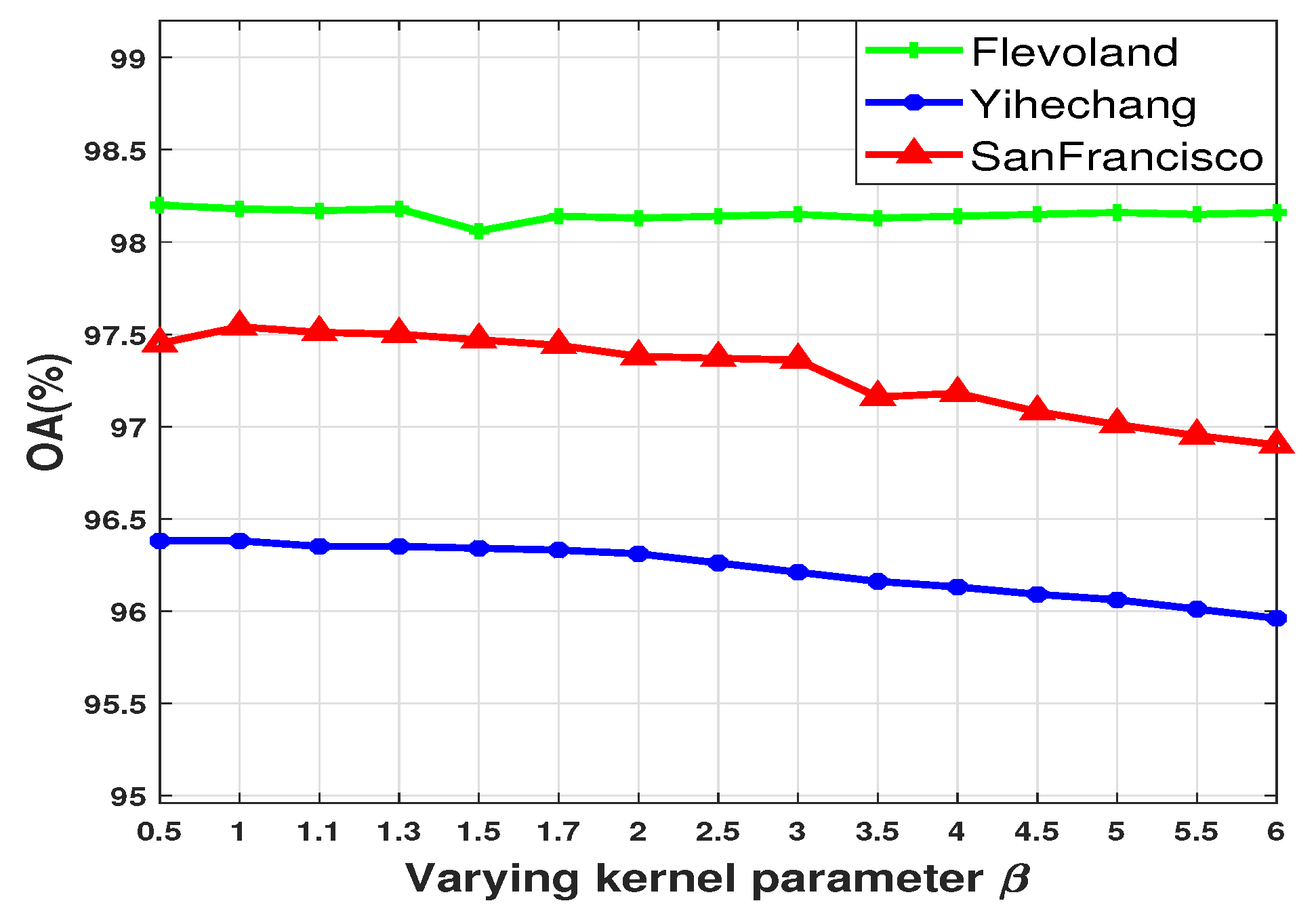
4.1. Impact of the Kernel Parameter $\beta$

To verify the influence of $\beta$ on the classification result, we select 15 values within the effective range of $\beta$ for experiments. Figure 11 illustrates the OA values of the proposed method under different $\beta$ values on the three PolSAR datasets. As shown in Figure 11, the change of $\beta$ value has little effect on classification performance. Therefore, without loss of generality, we set $\beta$ to $(p-1)/2$ in the above experiments, that is, $\beta =1$.

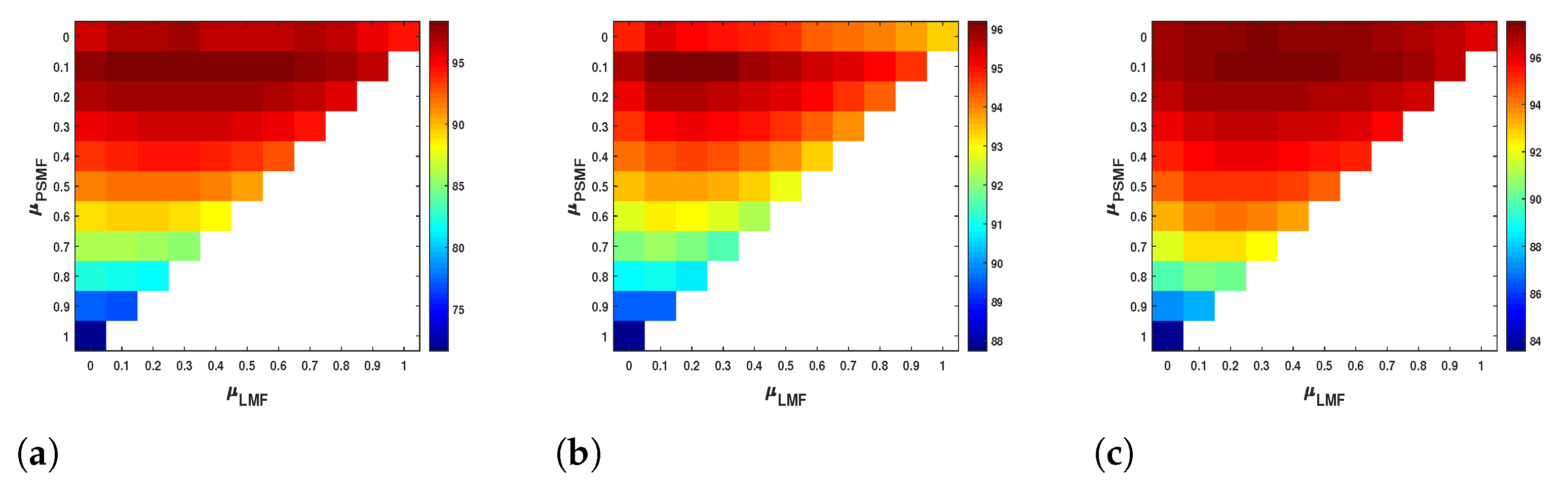
4.2. Impact of the Proposed Composite Kernel

In CK-ENC, the three kernel weights ${\mu }_{\mathrm{PSMF}}$, ${\mu }_{\mathrm{LMF}}$, and ${\mu }_{\mathrm{NWWF}}$ can reflect the contribution of the three feature kernels $k_{\mathrm{PSMF}}$, $k_{\mathrm{LMF}}$, and $k_{\mathrm{NWWF}}$ for classification. To verify the performance of the proposed CK $k_{\mathrm{CK}}$, Figure 12 illustrates the OA values of different combinations of kernel weight parameters ${\mu }_{\mathrm{PSMF}}$ and ${\mu }_{\mathrm{LMF}}$ under the condition of ${\mu }_{\mathrm{PSMF}}+{\mu }_{\mathrm{LMF}}+{\mu }_{\mathrm{NWWF}}=1$.

For the Flevoland dataset, when the three feature kernel are used separately, that is, when ${\mu }_{\mathrm{PSMF}}=1,{\mu }_{\mathrm{LMF}}=0,{\mu }_{\mathrm{NWWF}}=0$, the OA value is 71.61%, when ${\mu }_{\mathrm{PSMF}}=0,{\mu }_{\mathrm{LMF}}=1,{\mu }_{\mathrm{NWWF}}=0$, the OA value is 89.50%, and when ${\mu }_{\mathrm{PSMF}}=0,{\mu }_{\mathrm{LMF}}=0,{\mu }_{\mathrm{NWWF}}=1$, the OA value is 96.01%. Obviously, the OA value obtained by using only the $k_{\mathrm{PSMF}}$ is the lowest. This shows that the local mean feature (LMF) and the nonlocal Wishart weighted feature (NWWF) seem to be more effective for higher accuracy than the polarimetric second-order matrix feature (PSMF). When the $k_{\mathrm{PSMF}}$ is separately combined with $k_{\mathrm{LMF}}$ and $k_{\mathrm{NWWF}}$, i.e., $0<{\mu }_{\mathrm{PSMF}}<1,{\mu }_{\mathrm{NWWF}}=0$ and $0<{\mu }_{\mathrm{PSMF}}<1,{\mu }_{\mathrm{LMF}}=0$, the OA value increases first and then decreases. Especially when ${\mu }_{\mathrm{PSMF}}$ varies from 0.2 to 0.9, the OA value keeps decreasing. This indicates that NWWF should be utilized for the PolSAR image classification, but its weight value is comparatively smaller than other features. Therefore, this paper fixes the value of ${\mu }_{\mathrm{PSMF}}$ to 0.1 for three datasets. If the $k_{\mathrm{LMF}}$ and $k_{\mathrm{NWWF}}$ are used at the same time, i.e., ${\mu }_{\mathrm{PSMF}}=0$, with the increasing of ${\mu }_{\mathrm{LMF}}$, the change of OA value is to increase first and then decrease. The best OA value is 97.10%, which is higher than using both kernels alone. This shows that a suitable combination of LMF and NWWF has a positive impact on classification performance. From Figure 12a, we can observe that the highest OA value occurs when the three kernels are fused, i.e., ${\mu }_{\mathrm{PSMF}}\ne 0,{\mu }_{\mathrm{LMF}}\ne 0,{\mu }_{\mathrm{NWWF}}\ne 0$. This means the validity of the proposed composite kernel $k_{\mathrm{CK}}$.

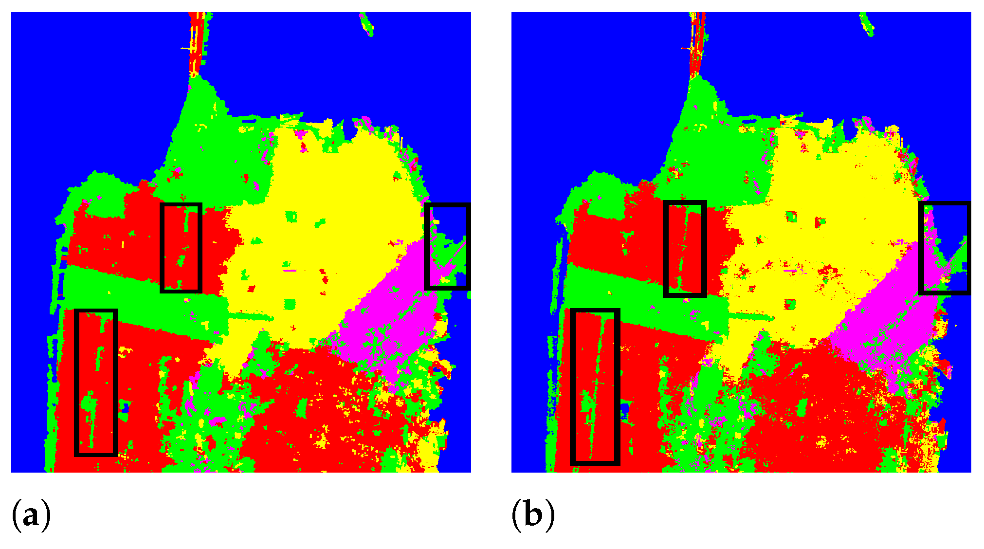
For the Yihechang and San Francisco datasets, it can be observed that the best classification results are obtained using CK. In addition, for the San Francisco dataset, although the increase in OA is not obvious when combining with the $k_{\mathrm{PSMF}}$, the contour details of some ground targets are clearer due to the fusion of PSMF. For better interpretation, Figure 13a,b respectively show the classification results without and with the $k_{\mathrm{PSMF}}$. As shown in Figure 13, the proposed method with the $k_{\mathrm{PSMF}}$ can identify the fine structures effectively (as highlighted by black rectangles). To sum up, the proposed CK, which integrates three different kernels, can achieve better results than single kernels and dual kernels.

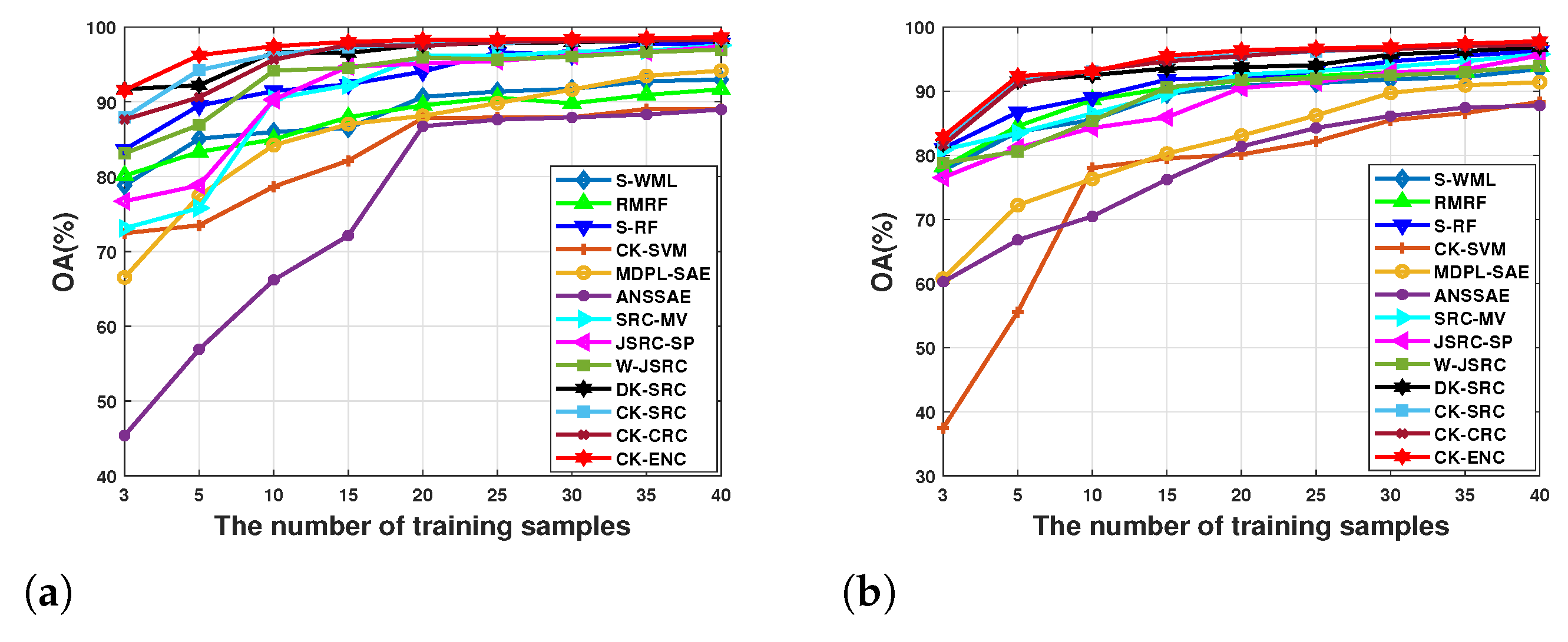
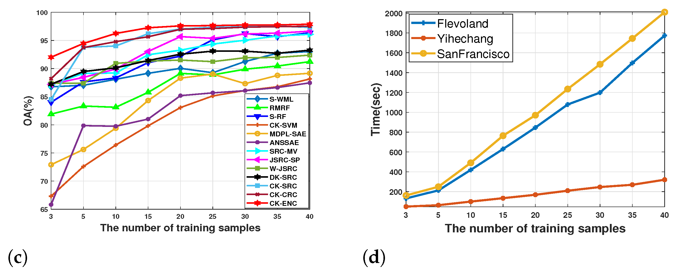
4.3. Effect of the Number of Training Samples

Figure 14a–c illustrates the effect of different numbers of training samples on the classification results, and the average OA value of 10 times random runs is reported. For all three datasets, the number of training samples per class varies from 3 to 40. Besides, we also report the execution time of the proposed CK-ENC under different numbers of training samples shown in Figure 14d. From Figure 14a–c, it can be seen that the OA values of all methods increase when the number of training samples increases. The proposed CK-ENC consistently yields higher OA values than other competitive methods. Furthermore, from Figure 14d, we could find that the execution time of CK-ENC increases as the number of training samples increases. Meanwhile, the OA value of CK-ENC is stable when the number of training samples is more than 20 per class. Based on the above discussion, for the compromise between time cost and classification accuracy, we have selected 20 training samples per class for all datasets in the above experiments.

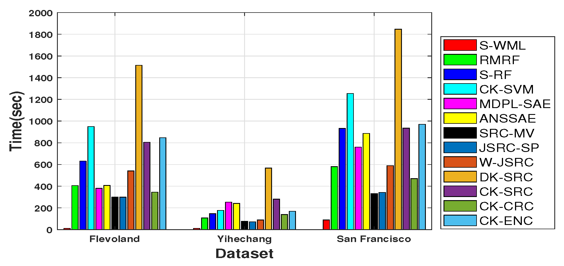
4.4. Efficiency Comparison

To assess the efficiency of the proposed CK-ENC, Figure 15 reports the execution time of different methods, including feature extraction time and classification time. For training-based methods, the execution time also includes model training time. Besides, these methods are all speed up by using the graphical processing unit (GPU). From Figure 15, we can see that S-WML has the shortest execution time because its classification framework is simple. As the GPU is used for acceleration, S-RF, MDPL-SAE, and ANSSAE methods have certain advantages in terms of execution time. However, compared with CK-ENC, the classification performance of these methods is undesirable. Restricted by the rectangular window operation, the execution time of DK-SRC is longer than other methods. In addition, benefiting from the role of superpixels, the proposed CK-ENC has a rather short time cost compared with DK-SRC. However, the execution time of the proposed CK-ENC is higher than SRC-MV, JSRC-SP, and W-JCRC. The main reason is that CK-ENC needs to calculate three different kernels, while SRC-MV, JSRC-SP, and W-JCRC only need to calculate one kernel. To sum up, taking both time consumption and accuracy into consideration, the proposed CK-ENC can get very competitive classification results.

5. Conclusions

This paper presents the CK-ENC method to achieve PolSAR image classification under the circumstance of limited training samples. Without any data projection, CK-ENC directly uses the PolSAR CV data as the benchmark data to avoid the loss of polarimetric information. Based on the superpixel segmentation of different scales, CK-ENC introduces a multi-feature extraction strategy to achieve better target contour preservation and enhance the robustness against speckles. In addition, a CK is constructed to effectively implement feature fusion, thereby improving the representation and discrimination capabilities of features. In this way, the proposed CK-ENC can achieve better classification performance. Moreover, to achieve more reliable results with limited training samples, we integrated the CK with the ENC for final PolSAR image classification. Experiments on three PolSAR datasets acquired from different systems evaluated the classification performance and effectiveness of the proposed CK-ENC. The classification results demonstrate that CK-ENC outperforms the state-of-the-art methods both in quantitative metrics and in visual quality, especially under the circumstance of limited training samples. In future work, we will generalize the CK-ENC method to classify dual-frequency PolSAR datasets.

References

- Lee, J.S.; Pottier, E. Polarimetric Radar Imaging: From Basic to Application; CRC Press: Boca Raton, FL, USA, 2017. [Google Scholar]
- Hänsch, R.; Hellwich, O. Skipping the real world: Classification of PolSAR images without explicit feature extraction. ISPRS J. Photogramm. Remote Sens. 2018, 140, 122–132. [Google Scholar] [CrossRef]
- Xiang, D.; Tao, T.; Ban, Y.; Yi, S. Man-made target detection from polarimetric SAR data via nonstationarity and asymmetry. IEEE J. Sel. Topics. Appl. Earth Observ. Remote Sens. 2016, 9, 1459–1469. [Google Scholar] [CrossRef]
- Akbari, V.; Anfinsen, S.N.; Doulgeris, A.P.; Eltoft, T.; Moser, G.; Serpico, S.B. Polarimetric SAR change detection with the complex Hotelling–Lawley trace statistic. IEEE Trans. Geosci. Remote Sens. 2016, 54, 3953–3966. [Google Scholar] [CrossRef] [Green Version]
- Biondi, F. Multi-chromatic analysis polarimetric interferometric synthetic aperture radar (MCAPolInSAR) for urban classification. Int. J. Remote Sens. 2019, 40, 3721–3750. [Google Scholar] [CrossRef]
- Lardeux, C.; Frison, P.L.; Tison, C.C.; Souyris, J.C.; Stoll, B.; Fruneau, B.; Rudant, J.P. Support vector machine for multifrequency SAR polarimetric data classification. IEEE Trans. Geosci. Remote Sens. 2009, 47, 4143–4152. [Google Scholar] [CrossRef]
- Song, W.; Li, M.; Zhang, P.; Wu, Y.; Tan, X.; An, L. Mixture WGΓ-MRF model for PolSAR image classification. IEEE Trans. Geosci. Remote Sens. 2018, 56, 905–920. [Google Scholar] [CrossRef]
- Du, P.J.; Samat, A.; Waske, B.; Liu, S.C.; Li, Z.H. Random forest and rotation forest for fully polarized SAR image classification using polarimetric and spatial features. ISPRS J. Photogramm. Remote Sens. 2015, 105, 38–53. [Google Scholar] [CrossRef]
- Zhou, Y.; Wang, H.; Xu, F.; Jin, Y.Q. Polarimetric SAR image classification using deep convolutional neural networks. IEEE Geosci. Remote Sens. Lett. 2016, 13, 1935–1939. [Google Scholar] [CrossRef]
- Chen, Y.; Jiao, L.; Li, Y.; Zhao, J. Multilayer projective dictionary pair learning and sparse autoencoder for PolSAR image classification. IEEE Trans. Geosci. Remote Sens. 2017, 55, 6683–6694. [Google Scholar] [CrossRef]
- Hu, Y.; Fan, J.; Wang, J. Classification of PolSAR images based on adaptive nonlocal stacked sparse autoencoder. IEEE Geosci. Remote Sens. Lett. 2018, 15, 1050–1054. [Google Scholar] [CrossRef]
- Wen, Z.; Wu, Q.; Liu, Z.; Pan, Q. Polar-spatial feature fusion learning with variational generative-discriminative network for PoLSAR classification. IEEE Trans. Geosci. Remote Sens. 2019, 57, 8914–8927. [Google Scholar] [CrossRef]
- Yamaguchi, Y.; Moriyama, T.; Ishido, M.; Yamada, H. Four component scattering model for polarimetric SAR image decomposition. IEEE Trans. Geosci. Remote Sens. 2005, 43, 1699–1706. [Google Scholar] [CrossRef]
- Arii, M.; van Zyl, J.J.; Kim, Y. Adaptive model-based decomposition of polarimetric SAR covariance matrices. IEEE Trans. Geosci. Remote Sens. 2011, 49, 1104–1113. [Google Scholar] [CrossRef]
- An, W.; Cui, Y.; Yang, J. Three-component model-based decomposition for polarimetric SAR data. IEEE Trans. Geosci. Remote Sens. 2010, 48, 2732–2739. [Google Scholar]
- Lee, J.S.; Grunes, M.R.; Pottier, E.; Ferro-Famil, L. Unsupervised terrain classification preserving polarimetric scattering characteristics. IEEE Trans. Geosci. Remote Sens. 2004, 42, 722–731. [Google Scholar]
- Clound, S.R.; Pottier, E. An entropy based classification scheme for land applications of polarimetric SAR. IEEE Trans. Geosci. Remote Sens. 1997, 35, 68–78. [Google Scholar]
- Clound, S.R.; Pottier, E. Integrating color features in polarimetric SAR image classification. IEEE Trans. Geosci. Remote Sens. 2014, 52, 2197–2216. [Google Scholar]
- He, C.; Li, S.; Liao, Z.; Liao, M. Texture Classification of PolSAR Data Based on Sparse Coding of Wavelet Polarization Textons. IEEE Trans. Geosci. Remote Sens. 2013, 51, 4576–4590. [Google Scholar] [CrossRef]
- Kim, H.; Hirose, A. Polarization feature extraction using quaternion neural networks for flexible unsupervised PolSAR land classification. In Proceedings of the IEEE International Geoscience and Remote Sensing Symposium (IGARSS), Valencia, Spain, 22–27 July 2018; pp. 2378–2381. [Google Scholar]
- Dong, H.; Xu, X.; Sui, H.; Xu, F.; Liu, J. Copula-based joint statistical model for polarimetric features and its application in PolSAR image classification. IEEE Trans. Geosci. Remote Sens. 2017, 55, 5777–5789. [Google Scholar] [CrossRef]
- He, C.; He, B.; Tu, M.; Wang, Y.; Qu, T.; Wang, D.; Liao, M. Fully Convolutional Networks and a Manifold Graph Embedding-Based Algorithm for PolSAR Image Classification. Remote Sens. 2020, 12, 1467. [Google Scholar] [CrossRef]
- Lee, J.S.; Grunes, M.R.; Kwok, R. Classification of multi-look polarimetric SAR imagery based on the complex Wishart distribution. Int. J. Remote Sens. 1994, 15, 2299–2311. [Google Scholar] [CrossRef]
- Lee, J.S.; Schuler, D.L.; Lang, R.H.; Ranson, K.J. K-Distribution for Multi-Look Processed Polarimetric SAR Imagery. In Proceedings of the IEEE International Geoscience and Remote Sensing Symposium, Pasadena, PA, USA, 8–12 August 1994; pp. 2179–2181. [Google Scholar]
- Freitas, C.C.; Frery, A.C.; Correia, A.H. The polarimetric G distribution for SAR data analysis. Environmetrics 2005, 16, 13–31. [Google Scholar] [CrossRef]
- Chi, L.; Liao, W.; Li, H.C.; Fu, K.; Philips, W. Unsupervised classification of multilook polarimetric SAR data using spatially variant wishart mixture model with double constraints. IEEE Trans. Geosci. Remote Sens. 2018, 56, 5600–5613. [Google Scholar]
- Yang, F.; Gao, W.; Xu, B.; Yang, J. Multi-frequency polarimetric SAR classification based on Riemannian manifold and simultaneous sparse representation. Remote Sens. 2015, 7, 8469–8488. [Google Scholar] [CrossRef] [Green Version]
- Yang, X.; Yang, W.; Song, H.; Huang, P. Polarimetric SAR image classification using geodesic distances and composite kernels. IEEE J. Sel. Topics. Appl. Earth Observ. Remote Sens. 2018, 11, 1606–1614. [Google Scholar] [CrossRef]
- Hänsch, R. Complex-Valued Multi-Layer Perceptrons—An Application to Polarimetric SAR Data. Photogramm. Eng. Remote Sens. 2010, 76, 1081–1088. [Google Scholar] [CrossRef]
- Kinugawa, K.; Shang, F.; Usami, N.; Hirose, A. Isotropization of Quaternion-Neural-Network-Based PolSAR Adaptive Land Classification in Poincare-Sphere Parameter Space. IEEE Geosci. Remote Sens. Lett. 2018, 15, 1234–1238. [Google Scholar] [CrossRef]
- Shang, F.; Hirose, A. Quaternion neural-network-based PolSAR land classification in Poincare- sphereparameter space. IEEE Trans. Geosci. Remote Sens. 2014, 52, 5693–5703. [Google Scholar] [CrossRef]
- Zhang, Z.; Wang, H.; Xu, F.; Jin, Y.Q. Complex-valued convolutional neural network and its application in polarimetric sar image classification. IEEE Trans. Geosci. Remote Sens. 2017, 55, 7177–7188. [Google Scholar] [CrossRef]
- Cao, Y.; Wu, Y.; Zhang, P.; Liang, W.; Li, M. Pixel-wise PolSAR image classification via a novel complex-valued deep fully convolutional network. Remote Sens. 2019, 11, 2653. [Google Scholar] [CrossRef] [Green Version]
- Tan, X.; Li, M.; Zhang, P.; Wu, Y.; Song, W. Complex-valued 3-D convolutional neural network for PolSAR image classification. IEEE Geosci. Remote Sens. Lett. 2019, in press. [Google Scholar] [CrossRef]
- Liu, W.; Yang, J.; Li, P.; Han, Y.; Zhao, J.; Shi, H. A novel object-based supervised classification method with active learning and random forest for PolSAR imagery. Remote Sens. 2018, 10, 1092. [Google Scholar] [CrossRef] [Green Version]
- Zhong, N.; Yang, W.; Cherian, A.; Yang, X.; Xia, G.; Liao, M. Unsupervised classification of polarimetric SAR images via Riemannian sparse coding. IEEE Trans. Geosci. Remote Sens. 2017, 55, 5381–5390. [Google Scholar] [CrossRef]
- Liu, B.; Hu, H.; Wang, H.; Wang, K.; Liu, X.; Yu, X. Superpixel-based classification with an adaptive number of classes for polarimetric SAR images. IEEE Trans. Geosci. Remote Sens. 2013, 51, 907–924. [Google Scholar] [CrossRef]
- Qin, F.; Guo, J.; Lang, F. Superpixel segmentation for polarimetric SAR imagery using local iterative clustering. IEEE Geosci. Remote Sens. Lett. 2015, 12, 13–17. [Google Scholar]
- Wu, Y.; Ji, K.; Yu, W.; Su, Y. Region-based classification of polarimetric SAR images using Wishart MRF. IEEE Geosci. Remote Sens. Lett. 2008, 5, 668–672. [Google Scholar] [CrossRef]
- Yang, R.; Hu, Z.; Liu, Y.; Xu, Z. A Novel Polarimetric SAR Classification Method Integrating Pixel-Based and Patch-Based Classification. IEEE Geosci. Remote Sens. Lett. 2019, 17, 431–435. [Google Scholar] [CrossRef]
- Deledalle, C.A.; Denis, L.; Tupin, F.; Reigber, A.; Jäger, M. NL-SAR: A unified nonlocal framework for resolution-preserving (Pol)(In)SAR denoising. IEEE Trans. Geosci. Remote Sens. 2015, 53, 2021–2038. [Google Scholar] [CrossRef] [Green Version]
- Wang, J.; Jiao, L.; Wang, S.; Hou, B.; Liu, F. Adaptive nonlocal spatial–spectral kernel for hyperspectral imagery classification. IEEE J. Sel. Topics. Appl. Earth Observ. Remote Sens. 2016, 9, 4086–4101. [Google Scholar] [CrossRef]
- Jia, L.; Li, M.; Wu, Y.; Zhang, P.; Liu, G.; Chen, H.; An, L. SAR image change detection based on iterative label information composite kernel supervised by anisotropic texture. IEEE Trans. Geosci. Remote Sens. 2015, 53, 3960–3973. [Google Scholar] [CrossRef]
- Tuia, D.; Ratle, F.; Pozdnoukhov, A.; Camps-Valls, G. Multisource composite kernels for urban-image classification. IEEE Geosci. Remote Sens. Lett. 2010, 7, 88–92. [Google Scholar] [CrossRef] [Green Version]
- Zou, H.; Hastie, T. Regularization and variable selection via the elastic net. J. R. Stat. Soc. B 2005, 67, 301–320. [Google Scholar] [CrossRef] [Green Version]
- Li, W.; Du, Q.; Zhang, F.; Hu, W. Hyperspectral image classification by fusing collaborative and sparse representations. IEEE J. Sel. Topics. Appl. Earth Observ. Remote Sens. 2016, 9, 4178–4187. [Google Scholar] [CrossRef]
- Cao, F.; Hong, W.; Wu, Y.; Pottier, E. An unsupervised segmentation with an adaptive number of clusters using the SPAN/H/α/A space and the complex Wishart clustering for fully polarimetric SAR data analysis. IEEE Trans. Geosci. Remote Sens. 2007, 45, 3454–3467. [Google Scholar] [CrossRef]
- Arsigny, V.; Fillard, P.; Pennec, X.; Ayache, N. Log-euclidean metrics for fast and simple calculus on diffusion tensors. Mag. Resonance Med. 2006, 56, 411–4216. [Google Scholar] [CrossRef]
- Sra, S. Positive definite matrices and the S-divergence. Proc. Amer. Math. Soc. 2016, 144, 2787–2797. [Google Scholar] [CrossRef] [Green Version]
- Mairal, J.; Bach, F.; Ponce, J.; Sapiro, G. Online learning for matrix factorization and sparse coding. J. Mach. Learn. Res. 2010, 11, 19–60. [Google Scholar]
- Feng, J.; Cao, Z.; Pi, Y. Polarimetric contextual classification of PolSAR images using sparse representation and superpixels. Remote Sens. 2014, 6, 7158–7181. [Google Scholar] [CrossRef] [Green Version]
- Geng, J.; Wang, H.; Fan, J.; Ma, X.; Wang, B. Wishart distance-based joint collaborative representation for polarimetric SAR image classification. IET Radar Sonar Navigat. 2017, 11, 1620–1628. [Google Scholar] [CrossRef]
- Chang, C.C.; Lin, C.J. LIBSVM: A library for Support Vector Machines. ACM Trans. Intell. Syst. Technol. 2011, 2. [Google Scholar] [CrossRef]
Figure 1.
Framework of the proposed CK-ENC.
Figure 2.
Scheme of the nonlocal Wishart weighted feature (NWWF) extraction.
Figure 3.
The Flevoland dataset. (a) Pauli RGB image; (b) ground truth; (c) color code of the different classes.
Figure 4.
The Yihechang dataset. (a) Pauli RGB image; (b) ground truth; (c) color code of the different classes.
Figure 5.
The San Francisco dataset. (a) Pauli RGB image; (b) ground truth; (c) color code of the different classes.
Figure 6.
Impact of the superpixel size R for (a) Flevoland dataset, (b) Yihechang dataset, and (c) San Francisco dataset.
Figure 7.
Impact of the regularization parameters for (a) Flevoland dataset, (b) Yihechang dataset, and (c) San Francisco dataset.
Figure 8.
Classification results of the Flevoland dataset with different methods.
Figure 9.
Classification results of the Yihechang dataset with different methods.
Figure 10.
Classification results of the San Franciso dataset with different methods.
Figure 11.
Impact of the kernel parameter for three PolSAR datasets.
Figure 12.
Effect of the kernel weight parameters for (a) Flevoland dataset, (b) Yihechang dataset, and (c) San Francisco dataset.
Figure 13.
Classification results on the San Francisco dataset (a) without the polarimetirc second-order matrix kernel, and (b) with the polarimetirc second-order matrix kernel.
Figure 14.
Effect of the number of training samples for (a) Flevoland dataset, (b) Yihechang dataset, and (c) San Francisco dataset. (d) Execution time (in seconds) of CK-ENC under different numbers of training samples for the three PolSAR datasets.
Figure 15.
Execution time (in seconds) in the three PolSAR datasets.