Article

Assessing the Performance of ICESat-2/ATLAS Multi-Channel Photon Data for Estimating Ground Topography in Forested Terrain

1
Centre for Forest Operations and Environment, Northeast Forestry University, Harbin 150040, China
2
Institute of Theoretical Physics, Federal Institute of Technology (ETH), 8092 Zurich, Switzerland
*
Author to whom correspondence should be addressed.
Remote Sens. 2020, 12(13), 2084; https://0-doi-org.brum.beds.ac.uk/10.3390/rs12132084
Submission received: 26 May 2020 / Revised: 26 June 2020 / Accepted: 26 June 2020 / Published: 29 June 2020

Abstract

:
As a continuation of Ice, Cloud, and Land Elevation Satellite-1 (ICESat-1), the ICESat-2/Advanced Topographic Laser Altimeter System (ATLAS) employs a micro-pulse multi-beam photon counting approach to produce photon data for measuring global terrain. Few studies have assessed the accuracy of different ATLAS channels in retrieving ground topography in forested terrain. This study aims to assess the accuracy of measuring ground topography in forested terrain using different ATLAS channels and the correlation between laser intensity parameters, laser pointing angle parameters, and elevation error. The accuracy of ground topography measured by the ATLAS footprints is evaluated by comparing the derived Digital Terrain Model (DTM) from the ATL03 (Global Geolocated Photon Data) and ATL08 (Land and Vegetation Height) products with that from the airborne Light Detection And Ranging (LiDAR). Results show that the ATLAS product performed well in the study area at all laser intensities and laser pointing angles, and correlations were found between the ATLAS DTM and airborne LiDAR DTM (coefficient of determination––R2 = 1.00, root mean squared error––RMSE = 0.75 m). Considering different laser intensities, there is a significant correlation between the tx_pulse_energy parameter and elevation error. With different laser pointing angles, there is no significant correlation between the tx_pulse_skew_est, tx_pulse_width_lower, tx_pulse_width_upper parameters and the elevation error.

1. Introduction

The spatial structure of forested terrain is listed as an important indicator for monitoring carbon stocks by the International Union of Forest Research Organizations (IUFRO) [1,2]. Assessing ground topography in forested terrain is a prerequisite to accurately determine the forest spatial structure; therefore, high spatial resolution modeling is necessary to characterize forest ecosystems [3,4]. Most optical remote sensing systems can measure ground topography in forested terrain; however, they have poor measurement accuracy (elevation difference = 2.9 m to 4.9 m) [5,6]. Spaceborne [7], airborne [8,9], and terrestrial [10,11] Light Detection And Ranging (LiDAR) systems have shown great potential for acquiring accurate topographic information in this field. Although airborne and terrestrial LiDAR can accurately quantify ground topography in forested terrain, these methods remain largely impractical at large spatial scales due to high data acquisition costs [8,12,13,14]. Spaceborne LiDAR is unique since it comes with low acquisition costs and provides a synoptic perspective of certain plot-level details from orbit [15].
The Ice, Cloud, and land Elevation satellite-1 (ICESat-1) [16], the Global Ecosystem Dynamics Investigation (GEDI) [17], and the Ice, Cloud, and land Elevation satellite-2 (ICESat-2) [18] are typical spaceborne LiDAR systems. ICESat-1 and GEDI carry large-footprint and waveform LiDAR systems. The Geoscience Laser Altimeter System (GLAS) instrument aboard ICESat-1 was launched in 2003 and decommissioned in 2009 [19]. GLAS is the first spaceborne LiDAR instrument designed to make global observations. GLAS operates a single laser beam from a ~600 km orbit at 40 Hz and has a 70 m diameter footprint and a ~170 m sampling rate along track.
GLAS waveform data has been successfully used to estimate the vertical structure of forest terrain, including ground topography and canopy heights [19,20,21]. Harding et al. [20] found that the waveform was an accurate representation of the canopy height distribution within a GLAS footprint. Lefsky et al. [21] observed that the models combing GLAS waveforms and Shuttle Radar Topography Mission (SRTM) could explain ~59%–68% of the variance in the field-measured forest canopy height (root mean squared error––RMSE = 4.85–12.66 m); however, sloped ground in forested terrain reduced the canopy height accuracy by using waveform data. Chen [22] found that the ground topography in forested terrain was the critical factor affecting the accurate measurement of canopy height using waveform data, and with increasing forest terrain complexity, the accuracy of estimating forest canopy height decreased. Fang et al. [23] found that in forested terrain with complex ground topography, the GLAS waveform was characterized by multiple energy peaks, in which the ground topography might be broadened and mixed, making the extraction of canopy height difficult. In order to quantify the influence of ground topography on canopy height estimation using GLAS waveform data, Lee et al. [24] found that without slope correction, the canopy height could be overestimated by 3 m over a 15 degree slope. Removing the ground topography in forested terrain from large LiDAR footprint could improve the accuracy of canopy height estimates. Claudia et al. [25] revealed that GLAS height estimates were accurate for areas with a slope up to 10 degrees, whereas the waveform results for areas above 15 degrees were problematic. Ten-to-fifteen degree slopes have been found to be a critical crossover point. The aforementioned studies demonstrated that it was feasible to extract ground topography in forested terrain and canopy height from spaceborne waveform data at stand level; however, the accuracy of canopy height estimation was largely determined by the ground topography, and extracting canopy height across a large LiDAR footprint using waveform data over hilly or mountainous regions is a great challenge. The GEDI was launched on 5 December 2018; however, the GEDI spaceborne data has just recently been released, and no related study was found [26].
The Advanced Topographic Laser Altimeter System (ATLAS) instrument aboard ICESat-2 was launched on 15 September 2018, and data was released on 30 May 2019. ATLAS is the first spaceborne photon-counting LiDAR instrument designed for continuous global observation of Earth [27,28,29]. Different from the GLAS waveform-digitizing LiDAR system, ATLAS only responds to the presence of return signals and records the time tags with an output of 0 or 1; however, it does not record the return waveform [30,31,32]. ATLAS operates six laser beams from a ~600 km orbit at 10 kHz and has a footprint (17 m in diameter) sampling rate of ~0.7 m along-track [33,34]. The center-to-center spacing along a track for ATLAS is narrower than that of GLAS (170 m). The high repetition rate enables ATLAS to obtain nearly continuous tracking information, which is necessary to measure the ground topography in forested terrain. While the GLAS LiDAR system uses a laser beam, the ATLAS configuration uses a diffractive optical element to split the laser into six beams arranged as three beam pairs, each of which consists of a strong and weak energy beam at a 4:1 ratio, allowing for local slope determination between each beam pair as well as compensation for varying surface reflectance [27,33,34]. The travel time of each detected photon is used to determine a unique XYZ location on the Earth’s surface [35,36]. After ATLAS data was released, Neuenschwander found good correlations between matching Digital Terrain Model (DTM) from airborne LiDAR data and ATLAS data (R2 = 0.99, RMSE = 0.85 m) [37]. Wang et al. found that the overall mean difference and RMSE values between the ground elevations retrieved from the ICESat-2 data and the airborne LiDAR-derived ground elevations are −0.61 m and 1.96 m, respectively [38]. However, he primarily examined the retrieved canopy height accuracy from the ICESat-2 strong beam and did not analyze the accuracy of the ICESat-2 weak beam. Under the same orbital conditions, ATLAS can acquire more continuous photon cloud data using the six-beam instrument with different laser pointing angles and laser intensities. The measurement accuracy of the different ATLAS channels remains to be quantified [39]. To the authors’ knowledge, only a few studies have been carried out to analyze the multi-beam geometrical features for measuring ground topography in forested terrain from photon-counting data onboard ICESat-2. Therefore, the effective quantifying of the ground topography in forested terrain using the six-beam photon-counting data is essential to quantify the performance of the unique photon-counting instrument onboard ICESat-2.
The objective of this study is to assess the performance of the ICESat-2/ATLAS multi-channel photon data for estimating ground topography in forested terrain by comparing the derived ground topography from different ATLAS beam photon-counting data with that from Goddard’s LiDAR, Hyperspectral and Thermal imager (G-LiHT) data. The paper also analyzes the correlation between laser intensity parameters, laser pointing angle parameters, and estimated ground topography error in forested terrain.

2. Materials and Methods

2.1. Study Area

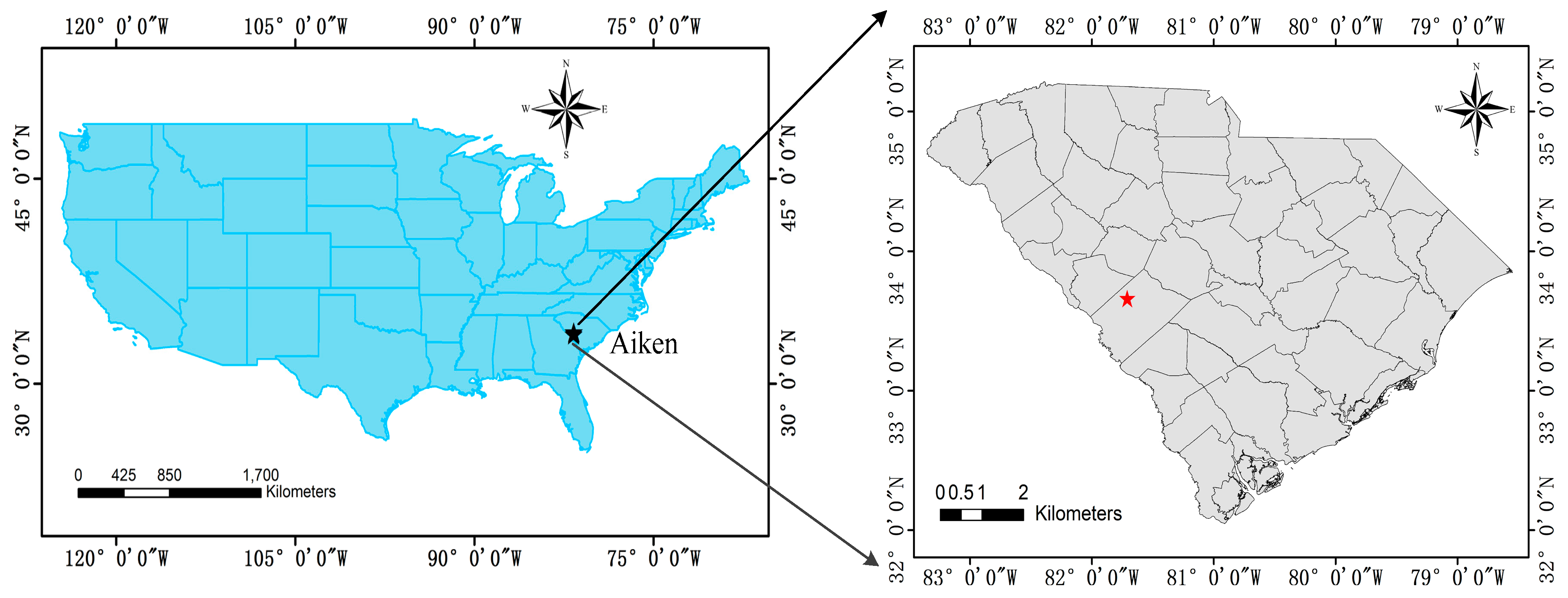
The study area (33.564°N, 81°684′W) is a forested area within the City of Aiken, South Carolina, USA (Figure 1). Vegetation footprint types in the study area include cultivated land (0.04%), forest (88.52%), shrubland (0.51%), wetland (6.97%), and artificial surfaces (3.95%) [39]. The upland forest has many tree species, including sand post oak (Quercus margaretta), loblolly pine, water oak (Quercus nigra), hickory (Carya), and turkey oak (Quercus laevis) [40]. The elevation of the study area ranges from 91 m to 164 m. Vegetation coverage in the study area ranges from 25% to 66%.

2.2. Data

The ICESat-2 mission produces along-track ground topography in forested terrain that includes telemetry data (ATL00), reformatted telemetry (ATL01), science unit converted telemetry (ATL02), global geolocated photon data (ATL03), land vegetation elevation (ATL08), and a land/canopy grid (ATL18) [37,38,39,40,41]. ATL00, ATL01, and ATL02 are original photon data sets without scientific algorithms. ATL03 is the geolocated photon cloud and serves as the input data for each of the higher-level data products such as ATL08 and ATL18. The ATL08 algorithm was developed specifically for the extraction of terrain and canopy heights from the ATL03 photon cloud data, and the ATL08 geophysical data product has a 100 m step size in the along-track direction [33]. The ATL03 product not only includes latitude, longitude, height, and signal photon confidence level of each received photon, but also includes tx_pulse_energy, tx_pulse_skew_est, tx_pulse_width_lower, and tx_pulse_width_upper parameters, which may be related to laser intensity and laser pointing angle [37]. All ICESat-2 data products were acquired from https://search.earthdata.nasa.gov.
Here the ATL03 product parameters were used, including lat_ph, lon_ph, h_ph, geoid, delta_time, signal_conf_ph, sc_orient, tx_pulse_energy, tx_pulse_skew_est, tx_pulse_width_lower, and tx_pulse_width_upper. The names and corresponding descriptions of product parameters are listed in Table 1 [37,38,39]. In order to reduce the influence of noise photons in forested terrain ground topography measurement, a signal_conf_ph of 4 was used as the signal photon parameter evaluation standard.
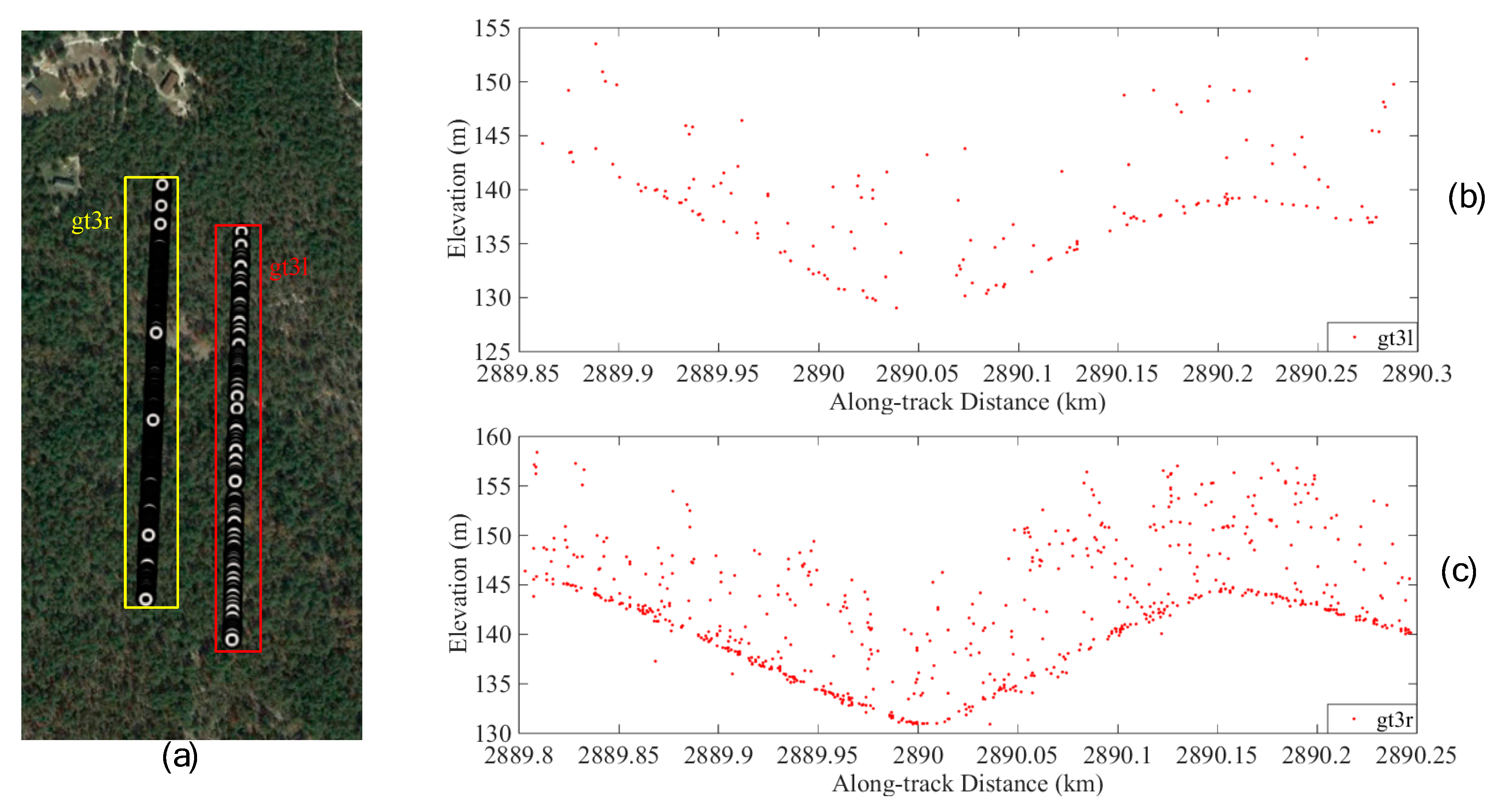
A diagram of ICESat-2 for estimating ground topography in forested terrain is illustrated in Figure 2. The forward orientation (sc_orient=1) corresponds to ATLAS traveling along the +x direction in the ATLAS instrument reference frame [41,42,43]. The ATLAS signal photon shown in the yellow square represents the photons detected from the gt3r laser channel. The ATLAS footprint shown in the red square represents the photons detected from the gt3l laser channel. The number of photons in the gt3l channel is less than in the gt3r channel, which is due to the backward orientation of ATLAS [43]. The photon level in the along-track direction was selected to calculate the ground topography in forested terrain. In the right figures, the two laser beams are 90 m apart. The ground topography measured by the two laser beams is similar, and the terrain elevation ranges from 130 m–145 m.
Due to the influence of sunlight as well as atmospheric and system noise, a large number of noise photons are present in the ATLAS data, which seriously reduce the ground elevation measurement accuracy. In order to improve the estimation accuracy of ATLAS photon data, NASA proposed a Differential, Regressive, and Gaussian Adaptive Nearest Neighbor (DRAGANN) method and ATL08 data classified algorithm to filter out noise photon data and classify ground photons [41,42,43]. In order to explore the estimation accuracy of forested terrain from ATLAS data, this contribution chose to associate the ATL08 classified label with the ATL03 photon data and used the ground signal photons flag mentioned in ATL08 as ground photons to establish an ATLAS-based DTM (Table 2) [37].
To assess the accuracy of the six beam-ATLAS DTM, the DTM obtained from the ATLAS data was compared with airborne discrete-return LiDAR data, collected for the same longitude and latitude using the multi-sensor instrument G-LiHT [44]. G-LiHT provides distributed laser pulses for measuring ground topography and canopy heights (Table 3) [45].
Both Level 2 and Level 3 products along the flight transects were generated from airborne LiDAR data from the G-LiHT science team. The DTM has a 1 m-resolution and was released as a Tag Image File Format (TIFF) profile. The DTM was assessed to validate the ground topography accuracy [44,
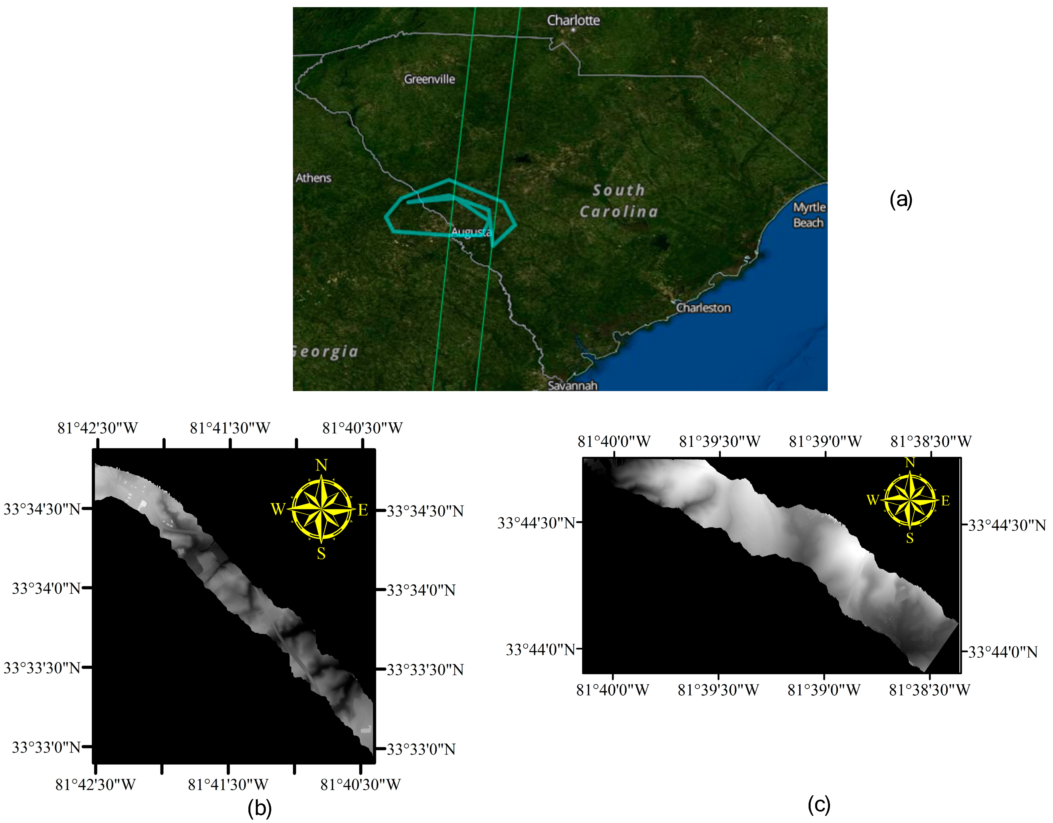
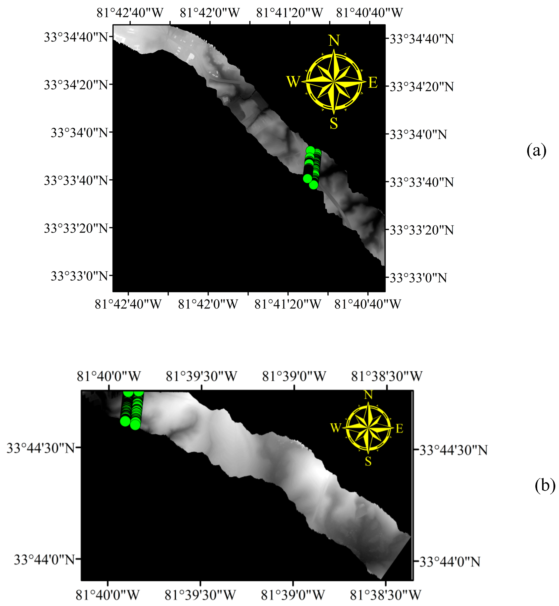
45]. The trajectory of the G-LiHT KML (Keyhole Markup Language) data (blue line) and ATLAS data (green line) illustrates the location of the study area of the NASA EARTHDATA (Figure 3). This illustration also includes two G-LiHT DTM profiles used in the study, AMIGACarb_Augusta_FIA_Sep2011_l16s597_DTM.tif and AMIGACarb_Augusta_FIA_ Sep2011_ l40s557_DTM.tif, respectively.

2.3. Methodology

The primary challenge of this contribution centers on reducing the influence of noise photons on the ground elevation data derived from ICESat-2 data, distinguishing canopy signal photons and ground signal photons, and matching the ATL03, ATL08, and G-LIHT data. Although ATLAS data has more noise photons, the NASA official team used the DRAGANN and an algorithm for determining Land Vegetation along-track to provide classification labels (classed_pc_flag) for the photon data [43]. In this contribution, the ground signal photon classification label ATL08 is used for ground photons, and the DTMATLAS will be established based on ATL03 data and ATL08 label. This contribution presents a quantitative assessment of the ground topography in forested terrain using ATL03 and ATL08 data compared to airborne G-LiHT LiDAR data.
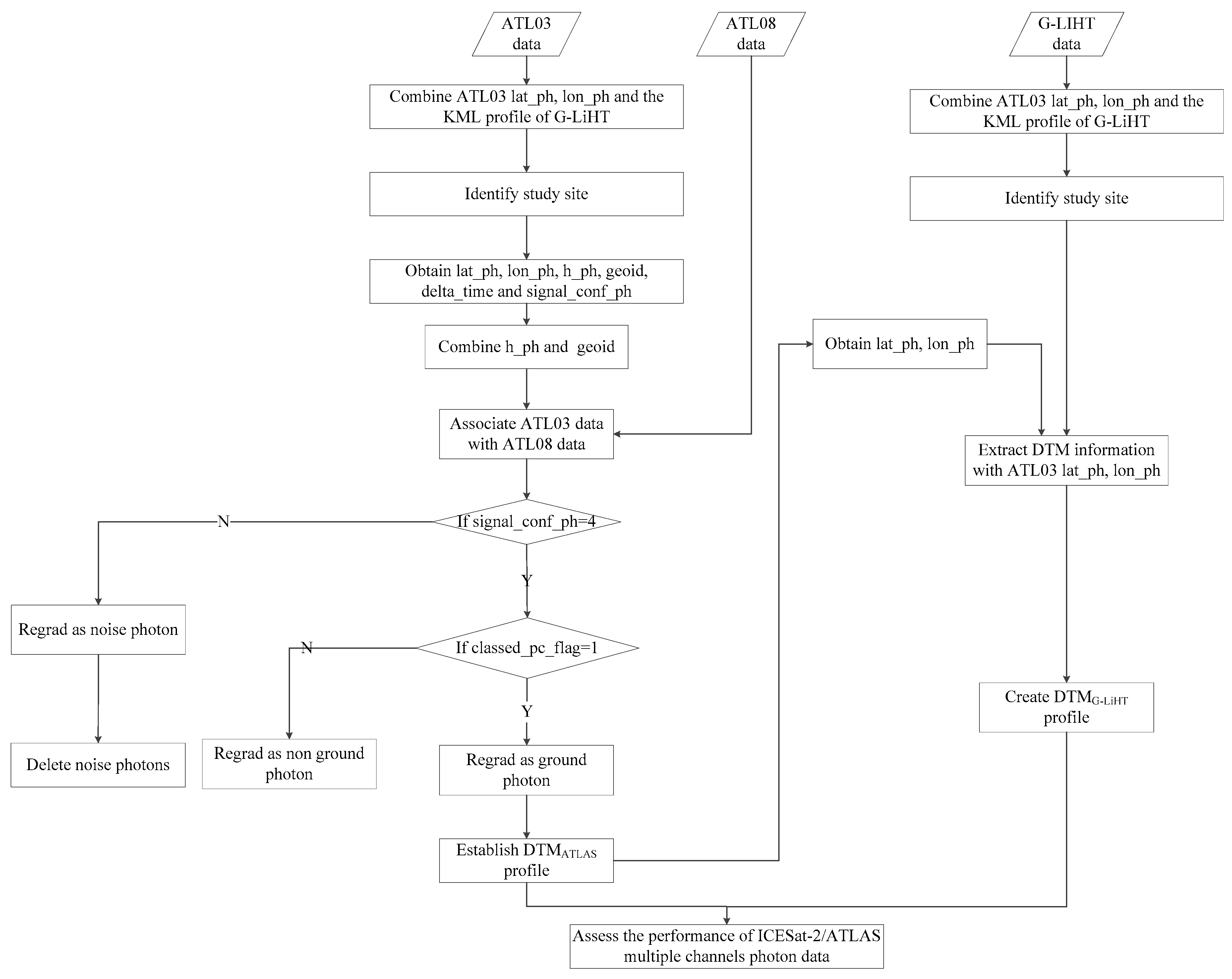
The geolocation between the ATLAS and G-LiHT data is not completely along orbit; therefore, this paper proposes an approach based on the ATL03 profile to match these two datasets (Figure 3). To clearly illustrate the proposed methodology, an overview of the major steps is exhibited in Figure 4 and described as follows:
(1) Identifying study site. In this step, we combine ATL03 lat_ph, lon_ph, and G-LiHT KML profile and identify the study site.
(2) Obtain parameters from the ATL03 and ATL08 data by matching different channels under the same orbit conditions using time tags (delta_time in ATL03 HDF5 profile). To extract the photon’s height (h_ph which is relative to the WGS-84 ellipsoid), latitude (lat_ph) and longitude (lon_ph), signal_conf_ph, sc_orient, tx_pulse_energy, tx_pulse_skew_est, tx_pulse_width_lower, and tx_pulse_width_upper parameters from the ATL03 HDF5 profile, combine the geoid and h_ph by interpolating. Extract the photon classification parameters (classed_pc_flag), classed_pc_indx, and ph_segment_id parameters from the ATL08 HDF5 profile.
(3) Establishing the relationship between ATL03 and ATL08 data photon classification parameters by classed_pc_indx, ph_segment_id and applying each photon classification label from ATL08 to each photon data from ATL03.
(4) Establishing the DTMATLAS. The photons with a signal confidence flag from high confidence (signal_confidence = 4 in ATL03 HDF5 profile) and photon classification parameter (classed_pc_flag=1 in ATL08 HDF5 profile) were used to establish the DTMATL03.
(5) Obtaining the DTMG-LiHT. In this step, we extract the latitude-longitude information from DTMATL03 to match the DTMG-LiHT profile corresponding position generated from G-LiHT and generated DTMG-LiHT with the corresponding ATLAS footprint latitude-longitude. If the absolute difference between the elevation of ATLAS ground photons and the corresponding elevation of the DTMG-LiHT is more than 20 m, this photon was classified as an invalid ground photon.
(6) Assessing the performance of ICESat-2/ATLAS multiple channels photon data. In this final step, we compare the DTMATL03 profile with the corresponding DTMG-LiHT profile, compute and analyze the evaluating indicator from different channels. In order to quantify the influence of different laser intensity parameters and laser pointing angle parameters on the estimation accuracy of ground elevation, corresponding four parameters as follow: tx_pulse_energy, tx_pulse_skew_est, tx_pulse_width_lower and tx_pulse_width_upper are extracted and analyzed the relationship between the four parameters and elevation errors.
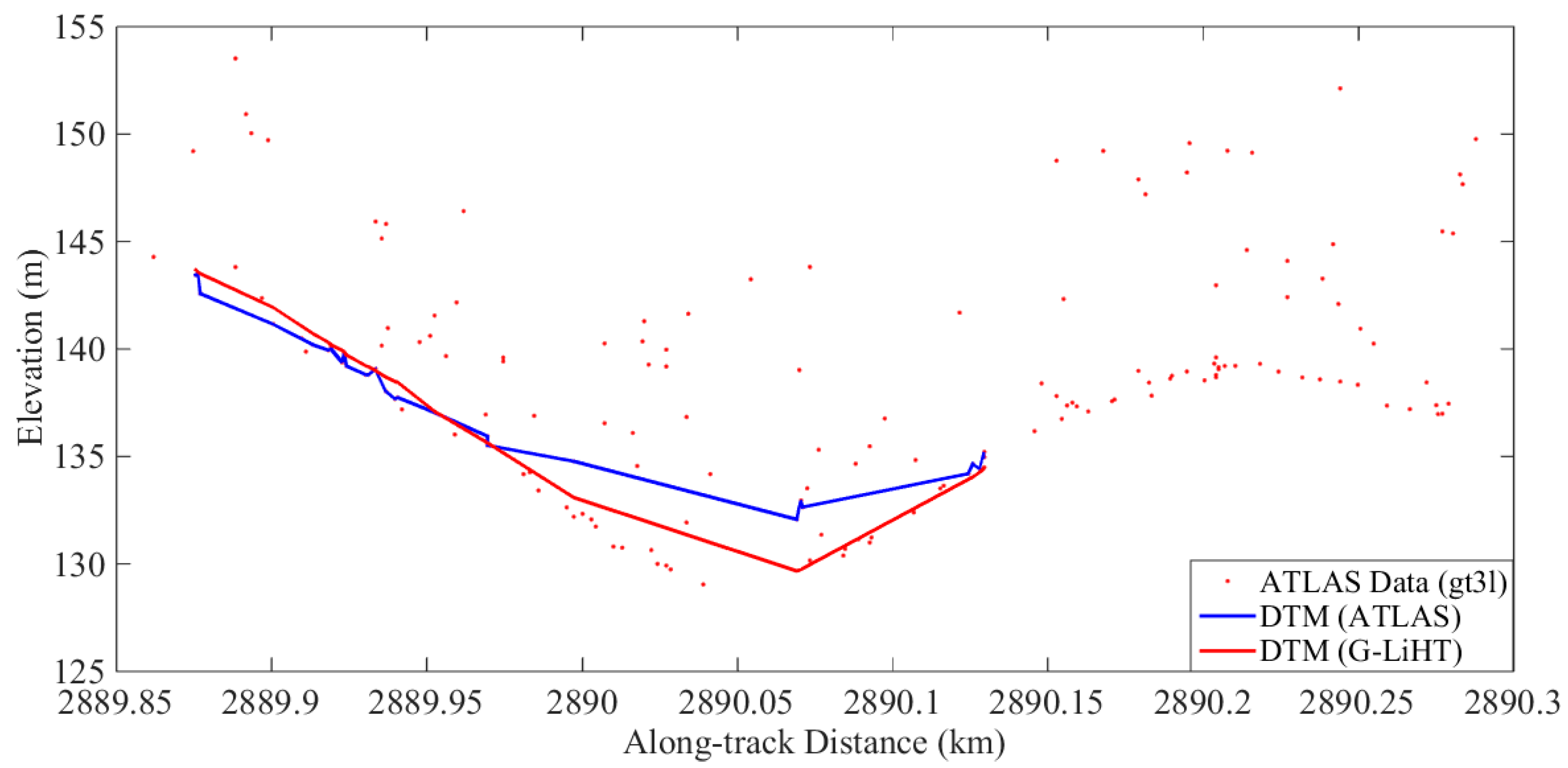
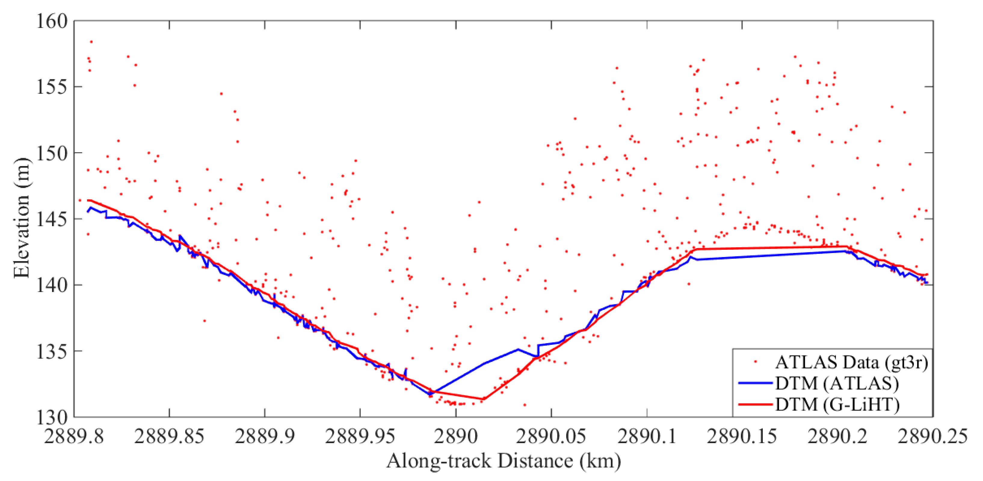
The Figure 5 shows the DTM files of G-LiHT and ATLAS photon data corresponding to the two tracks in the study area. The green dots are ATLAS footprints.

2.4. Accuracy Evaluation

DTM data derived from airborne G-LiHT LiDAR data were utilized to assess the accuracy of the ATLAS-derived ground elevations. The ground elevation errors in the ATLAS data mentioned in this contribution are calculated by subtracting the G-LiHT elevations from the ATLAS elevations [38]. Seven statistical variables, including root mean squared error (RMSE), mean absolute error (MAE), coefficient of determination (R2), mean error (ME), Pearson correlation coefficient, Spearman correlation coefficient, and Kendall correlation coefficient between the ground elevations and the corresponding G-LiHT’s DTM values were calculated to quantitatively evaluate the accuracy of the ATLAS-derived ground elevations. Three statistical variables, Pearson correlation coefficient, Spearman correlation coefficient, and Kendall correlation coefficient between the elevation errors and the corresponding laser intensity parameter and laser pointing angle parameters were calculated to quantitatively evaluate the correlation of laser intensities and laser pointing angles with the elevation error in estimating ground topography in forested terrain.

3. Results

Result Comparisons

The G-LiHT data in the study was acquired in 2011 and are not temporally coincident with ICESat-2/ATLAS. However, the availability of aerial-based LiDAR data for the study area makes it feasible to validate the ground topography from ATL03. The ATL03 gt3l channel photon data and gt3r channel photon data over the study are plotted with the G-LiHT data shown in Figure 6 and Figure 7, respectively. The scatterplots of the ATL03 (gt3l and gt3r) ground elevations versus the G-LiHT ground elevations are shown in Figure 8 and Figure 9. The statistical indicators, namely the RMSE, MAE, R2, ME, Pearson correlation coefficient, Spearman correlation coefficient, and Kendall correlation coefficient are listed in Table 4.
Figure 6 and Figure 7 show the comparisons of elevations from the ATLAS DTM and G-LiHT DTM for multiple channels, and both are referenced to the WGS84 geoid. The ATLAS DTM (blue line) and G-LiHT’s DTM (red line) had a similar performance (Figure 6 and Figure 7). The ATLAS gt3l channel (weak beam) photon cloud contains fewer signal photons than the gt3r channel (strong beam). The photons near the blue line and red line denote the ground topography photons. A t-test showed that no significant difference exists between these two regression lines in Figure 8 and Figure 9 at a 95% confidence level. The ATLAS gt3r channel (Figure 7 and Figure 9) signal photons show a clearer depiction of the ground topography than the ATLAS gt3l channel (Figure 6 and Figure 8).
The R2 of the all experiments are higher than 0.99 (Table 4). The mean ME and RMSE values of all ground photons are 0.3 m and 0.75 m, respectively. For gt1l, gt1r, gt2l, gt2r, gt3l, and gt3r, the ME values are −0.05 m, 0.27 m, 0.59 m, 0.04 m, 0.45 m, and 0.49 m, and the RMSE values are 0.69 m, 0.55 m, 0.80 m, 1.03 m, 0.78 m, and 0.64 m, respectively. In general, the statistical indicators for pointing right (namely strong beam) perform better than those for pointing left (namely weak beam) for all data sets. A possible reason is that the signal photon density from the strong beam channels is significantly higher than that of the weak beam channels.
All laser intensities and laser pointing angles from the ATL03 product performed well in the study site (Table 4, Figure 8 and Figure 9). The ATL03 data have good ground elevation estimation accuracy, and the ATL08 algorithm can effectively filter out noise photon and classify ground photons in the forested terrain ground topography estimation process.

4. Discussion

In order to study the influence of laser intensity and laser pointing angle on ground elevation estimation accuracy, the ATLAS data errors under different laser intensities and laser pointing angles are analyzed respectively, and the correlation between elevation errors and corresponding laser parameters is examined.

4.1. Retrieved Ground Topography in Forested Terrain for Different Laser Intensities

The mean statistical indicators of the different laser intensities are listed in Table 5 and the correlation coefficient statistics between tx_pulse_energy parameters and the ATLAS data elevation errors are listed in Table 6.
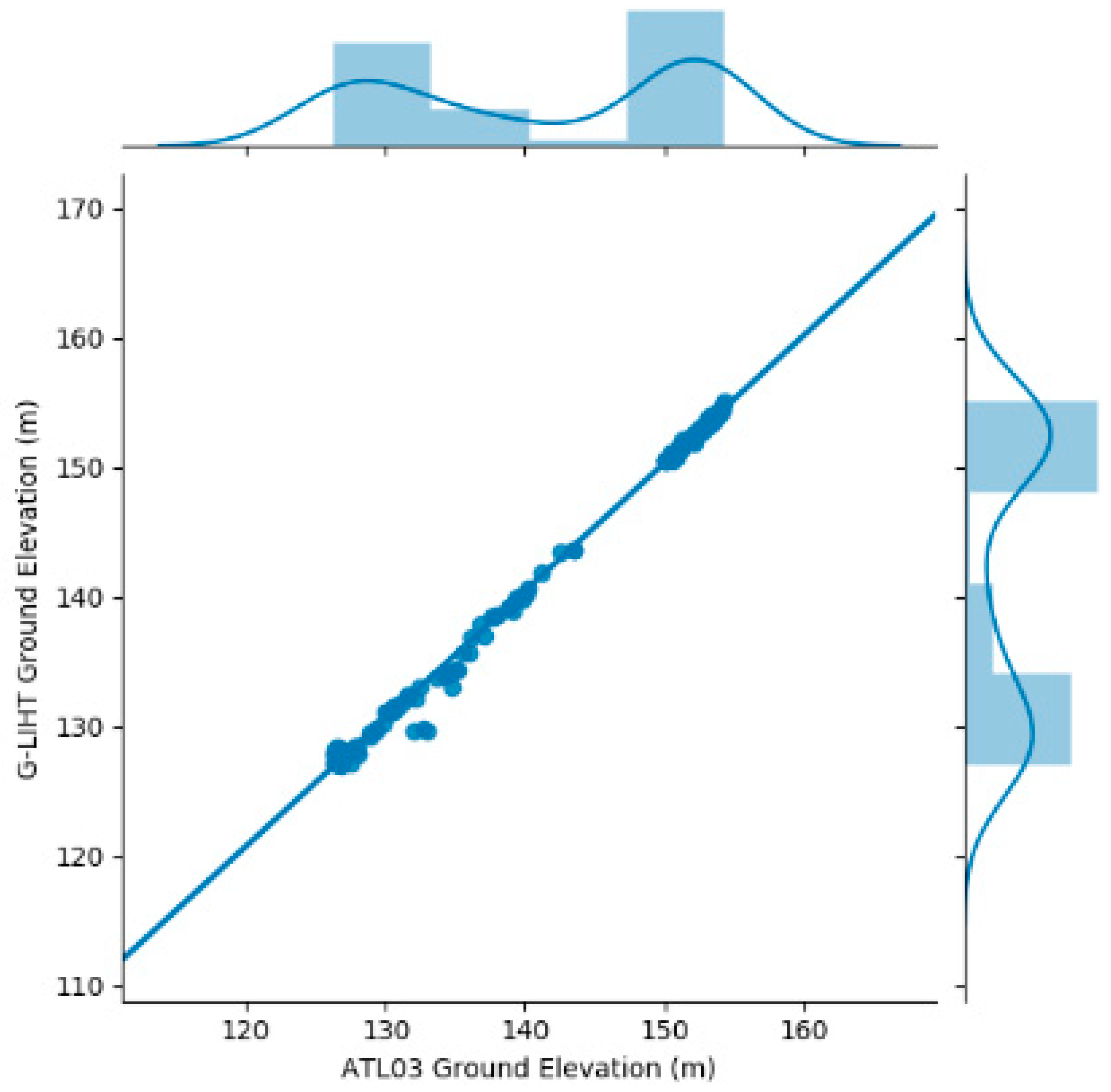
The estimated ground topography for different intensity beams shows significant agreement with the reference DTM elevations. For the weak beam and strong beam, the mean R2 values are 1, the ME values are 0.33 m and 0.27 m, and the RMSE values are 0.76 m and 0.74 m, respectively. The correlation coefficient of all types is greater than 0.89.
For the varying laser intensities in this data set, the statistical indicators for the strong beam performed better than that of weak beam with the lower RMSE (RMSEstrong beam = 0.74 m and RMSEweak beam = 0.76 m), lower MAE (MAEstrong beam = 0.51 m and MAEweak beam = 0.54 m), lower ME (ME strong beam = 0.33 m and ME weak beam = 0.27 m), and higher correlation coefficient. A possible reason is that the weak beam channel has fewer signal photons compared to the strong channel, making measuring ground topography in forested terrain using the weak beam more difficult. Using a strong beam, ATLAS could produce more signal photons than under the weak beam. The laser intensity ratio of strong beam to weak beam is 4:1. Depending upon the surface reflectance and atmospheric conditions, up to 16 photons per outgoing shot could be detected for the strong beam, while the weak beam could detect only 4 photons. However, the strong and weak beams can both provide useable data for measuring ground topography in forested terrain.
To further explore the influence of laser intensities on elevation errors, we calculated three correlation coefficients between tx_pulse_energy parameters and elevation errors (Table 6). For all the data, the correlation coefficients for the elevation errors and tx_pulse_energy parameters are greater than 0.5. In addition, the Spearman correlation coefficient values for the various laser intensities are greater than 0.74, indicating there is a significant correlation between the tx_pulse_energy parameters and elevation error. However, this contribution only explores the correlation between tx_pulse_energy and elevation error for a laser intensity ranging from 0.02 mJ to 0.09 mJ. Future studies with the tx_pulse_energy parameters will need to perform a more detailed analysis on the effect of tx_pulse_energy on elevation error.
Compared to the forested terrain ground topography estimation method in proposed by Neuenschwander et al. [37], higher R2 values and lower RMSE values were observed in the strong beam mode and weak beam mode. However, this study proposes a photon level which is different to the Neuenschwander et al. method [37], which notes that the result of a photon subset using a strong beam and a weak beam can reasonably explain the ground topography in the forest study area.

4.2. Retrieved Ground Topography in Forested Terrain Elevation with Different Laser Pointing Angles

The mean statistical indicators for the different laser pointing angles are listed in Table 7 and the correlation coefficient statistics between tx_pulse_skew_est, tx_pulse_width_lower, tx_pulse_width_upper parameters and the elevation errors of ATLAS data are listed in Table 8.
The estimated ground topography in forested terrain using different laser pointing angles shows strong agreement with the reference DTMG-LiHT elevations, as demonstrated by the R2 values equaling 1.00 and the RMSE values less than 0.92 m.
Results indicated that the gt1 channel pointing (R2gt1 channel = 1.00, RMSEgt1 channel=0.62 m, MAE gt1 channel = 0.4m) performed better than gt2 channel pointing (R2gt2 channel = 1.00, RMSEgt2 channel = 0.92 m, MAE gt2 channel = 0.62m) and gt3 channel pointing (R2gt3 channel = 1.00, RMSEgt3 channel = 0.71 m, MAE gt3 channel = 0.56m), which was due to several hardware reasons. On one hand, the gt1 channel could achieve more effective forested terrain signal photons than other channels in the study area. More signal photons can give a clearer depiction of ground topography in forested terrain. On the other hand, the photon rates of the gt1 and gt3 channels are higher than the gt2 channel, which is consistent with the description of the different laser pointing angles [46].
To further explore the influence of laser pointing angles on elevation error, we calculated three correlation coefficients between tx_pulse_skew_est, tx_pulse_width_lower, tx_pulse_width_upper parameters and elevation error. In the ATL03 Algorithm Theoretical Basis Document (ATBD), these parameters may be related to the laser pointing angles. The quantitative results of the correlation coefficients are summarized in Table 8. For all the data, the mean correlation coefficients for the elevation errors are less than 0.20. There is no significant correlation between the tx_pulse_skew_est, tx_pulse_width_lower, tx_pulse_width_upper parameters and the elevation error. However, this contribution only explores the correlation between tx_pulse_skew_est, tx_pulse_width_lower, tx_pulse_width_upper and the elevation error. Future studies needed to analyze other laser pointing angles parameters’ relative elevation errors.
The results of this contribution performed better than that proposed by Neuenschwander et al. [37] (R2 = 0.99, RMSE = 0.85), which notes that the result of a photon subset using different laser pointing angles can reasonably explain the ground topography in the study area.

4.3. Retrieved Ground Topography in Forested Terrain Elevation with ATLAS

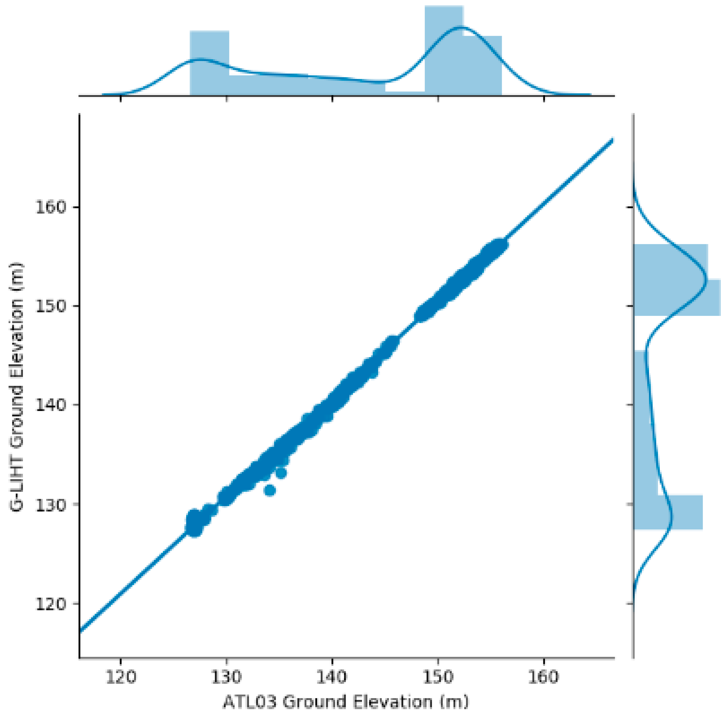
Most optical remote sensing systems could provide images of the horizontal distribution of ground topography, and the product generally follows the uppermost surface elevation (i.e., representing a digital surface model, DSM). However, the optical remote sensing images do not provide detailed information on the vertical distribution of ground topography in forested terrain, without regard to whether the surface is comprised of forest or not [5,6,47]. In contrast, the LiDAR photon counting signature from ICESat-2/ATLAS could provide a direct depiction for ground topography in forested terrain. In this contribution, the close correspondence between the ATLAS and G-LiHT (R2 = 1.00, RMSE = 0.75 m) confirms that the received photon data are an accurate representation of the ground topography forested terrain elevation within the ATLAS footprints. As a comparison, in areas of low relief (slope ≤ 5°) and middle dense tree cover (tree cover = 20%–40%), the mean and standard deviation of elevation differences between the ICESat/GLAS centroid and SRTM are −2.48 ± 4.04 m [48]. Thus, the estimation of ground topography for forest-covered areas is able to be accomplished with ICESat-2/ATLAS.
The results from this contribution indicate that the ground topography in forested terrain elevation can be estimated using photon data from ICESat-2/ATLAS multi-channel. We were able to retrieve terrain elevation successfully in forest-covered areas. Prior work showing the correlation between spaceborne LiDAR-measured canopy height and ground topography in forested terrain [21,22,23], which provide confidence that ICESat-2/ATLAS photon data in combination with GEDI data can substantially contribute to a global inventory of forest biomass. The work also provides insights for future work to improve the accuracy of the canopy height estimations.

5. Conclusions

In this contribution, ICESat-2 data is used to measure ground topography in forested terrain using different channels. The retrieved ground topography was validated by experiments with G-LiHT airborne data at different laser pointing angles and laser intensity types on the same route. Based on the results, the following conclusions can be drawn:
(1) Both qualitative and quantitative results indicate that at all laser intensities and laser pointing types resulted in a mean R2 = 1.00 and mean RMSE = 0.75 m, highlighting the ability of the ATL03 and ATL08 data to retrieve ground elevations.
(2) A significant correlation exists between the tx_pulse_energy parameters and elevation error. There is no significant correlation between tx_pulse_skew_est, tx_pulse_width_lower, tx_pulse_width_upper parameters and elevation error.
These conclusions give valuable insight into the ground topography in forested terrain using different ATLAS channels. Nevertheless, there are still many issues to be addressed in the future. Since ATLAS data is still in the research stage, we only considered the effects of laser pointing angles and laser intensity on retrieving ground topography. Other factors (e.g., canopy height, canopy cover, etc.) influencing the results were not considered. Therefore, the effects of other factors on retrieving ground topography over forested terrain using ATLAS data should be thoroughly examined in the future.

Author Contributions

J.H., Y.X. and L.Q. conceived and designed the experiments; J.H. performed the experiments; J.H. and Y.X. analyzed the data; L.Q. contributed materials; J.H., Y.X. and A.G. wrote the paper; Y.X. secured funding for the project; A.G. polished the language of the manuscript. All authors have read and agreed to the published version of the manuscript.

Funding

This work is supported by the National Key R&D Program of China (Grant Number: 2017YFD0600904), the Fundamental Research Funds for the Central Universities (Grant Number:2572019AB18), and the Key Laboratory of Satellite Mapping Technology and Application, National Administration of Surveying, Mapping and Geoinformation (KLSMTA-201706).

Acknowledgments

We thank the editor and anonymous reviewers for reviewing our paper.

Conflicts of Interest

The authors declare no conflict of interest.

References

  1. Thom, D.; Keeton, W.S. Stand structure drives disparities in carbon storage in northern hardwood-conifer forests. For. Ecol. Manag. 2019, 442, 10–20. [Google Scholar] [CrossRef] [Green Version]
  2. Ferreira, A.C.; Bezerra, L.E.A.; Cascon, H.M. Aboveground carbon stock in a restored neotropical mangrove: Influence of management and brachyuran crab assemblage. Wetl. Ecol. Manag. 2019, 27, 223–242. [Google Scholar] [CrossRef]
  3. Quegan, S.; le Toan, T.; Chave, J.; Dall, J.; Exbrayat, J.F.; Minh, D.H.T.; Lomas, M.; d’Alessandro, M.M.; Paillou, P.; Papathanassiouet, K.; et al. The European Space Agency BIOMASS mission: Measuring forest above-ground biomass from space. Remote Sens. Environ. 2019, 227, 44–60. [Google Scholar] [CrossRef] [Green Version]
  4. Ni, W.; Zhang, Z.; Sun, G.; Liu, Q. Modeling the Stereoscopic Features of Mountainous Forest Landscapes for the Extraction of Forest Heights from Stereo Imagery. Remote Sens. 2019, 11, 1222. [Google Scholar] [CrossRef] [Green Version]
  5. Hu, T.; Su, Y.; Xue, B.; Liu, J.; Zhao, X.; Fang, J.; Guo, Q. Mapping Global Forest Aboveground Biomass with Spaceborne LiDAR, Optical Imagery, and Forest Inventory Data. Remote Sens. 2016, 8, 565. [Google Scholar] [CrossRef] [Green Version]
  6. Wang, S.; Ren, Z.; Wu, C.; Lei, Q.; Gong, W.; Ou, Q.; Zhang, H.; Ren, G.; Li, C. DEM generation from Worldview-2 stereo imagery and vertical accuracy assessment for its application in active tectonics. Geomorphology 2019, 336, 107–118. [Google Scholar] [CrossRef]
  7. Yu, Y.; Yang, X.G.; Fan, W.Y. Estimates of forest structure parameters from GLAS data and multi-angle imaging spectrometer data. Int. J. Appl. Earth Obs. Geoinf. 2015, 38, 65–71. [Google Scholar] [CrossRef]
  8. Zhao, F.; Yang, X.Y.; Strahler, A.H.; Schaaf, C.L.; Yao, T.; Wang, Z.S.; Román, M.O.; Woodcock, C.E.; Ni-Meister, W.; Jupp, D.L.B.; et al. A comparison of foliage profiles in the Sierra National Forest obtained with a full-waveform under-canopy EVI lidar system with the foliage profiles obtained with an airborne full-waveform LVIS lidar system. Remote Sens. Environ. 2013, 136, 330–341. [Google Scholar] [CrossRef] [Green Version]
  9. Bouvier, M.; Durrieu, S.; Fournier, R.A.; Renaud, J.P. Generalizing predictive models of forest inventory attributes using an area-based approach with airborne LiDAR data. Remote Sens. Environ. 2015, 156, 322–334. [Google Scholar] [CrossRef]
  10. Dandois, J.P.; Ellis, E.C. High spatial resolution three-dimensional mapping of vegetation spectral dynamics using computer vision. Remote Sens. Environ. 2013, 136, 259–276. [Google Scholar] [CrossRef] [Green Version]
  11. Disney, M.; Burt, A.; Calders, K.; Schaaf, C.; Stovall, A. Innovations in Ground and Airborne Technologies as Reference and for Training and Validation: Terrestrial Laser Scanning (TLS). Surv. Geophys. 2019, 40, 937–958. [Google Scholar] [CrossRef] [Green Version]
  12. Disney, M. Terrestrial LiDAR: A three-dimensional revolution in how we look at trees. N. Phytol. 2019, 222, 1736–1741. [Google Scholar] [CrossRef] [PubMed] [Green Version]
  13. Wijesingha, J.; Moeckel, T.; Hensgen, F.; Wachendorf, M. Evaluation of 3D point cloud-based models for the prediction of grassland biomass. Int. J. Appl. Earth Obs. Geoinf. 2019, 78, 352–359. [Google Scholar] [CrossRef]
  14. Schneider, F.D.; Kükenbrink, D.; Schaepman, M.E.; Schimel, D.S.; Morsdorf, F. Quantifying 3D structure and occlusion in dense tropical and temperate forests using close-range LiDAR. Agric. For. Meteorol. 2019, 268, 249–257. [Google Scholar] [CrossRef]
  15. Bakx, T.R.; Koma, Z.; Seijmonsbergen, A.C.; Kissling, W.D. Use and categorization of Light Detection and Ranging vegetation metrics in avian diversity and species distribution research. Divers. Distrib. 2019, 25, 1045–1059. [Google Scholar] [CrossRef] [Green Version]
  16. Zwally, H.J.; Schutz, B.; Abdalati, W.; Abshire, J.; Bentley, C.; Brenner, A.; Bufton, J.; Dezio, J.; Hancock, D.; Harding, D.; et al. ICESat’s laser measurements of polar ice, atmosphere, ocean, and land. J. Geodyn. 2002, 34, 405–445. [Google Scholar] [CrossRef] [Green Version]
  17. Kellner, J.R.; Armston, J.; Birrer, M.; Cushman, K.C.; Duncanson, L.; Eck, C.; Falleger, C.; Imbach, B.; Král, K.; Krůček, M.; et al. New Opportunities for Forest Remote Sensing Through Ultra-High-Density Drone Lidar. Surv. Geophys. 2019, 40, 959–977. [Google Scholar] [CrossRef] [Green Version]
  18. Popescu, S.C.; Zhou, T.; Nelson, R.; Neuenschwander, A.; Sheridan, R.; Narine, L.; Walsh, K.M. Photon counting LiDAR: An adaptive ground and canopy height retrieval algorithm for ICESat-2 data. Remote Sens. Environ. 2018, 208, 154–170. [Google Scholar] [CrossRef]
  19. Wang, Y.; Ni, W.; Sun, G.; Chi, H.; Zhang, Z.; Guo, Z. Slope-adaptive waveform metrics of large footprint lidar for estimation of forest aboveground biomass. Remote Sens. Environ. 2019, 224, 386–400. [Google Scholar] [CrossRef]
  20. Harding, D.J.; Carabajal, C.C. ICESat waveform measurements of within footprint topographic relief and vegetation vertical structure. Geophys. Res. Lett. 2005, 32, L21S10. [Google Scholar] [CrossRef] [Green Version]
  21. Lefsky, M.A.; Harding, D.J.; Keller, M.; Cohen, W.B.; Carabajal, C.C.; Espirito-Santo, F.D.B.; Hunter, M.O.; de Oliveira, R., Jr. Estimates of forest canopy height and above ground biomass using ICESat. Geophys. Res. Lett. 2005, 32, L22S02. [Google Scholar] [CrossRef] [Green Version]
  22. Chen, Q. Assessment of terrain elevation derived from satellite laser altimetry over mountainous forest areas using airborne lidar data. ISPRS J. Photogramm. Remote Sens. 2010, 65, 111–122. [Google Scholar] [CrossRef]
  23. Fang, Z.; Cao, C.X. Estimation of Forest Canopy Height Over Mountainous Areas Using Satellite Lidar. IEEE J. Sel. Top. Appl. Earth Obs. Remote Sens. 2014, 7, 3157–3166. [Google Scholar] [CrossRef]
  24. Lee, S.; Ni-Meister, W.; Yang, W.; Chen, Q. Physically based vertical vegetation structure retrieval from ICESat data: Validation using LVIS in White Mountain National Forest, New Hampshire, USA. Remote Sens. Environ. 2011, 115, 2776–2785. [Google Scholar] [CrossRef]
  25. Claudia, H.; Christiane, S. Influence of Surface Topography on ICESat/GLAS Forest Height Estimation and Waveform Shape. Remote Sens. 2012, 4, 2210–2235. [Google Scholar] [CrossRef] [Green Version]
  26. Saarela, S.; Holm, S.; Healey, S.P.; Andersen, H.-E.; Petersson, H.; Prentius, W.; Patterson, P.L.; Næsset, E.; Gregoire, T.G.; Ståhl, G. Generalized Hierarchical Model-Based Estimation for Aboveground Biomass Assessment Using GEDI and Landsat Data. Remote Sens. 2018, 10, 1832. [Google Scholar] [CrossRef] [Green Version]
  27. Markus, T.; Neumann, T.; Martino, A.; Abdalati, W.; Brunt, K.; Csatho, B.; Farrell, S.; Fricker, H.; Gardner, A.; Harding, D.; et al. The Ice, Cloud, and land Elevation Satellite-2 (ICESat-2): Science requirements, concept, and implementation. Remote Sens. Environ. 2017, 190, 260–273. [Google Scholar] [CrossRef]
  28. Brunt, K.M.; Neumann, T.A.; Walsh, K.M.; Markus, T. Determination of Local Slope on the Greenland Ice Sheet Using a Multibeam Photon-Counting Lidar in Preparation for the ICESat-2 Mission. IEEE Geosci. Remote Sens. Lett. 2014, 11, 935–939. [Google Scholar] [CrossRef] [Green Version]
  29. Magruder, L.A.; Brunt, K.M. Performance Analysis of Airborne Photon Counting Lidar Data in Preparation for the ICESat-2 Mission. IEEE Trans. Geosci. Remote Sens. 2018, 56, 2911–2918. [Google Scholar] [CrossRef]
  30. Ma, Y.; Li, S.; Zhang, W.; Zhang, Z.; Liu, R.; Wang, X.H. Theoretical ranging performance model and range walk error correction for photon counting lidars with multiple detectors. Opt. Express 2018, 26, 15924–15934. [Google Scholar] [CrossRef]
  31. Li, S.; Zhang, Z.; Ma, Y.; Zeng, H.; Zhao, P.; Zhang, W. Ranging performance models based on negative-binomial (NB) distribution for photon-counting lidars. Opt. Express 2019, 27, A861–A877. [Google Scholar] [CrossRef] [PubMed]
  32. Ma, Y.; Liu, R.; Li, S.; Zhang, W.; Yang, F.; Su, D. Detecting the ocean surface from the raw data of the MABEL photon-counting lidar. Opt. Express 2018, 26, 24752–24762. [Google Scholar] [CrossRef] [PubMed]
  33. Neuenschwander, A.L.; Magruder, L.A. The Potential Impact of Vertical Sampling Uncertainty on ICESat-2/ATLAS Terrain and Canopy Height Retrievals for Multiple Ecosystems. Remote Sens. 2016, 8, 1039. [Google Scholar] [CrossRef] [Green Version]
  34. Abdalati, W.; Zwally, H.J.; Bindschadler, R.; Csatho, B.; Farrell, S.L.; Fricker, H.A.; Harding, D.; Kwok, R.; Lefsky, M.; Markus, T.; et al. ICESat-2 Laser Altimetry Mission. Proc. IEEE 2010, 98, 735–751. [Google Scholar] [CrossRef]
  35. Nie, S.; Wang, C.; Xi, X.; Luo, S.; Li, G.; Tian, J.; Wang, H. Estimating the vegetation canopy height using micro-pulse photon-counting LiDAR data. Opt. Express 2018, 26, A520–A540. [Google Scholar] [CrossRef]
  36. Narine, L.L.; Popescu, S.C.; Malambo, L. Synergy of ICESat-2 and Landsat for Mapping Forest Aboveground Biomass with Deep Learning. Remote Sens. 2019, 11, 1503. [Google Scholar] [CrossRef]
  37. Neuenschwander, A.L.; Magruder, L.A. Canopy and Terrain Height Retrievals with ICESat-2: A First Look. Remote Sens. 2019, 11, 1721. [Google Scholar] [CrossRef] [Green Version]
  38. Wang, C.; Zhu, X.; Nie, S.; Xi, X.; Li, D.; Zheng, W.; Chen, S. Ground elevation accuracy verification of ICESat-2 data: A case study in Alaska, USA. Opt. Express. 2019, 27, 38168–38179. [Google Scholar] [CrossRef]
  39. Neumann, T.; Brenner, A.; Hancock, D.; Robbins, J.; Saba, J.; Harbeck, K.; Gibbons, A. ICE, CLOUD, and Land Elevation Satellite-2(ICESat-2) Project Algorithm Theoretical Basis Document (ATBD) for Global Geolocated Photons ATL03; National Aeronautics and Space Administration: Washington, DC, USA; Goddard Space Flight Centre: Greenbelt, MD, USA, 2018. [Google Scholar]
  40. Harrington, T.B.; Edwards, M.B. Understory vegetation, resource availability, and litterfall responses to pine thinning and woody vegetation control in longleaf pine plantations. Can. J. For. Res. 1999, 29, 1055–1064. [Google Scholar] [CrossRef]
  41. Huang, J.P.; Xing, Y.Q.; You, H.T.; Qin, L.; Tian, J.; Ma, J.M. Particle Swarm Optimization-Based Noise Filtering Algorithm for Photon Cloud Data in Forest Area. Remote Sens. 2019, 11, 980. [Google Scholar] [CrossRef] [Green Version]
  42. Neuenschwander, A.; Popescu, S.; Nelson, R.; Harding, D.; Pitts, K.; Robbins, J.; Pederson, D.; Sheridan, R. ICE, CLOUD, and Land Elevation Satellite (ICESat-2) Algorithm Theoretical Basis Document (ATBD) for Land- Vegetation Along-Track Products; National Aeronautics and Space Administration: Washington, DC, USA; Goddard Space Flight Centre: Greenbelt, MD, USA, 2019. [Google Scholar]
  43. Neumann, T.; Brenner, A.; Hancock, D.; Luthcke, S.; Lee, J.; Robbins, J.; Harbeck, K.; Saba, J.; Brunt, K. ATLAS/ICESat-2 L2A Global Geolocated Photon Data, Version 2; NSIDC National Snow and Ice Data Center: Boulder, CO, USA, 2019. [Google Scholar]
  44. Cook, B.D.; Corp, L.A.; Nelson, R.F.; Middleton, E.M.; Morton, D.C.; McCorkel, J.T.; Masek, J.G.; Ranson, K.J.; Ly, V.; Montesano, P.M. NASA Goddard’s LiDAR, Hyperspectral and Thermal (G-LiHT) Airborne Imager. Remote Sens. 2013, 5, 4045–4066. [Google Scholar] [CrossRef] [Green Version]
  45. Chen, B.; Pang, Y.; Li, Z.; North, P.; Rosette, J.; Sun, G.; Suárez, J.; Bye, I.; Lu, H. Potential of Forest Parameter Estimation Using Metrics from Photon Counting LiDAR Data in Howland Research Forest. Remote Sens. 2019, 11, 856. [Google Scholar] [CrossRef] [Green Version]
  46. Kwok, R.; Markus, T.; Kurtz, N.T.; Petty, A.A.; Farrell, T.A.N.S.L.; Cunningham, G.F.; Hancock, D.W.; Ivanoff, A.; Wimert, J.T. Surface Height and Sea Ice Freeboard of the Arctic Ocean From ICESat-2: Characteristics and Early Results. J. Geophys. Res. Oceans 2019, 124. [Google Scholar] [CrossRef]
  47. Meddens, A.J.; Vierling, L.A.; Eitel, J.U.; Jennewein, J.S.; White, J.C.; Wulder, M.A. Developing 5 m resolution canopy height and digital terrain models from WorldView and ArcticDEM data. Remote Sens. Environ. 2018, 218, 174–188. [Google Scholar] [CrossRef]
  48. Carabajal, C.C.; Harding, D.J. ICESat validation of SRTM C-band digital elevation models. Geophys. Res. Lett. 2005, 32, L22S01. [Google Scholar] [CrossRef] [Green Version]
Figure 1. Location of the study area at the national and state levels. Figure 1 shows a part of the study site using an image of a USA map. The left part of the image shows the location of the study area in the USA, the right part shows it relative to South Carolina.
Remotesensing 12 02084 g001
Figure 2. (a) The location of gt3r and gt3l data in site 1, City of Aiken, USA. gt3r photons (yellow) and gt3l photons (red) show the location of the Ice, Cloud, and Land Elevation Satellite-2 (ICESat-2) track in Google Earth for context [43]. This illustration only includes signal photons (signal_conf_ph=4) and is located in City of Aiken, USA. (b): Profile of ATL03 photons from the weak beam (gt3l). This data was collected on 26 December 2018 at 05:31. (c): Profile of ATL03 photons from the strong beam (gt3r), which has a greater number of signal photons above the surface than in gt3l.
Remotesensing 12 02084 g002
Figure 3. (a): Trajectories of Advanced Topographic Laser Altimeter (ATLAS) data (green) and G-LiHT data (blue) depict the location of the study area NASA EARTHDATA. (b): G-LiHT data named AMIGACarb_Augusta_FIA_Sep2011_l16s597_DTM.tif as reference airborne data. (c): G-LiHT data named AMIGACarb_Augusta_FIA_Sep2011_l40s557_DTM.tif as reference airborne data.
Remotesensing 12 02084 g003
Figure 4. The flowchart of the analysis process.
Remotesensing 12 02084 g004
Figure 5. Two experimental data (a,b) sets in study area. The green dots on this figure are ATLAS footprints. The gray block is the G-LiHT Digital Terrain Model (DTM).
Remotesensing 12 02084 g005
Figure 6. A subset of the forested terrain ATL03 (gt3l) ground topography validation results from track ATL03_20181226053112_13530106_001_01. ATLAS photon data are shown as red dots. The ATLAS DTM (blue line) and the G-LiHT DTM (red line) are also shown.
Remotesensing 12 02084 g006
Figure 7. A subset of the forested terrain ATL03 (gt3r) ground topography validation results from track ATL03_20181226053112_13530106_001_01. The ATLAS photon data are shown as red dots. The ATLAS DTM (blue line) and the G-LiHT DTM (red line) are also shown.
Remotesensing 12 02084 g007
Figure 8. Scatterplot of ATL03 (gt3l) ground topography compared to G-LiHT DTM.
Remotesensing 12 02084 g008
Figure 9. Scatterplot of ATL03 (gt3r) ground topography compared to G-LiHT DTM.
Remotesensing 12 02084 g009
Table 1. The statistical indicators of global geolocated photon (ATL03) data [39].
ATL03 Product Parameter NameDescription
lat_phLatitude of each received photon. Computed from the ECF Cartesian coordinates of the bounce point.
lon_phLongitude of each received photon. Computed from the ECF Cartesian coordinates of the bounce point.
h_phHeight of each received photon, relative to the WGS-84 ellipsoid.
geoidGeoid height above WGS-84 reference ellipsoid (range −107 to 86 m).
delta_timeElapsed seconds from the ATLAS SDP GPS Epoch, corresponding to the transmit time of the reference photon.
signal_conf_phConfidence level associated with each photon event selected as signal. 0 = noise. 1 = added to allow for buffer but algorithm classifies as background; 2 = low; 3 = med; 4 = high).
sc_orientThis parameter tracks the spacecraft orientation between forward, backward and transitional flight modes.
tx_pulse_energyThe average transmit pulse energy, measured by the internal laser energy monitor, split into per-beam measurements.
tx_pulse_skew_estThe difference between the averages of the lower and upper threshold crossing times. This is an estimate of the transmit pulse skew.
tx_pulse_width_lowerThe average distance between the lower threshold crossing times measured by the Start Pulse Detector.
tx_pulse_width_upperThe average distance between the upper threshold crossing times measured by the Start Pulse Detector.
Table 2. The statistical indicators of land vegetation elevation (ATL08) product [42].
ATL08 Product Parameter NameDescription
classed_pc_flagLand Vegetation ATBD classification flag for each photon as either noise, ground, canopy, and top of canopy. 0 = noise, 1 = ground, 2 = canopy, or 3 = top of canopy.
classed_pc_indxThe unique identifier for tracing each ATL08 signal photon to the corresponding photon record on ATL03 is the segment_id, orbit, cycle, and classed_pc_indx.
ph_segment_idSegment ID of photons tracing back to specific 20 m segment_id on ATL03. The unique identifier for tracing each ATL08 signal photon to the photon on ATL03 is the segment_id, orbit, and classed_pc_indx. The unique identifier for tracing each ATL08 signal photon to the corresponding photon record on ATL03 is the segment_id, orbit, cycle, and classed_pc_indx.
Table 3. The Goddard’s LiDAR, Hyperspectral and Thermal imager (G-LiHT) product levels [44].
G-LiHT Product Product Level
Trajectory dataLevel 1
Classified return dataLevel 2
Above Ground Level (AGL) heightLevel 2
LiDAR returnsLevel 3
DTMLevel 3
Canopy Height Model (CHM)Level 3
Table 4. The statistical indicators of the various laser channels.
Different Laser ChannelsRMSE (m)MAE (m)R2ME (m)PearsonSpearmanKendall
gt1l0.690.351.00−0.051.000.990.92
gt1r0.550.451.000.271.000.990.92
gt2l0.800.671.000.591.000.960.84
gt2r1.030.580.990.041.000.990.93
gt3l0.780.601.000.451.000.990.93
gt3r0.640.521.000.491.000.990.94
Mean of channel0.750.531.000.301.000.980.91
Note: RMSE––root mean squared error; MAE––mean absolute error; R2––coefficient of determination; ME––mean error.
Table 5. Statistical indicators for different laser intensities.
Different Laser Intensities TypesRMSE (m)MAE(m)R2ME (m)PearsonSpearmanKendall
Weak beam0.76 0.54 1.00 0.33 1.00 0.98 0.89
Strong beam0.74 0.51 1.00 0.27 1.00 0.99 0.93
Table 6. Correlation coefficient statistics between tx_pulse_energy parameters and ATLAS data. error.
Different Laser Intensities TypesPearsonSpearmanKendall
Weak beam0.58 0.76 0.54
Strong beam0.59 0.74 0.51
Mean of different laser intensities Types0.59 0.75 0.53
Table 7. The statistical indicators for different laser pointing angles.
Different Laser ChannelsRMSE (m)MAE(m)R2ME (m)PearsonSpearmanKendall
gt10.62 0.40 1.00 0.11 1.00 0.99 0.92
gt20.92 0.62 1.00 0.31 1.00 0.97 0.88
gt30.71 0.56 1.00 0.47 1.00 0.99 0.93
Table 8. The correlation coefficient statistics between tx_pulse_skew_est, tx_pulse_width_lower, tx_pulse_width_upper parameters and the elevation errors of ATLAS data.
Statistical IndicatorsDifferent Laser Pointing AnglesPearsonSpearmanKendall
tx_pulse_skew_estgt10.12 0.05 0.04
gt20.11 0.21 0.12
gt30.15 0.15 0.11
Mean of different pointings0.13 0.14 0.09
tx_pulse_width_lowergt10.20 0.10 0.07
gt20.10 0.07 0.05
gt30.20 0.21 0.14
Mean of different pointings0.17 0.13 0.09
tx_pulse_width_uppergt10.24 0.31 0.23
gt20.09 0.12 0.09
gt30.11 0.13 0.09
Mean of different pointings0.15 0.19 0.14

