Effect of Lockdown Measures on Atmospheric Nitrogen Dioxide during SARS-CoV-2 in Spain

 , , and
Abstract
:
1. Introduction
2. Materials and Methods
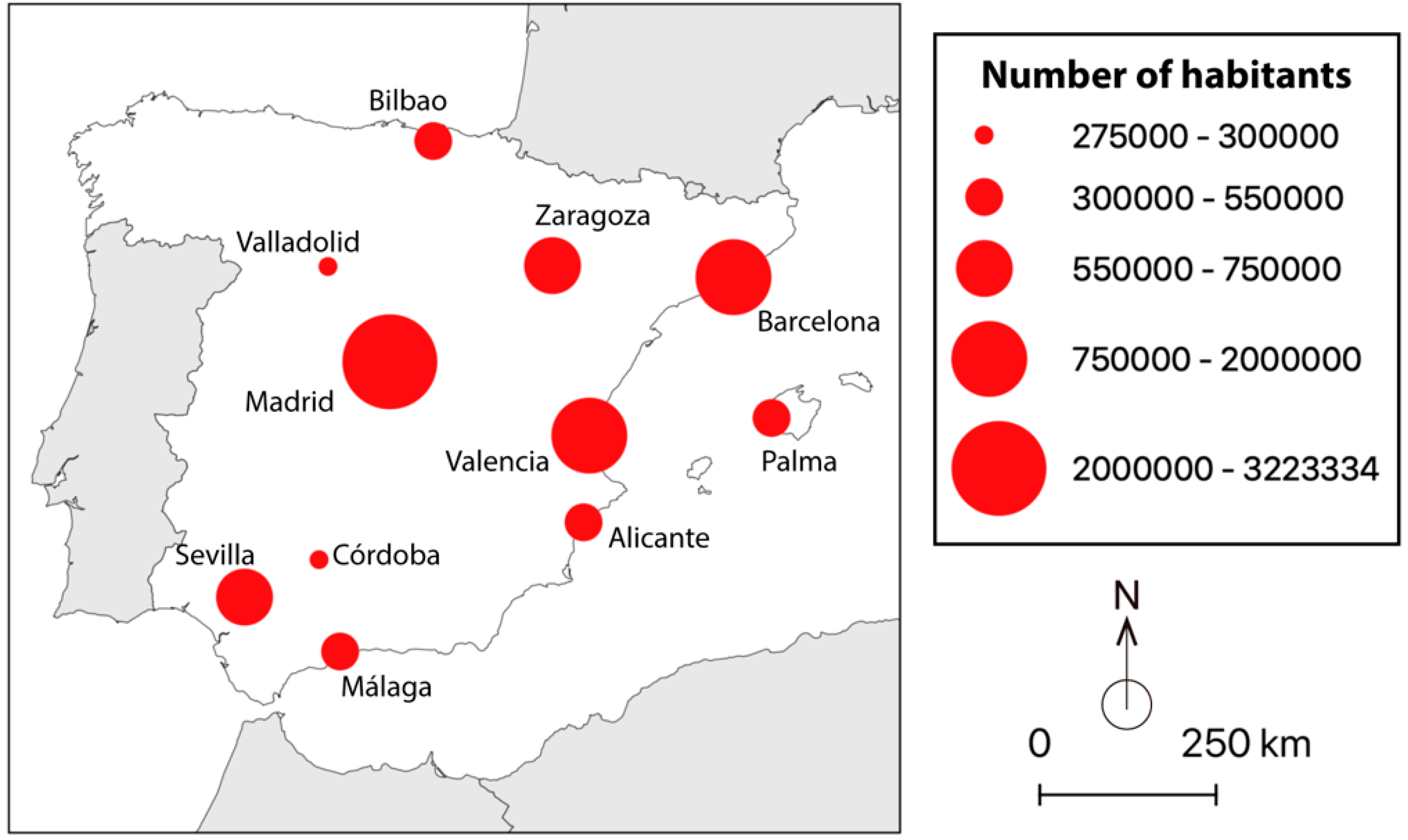
2.1. Study Area
2.2. Remote Sensing Image Collections
3. Results
4. Discussion
5. Conclusions
Author Contributions
Funding
Conflicts of Interest
References
- World Health Organization Air pollution. Available online: https://www.who.int/health-topics/air-pollution#ta (accessed on 25 May 2020).
- Gurjar, B.R.; Lelieveld, J. New Directions: Megacities and global change. AtmEn 2005, 39, 391–393. [Google Scholar] [CrossRef]
- CAI-Asia Center. Indonesia: Air Quality Profile; Clean Air Initiative for Asian Cities (CAI-Asia) Center: Pasig, Philippines, 2010. [Google Scholar]
- Khandelwal, S.; Goyal, R.; Kaul, N.; Mathew, A. Assessment of land surface temperature variation due to change in elevation of area surrounding Jaipur, India. Egypt. J. Remote Sens. Space Sci. 2018, 21, 87–94. [Google Scholar] [CrossRef]
- Dadhich, P.N.; Hanaoka, S. Spatial investigation of the temporal urban form to assess impact on transit services and public transportation access. Geo Spat. Inf. Sci. 2012, 15, 187–197. [Google Scholar] [CrossRef]
- Ravindra, K.; Mor, S.; Kamyotra, J.S.; Kaushik, C.P. Variation in Spatial Pattern of Criteria Air Pollutants Before and During Initial Rain of Monsoon. Environ. Monit. Assess. 2003, 87, 145–153. [Google Scholar] [CrossRef] [PubMed]
- Marsh, W.M.; Grossa, J., Jr. Environmental Geography: Science, Land Use, and Earth Systems, 2nd ed.; John Wiley and Sons: New York, NY, USA, 2002; ISBN 0471503967. [Google Scholar]
- Pasqua, L.A.; Damasceno, M.V.; Cruz, R.; Matsuda, M.; Martins, M.A.G.; Marquezini, M.V.; Lima-Silva, A.E.; Saldiva, P.H.N.; Bertuzzi, R. Exercising in the urban center: Inflammatory and cardiovascular effects of prolonged exercise under air pollution. Chemosphere 2020, 254, 126817. [Google Scholar] [CrossRef]
- Shmuel, S.; White, A.J.; Sandler, D.P. Residential exposure to vehicular traffic-related air pollution during childhood and breast cancer risk. Environ. Res. 2017, 159, 257–263. [Google Scholar] [CrossRef]
- Kopnina, H. Vehicular air pollution and asthma: Implications for education for health and environmental sustainability. Local Environ. 2017, 22, 38–48. [Google Scholar] [CrossRef] [Green Version]
- Tang, G.; Zhao, P.; Wang, Y.; Gao, W.; Cheng, M.; Xin, J.; Li, X.; Wang, Y. Mortality and air pollution in Beijing: The long-term relationship. Atmos. Environ. 2017, 150, 238–243. [Google Scholar] [CrossRef]
- He, G.; Fan, M.; Zhou, M. The effect of air pollution on mortality in China: Evidence from the 2008 Beijing Olympic Games. J. Environ. Econ. Manag. 2016, 79, 18–39. [Google Scholar] [CrossRef]
- World Health Organization. WHO Air Quality Guidelines for Particulate Matter, Ozone, Nitrogen Dioxide and Sulfur Dioxide: Global Update 2005: Summary of Risk Assessment; World Health Organization: Geneva, Switzerland, 2006. [Google Scholar]
- European Union Directive 2008/50/EC of the European Parliament and of the Council of 21 May 2008 on ambient air quality and cleaner air for Europe. Off. J. Eur. Union 2008, 152, 1–44.
- Yebin, T.; Wei, H.; Xiaoliang, H.; Liuju, Z.; Shou-En, L.; Yi, L.; Lingzhen, D.; Yuanhang, Z.; Tong, Z. Estimated Acute Effects of Ambient Ozone and Nitrogen Dioxide on Mortality in the Pearl River Delta of Southern China. Environ. Health Perspect. 2012, 120, 393–398. [Google Scholar]
- MacIntyre, E.A.; Gehring, U.; Mölter, A.; Fuertes, E.; Klümper, C.; Krämer, U.; Quass, U.; Hoffmann, B.; Gascon, M.; Brunekreef, B.; et al. Air Pollution and Respiratory Infections during Early Childhood: An Analysis of 10 European Birth Cohorts within the ESCAPE Project. Environ. Health Perspect. 2014, 122, 107–113. [Google Scholar] [CrossRef] [PubMed]
- Hesterberg, T.W.; Bunn, W.B.; McClellan, R.O.; Hamade, A.K.; Long, C.M.; Valberg, P.A. Critical review of the human data on short-term nitrogen dioxide (NO2) exposures: Evidence for NO2 no-effect levels. Crit. Rev. Toxicol 2009, 39, 743–781. [Google Scholar] [CrossRef] [PubMed]
- Ilan, L.; Cristian, M.; Gang, L.; Julie, N.; Brook, J.R. Evaluating Multipollutant Exposure and Urban Air Quality: Pollutant Interrelationships, Neighborhood Variability, and Nitrogen Dioxide as a Proxy Pollutant. Environ. Health Perspect. 2014, 122, 65–72. [Google Scholar]
- Stieb, D.M.; Burnett, R.T.; Smith-Doiron, M.; Brion, O.; Shin, H.H.; Economou, V. A New Multipollutant, No-Threshold Air Quality Health Index Based on Short-Term Associations Observed in Daily Time-Series Analyses. J. Air Waste Manag. Assoc. 2008, 58, 435–450. [Google Scholar] [CrossRef] [PubMed] [Green Version]
- Filleul, L.; Rondeau, V.; Vandentorren, S.; Le Moual, N.; Cantagrel, A.; Annesi-Maesano, I.; Charpin, D.; Declercq, C.; Neukirch, F.; Paris, C.; et al. Twenty five year mortality and air pollution: Results from the French PAARC survey. Occup. Environ. Med. 2005, 62, 453–460. [Google Scholar] [CrossRef] [Green Version]
- Chen, X.; Zhang, L.; Huang, J.; Song, F.; Zhang, L.; Qian, Z.; Trevathan, E.; Mao, H.; Han, B.; Vaughn, M.; et al. Long-term exposure to urban air pollution and lung cancer mortality: A 12-year cohort study in Northern China. Sci. Total Environ. 2016, 571, 855–861. [Google Scholar] [CrossRef]
- Gauderman, W.J.; Avol, E.; Lurmann, F.; Kuenzli, N.; Gilliland, F.; Peters, J.; McConnell, R. Childhood Asthma and Exposure to Traffic and Nitrogen Dioxide. Epidemiology 2005, 16, 737–743. [Google Scholar] [CrossRef]
- Kowalska, M.; Skrzypek, M.; Kowalski, M.; Cyrys, J. Effect of NOx and NO2 Concentration Increase in Ambient Air to Daily Bronchitis and Asthma Exacerbation, Silesian Voivodeship in Poland. Int. J. Environ. Res. Public Health 2020, 17, 754. [Google Scholar] [CrossRef] [Green Version]
- Beelen, R.; Hoek, G.; Van Den Brandt, P.A.; Goldbohm, R.A.; Fischer, P.; Schouten, L.J.; Jerrett, M.; Hughes, E.; Armstrong, B.; Brunekreef, B. Long-Term Effects of Traffic-Related Air Pollution on Mortality in a Dutch Cohort (NLCS-AIR Study). Environ. Health Perspect. 2008, 116, 196–202. [Google Scholar] [CrossRef]
- Eum, K.-D.; Kazemiparkouhi, F.; Wang, B.; Manjourides, J.; Pun, V.; Pavlu, V.; Suh, H. Long-term NO2 exposures and cause-specific mortality in American older adults. Environ. Int. 2019, 124, 10–15. [Google Scholar] [CrossRef] [PubMed]
- Amorim, L.C.A.; Carneiro, J.P.; Cardeal, Z.L. An optimized method for determination of benzene in exhaled air by gas chromatography–mass spectrometry using solid phase microextraction as a sampling technique. J. Chromatogr. B 2008, 865, 141–146. [Google Scholar] [CrossRef] [PubMed]
- Ma, Y.; Richards, M.; Ghanem, M.; Guo, Y.; Hassard, J. Air pollution monitoring and mining based on sensor grid in London. Sensors 2008, 8, 3601–3623. [Google Scholar] [CrossRef] [PubMed]
- Richards, M.; Ghanem, M.; Osmond, M.; Guo, Y.; Hassard, J. Grid-based analysis of air pollution data. Ecol. Model. 2006, 194, 274–286. [Google Scholar] [CrossRef]
- Boubrima, A.; Bechkit, W.; Rivano, H. Optimal WSN Deployment Models for Air Pollution Monitoring. IEEE Trans. Wirel. Commun. 2017, 16, 2723–2735. [Google Scholar] [CrossRef] [Green Version]
- Patil, D.; Thanuja, T.C.; Melinamath, B.C. Air Pollution Monitoring System Using Wireless Sensor Network (WSN) BT-Data Management, Analytics and Innovation; Balas, V.E., Sharma, N., Chakrabarti, A., Eds.; Springer: Singapore, 2019; pp. 391–400. [Google Scholar]
- Yi, W.Y.; Lo, K.M.; Mak, T.; Leung, K.S.; Leung, Y.; Meng, M.L. A survey of wireless sensor network based air pollution monitoring systems. Sensors 2015, 15, 31392–31427. [Google Scholar] [CrossRef] [Green Version]
- Zheng, Z.; Yang, Z.; Wu, Z.; Marinello, F. Spatial Variation of NO2 and Its Impact Factors in China: An Application of Sentinel-5P Products. Remote Sens. 2019, 11, 1939. [Google Scholar] [CrossRef] [Green Version]
- Nate, S. Remote-Sensing Applications for Environmental Health Research. Environ. Health Perspect. 2014, 122, A268–A275. [Google Scholar]
- Burrows, J.P.; Weber, M.; Buchwitz, M.; Rozanov, V.; Ladstätter-Weißenmayer, A.; Richter, A.; DeBeek, R.; Hoogen, R.; Bramstedt, K.; Eichmann, K.-U.; et al. The Global Ozone Monitoring Experiment (GOME): Mission Concept and First Scientific Results. J. Atmos. Sci. 1999, 56, 151–175. [Google Scholar] [CrossRef]
- Bovensmann, H.; Burrows, J.P.; Buchwitz, M.; Frerick, J.; Noël, S.; Rozanov, V.V.; Chance, K.V.; Goede, A.P.H. SCIAMACHY: Mission Objectives and Measurement Modes. J. Atmos. Sci. 1999, 56, 127–150. [Google Scholar] [CrossRef] [Green Version]
- Callies, J.; Corpaccioli, E.; Eisinger, M.; Hahne, A.; Lefebvre, A. GOME-2-Metop’s second-generation sensor for operational ozone monitoring. ESA Bull. 2000, 102, 28–36. [Google Scholar]
- Levelt, P.F.; Van Den Oord, G.H.J.; Dobber, M.R.; Malkki, A.; Visser, H.; De Vries, J.; Stammes, P.; Lundell, J.O.V.; Saari, H. The ozone monitoring instrument. IEEE Trans. Geosci. Remote Sens. 2006, 44, 1093–1101. [Google Scholar] [CrossRef]
- Veefkind, J.P.; Aben, I.; McMullan, K.; Förster, H.; De Vries, J.; Otter, G.; Claas, J.; Eskes, H.J.; De Haan, J.F.; Kleipool, Q.; et al. TROPOMI on the ESA Sentinel-5 Precursor: A GMES mission for global observations of the atmospheric composition for climate, air quality and ozone layer applications. Remote Sens. Environ. 2012, 120, 70–83. [Google Scholar] [CrossRef]
- Griffin, D.; Zhao, X.; McLinden, C.A.; Boersma, F.; Bourassa, A.; Dammers, E.; Degenstein, D.; Eskes, H.; Fehr, L.; Fioletov, V.; et al. High-Resolution Mapping of Nitrogen Dioxide With TROPOMI: First Results and Validation Over the Canadian Oil Sands. Geophys. Res. Lett. 2019, 46, 1049–1060. [Google Scholar] [CrossRef] [Green Version]
- Lamsal, L.N.; Duncan, B.N.; Yoshida, Y.; Krotkov, N.A.; Pickering, K.E.; Streets, D.G.; Lu, Z.U.S. NO2 trends (2005–2013): EPA Air Quality System (AQS) data versus improved observations from the Ozone Monitoring Instrument (OMI). Atmos. Environ. 2015, 110, 130–143. [Google Scholar] [CrossRef]
- Van Geffen, J.H.G.M.; Eskes, H.J.; Boersma, K.F.; Maasakkers, J.D.; Veefkind, J.P. TROPOMI ATBD of the Total and Tropospheric NO2 Data Products. Minist. Infrastruct. Water Manag. 2019. Available online: https://sentinel.esa.int/documents/247904/2476257/Sentinel-5P-TROPOMI-ATBD-NO2-data-products (accessed on 10 January 2020).
- Curier, R.L.; Kranenburg, R.; Segers, A.J.S.; Timmermans, R.M.A.; Schaap, M. Synergistic use of OMI NO2 tropospheric columns and LOTOS–EUROS to evaluate the NOx emission trends across Europe. Remote Sens. Environ. 2014, 149, 58–69. [Google Scholar] [CrossRef]
- Castellanos, P.; Boersma, K.F. Reductions in nitrogen oxides over Europe driven by environmental policy and economic recession. Sci. Rep. 2012, 2, 265. [Google Scholar] [CrossRef]
- Ghude, S.D.; Pfister, G.G.; Jena, C.; Van Der A, R.J.; Emmons, L.K.; Kumar, R. Satellite constraints of nitrogen oxide (NOx) emissions from India based on OMI observations and WRF-Chem simulations. Geophys. Res. Lett. 2013, 40, 423–428. [Google Scholar] [CrossRef]
- Streets, D.G.; Canty, T.; Carmichael, G.R.; De Foy, B.; Dickerson, R.R.; Duncan, B.N.; Edwards, D.P.; Haynes, J.A.; Henze, D.K.; Houyoux, M.R.; et al. Emissions estimation from satellite retrievals: A review of current capability. Atmos. Environ. 2013, 77, 1011–1042. [Google Scholar] [CrossRef] [Green Version]
- Wang, S.W.; Zhang, Q.; Streets, D.G.; He, K.B.; Martin, R.V.; Lamsal, L.N.; Chen, D.; Lei, Y.; Lu, Z. Growth in NOx emissions from power plants in China: Bottom-up estimates and satellite observations. Atmos. Chem. Phys. 2012, 12, 4429. [Google Scholar] [CrossRef] [Green Version]
- Kim, S.-W.; Heckel, A.; McKeen, S.A.; Frost, G.J.; Hsie, E.-Y.; Trainer, M.K.; Richter, A.; Burrows, J.P.; Peckham, S.E.; Grell, G.A. Satellite-Observed U.S. Power Plant NOx Emission Reductions and Their Impact on Air Quality. Geophys. Res. Lett. 2006, 33. Available online: https://0-agupubs-onlinelibrary-wiley-com.brum.beds.ac.uk/doi/full/10.1029/2006GL027749 (accessed on 20 May 2020). [CrossRef] [Green Version]
- World Economic Forum The Global Risks Report 2020. 2020. Available online: https://www.weforum.org/reports/the-global-risks-report-2020 (accessed on 20 May 2020).
- Ye, Z.-W.; Yuan, S.; Yuen, K.-S.; Fung, S.-Y.; Chan, C.-P.; Jin, D.-Y. Zoonotic origins of human coronaviruses. Int. J. Biol. Sci. 2020, 16, 1686–1697. [Google Scholar] [CrossRef] [Green Version]
- Ahmad, T.; Khan, M.; Haroon, T.H.M.; Nasir, S.; Hui, J.; Bonilla-Aldana, D.K.; Rodriguez-Morales, A.J. COVID-19: Zoonotic aspects. Travel Med. Infect. Dis. 2020. [Google Scholar] [CrossRef] [PubMed]
- Mackenzie, J.S.; Chua, K.B.; Daniels, P.W.; Eaton, B.T.; Field, H.E.; Hall, R.A.; Halpin, K.; Johansen, C.A.; Kirkland, P.D.; Lam, S.K.; et al. Emerging viral diseases of Southeast Asia and the Western Pacific. Emerg. Infect. Dis. 2001, 7, 497–504. [Google Scholar] [CrossRef] [PubMed]
- Olsen, B.; Munster, V.J.; Wallensten, A.; Waldenström, J.; Osterhaus, A.D.M.E.; Fouchier, R.A.M. Global Patterns of Influenza a Virus in Wild Birds. Science 2006, 312, 384–388. [Google Scholar] [CrossRef] [PubMed] [Green Version]
- Fergus, R.; Fry, M.; Karesh, W.B.; Marra, P.P.; Newman, S.; Paul, E. Migratory Birds and Avian Flu. Science 2006, 312, 845–846. [Google Scholar] [CrossRef]
- Petersen, L.R.; Marfin, A.A. Shifting Epidemiology of Flaviviridae. J. Travel Med. 2008, 12, s3–s11. [Google Scholar] [CrossRef] [Green Version]
- Leviston, Z.; Leitch, A.; Greenhill, M.; Leonard, R.; Walker, I. Australians’ Views of Climate Change. Canberra CSIRO 2011. Available online: https://www.researchgate.net/profile/Anne_Leitch/publication/255960321_Australians’_Views_of_Climate_Change/links/00b49520f2ef390d88000000/Australians-Views-of-Climate-Change.pdf (accessed on 20 May 2020).
- Price, J.C.; Walker, I.A.; Boschetti, F. Measuring cultural values and beliefs about environment to identify their role in climate change responses. J. Environ. Psychol. 2014, 37, 8–20. [Google Scholar] [CrossRef]
- Van Der Linden, S.L.; Leiserowitz, A.A.; Feinberg, G.D.; Maibach, E.W. The Scientific Consensus on Climate Change as a Gateway Belief: Experimental Evidence. PLoS ONE 2015, 10, e0118489. [Google Scholar] [CrossRef] [Green Version]
- Callaway, E. Time to use the p-word? Coronavirus enter dangerous new phase. Nature 2020, 579, 10–38. [Google Scholar] [CrossRef]
- Remuzzi, A.; Remuzzi, G. COVID-19 and Italy: What next? Lancet 2020, 395, 1225–1228. [Google Scholar] [CrossRef]
- Hou, C.; Chen, J.; Zhou, Y.; Hua, L.; Yuan, J.; He, S.; Guo, Y.; Zhang, S.; Jia, Q.; Zhao, C.; et al. The effectiveness of quarantine of Wuhan city against the Corona Virus Disease 2019 (COVID-19): A well-mixed SEIR model analysis. J. Med. Virol. 2020, 92, 841–848. [Google Scholar] [CrossRef] [PubMed] [Green Version]
- Lau, H.; Khosrawipour, V.; Kocbach, P.; Mikolajczyk, A.; Schubert, J.; Bania, J.; Khosrawipour, T. The positive impact of lockdown in Wuhan on containing the COVID-19 outbreak in China. J. Travel Med. 2020, 27. [Google Scholar] [CrossRef] [PubMed] [Green Version]
- Peto, J.; Alwan, N.A.; Godfrey, K.M.; Burgess, R.A.; Hunter, D.J.; Riboli, E.; Romer, P. Universal weekly testing as the UK COVID-19 lockdown exit strategy. Lancet 2020, 395, 1420–1421. [Google Scholar] [CrossRef]
- Gorelick, N.; Hancher, M.; Dixon, M.; Ilyushchenko, S.; Thau, D.; Moore, R. Google Earth Engine: Planetary-scale geospatial analysis for everyone. Remote Sens. Environ. 2017, 202, 18–27. [Google Scholar] [CrossRef]
- Eskes, H.J.; Eichmann, K.U. S5P Mission Performance Centre Nitrogen Dioxide [L2__NO2___]. 2019. Available online: https://sentinel.esa.int/documents/247904/3541451/Sentinel-5P-Nitrogen-Dioxide-Level-2-Product-Readme-File (accessed on 15 June 2020).
- Degraeuwe, B.; Pisoni, E.; Peduzzi, E.; De Meij, A.; Monforti-Ferrario, F.; Bodis, K.; Mascherpa, A.; Astorga-Llorens, M.; Thunis, P.; Vignati, E. Urban NO2 Atlas; Publications Office of the European Union: Brussels, Belgium, 2019; ISBN 978-92-76-10386-8. [Google Scholar]
- Harapan, H.; Itoh, N.; Yufika, A.; Winardi, W.; Keam, S.; Te, H.; Megawati, D.; Hayati, Z.; Wagner, A.L.; Mudatsir, M. Coronavirus disease 2019 (COVID-19): A literature review. J. Infect. Public Health 2020, 13, 667–673. [Google Scholar] [CrossRef]
- Ficetola, G.F.; Rubolini, D. Climate affects global patterns of COVID-19 early outbreak dynamics. MedRxiv 2020. [Google Scholar] [CrossRef] [Green Version]
- Zhu, Y.; Price, O.R.; Kilgallon, J.; Qi, Y.; Tao, S.; Jones, K.C.; Sweetman, A.J. Drivers of contaminant levels in surface water of China during 2000–2030: Relative importance for illustrative home and personal care product chemicals. Environ. Int. 2018, 115, 161–169. [Google Scholar] [CrossRef] [Green Version]
- Zhu, Y.; Zhan, Y.; Wang, B.; Li, Z.; Qin, Y.; Zhang, K. Spatiotemporally mapping of the relationship between NO2 pollution and urbanization for a megacity in Southwest China during 2005–2016. Chemosphere 2019, 220, 155–162. [Google Scholar] [CrossRef]
- De Tráfico, D.G.; Del, I.M. Evolución del Tráfico por el efecto COVID-19. Available online: http://www.dgt.es/Galerias/covid-19/Evolucion-Intensidades-dia-02-04-2020-Periodo-Coronavirus.pdf (accessed on 9 May 2020).
- Banister, D. Energy, quality of life and the environment: The role of transport. Transp. Rev. 1996, 16, 23–35. [Google Scholar] [CrossRef]
- Camagni, R.; Gibelli, M.C.; Rigamonti, P. Urban mobility and urban form: The social and environmental costs of different patterns of urban expansion. Ecol. Econ. 2002, 40, 199–216. [Google Scholar] [CrossRef]
- Ambarwati, L.; Verhaeghe, R.; Van Arem, B.; Pel, A.J. The influence of integrated space–transport development strategies on air pollution in urban areas. Transp. Res. Part D Transp. Environ. 2016, 44, 134–146. [Google Scholar] [CrossRef]


| Month | 2019 | 2020 |
|---|---|---|
| January | 426 | 424 |
| February | 382 | 379 |
| March | 426 | 426 |
| April | 403 | 407 |
| Total | 1637 | 1636 |
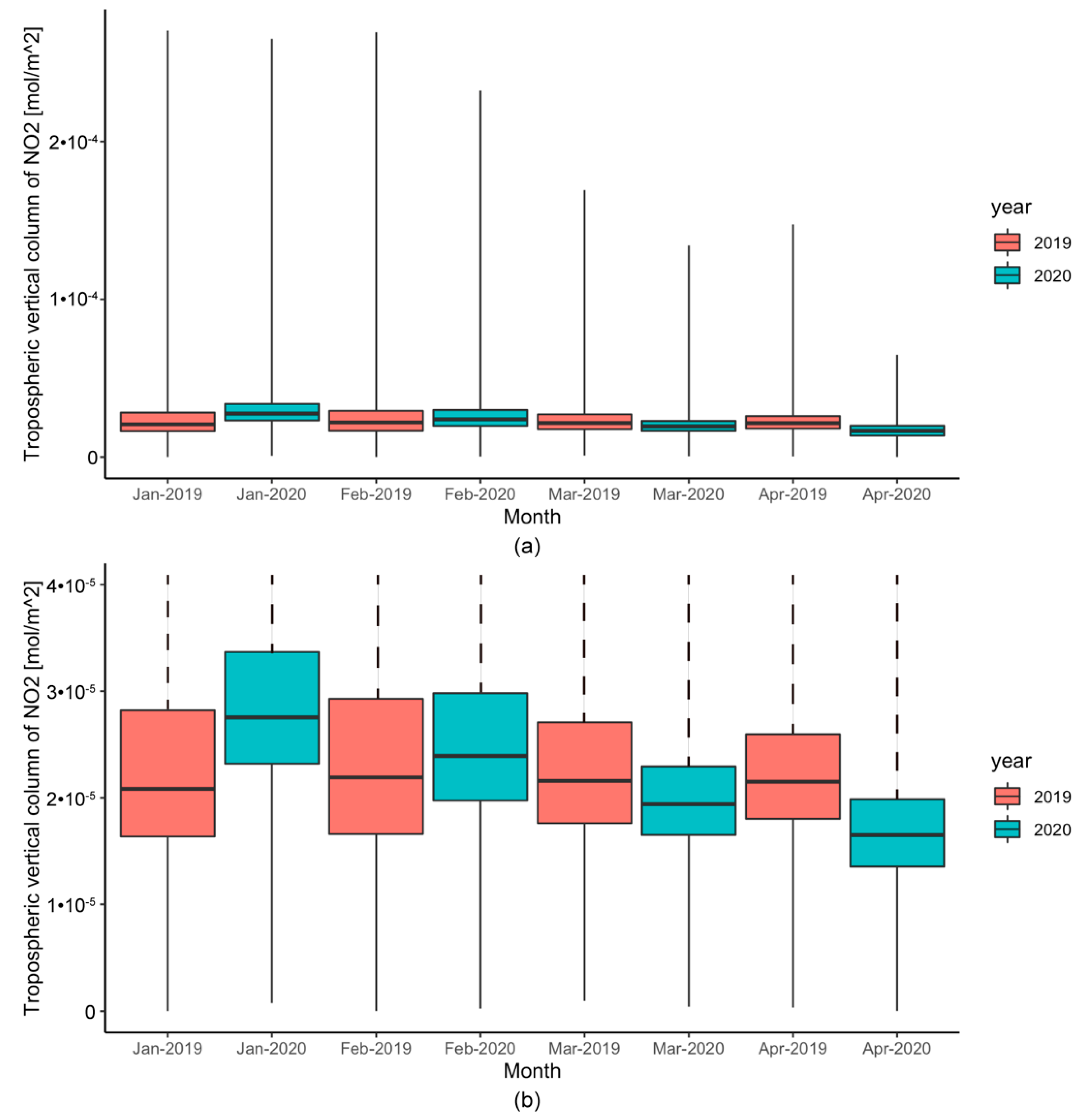
| Month | Year | Minimum | Maximum | Q25 | Median | Q75 |
|---|---|---|---|---|---|---|
| January | 2019 | 1.46 × 10⁻⁹ | 0.00027 | 1.64 × 10⁻⁵ | 2.08 × 10⁻⁵ | 2.82 × 10⁻⁵ |
| 2020 | 7.63 × 10⁻⁷ | 0.000265 | 2.32 × 10⁻⁵ | 2.75 × 10⁻⁵ | 3.37 × 10⁻⁵ | |
| February | 2019 | 7.41 × 10⁻⁹ | 0.000269 | 1.66 × 10⁻⁵ | 2.19 × 10⁻⁵ | 2.93 × 10⁻⁵ |
| 2020 | 2.4 × 10⁻⁷ | 0.000232 | 1.97 × 10⁻⁵ | 2.39 × 10⁻⁵ | 2.98 × 10⁻⁵ | |
| March | 2019 | 9.56 × 10⁻⁷ | 0.000169 | 1.76 × 10⁻⁵ | 2.16 × 10⁻⁵ | 2.71 × 10⁻⁵ |
| 2020 | 4.12 × 10⁻⁷ | 0.000134 | 1.65 × 10⁻⁵ | 1.94 × 10⁻⁵ | 2.29 × 10⁻⁵ | |
| April | 2019 | 3.32 × 10⁻⁷ | 0.000148 | 1.8 × 10⁻⁵ | 2.15 × 10⁻⁵ | 2.6 × 10⁻⁵ |
| 2020 | 1.25 × 10⁻⁸ | 6.49 × 10⁻⁸ | 1.35 × 10⁻⁵ | 1.65 × 10⁻⁵ | 1.99 × 10⁻⁵ |
© 2020 by the authors. Licensee MDPI, Basel, Switzerland. This article is an open access article distributed under the terms and conditions of the Creative Commons Attribution (CC BY) license (http://creativecommons.org/licenses/by/4.0/).
Share and Cite
Mesas-Carrascosa, F.-J.; Pérez Porras, F.; Triviño-Tarradas, P.; García-Ferrer, A.; Meroño-Larriva, J.E. Effect of Lockdown Measures on Atmospheric Nitrogen Dioxide during SARS-CoV-2 in Spain. Remote Sens. 2020, 12, 2210. https://0-doi-org.brum.beds.ac.uk/10.3390/rs12142210
Mesas-Carrascosa F-J, Pérez Porras F, Triviño-Tarradas P, García-Ferrer A, Meroño-Larriva JE. Effect of Lockdown Measures on Atmospheric Nitrogen Dioxide during SARS-CoV-2 in Spain. Remote Sensing. 2020; 12(14):2210. https://0-doi-org.brum.beds.ac.uk/10.3390/rs12142210
Chicago/Turabian StyleMesas-Carrascosa, Francisco-Javier, Fernando Pérez Porras, Paula Triviño-Tarradas, Alfonso García-Ferrer, and Jose Emilio Meroño-Larriva. 2020. "Effect of Lockdown Measures on Atmospheric Nitrogen Dioxide during SARS-CoV-2 in Spain" Remote Sensing 12, no. 14: 2210. https://0-doi-org.brum.beds.ac.uk/10.3390/rs12142210