Automated SAR Image Thresholds for Water Mask Production in Alberta’s Boreal Region


1
Resource Stewardship Division, Alberta Environment and Parks, 200 5 Avenue S, Lethbridge, AB T1J 4L1, Canada
2
Department of Geography, University of Lethbridge, 4401 University Drive W, Lethbridge, AB T1H 3M4, Canada
3
National Boreal Program, Ducks Unlimited Canada, 13370 78 Avenue, Surrey, BC V3W 0H6, Canada
4
Prairie Region, Ducks Unlimited Canada, 1030 Winnipeg Street, Regina, SK S4R 8P8, Canada
5
Canada Centre for Remote Sensing, Natural Resources Canada, 560 Rochester Street, Ottawa, ON K1S 5K2, Canada
*
Author to whom correspondence should be addressed.
Remote Sens. 2020, 12(14), 2223; https://0-doi-org.brum.beds.ac.uk/10.3390/rs12142223
Submission received: 26 May 2020
/
Revised: 29 June 2020
/
Accepted: 8 July 2020
/
Published: 11 July 2020
(This article belongs to the Special Issue Wetland Landscape Change Mapping Using Remote Sensing)
Abstract
:Mapping and monitoring surface water features is important for sustainably managing this critical natural resource that is in decline due to numerous natural and anthropogenic pressures. Satellite Synthetic Aperture Radar is a popular and inexpensive solution for such exercises over large scales through the application of thresholds to distinguish water from non-water. Despite improvements to threshold methods, threshold selection is traditionally manual, which introduces subjectivity and inconsistency over large scales. This study presents a novel method for objectively determining and applying a threshold to determine water masks from Synthetic Aperture Radar (SAR) imagery on a scene-by-scene basis. The method was applied to Radarsat-2 and simulated Radarsat Constellation Mission scenes, and validated against two independent validation sources with high accuracy (Kappa ranging from 0.85 to 0.93). Expectedly, greatest misclassification occurs near shorelines, which are often ecologically important zones. Comparisons between Radarsat-2 and Radarsat Constellation Mission thresholds and outputs suggest that the latter is a capable successor for surface water applications. This work represents a foundational step toward objectivity and consistency in large-scale water mapping and monitoring.
1. Introduction
1.1. Background
Understanding the location, extent, and abundance of terrestrial inland surface water features, including but not limited to open water wetlands, lakes, and rivers, contributes to understanding the hydrologic cycle, energy and biogeochemical cycles, aquatic habitats, and how to improve Earth system models [1,2]. In Canada, freshwater lakes and wetlands cover approximately 13% of the country’s land surface area [3]; however, these features represent a natural resource that is in decline due to natural and anthropogenic pressures. In the province of Alberta, approximately 66% of wetlands in settled parts of the province no longer exist because of climate warming, agricultural practices, and urban development [4]. The rates of wetland change in Alberta’s natural and crown land areas have not been accurately quantified [5], despite being subject to natural resource exploration and extraction pressures. As a result, there is need to identify and monitor Alberta’s surface water features in order to sustainably preserve this critical resource. This need is supported through Alberta’s Water Act [6] and other complementary policies and legislation (e.g., wetland policy) that aim to support and promote the conservation and management of water within the province.
Locating and identifying changes to terrestrial open water features is highly accurate via historically favoured “boots on the ground” approaches. However, these approaches are often spatially limited, very expensive, time consuming, and logistically challenging if the target locations are remote. As an alternative, remotely sensed aerial photographs have demonstrated success for manually delineating wetlands and surface water features with high accuracy [7,8]. This approach can be utilised at regional and theoretically national scales; however, interpretation requires analysts to possess knowledge of the mapping area and experience in the analysis of image tones [9]. Moreover, the acquisition of aerial data can be cost prohibitive whilst manual interpretation can be time consuming, and in regions of high variability (e.g., seasonal and/or inter-annual changes to water feature extent), field validation is still required [10].
Satellite remote sensing offers a large-scale solution for identifying surface water features [11,12]. Synthetic Aperture Radar (SAR) is an increasingly common data source for “water seeking” applications as it distinguishes water from land surfaces with high contrast. This is due to the high dielectric constant of a (smooth) water surface, making it a specular reflector, meaning very little backscatter is detectable at the sensor, causing it to appear dark in imagery [11,13]. While texture analysis (i.e., analysing the spatial variation in image appearance) has been used to threshold open water surfaces [14], the most common method of mapping these features is through backscatter intensity thresholding schemes [13,15,16], where backscatter below a defined threshold is classified as water. For example, DeLancey et al. [17] applied a threshold based on the local minimum between the land/water bimodal backscatter distribution. However, this approach assumes a distinct division in the backscatter distribution between water and land surfaces. Moreover, this approach may capture shoreline vegetation signatures, which may lead to their misclassification as water. An alternate method, developed by White et al. [18], which uses multiple noise filtering techniques, has been successfully applied across Canada and specifically in Alberta [19,20].
SAR data can be acquired with various polarisations. For example, Radarsat-2 transmits and receives either horizontally (H) or vertically (V) polarised electromagnetic waves in the following combinations: HH, HV, VH, and VV. Radarsat Constellation Mission simultaneously transmits horizontal and vertical waves to create circular (C) polarisation, and receives either horizontally or vertically polarised data. Each transmit–receive polarisation is stored in a unique “channel” where a single channel, two channels, or four channels are commonly stored depending on the sensor acquisition mode. Typically, HH data are optimal for mapping surface water features when little to no roughness is present across the water surface. Alternatively, HV demonstrates superior results for water surfaces with increased roughness because of high winds [21].
SAR has potential to become a valuable tool for water resource management and has the capacity for long-term surface water monitoring [22]. However, its greatest limitation is the often subjective selection of a suitable land/water threshold. The objective of this study is to mitigate this constraint by applying and assessing a novel method for automatically selecting an appropriate threshold for water mask development from SAR data. The study will apply the method to Radarsat-2 (RS-2) and simulated Radarsat Constellation Mission (RCM) data to demonstrate its efficacy for historic and future large-scale surface water mapping and monitoring.
1.2. Existing Threshold Methods
This study presents a novel method for objectively and automatically identifying surface water features from SAR imagery. This is an active area of research, and therefore, multiple methods for surface water detection using remote sensing exist. A brief summary of state-of-the-art surface water masks is provided, where the developed methods were applied to either optical [23,24,25] or SAR data [26,27].
Fang-fang et al. [23] used Landsat-5 and -7 imagery over five sites in China, investigating the ability of single-band thresholding and various spectral (vegetation and water) indices to map surface water features. The modified normalised difference water index (MNDWI) was determined as the best method for determining surface water features. However, it was concluded that a single “universal” water detection method was not applicable across all landscapes due to differences in topography and vegetation presence/density. Similarly, Tetteh and Schönert [25] utilised Rapideye optical imagery to detect and map surface water at a total of three sites in the USA, Brazil, and Mali. The NIR (near-infrared) band and four calculated indices were thresholded to create five intermediate water masks that were intersected to create a single intermediate water mask; morphological filtering was applied to derive the final water mask. Automatic threshold detection was determined over the NIR band through the analysis of its data distribution, whereas the threshold values for the spectral indices were fixed (based on analysis as a function of clear and muddy water and other terrestrial land cover classes). The Kappa statistics varied from 0.84 to 0.94 across the study sites. An acknowledged shortcoming of using optical data for water mask development is the presence of clouds and/or shadows in the imagery. This becomes challenging because surface water typically appears dark in imagery, similar to shadows cast by clouds and terrestrial objects (such as buildings, vegetation, etc.) that are adjacent to water features; dark road surfaces are also a common source of confusion [28].
Regarding SAR algorithms, Li and Wang [26] used single-polarised Radarsat-2 imagery to derive water masks for a prairie landscape in Manitoba, Canada. An adaptation of the Otsu thresholding method (which selects a threshold that maximises the between-class (water/non-water) variances of an image histogram) was employed to determine an objective threshold for surface water detection. A sub-imaging routine was employed to mitigate the uneven distribution of water and non-water classes that were present in the entire SAR scene, a preference of the Otsu method. Whilst this method proved accurate (Kappa ranging from 0.79 to 0.89), the sub-imaging routine does not always ensure that sub-images contain even distributions of water and non-water classes, which may lead to sub-optimal threshold selections.
A study from Pulvirenti et al. [29] employed COSMO-SkyMed SAR data in combination with a fuzzy logic classification approach over a study site near the city of Shkodër, Albania. The algorithm produced water extent maps that exhibited high agreement with other water extent estimates produced using SAR (TerraSAR-X, Radarsat) and optical (Formosat) imagery. Ground truth data were unavailable, therefore, clear accuracy metrics were also unavailable. The novelty of this method was its ability to identify not only open water surfaces but also flooded forested and agricultural areas. However, it is noted that mapping water extents by this approach is potentially time consuming. More recent work by Pulvirenti et al. [30] investigated the use of temporal trends of the SAR coherence (similarity between images) for assessing water extents in urban areas. However, it was noted that several factors may contribute to the decrease in the coherence in certain (urban) environments that are not influenced by flood or water extents.
A recent study by Hu et al. [27] utilised Sentinel-1 at a site in China, applying an innovative tiling selection method combined with the minimum error thresholding technique [31]. The tiling selection method initiates a round of selection and a subsequent refinement of the candidate tiles used for determining a water mask threshold based on backscatter intensity information. At the site level, high accuracy results were obtained, with Kappa ranging from 0.81 to 0.90, but as low as 0.58 at some site locations.
Airborne Light Detection and Ranging (LiDAR) data have also been utilised for surface water mapping techniques. Crasto et al. [32] mapped surface water in a deltaic environment using a decision tree applied strategically to selected LiDAR attributes such as intensity, scan angle, and point density. Moreover, the angle of intersection at which points were acquired was also a deterministic factor. Kappa statistics ranging from 0.91 to 0.98 were calculated across three transects of the acquired data, showcasing the potential of LiDAR for water mapping. Moreover, the employed methodology used an automatically selected threshold approach, avoiding the use of fixed thresholds, thus promoting methodological adaptability. However, high resolution airborne LiDAR is more computationally intensive to process than spaceborne optical and SAR data; moreover, aerial repeat acquisitions are costly and logistically impractical for most surface water monitoring applications, especially at large scales.
2. Study Site and Data
2.1. Utikuma Region Study Area
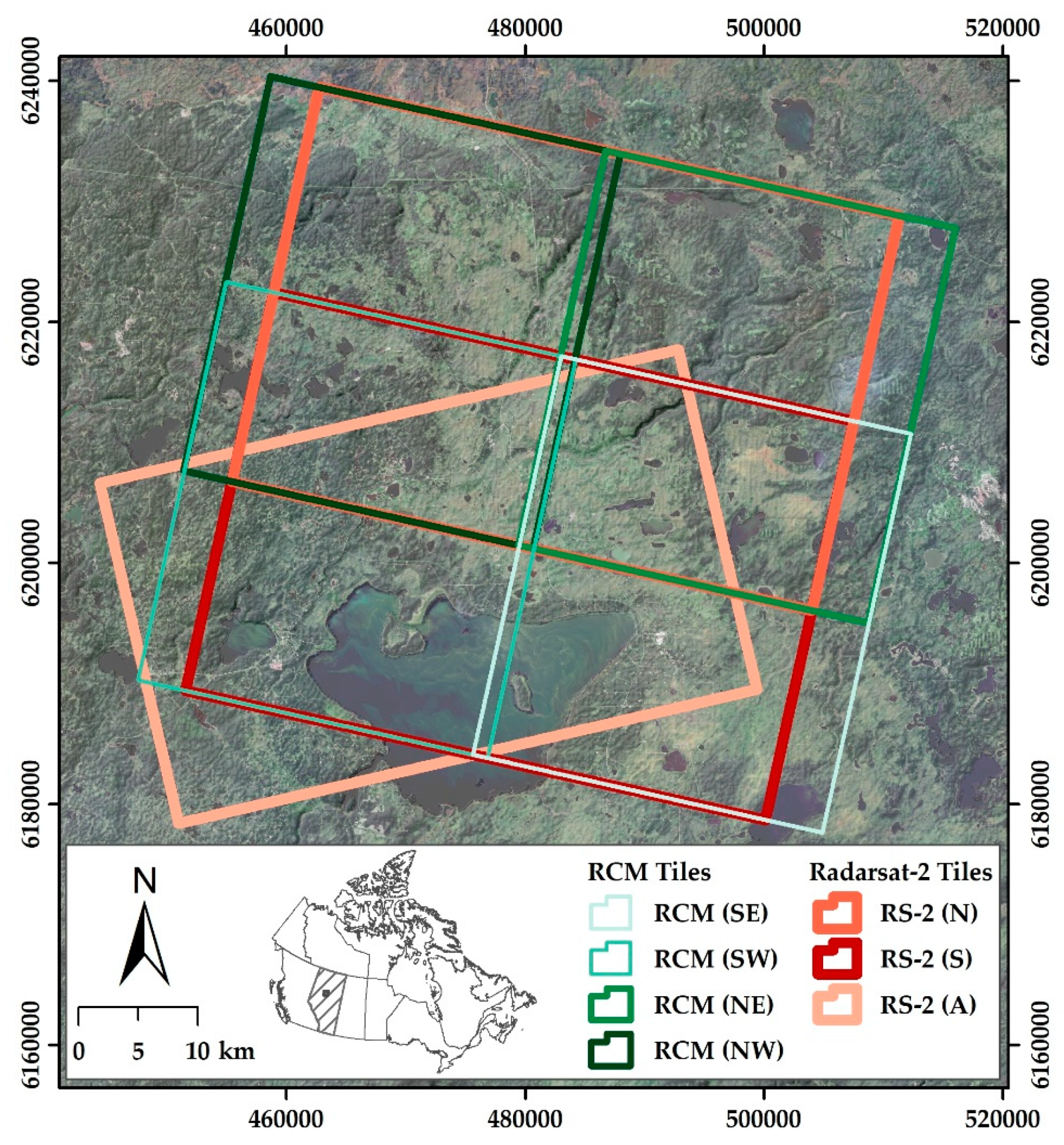
The Utikuma Region Study Area (URSA) is located within the central mixed-wood natural subregion of Alberta’s boreal forest [33], approximately 300 km northwest of Edmonton (Figure 1). The URSA was established to develop spatially explicit modelling tools for predicting the cumulative effects of natural and anthropogenic disturbances on Alberta’s Boreal Plains [34]. The URSA is characterized by moraine complexes that are comprised of a mixture of locally topographic low-lying areas of open water and flooded vegetation [34]. Ponds that can persist year-round range in area from ~0.4 ha up to and beyond 2000 ha, including Utikuma Lake, which constitutes a significant portion of the open water landscape at approximately 25,000 ha. The extent of this study is defined by a spatial composite of three overlapping Radarsat-2 quad-polarization images with an equivalent area of approximately 400,000 ha (Figure 1). Oil, gas, and forestry activities are active within the site boundary, where well pads, pipelines, seismic lines, and cut blocks characterise anthropogenic activity.
2.2. SAR Data
Two quad-polarised (HH, HV, VH, and VV) Wide Fine-Quad FQ10W beam mode RS-2 images were acquired on 27 July 2017 on a descending orbital pass (labelled RS-2 (N) and RS-2 (S); Figure 1). A single quad-polarised Wide Fine-Quad FQ5W image was acquired on 8 August 2017 on an ascending orbital pass (labelled RS-2 (A); Figure 1). These C-Band SAR images were acquired with near and far incidence angles ranging from 28.4° to 31.6° for descending orbits and from 22.5° to 26.0° for ascending orbits, respectively. The images were processed (prior to delivery) to single look complex (SLC) products that exhibited nominal near- and far-range resolutions of 10.9 m × 9.9 m (descending) and 13.6 m × 11.9 m (ascending), respectively.
Only RS-2 images acquired on a descending orbit (RS-2 (N) and RS-2 (S); Figure 1) were employed to simulate RCM images using the RCM-Sim 4.4 tool developed by Natural Resources Canada [35]. This tool approximates the planned form and structure of RCM data products, simulates RCM compact polarimetric (CP) data, creates RCM metadata, and mimics pseudo-ScanSAR SLC products based on pre-launch specifications provided by the Canadian Space Agency. For the current study, CP data were simulated at a nominal resolution of 16 m using the medium resolution 16M beam mode identifier. The CP configuration refers to Circular Transmit Linear Receive (CTLR), which was simulated as circular transmit (right-hand circular), horizontal (RH) and vertical (RV) receive in this study. The boundaries of the simulated RCM images extend beyond the perimeter of the study site by virtue of pre-launch RCM data delivery and structure definitions, which dictate that images are delivered with defined dimensions. As no RS-2 data were available for simulating RCM data in these external locations, they were defined as areas of no data and thus removed from the water mask analysis.
The SAR images were employed as candidate data to assess the proposed methodology for automatically determining appropriate thresholds for identifying surface water features on the landscape. These available data allowed for testing the consistency of the method between different sensors (RS-2 and RCM), across images acquired with different incidence angles (ascending versus descending), and in different beam modes from the same sensor (RS-2).
2.3. Validation Data
The Ducks Unlimited Canada developed Enhanced Wetland Classification (EWC) [36] and the Alberta Biological Monitoring Institute developed Advanced Landcover Prediction and Habitat Assessment (ALPHA) wetland inventory products were used to assess the accuracy of the derived water masks. The URSA EWC [37] is a 30 m resolution product developed using satellite remote sensing (Landsat) and manual editing, ensuring that the product is of high accuracy, and has been applied across much of the boreal region of Alberta. The EWC maps the areal coverage and extent of 19 distinct wetland classes, all of which can be transposed to align with surface water and non-water classes. The EWC at the study site was developed from multiple Landsat scenes, acquired in 1999 and 2002, yielding a product that exhibited a multi-year temporal disparity. However, this is not expected to have a significant effect on the surface water feature extents across the site as it is located in the Boreal Plains ecozone, which has high water availability for recharging basins [34]. In addition, the EWC raster exhibits some localised georeferencing errors originating from the orthorectification process. At the initiation of this EWC project, the underlying Landsat scene was outsourced to a commercial third party (Radarsat International) for orthorectification and topographic correction. This process was challenging due to a lack of accurate, high-resolution digital elevation models and ground control points [37]. Within the collection of ground control points used for orthorectification, some contained inherent errors due to photointerpretation difficulties associated with medium resolution imagery (i.e., 30 m). The resultant georeferenced Landsat scene therefore contains a range of error up to a maximum shift of two pixels (60 m) depending on location. This may affect the one-to-one statistical comparison between the mapped water products; however, this influence is expected to be minimal because the error is localised and not scene-wide. The EWC represents a comprehensive effort of combining remote sensing and manual editing to yield a highly accurate wetland inventory. No specific timeline exists for regular EWC updates; however, the commencement of the first update is expected by 2023.
The ALPHA wetland inventory [38] is classified into seven major classes (upland, bog, fen, swamp, marsh, open water, and wetland general) using a segmentation convolutional neural network (CNN) deep learning algorithm and trained using interpreted ABMI 3 × 7 km landcover photo-plots [39]. The product is derived using open-source Sentinel-1 (SAR) and Sentinel-2 (optical) remote sensing data available from the Google Earth Engine [40] and the Advanced Land Observation Satellite (ALOS) Digital Elevation Model (DEM). The product represents the most up-to-date (2019) large-scale boreal wetland inventory produced by ABMI, covering approximately 77% of Alberta, and is expected to be updated annually.
The ALPHA wetland inventory exhibits 1723 open water features available for the validation of derived water masks; by comparison, the EWC exhibits 1573 water features. This difference is expected as each product was developed using different methodological processes and from source imagery with different spatial resolutions (i.e., 30 m and 10 m, respectively).
3. Methods
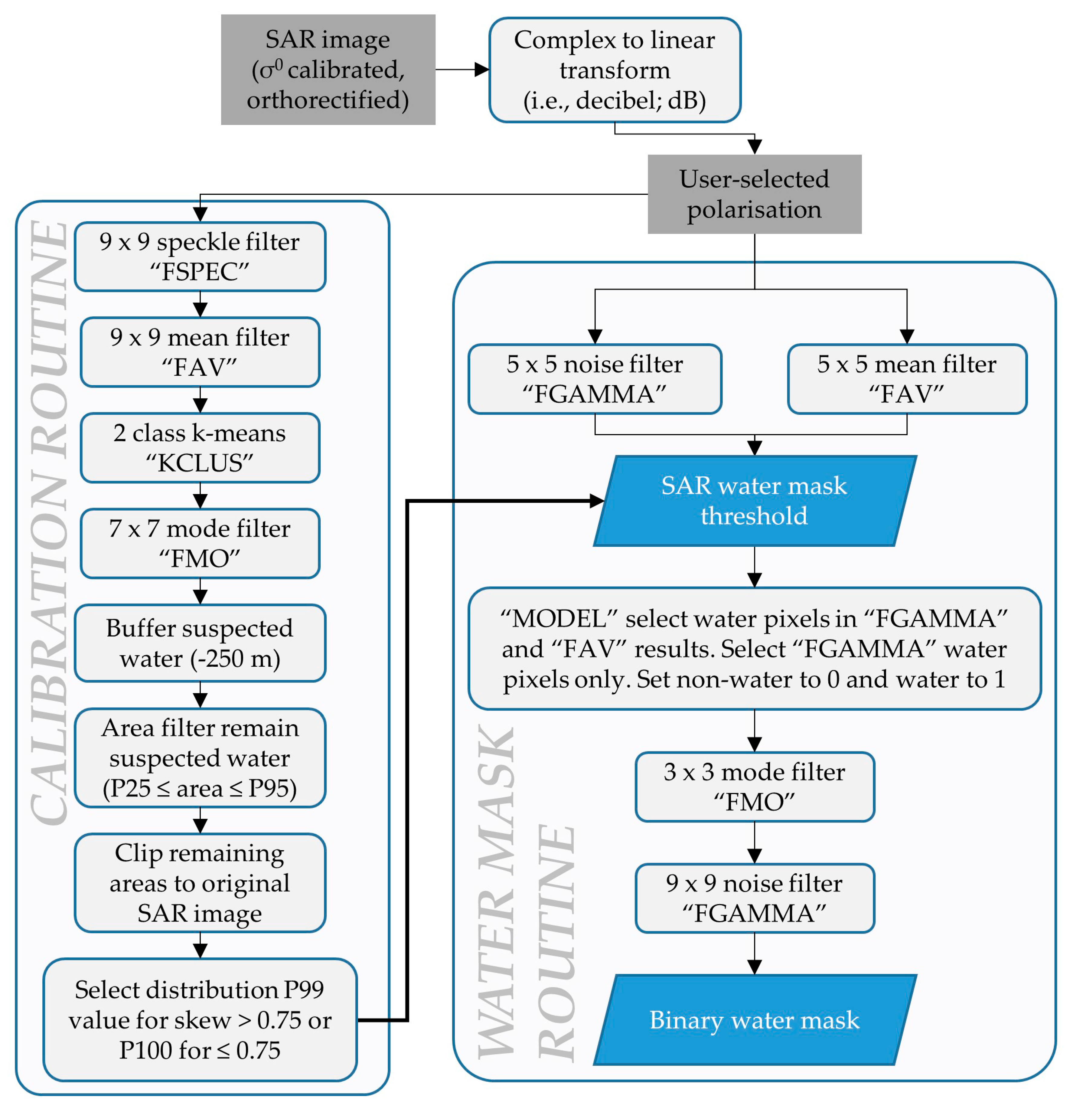
The methods for producing a binary water mask from SAR images are split into a pre-analysis step followed by two primary components: a calibration and water mask routine (Figure 2). In pre-analysis, SAR images should be orthorectified and calibrated to sigma-nought (σ0). Under the calibration routine, a single polarisation from the available SAR data is selected and analysed using the developed method to automatically determine a threshold for a water mask. Under the water mask routine, the threshold result from the calibration routine is utilised in a workflow to yield a binary water mask result.
3.1. Calibration Routine
The calibration routine for the automatic identification of SAR water mask thresholds was developed in the Python environment. The routine should be applied on a single radar channel (e.g., HH, HV, VH, or VV) image that is deemed most suitable given the landscape and acquisition time characteristics (e.g., HH for a smooth water surface or HV for a rough water surface). In this case, the selected image is converted to decibel units and calibrated to σ0. The routine follows multiple steps (Figure 2), each of which are performed using ESRI ArcMap and PCI Geomatica tools; however, some aspects of the routine may be applied using open-source software such as the Geospatial Data Abstraction Library (GDAL), Python, R, or Sentinel Toolbox. An example of spatial results from each step in the calibration routine are noted in Figure 3.
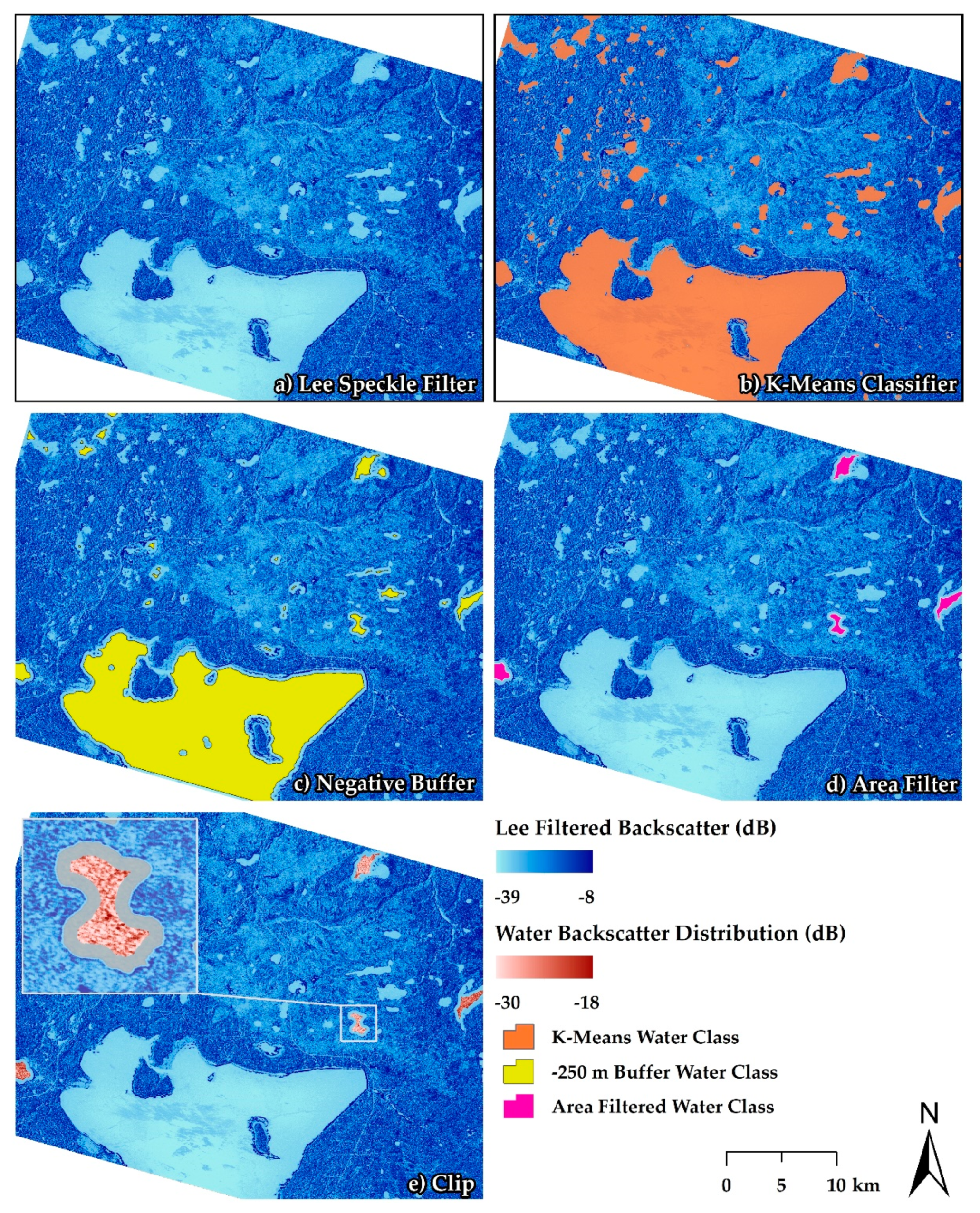
First, a 9 × 9 moving window Lee filter (FSPEC function in Geomatica) is applied to the selected SAR image, followed by a mean filter (FAV) of the same window dimensions. The window sizes were selected to be deliberately aggressive in cleaning speckle noise from the image and maximise the difference between the water and non-water surfaces (Figure 3a). An unsupervised k-means clustering classification (KCLUS) is applied to the result of the previous step, where a maximum of two output classes are permitted, and all other parameters are left as default (i.e., the maximum number of iterations and the convergence on the cluster position threshold were set to 20 and 0.01, respectively); for further details, see the PCI KCLUS manual [41]. Given that the greatest differences in the filtered backscatter image are expected between water and non-water features, the two output classes represent surface water (low backscatter) and non-water (high backscatter) classes (Figure 3b). A 7 × 7 window mode filter (FMO) is applied to the two-class output to reduce the number of small open water features captured by the unsupervised classifier. In post-filtering, the non-water class is removed from further analysis, and the water features are converted to polygons to accept GIS operations. Each polygon represents suspected areas of water; however, transition boundaries near shorelines may exhibit confusion with non-water. This is mitigated through the application of a negative buffer of 250 m (Figure 3c), which was deemed appropriate given the size of the open water features on the landscape. Small water features are removed as a consequence of buffer application if there is not >500 m of water between opposing shorelines. This is not expected to change the determined water mask threshold because the SAR backscatter from water is similar regardless of the feature size. The buffer size can be adjusted to suit the water feature size distribution. The remaining polygons were filtered by area in order to minimise the influence of small (<25th percentile; P25) and large (>95th percentile P95) features (Figure 3d). Small features may contain shoreline influences, whereas large features may be wind affected, which can artificially increase or decrease the backscatter values. The removal of these features allows for a more consistent representation of suspected water backscatter values across the image. The remaining features are used to clip the original SAR backscatter image to yield a distribution of values that are recorded from primarily water features (Figure 3e).
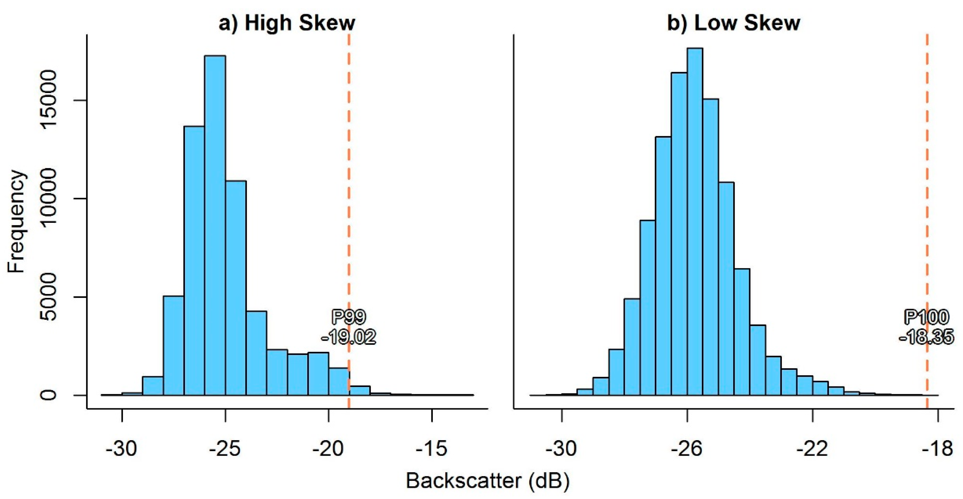
To determine the optimal SAR water mask threshold, the backscatter distributions are interrogated as a function of high (>0.75) positive skewness, which indicates the possible capture of vegetation signatures in the clipped backscatter values near shorelines. In order to mitigate the influence of possible vegetation signatures (which exhibit higher backscatter values than water), the 99th percentile (P99) value of the backscatter distribution is selected in order to remove extreme high values in the distribution (Figure 4a). Conversely, a low skew (≤0.75) distribution, which more closely resembles a normal distribution, is more indicative of scattering from a homogeneous surface. Therefore, the maximum (or 100th percentile; P100) of the backscatter distribution is selected as the SAR water mask threshold (Figure 4b).
3.2. SAR Water Mask Routine
The water mask routine spatially determines the areal extent of open water landscape features from SAR data and is performed following the method of White et al. [18] (although other threshold-based methods may be substituted as appropriate), which utilises a two-pronged approach (Figure 2). This method requires a threshold to be selected and applied to the SAR image where image values less than or equal to the threshold are assumed as open water. Here, the selected threshold is determined by the calibration routine rather than being manually selected as per the original method of White et al. [18]. The water mask routine is more sophisticated than simply applying a binary threshold across the entirety of the SAR image and considers multiple intermediate water masks to inform the final product. For further details on the water mask routine, see White et al. [18]. The water mask routine is executed in PCI Geomatica and applies a series of noise reduction filters, imposes the selected threshold, and applies additional noise reduction filters (Figure 2). The resultant water mask exhibits two classes: non-water (denoted as 0), and water (denoted as 1).
3.3. Water Mask Accuracy Assessment
The water mask accuracies were assessed against the EWC and the ALPHA wetland inventory products. Prior to assessment, both validation datasets were transposed to water and non-water classes. That is, for the EWC, the aquatic bed, open water, and mudflats classes were amalgamated as a single water class; all other classes were combined to a single non-water class. Similarly, the open water class from the ALPHA wetland inventory was used as the water reference, while all other classes were combined to a non-water class. Assessments were made using a variety of accuracy statistics calculated from a confusion matrix that is populated based on comparing all overlapping pixels between a reference/validation (EWC and ALPHA) and a simulation (RS-2 and RCM water masks) dataset. In this case, correctly identified water features (with respect to the reference data) are true positives, and incorrectly identified water features are false positives. Correctly identified non-water (terrestrial) features are true negatives, and incorrectly identified non-water features are false negatives. The accuracy statistics used for the water mask accuracy assessment include the sensitivity, specificity, balanced accuracy, F1-score, and Kappa (Table 1). Assessments were made for descending RS-2 and RCM simulated scenes only because the ascending RS-2 scene was captured during windy conditions and therefore necessitated that analysis be performed on the HV channel. As a result, the inclusion of this scene may confound the accuracy assessment results. Alternatively, overlapping areas between ascending and descending RS-2 scenes are compared for consistency (described below).
3.4. Overlap and Threshold Comparison
The overlapping areas between descending RS-2 scenes and simulated RCM scenes allows for comparisons between each of the derived water mask results. Comparisons between north and south RS-2 scenes, north–south RCM scenes in the west of the overlap area, and north–south RCM scenes in the east overlap area are summarised; the best suited RCM polarised imagery (i.e., that produced the most accurate water mask) was utilised for overlap comparisons. The arithmetic addition of the derived water mask (where zero values represent non-water and values of one are water) from each set of overlapping scenes allows for the identification of areas of agreement and disagreement; values of two indicate agreement, while values of one indicate disagreement. Water masks from RS-2 descending and ascending scenes were also compared to assess if the results differed significantly as a function of the incidence angle and/or different polarisation (HV for ascending scene in this case). Comparisons were made over the common area of overlap between the ascending and descending north scene, and the ascending and descending south scene.
The automatically determined thresholds and resulting accuracy statistics were compared between north, south, and ascending RS-2 scenes to identify differences in the respective water masks from each scene to provide insight into the stability of the threshold identified for each scene. A similar approach was executed for north and south RCM scenes where the RCM area of overlap was split into east and west areas (a consequence of the outputs from the RCM simulator). The overall accuracy and Kappa statistics were calculated for each water mask and compared in overlapping areas to indicate differences in the quality of the water masks as a function of each scene.
4. Results
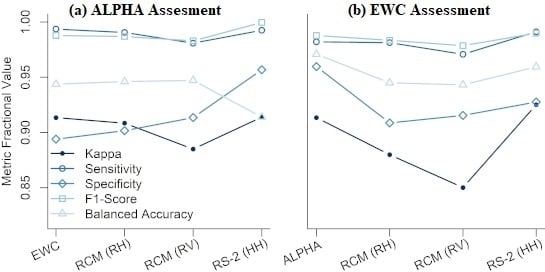
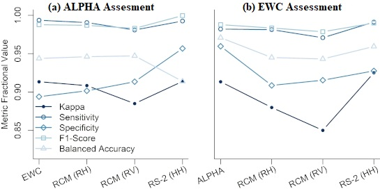
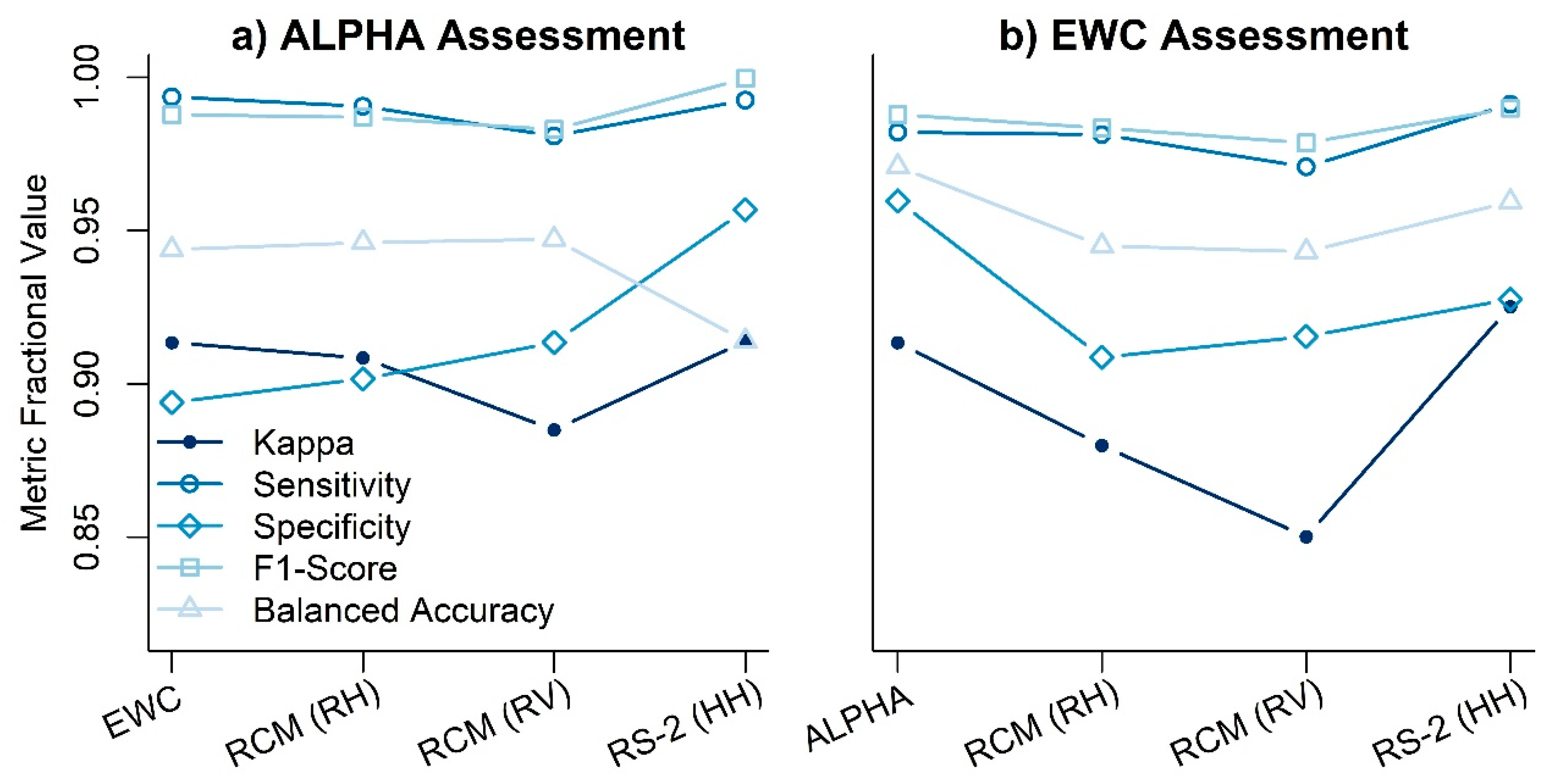
A suite of statistics (outlined in Table 1) were calculated to assess the accuracies of the water masks produced from RS-2 and simulated RCM data (Figure 5). All the generated water masks had accuracies exceeding 85%, and most were 95% or better. Water masks derived from RS-2 imagery yield greater accuracies than the RCM equivalents; this is true for both sources of validation data. Simulated RCM circular transmit-vertical receive (RV) polarised imagery consistently yields the lowest accuracy metrics, suggesting that RCM RH polarised imagery may be more suitable for deriving water masks. In general, accuracy metrics derived using the ALPHA wetland inventory are elevated compared to equivalents determined from the EWC.
Kappa is the most critical of the accuracy metrics when assessed using either the ALPHA wetland inventory or the EWC, except for the water mask derived from the RCM RH polarised imagery for ALPHA. Specificity is the second most critical accuracy metric in all cases with the exclusion of RCM (RH) (ALPHA assessment), where it is the most critical. Balanced accuracy is third most critical of the accuracy metrics, followed by F1-score and sensitivity, where the latter metrics indicate potential bias, producing near-perfect (i.e., a value of 1) results.
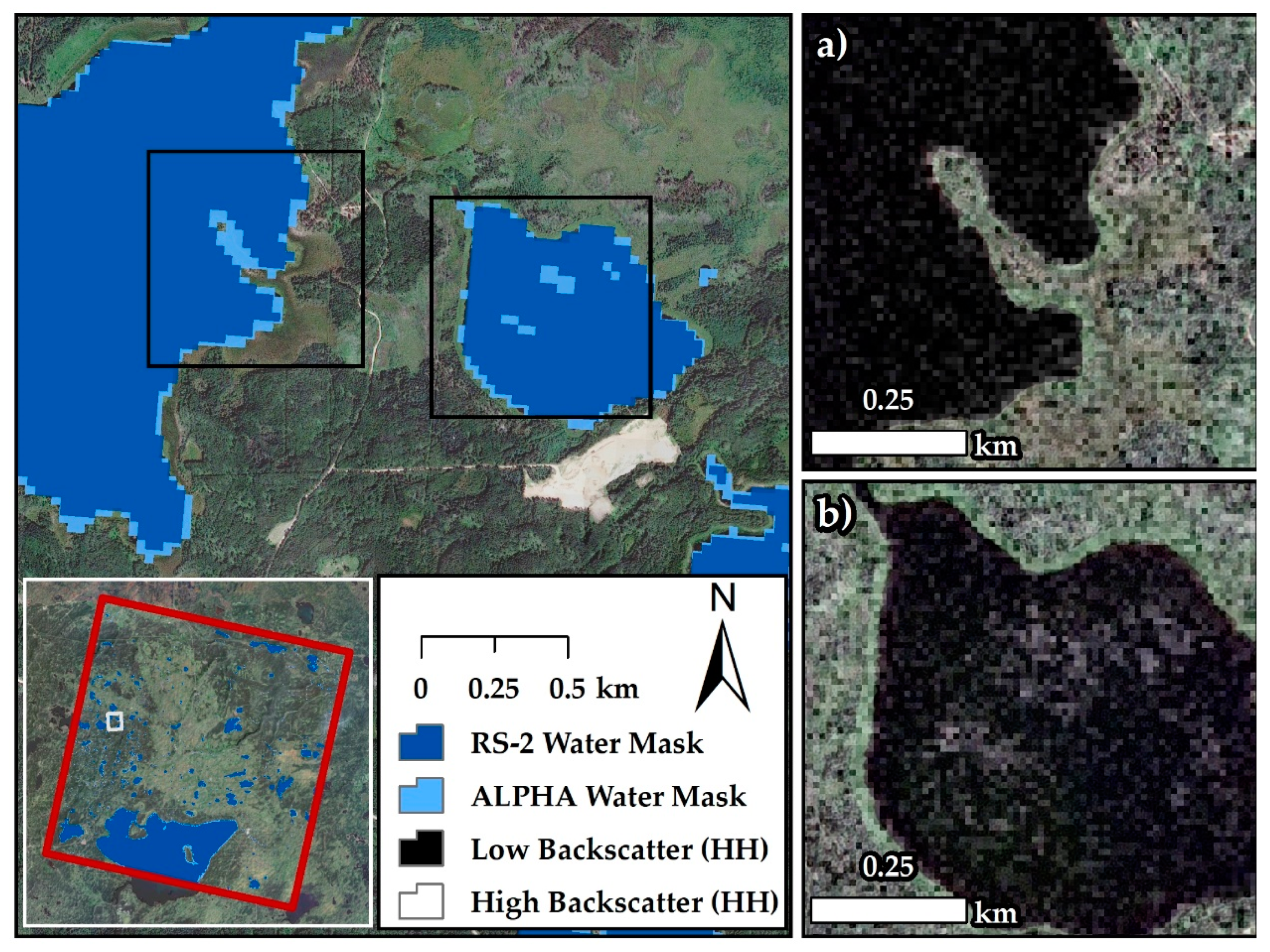
The calculated accuracy statistics provide a summary over the entire classification area but do not offer a detailed accuracy assessment at boundary and/or transition locations, where misclassification rates are expected to be greatest. This is illustrated in Figure 6 where the ALPHA wetland inventory is compared to the RS-2 water mask. In the left box, the ALPHA wetland inventory suggests that no peninsula of land protrudes into the lake, whereas the opposite is noted in the RS-2 water mask, resulting in elevated false negatives. Similarly, in the right box, the RS-2 water mask produced false negatives where island features were perceived but are absent in the ALPHA dataset. The number of false negatives is minor at small scales and appears negligible when compared to the number of pixels that represent an entire waterbody (as in Figure 6). However, over regional scales (and beyond), such differences can lead to significant discrepancies in surface water extent.
Overlap Comparison
Areas overlapping between a subset of RS-2 and RCM scenes were utilised to compare differences in automatically determined thresholds and resulting water mask accuracies as a function of the sensor scene (i.e., same sensor) and between sensors. The results suggest that the thresholds were broadly consistent between overlapping scenes of RS-2, where the greatest differences were noted between overlapping ascending and descending scenes (Table 2). Conversely, little difference was noted between north–south (descending) scenes, and greater differences were noted between overlapping (north–south) RCM scenes derived from descending RS-2, where the greatest magnitude difference was noted in the east (Table 2). Despite the relatively large inter-scene differences between thresholds, the accuracy statistics suggest high correspondence between the eastern north and south RCM scenes, whereas lower correspondence is observed between the western overlap despite greater similarity in thresholds. Similarly, little difference is noted for overlapping ascending and descending RS-2 scenes for overall accuracy and Kappa, where the latter highlights small variability between scenes; however, the magnitude of the differences falls within the range of the differences noted in Kappa for RCM. It is noted that any variability present within the threshold and accuracy metrics for the ascending RS-2 scene may be a result of different incidence angles, beam modes, analysed polarisation channels, or a combination of each. Little difference is observed between overlapping RS-2 descending scenes as indicated by the highest overall accuracy and Kappa statistics amongst all overlapping scenes.
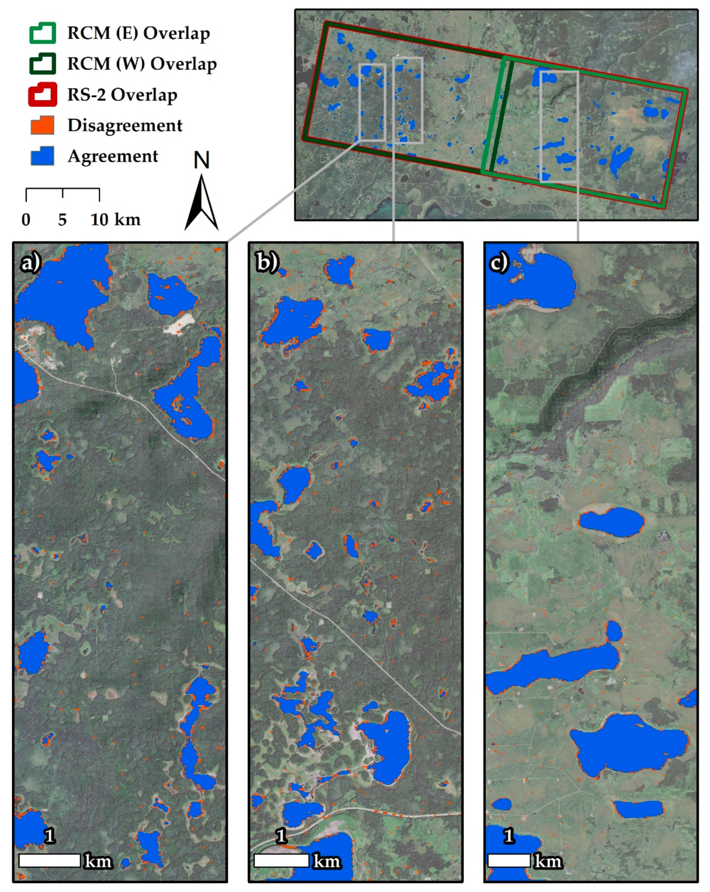
The variability in the accuracy statistics between overlapping scenes is corroborated as a function of the areal extent of disagreement (i.e., areas that are water in one of the overlapping scenes but non-water in the other) (Figure 7). The majority of disagreement is observed around shorelines and in isolated pixels, the majority of which are most evident in the comparison of west RCM scenes.
5. Discussion
5.1. Water Mask Assessment
The RS-2 water masks were more accurate than the RCM equivalents, a result largely expected due to the −32 dB noise floor of RS-2 compared to −25 dB for the simulated RCM products. Of the calculated accuracy metrics (Figure 5), Kappa was least favourable, suggesting that for the data examined in this study, it offers the least biased, most balanced accuracy measure over a binary classification. The F1-score, which is typically used to yield accuracy information on a per class basis, where the number of classes is greater than two, appears to be biased and unsuitable for assessing the accuracy of binary classifications. As a measure of the true positive rate, the sensitivity is biased if few false negatives are classified (i.e., water is incorrectly classified as non-water), which appears to be the case in this study; however, this does not determine sensitivity to be unsuitable for assessing the accuracies of such a classification. Comparing the high sensitivity and the reduction in specificity suggests that non-water was incorrectly classified as water at a rate greater than that at which water was incorrectly classified as non-water (Figure 6).
The resultant automatically determined thresholds provided water masks that were broadly consistent between overlapping images. In addition, comparisons between overlapping RS-2 and RCM scenes demonstrate little variability in the accuracy metrics, suggesting that the threshold method objectively selects a suitable threshold to yield consistent results. This is further exemplified in the comparison between ascending and descending RS-2 scenes, where the threshold values exhibit a mean difference of 5 dB; despite this, the overall accuracy and Kappa statistics remain broadly consistent. However, the source of variability between ascending and descending is confounded by multiple factors, including different incidence angles, different beam modes, and the necessitated use of the HV channel due to the high winds at the time of data acquisition.
The water masks derived from RS-2 and simulated RCM scenes where assessed using a suite of accuracy metrics and compared over the EWC and ALPHA wetland inventory. Both datasets were employed for validation as they represent the only large-scale, fit-for-purpose datasets available. In general, the accuracy metrics derived between the ALPHA wetland inventory and the EWC are reduced compared to those for the best-performing SAR water mask (RS-2). This suggests that the spatial offset between the EWC (resulting from orthorectification difficulties) and the other water masks are not insignificant. This highlights that differences can exist between “validated” products that are broadly accepted.
5.2. Method Comparison Challenges
It is challenging to assess if one automatic threshold method is better than another or if other methods are superior to that presented because different methods were used to obtain a water mask via the application of the automatically determined threshold. The presented method makes use of the water mask method of White et al. [18], whereas the methods developed by Li and Wang [26] and Hu et al. [27] (representing a small cross-section of literature) utilise entropy, texture, and/or contour refinement techniques to assist in surface water detection. In addition, each study was performed at different locations, resulting in the presence of inherent variability as a function of specific site characteristics. Although it is challenging to gauge the performance of each automatic thresholding method, the presented methodology is amongst the most simple and generally applicable methods for any SAR data source.
5.3. Surface Water Mapping and Monitoring
Repeat data acquisitions over the same location multiple times are common with SAR sensors, making them ideal for monitoring surface water features over time. Moreover, Canada’s investment in SAR technology (evident through the Radarsat-1, Radarsat-2, and Constellation Mission programs) makes it possible for legacy monitoring back to 1996 using Radarsat-1 and -2 sensors. Coupled with recent (and future) acquisitions from RCM, there is potential to provide a surface water time series that spans up to 30 years, provided that RCM meets its expected lifespan. Additional SAR sensors—such as the National Aeronautics and Space Administration Indian Space Research Organisation SAR (NISAR) mission, due for launch in 2021—can further compliment monitoring activities. Of interest, the advantage of RCM and NISAR over previous SAR missions is their greater swath sizes, thus potentially making them more operationally viable because mission mapping extents will be less restricted [35].
RCM’s nominal repeat pass period of 4 days coupled with its ability to identify surface water makes it ideal for monitoring surface water intra- and inter-annually. RCM RH polarised imagery appears to be more suitable for water mask derivation where data are acquired under calm conditions. However, this may not be the case for data acquired where the water surface exhibits increased roughness. The most suitable imagery for water mask derivation from RCM’s predecessors, Radarsat-1 and -2, varied as a function of water surface roughness. Typically, HH polarised imagery produced the most accurate water masks when acquired under calm conditions, whereas HV imagery yielded superior results under windy conditions. Additional investigation is required to determine if an alternative polarisation is better suited to surface water identification where data are acquired under turbulent conditions for RCM.
The comparison of overlapping water masks suggests that RCM may not be as internally consistent as RS-2, as evident in the derived accuracy statistics and observed areal extent of disagreement between overlapping scenes (Table 2, Figure 7). Of interest, western overlapping scenes exhibit the greatest disagreement, which may be related to the increased forest cover and, therefore, perceived surface roughness, which is a known influencer of SAR backscatter mechanisms. This theory is corroborated through the reduced forest cover presence in the eastern area of overlap; however, further investigation is required to provide confirmation. Moreover, it is important to note that simulated RCM data may differ from the actual RCM data, which may lead to slightly different results.
The short- and long-term monitoring of surface water has implications for water policy and land use activities, and provides critical information that enables decision makers to implement strategic legislation to safeguard the longevity of fresh surface water as a resource.
5.4. Automatic Threshold Application to Alternate SAR Sensors
The developed automatic threshold method was deliberately designed to be universally applicable to any orthorectified SAR image sourced from any SAR sensor. This is realised using simple GIS tools that can be applied to appropriately post-processed SAR imagery (i.e., converted to decibels and appropriately calibrated). The results from other SAR sensors will vary as a function of the image resolution, polarisation, and potential calibration (where the latter points are noted in accuracy metric differences between RS-2 and RCM). The developed routine has only been applied to σ0 calibrated images. Whilst application to SAR images with alternate calibrations (e.g., β0 and γ0) is not expected to be problematic, additional investigation may be warranted to determine if different calibrations induce variable threshold identifications.
The application of the developed objective calibration routine to multiple sensors is beneficial on numerous fronts, two of which are that (1) a long archive of data can be accessed to create a long time series of surface water features for monitoring and change detection, and (2) validation can be performed against multiple data sources, informing of any changes via multiple evidence streams. Moreover, the use of an automatic and objective methodology applied to multiple SAR data sources minimises the need for manual intervention (other than QAQC) and enables program management with few personnel and/or financial resources. Such methods are ideal for adaptation to integrate with cloud-based monitoring programs.
5.5. Application to Rivers
Previous investigations that used SAR to map river and canal channels in Europe have demonstrated a range of accuracies (Kappa from 0.47 to 0.74) depending on the use of single- or dual-polarised imagery, where the latter consistently yielded superior results [44]. However, the methods investigated still produce gaps in river networks (i.e., areas where water was present but not detected), even with high-resolution SAR imagery (e.g., 3 m resolution). The mapping of small river/canal channels with the proposed method may be challenging, especially with the SAR imagery employed in this study, due to the resolution at which the image data were acquired, particularly as image manipulation (via applied filters) may further confound pure surface water features. This is unlikely to be resolved by application to future SAR sensors, such as RCM, as the image resolutions will be comparable to those of current sensors. However, current and future SAR sensors are capable of acquiring data at finer, more appropriate resolutions for river and stream mapping (e.g., using spot light modes, acquiring data at a 3 m resolution for RS-2 and RCM). However, these image modes typically require “tasking” to an acquisition area, can be cost prohibitive, and can be computationally intensive to analyse over large scales. The upcoming Surface Water and Ocean Topography (SWOT) mission is mandated to map rivers ≥ 100 m wide according to the SWOT mission statement. However, the proposed 50 m image resolution to be employed over inland surface water bodies (including rivers) is unlikely to map narrow rivers accurately, leaving narrow river network connectivity issues unaddressed. An alternate means of determining riverine open water areas may be realised using fine resolution (typically no larger than 1 m; [45]) optical imagery such as that obtained from Worldview, aerial photos, or drones [46].
5.6. Accuracy Assessment Bias
As demonstrated in this study, typical land cover accuracy assessment metrics can be limited in their ability to express the true accuracy of binary classifications (such as water masks). This is because of the large number of pixels that constitute water body centres versus the relatively small number of pixels that constitute the shoreline. The centres of water bodies are easier to classify because they appear homogeneous in imagery; by contrast, classifying shorelines is challenging because of increased heterogeneity through the presence of mixed water and non-water pixels. This is further confounded when analysing image time series, as the shoreline expands and contracts seasonally. Furthermore, in the current study, the presence of Utikuma Lake, in the south of the study site, skews the accuracy metrics. In the derived RS-2 water mask, Utikuma Lake constitutes approximately 68% of the total water surface area within the study site. As a result, correctly classifying the majority of Utikuma Lake would yield an overall accuracy of approximately 68%, whereas correctly classifying all the other surface water features would yield an overall accuracy of only 32%.
These compounding effects suggest that innovative accuracy assessment methods are required to provide a more robust assessment of water masks (and other land cover classifications). One solution may be achieved through the use of multiple accuracy metrics beyond the typical suite of overall, user’s, and producer’s accuracies. The results suggest that the inclusion of Cohen’s Kappa and specificity offer additional insight into potential misclassification, as these metrics appear to be the most sensitive to such misclassification. However, the method used for the accuracy assessment influences the resulting accuracy metrics and therefore should be adapted to minimise bias towards large features with more constituent pixels.
In consideration of minimising bias in accuracy metrics, an alternate method for assessing accuracy metrics may utilise an object-based approach. That is, each collection of adjacent pixels with the same predicted classification is summarised by a single value that represents the object as a whole. This method enforces that large and small objects have equal weight in accuracy metric calculations, as objects with more pixels within their perimeter are still represented by a single classification value, identical to all other objects. Alternatively, the ratio of shoreline to non-shoreline pixels may be a useful statistic for use in the calculation of accuracy metrics to negate the bias that larger classified features have on their outcome. These methods are not fully developed, and their advantages and disadvantages are yet to be comprehensively assessed. Additional work is required to fully develop and assess such methods for their ability to represent the accuracy of land cover classifications.
6. Conclusions
This study presented a novel method for automatically and objectively determining a threshold for deriving water masks from RS-2 and RCM imagery. The presented method utilised simple GIS and image backscatter distribution analysis to determine an objective threshold that was applied through a proven water mask method. Key results demonstrate (i) that the developed SAR water mask threshold method produced high accuracy water masks (compared to two independent datasets); (ii) that RCM shows potential for accurately (average Kappa = 0.91) mapping and monitoring surface water features, despite lower accuracies compared to RS-2 (average Kappa = 0.95) (largely attributed to RCM’s higher noise floor); (iii) that despite small differences, high agreement between RS-2 (ascending and descending) and RCM water masks demonstrates that the presented method is robust and consistent.
The novelty of the presented calibration routine is its general applicability to all SAR datasets using the physical terrain and in situ water features as a way of objectively determining a SAR image threshold. A key advantage is that a user requires no experience with mapping or delineating water extents, and the water mask routine (based on White et al. [18] here) can be substituted as appropriate. The method provides an efficient prototypical approach to operationally mapping and monitoring surface water, allowing for the past and future assessment of state of the environment reporting and resource monitoring. This is a valuable tool for effectively and strategically managing surface water resources across the globe.
Future Work
A suite of accuracy statistics used to assess water mask accuracy revealed potential bias in binary land cover classifications, evident from consistently favourable values. As a result, it is suggested that future work should concentrate on the development of robust unbiased accuracy assessment methods; the suggested methods may distinguish shoreline and non-shoreline pixels. In addition, evaluating the calibration routine over a Prairie pothole landscape is the next logical step to test its efficacy for delineating small surface water features within the province of Alberta. Beyond Alberta, future work should compare this routine with other state-of-the-art methods employing the same datasets (RS-2 and RCM). Additionally, investigations should apply the current routine to other SAR sensors with X-, S-, L-, and P-bands and over other challenging coastal environments.
Author Contributions
Conceptualisation, C.M.; methodology, C.M.; software, C.M.; validation, C.M.; formal analysis, C.M.; data curation, M.M., C.H., and B.B.; writing—original draft preparation, C.M. and M.M.; writing—review and editing, C.M., M.M., L.B., C.H., and B.B.; visualisation, C.M..; supervision, C.M., M.M., L.B., and C.H.; project administration, L.B. and C.H.; funding acquisition, C.M., C.H., and L.B. All authors have read and agreed to the published version of the manuscript.
Funding
This research was funded through Ducks Unlimited Canada, the Mitacs Elevate program (grant number IT08294) and Alberta Innovates – Energy & Environment Solutions (grant number E323726).
Acknowledgments
The authors wish to thank François Charbonneau for access to and assistance in executing the Radarsat Constellation Mission simulator. The Advanced Landcover Prediction and Habitat Assessment (ALPHA) products are available for download from the Alberta Biodiversity and Monitoring Institute (https://www.abmi.ca/home/data-analytics/da-top/da-product-overview/Advanced-Landcover-Prediction-and-Habitat-Assessment--ALPHA--Products.html). The Enhanced Wetland Classification data were provided by Ducks Unlimited Canada.
Conflicts of Interest
The authors declare no conflict of interest.
References
- Kyzivat, E.D.; Smith, L.C.; Pitcher, L.H.; Fayne, J.V.; Cooley, S.W.; Cooper, M.G.; Topp, S.N.; Langhorst, T.; Harlan, M.E.; Horvat, C.; et al. A High-Resolution Airborne Color-Infrared Camera Water Mask for the NASA ABoVE Campaign. Remote Sens. 2019, 11, 2163. [Google Scholar] [CrossRef] [Green Version]
- National Academies of Sciences, Engineering, and Medicine. National Academies of Sciences—Engineering and Medicine. In Thriving on Our Changing Planet: A Decadal Strategy for Earth Observation from Space; The National Academies Press: Washington, DC, USA, 2018; p. 716. [Google Scholar] [CrossRef]
- Environment and Climate Change Canada. Canadian Environmental Sustainability Indicators: Extent of Canada‘s Wetlands. Available online: https://www.canada.ca/en/environment-climate-change/services/environmental-indicators/extent-wetlands.html (accessed on 30 November 2019).
- Government of Alberta. Alberta Wetland Policy. 2013. Available online: https://open.alberta.ca/publications/9781460112878 (accessed on 30 November 2019).
- Chasmer, L.; Hopkinson, C.; Montgomery, J.; Petrone, R. A Physically Based Terrain Morphology and Vegetation Structural Classification for Wetlands of the Boreal Plains, Alberta, Canada. Can. J. Remote Sens. 2016, 42, 521–540. [Google Scholar] [CrossRef]
- Government of Alberta. Water Act. Revised Statutes of Alberta 2000, Chapter W-3; Alberta Queen‘s Printer: Edmonton, AB, Canada, 2017. [Google Scholar]
- Szantoi, Z.; Escobedo, F.; Abd-Elrahman, A.; Smith, S.; Pearlstine, L. Analyzing fine-scale wetland composition using high resolution imagery and texture features. Int. J. Appl. Earth Obs. Geoinf. 2013, 23, 204–212. [Google Scholar] [CrossRef]
- Cowardin, L.M.; Carter, V.; Golet, F.C.; LaRoe, E.T. Classification of Wetlands and Deepwater Habitats of the United States US; Department of the Interior Fish and Wildlife Service: Washington, DC, USA, 1979.
- Anderson, R.R.; Wobber, F.J. Wetlands Mapping in New Jersey. Photogramm. Eng. Remote Sens. 1973, 47, 223–227. [Google Scholar]
- Cowardin, L.M.; Gilmer, D.S.; Mechlin, L.M. Characteristics of central North Dakota wetlands determined from sample aerial photographs and ground study. Wildl. Soc. Bull. 1981, 9, 280–288. [Google Scholar]
- Irwin, K.; Beaulne, D.; Braun, A.; Fotopoulos, G. Fusion of SAR, Optical Imagery and Airborne LiDAR for Surface Water Detection. Remote Sens. 2017, 9, 890. [Google Scholar] [CrossRef] [Green Version]
- Merchant, M.A.; Warren, R.K.; Edwards, R.; Kenyon, J.K. An Object-Based Assessment of Multi-Wavelength SAR, Optical Imagery and Topographical Datasets for Operational Wetland Mapping in Boreal Yukon, Canada. Can. J. Remote Sens. 2019, 45, 308–332. [Google Scholar] [CrossRef]
- White, L.; Brisco, B.; Dabboor, M.; Schmitt, A.; Pratt, A. A Collection of SAR Methodologies for Monitoring Wetlands. Remote Sens. 2015, 7, 7615–7645. [Google Scholar] [CrossRef] [Green Version]
- Peiman, R.; Ali, H.; Brisco, B.; Hopkinson, C. Performance evaluation of SAR texture algorithms for surface water body extraction through an open source python-based engine. In Proceedings of the 2017 IEEE International Geoscience and Remote Sensing Symposium (IGARSS), Fort Worth, TX, USA, 23–28 July 2017; pp. 3125–3127. [Google Scholar]
- Brisco, B.; Shelat, Y.; Murnaghan, K.; Montgomery, J.; Fuss, C.; Olthof, I.; Hopkinson, C.; Deschamps, A.; Poncos, V. Evaluation of C-Band SAR for Identification of Flooded Vegetation in Emergency Response Products. Can. J. Remote Sens. 2019, 45, 73–87. [Google Scholar] [CrossRef]
- Gstaiger, V.; Huth, J.; Gebhardt, S.; Wehrmann, T.; Kuenzer, C. Multi-sensoral and automated derivation of inundated areas using TerraSAR-X and ENVISAT ASAR data. Int. J. Remote Sens. 2012, 33, 7291–7304. [Google Scholar] [CrossRef]
- DeLancey, E.R.; Brisco, B.; Canisius, F.; Murnaghan, K.; Beaudette, L.; Kariyeva, J. The Synergistic Use of RADARSAT-2 Ascending and Descending Images to Improve Surface Water Detection Accuracy in Alberta, Canada. Can. J. Remote Sens. 2019, 45, 759–769. [Google Scholar] [CrossRef]
- White, L.; Brisco, B.; Pregitzer, M.; Tedford, B.; Boychuk, L. RADARSAT-2 Beam Mode Selection for Surface Water and Flooded Vegetation Mapping. Can. J. Remote Sens. 2014, 40, 135–151. [Google Scholar] [CrossRef]
- Montgomery, J.; Brisco, B.; Chasmer, L.; Devito, K.; Cobbaert, D.; Hopkinson, C. SAR and Lidar Temporal Data Fusion Approaches to Boreal Wetland Ecosystem Monitoring. Remote Sens. 2019, 11, 161. [Google Scholar] [CrossRef] [Green Version]
- Montgomery, J.S.; Hopkinson, C.; Brisco, B.; Patterson, S.; Rood, S.B. Wetland hydroperiod classification in the western prairies using multitemporal synthetic aperture radar. Hydrol. Process. 2018, 32, 1476–1490. [Google Scholar] [CrossRef]
- Brisco, B. Mapping and Monitoring Surface Water and Wetlands with Synthetic Aperture Radar. In Remote Sensing of Wetlands: Applications and Advances; Tiner, W.R., Lang, M.W., Klemas, V.V., Eds.; CRC Press: Boca Raton, FL, USA, 2015; pp. 119–136. [Google Scholar]
- Vickers, H.; Malnes, E.; Høgda, K.-A. Long-Term Water Surface Area Monitoring and Derived Water Level Using Synthetic Aperture Radar (SAR) at Altevatn, a Medium-Sized Arctic Lake. Remote Sens. 2019, 11, 2780. [Google Scholar] [CrossRef] [Green Version]
- Fang-fang, Z.; Bing, Z.; Jun-sheng, L.; Qian, S.; Yuanfeng, W.; Yang, S. Comparative Analysis of Automatic Water Identification Method Based on Multispectral Remote Sensing. Procedia Environ. Sci. 2011, 11, 1482–1487. [Google Scholar] [CrossRef] [Green Version]
- Vinayaraj, P.; Oishi, Y.; Nakamura, R. Development of an Automatic Dynamic Global Water Mask Using Landsat-8 Images. In Proceedings of the IGARSS 2018—2018 IEEE International Geoscience and Remote Sensing Symposium, Valencia, Spain, 22–27 July 2018; pp. 822–825. [Google Scholar]
- Tetteh, G.O.; Schönert, M. Automatic Generation of Water Masks from RapidEye Images. J. Geosci. Environ. Prot. 2015, 3, 7. [Google Scholar] [CrossRef]
- Li, J.; Wang, S. An automatic method for mapping inland surface waterbodies with Radarsat-2 imagery. Int. J. Remote Sens. 2015, 36, 1367–1384. [Google Scholar] [CrossRef]
- Hu, S.; Qin, J.; Ren, J.; Zhao, H.; Ren, J.; Hong, H. Automatic Extraction of Water Inundation Areas Using Sentinel-1 Data for Large Plain Areas. Remote Sens. 2020, 12, 243. [Google Scholar] [CrossRef] [Green Version]
- Bochow, M.; Heim, B.; Küster, T.; Rogaß, C.; Bartsch, I.; Segl, K.; Reigber, S.; Kaufmann, H. On the Use of Airborne Imaging Spectroscopy Data for the Automatic Detection and Delineation of Surface Water Bodies. In Remote Sensing of Planet Earth; Chemin, Y., Ed.; InTech: Rijeka, Croatia, 2012; p. 22. [Google Scholar]
- Pulvirenti, L.; Pierdicca, N.; Chini, M.; Guerriero, L. An algorithm for operational flood mapping from Synthetic Aperture Radar (SAR) data based on the fuzzy logic. Nat. Hazard Earth Syst. Sci. 2011, 11, 529–540. [Google Scholar] [CrossRef] [Green Version]
- Pulvirenti, L.; Chini, M.; Pierdicca, N.; Boni, G. Flood Detection in Urban Areas: Analysis of Time Series of Coherence Data in Stable Scatterers. In Proceedings of the IGARSS 2019—2019 IEEE International Geoscience and Remote Sensing Symposium, Yokohama, Japan, 28 July–2 August 2019; pp. 9745–9747. [Google Scholar]
- Kittler, J.; Illingworth, J. Minimum error thresholding. Pattern Recognit. 1986, 19, 41–47. [Google Scholar] [CrossRef]
- Crasto, N.; Hopkinson, C.; Forbes, D.L.; Lesack, L.; Marsh, P.; Spooner, I.; van der Sanden, J.J. A LiDAR-based decision-tree classification of open water surfaces in an Arctic delta. Remote Sens. Environ. 2015, 164, 90–102. [Google Scholar] [CrossRef]
- Natural Regions Committee; Downing, D.J.; Pettepiece, W.W. Natural Regions and Subregions of Alberta; Publication Number T/852; Government of Alberta: Edmonton, AB, Canada, 2006.
- Devito, K.J.; Mendoza, C.; Petrone, R.M.; Kettridge, N.; Waddington, J.M. Utikuma Region Study Area (URSA)—Part 1: Hydrogeological and ecohydrological studies (HEAD). For. Chron. 2016, 92, 57–61. [Google Scholar] [CrossRef] [Green Version]
- Charbonneau, F.J.; Brisco, B.; Raney, R.K.; McNairn, H.; Liu, C.; Vachon, P.W.; Shang, J.; DeAbreu, R.; Champagne, C.; Merzouki, A.; et al. Compact polarimetry overview and applications assessment. Can. J. Remote Sens. 2010, 36, S298–S315. [Google Scholar] [CrossRef]
- Smith, K.; Smith, C.; Forest, S.; Richard, A. A Field Guide to the Wetlands of the Boreal Plains Ecozone of Canada; Western Boreal Office: Edmonton, AB, Canada, 2007; p. 98. [Google Scholar]
- Ducks Unlimited. A User’s Guide to the Enhanced Wetland Classification for the Al-Pac Boreal Conservation Project; Ducks Unlimited Inc.: Rancho Cordova, CA, USA, 2008; p. 67. [Google Scholar]
- ABMI. Predictive Landcover (PLC) 3.0 and ABMI Wetland Inventory—Metadata; ABMI: Edmonton, AB, Canada, 2019. [Google Scholar]
- ABMI. ABMI 3×7 Photoplot Land Cover Dataset Data Model; ABMI: Edmonton, AB, Canada, 2016. [Google Scholar]
- Gorelick, N.; Hancher, M.; Dixon, M.; Ilyushchenko, S.; Thau, D.; Moore, R. Google Earth Engine: Planetary-scale geospatial analysis for everyone. Remote Sens. Environ. 2017, 202, 18–27. [Google Scholar] [CrossRef]
- PCI Geomatics. K-Means Clustering. Available online: https://www.pcigeomatics.com/geomatica-help/references/pciFunction_r/python/P_kclus.html (accessed on 30 June 2020).
- Derczynski, L. Complementarity, F-score, and NLP Evaluation. In Proceedings of the Tenth International Conference on Language Resources and Evaluation (LREC′16), Portorož, Slovenia, 23–28 May 2016; pp. 261–266. [Google Scholar]
- Cohen, J. A Coefficient of Agreement for Nominal Scales. Educ. Psychol. Meas. 1960, 20, 37–46. [Google Scholar] [CrossRef]
- Klemenjak, S.; Waske, B.; Valero, S.; Chanussot, J. Automatic Detection of Rivers in High-Resolution SAR Data. IEEE J. Sel. Top. Appl. Earth Obs. Remote Sens. 2012, 5, 1364–1372. [Google Scholar] [CrossRef] [Green Version]
- Marcus, W.A.; Fonstad, M.A. Optical remote mapping of rivers at sub-meter resolutions and watershed extents. Earth Surf. Process. Landforms 2008, 33, 4–24. [Google Scholar] [CrossRef]
- Kasvi, E.; Salmela, J.; Lotsari, E.; Kumpula, T.; Lane, S.N. Comparison of remote sensing based approaches for mapping bathymetry of shallow, clear water rivers. Geomorphology 2019, 333, 180–197. [Google Scholar] [CrossRef]
Figure 1.
Study site location within Alberta, Canada. The spatial extents of the employed Synthetic Aperture Radar (SAR) images are illustrated by colours: descending orbit acquired Radarsat-2 (RS-2) north (N) and south (S) images, an ascending orbit acquired image (RS-2 (A)), and simulated (from Radarsat-2 images) Radarsat Constellation Mission (RCM) southeast (SE), southwest (SW), northeast (NE), and northwest (NW) images (for descending RS-2 images only).

Figure 2.
Schematic workflow for determining an objective Synthetic Aperture Radar (SAR) water mask threshold (calibration routine) for use in the derivation of a binary water mask from SAR imagery (water mask routine), adapted from White et al. [18]. SAR data are processed through a series of ArcMap and PCI Geomatica functions, noted in quotation marks.

Figure 3.
Visualisation of the SAR water mask threshold calibration routine. (a) The SAR backscatter image is subject to a Lee speckle filter, followed by (b) a 2-class K-Means unsupervised classification. (c) A negative buffer (−250 m) is applied to remove transitional shoreline influences, (d) the resultant polygons from which are filtered by area to remove potential wind and/or aquatic vegetation effects. (e) The remaining polygons are used to clip the original SAR backscatter image to yield a surface water backscatter distribution.

Figure 4.
Comparison of threshold selection as a function of (a) high and (b) low skew backscatter distributions.
Figure 4.
Comparison of threshold selection as a function of (a) high and (b) low skew backscatter distributions.

Figure 5.
Illustration of multiple statistics for assessing the accuracies of the Radarsat-2 (RS-2) and Radarsat Constellation Mission (RCM) water masks derived using the developed automatic threshold selection routine. Each water mask was assessed against (a) the Advanced Landcover Prediction and Habitat Assessment (ALPHA) Wetland Inventory product and (b) the Ducks Unlimited Canada Enhanced Wetland Classification (EWC). Letters in parentheses refer to the SAR polarisation used for water mask derivation, where RH refers to right-hand circular transmit and horizontal receive, RV is the same as the later but vertical receive, and HH is horizontal transmit and receive.

Figure 6.
Visual comparison of the most accurate derived water mask from Radarsat-2 data and the Advanced Landcover Prediction and Habitat Assessment (ALPHA) wetland inventory product. Product agreement decreases near shorelines, (a) peninsulas, and (b) small islands (as perceived by the higher Radarsat-2 backscatter).

Figure 7.
Comparison of water masks for (a) overlapping north and south Radarsat-2 (RS-2) scenes, (b) north–south (west) simulated Radarsat Constellation Mission (RCM) scenes, and (c) north–south (east) RCM scenes.
Figure 7.
Comparison of water masks for (a) overlapping north and south Radarsat-2 (RS-2) scenes, (b) north–south (west) simulated Radarsat Constellation Mission (RCM) scenes, and (c) north–south (east) RCM scenes.


Table 1.
Summary of metrics used to assess the accuracies of the water masks derived using the automated threshold selection methodology.
Table 1.
Summary of metrics used to assess the accuracies of the water masks derived using the automated threshold selection methodology.
| Accuracy Metric | Description |
|---|---|
| Sensitivity (Se) | The true positive rate, or the number of correctly identified water features compared with correctly identified water features and incorrectly non-water features. |
| Specificity (Sp) | The true negative rate, or the number of correctly identified non-water features compared to the correctly identified non-water features and incorrectly identified water features. |
| Balanced Accuracy | Mean of the sensitivity and specificity. Provides a balanced accuracy assessment based on incorrectly identified water and non-water features. |
| F1-score | Useful for unbalanced validation data. F1-score is the harmonic average of precision (i.e., the ratio of correct positive predictions to the total predicted positives) and sensitivity (ranging from 0 to 1). See Derczynski [42] for further details. |
| Kappa | Measure of agreement between the reference and simulated data. Kappa ranges from −1 to 1, and values greater than 0 indicate agreement greater than that expected by chance; values below 0 indicate agreement worse than that expected by chance. See Cohen [43] for details. |
Table 2.
Summary and comparison of automatically derived thresholds for Radarsat-2 (RS-2) and Radarsat Constellation Mission (RCM) scenes for areas of overlap. Note, N-S corresponds to north–south overlap, where N-S (E) relates to east areas of north–south overlap, and N-S (W) similarly relates to west areas. A-N corresponds to ascending and north RS-2 scene overlap, and A-S similarly corresponds to ascending-south overlap. The differences between scene thresholds are calculated as noted in overlap (e.g., N-S denotes the south image threshold being subtracted from the north image threshold).
| Threshold | |||||||
|---|---|---|---|---|---|---|---|
| Data | Overlap | Overall Accuracy | Kappa | North | South | Ascending | Difference |
| RCM (RH) | N-S (E) | 0.99 | 0.93 | −22.47 | −23.39 | - | 0.92 |
| N-S (W) | 0.98 | 0.87 | −22.74 | −21.98 | - | −0.76 | |
| RS-2 | N-S | 0.99 | 0.98 | −19.02 | −18.35 | - | −0.67 |
| A *-N | 0.99 | 0.94 | −19.02 | - | −23.77 | 4.75 | |
| A *-S | 0.99 | 0.92 | - | −18.35 | −23.77 | 5.42 |
* Water mask for ascending image derived from HV polarisation; all other RS-2 water masks derived from HH.
© 2020 by the authors. Licensee MDPI, Basel, Switzerland. This article is an open access article distributed under the terms and conditions of the Creative Commons Attribution (CC BY) license (http://creativecommons.org/licenses/by/4.0/).
Share and Cite
MDPI and ACS Style
Mahoney, C.; Merchant, M.; Boychuk, L.; Hopkinson, C.; Brisco, B. Automated SAR Image Thresholds for Water Mask Production in Alberta’s Boreal Region. Remote Sens. 2020, 12, 2223. https://0-doi-org.brum.beds.ac.uk/10.3390/rs12142223
AMA Style
Mahoney C, Merchant M, Boychuk L, Hopkinson C, Brisco B. Automated SAR Image Thresholds for Water Mask Production in Alberta’s Boreal Region. Remote Sensing. 2020; 12(14):2223. https://0-doi-org.brum.beds.ac.uk/10.3390/rs12142223
Chicago/Turabian StyleMahoney, Craig, Michael Merchant, Lyle Boychuk, Chris Hopkinson, and Brian Brisco. 2020. "Automated SAR Image Thresholds for Water Mask Production in Alberta’s Boreal Region" Remote Sensing 12, no. 14: 2223. https://0-doi-org.brum.beds.ac.uk/10.3390/rs12142223
Note that from the first issue of 2016, this journal uses article numbers instead of page numbers. See further details here.