Detection of Very Small Tree Plantations and Tree-Level Characterization Using Open-Access Remote-Sensing Databases

Abstract

Highly fragmented land property hinders the planning and management of single species tree plantations. In such situations, acquiring information about the available resources is challenging. This study aims to propose a method to locate and characterize tree plantations in these cases. Galicia (Northwest of Spain) is an area where property is extremely divided into small parcels. European chestnut (Castanea sativa) plantations are an important source of income there; however, it is often difficult to obtain information about them due to their small size and scattered distribution. Therefore, we selected a Galician region with a high presence of chestnut plantations as a case study area in order to locate and characterize small plantations using open-access data. First, we detected the location of chestnut plantations applying a supervised classification for a combination of: Sentinel-2 images and the open-access low-density Light Detection and Ranging (LiDAR) point clouds, obtained from the untapped open-access LiDAR Spanish national database. Three classification algorithms were used: Random Forest (RF), Support Vector Machine (SVM), and XGBoost. We later characterized the plots at the tree-level using the LiDAR point-cloud. We detected individual trees and obtained their height applying a local maxima algorithm to a point-cloud-derived Canopy Height Model (CHM). We also calculated the crown surface of each tree by applying a method based on two-dimensional (2D) tree shape reconstruction and canopy segmentation to a projection of the LiDAR point cloud. Chestnut plantations were detected with an overall accuracy of 81.5%. Individual trees were identified with a detection rate of 96%. The coefficient of determination R² value for tree height estimation was 0.83, while for the crown surface calculation it was 0.74. The accuracy achieved with these open-access databases makes the proposed procedure suitable for acquiring knowledge about the location and state of chestnut plantations as well as for monitoring their evolution.

1. Introduction

Forestry policies rely strongly on the available knowledge about forest resources [1]. Investing in effective forest assessment and monitoring would help to reduce data gaps and, consequently, to support policy-making processes [2], such as the design of financial incentives and management of sector trade-offs [3]. At the European scale, one of the objectives of the Ministerial Conference on the Protection of Forests in Europe [4] is to update the tools for sustainable monitoring and assessing of forestry. The objective is to support sustainable forest management at the regional, national, or European levels by compiling knowledge about the quantity and quality of the goods and services that are produced and used [5,6].

One issue that forestry policy must deal with is fragmented rural ownership. This is one of the most significant obstacles for profitable rural management on a global scale [7,8,9]. Fragmented rural ownership is a very common phenomenon in developed countries [10], and it is gradually increasing due to the dissociation between forestry and small-scale farming, and to the limited involvement of landowners in forest management [11]. Small plots account for a large share of forestland. In 2010, Hirsch and Schmithüsen [12] reported that 61% of all European private forest holdings were less than one hectare.

Crucial information about forest plots and dynamics can be efficiently retrieved through remote sensing techniques [13,14,15]. When the focus is the mapping of forest cover, passive satellite sensors are the most-commonly used due to their high radiometric resolution [16,17]. However, the spatial resolution of multispectral sensors from freely-available satellite imagery reaches 15 m in Landsat-8—only in the panchromatic spectral band—[18] and 10 m in four spectral bands from Sentinel-2 [19]. When land cover is very fragmented these sensors provide images where several land cover classes might be present over the geographic area that correspond to a single pixel, resulting in pixels with mixed radiometry. Although advanced classification methods are available (machine learning, subpixel analysis, library-based, etc.), remote-sensing-based detection of pure forest patches of less than one hectare remains poorly studied. The reviews on remote sensing applied to forest inventories by White et al. [20] and Gómez et al. [21], for instance, refer to areas of at least 120 ha and 1000 ha, respectively. The satellite sensors with fine spatial resolution (Pléiades-1, 2 m, World View-4, 1.2 m) could be an alternative to analyze fragmented landscapes. Conrad et al. [22] performed a crop classification on fields with areas of a minimum size of 0.05 ha using the 6.5 m-resolution imagery of RapidEye. To map smallholders farming (ranging typically from 0.1 to 0.5 ha), Crespin-Boucaud et al. [23] used one very high spatial resolution image from the Satellite Pour l’Observation de la Terre (SPOT) 6 satellite, along with open-access data provided by Sentinel-2 and Landsat-8. The main limitation in using of high spatial resolution satellite sensors for large areas lies in their high acquisition costs, which can range from $12.5 Km² to $22.5 Km², or even higher depending on the provider, the type of product, and the level of processing, amongst other factors [24].

In order to be better able to detect small parcels, the information from different sensors and platforms has been evaluated [25,26]. Airborne Light Detection and Ranging (LiDAR) is the sensor that is most-commonly used to capture the structural attributes of a forest stand [27]. LiDAR systems send laser pulses toward the ground and measure the return time for reflections off vegetation surfaces and the ground [28]. This measured time, together with the coordinates of the lighted point provided by a geopositioning system, allow a LiDAR system to generate a three-dimensional (3D)-point cloud of the scanned surface. Laser pulses can penetrate the canopy permitting the 3D imaging of the vertical strata of the vegetation. The study by Xu et al. [29], which focuses on data provided by the 5 m-spatial resolution imagery of RapidEye and by aircraft-LiDAR in radiata pine stands, stands out in the field of LiDAR-based detection of very small, forested areas. A different approach was followed by Palenichka et al. [30], who developed an algorithm for multi-scale segmentation of forested areas, from a stand level to an individual-tree level. Their source of information was airborne LiDAR data.

LiDAR is also used to estimate structural parameters: tree position, height, canopy shape, and species identification [31,32]. Aircraft-LiDAR is often used in the statistical area-based approach (ABA) [33], where forest attributes of an area of interest are inferred through the combination of field measurements and canopy LiDAR point clouds [34]. When forest inventories require estimates of structural attributes at stand or sub-stand levels (0.5–50 ha) with relative errors below 10%, ABA-LiDAR methods are inadequate due to the need for data at tree level [21]. LiDAR acquired from Unmanned Aerial Vehicles (UAVs) can be used in these cases, since it yields a denser point cloud, which greatly facilitates the application of the individual tree detection (ITD) approach [35]. However, LiDAR data is usually acquired ad hoc in the study area [36,37,38].

A data source that can support the managing of small plots at a regional or national scale is the National LiDAR databases, which are available for an entire national territory. In the case of Spain, this database is LiDAR-Plan Nacional de Ortofotografía Aérea (PNOA) [39]. Although it was released in 2008 and is updated every 4–5 years, is it still under-exploited in forestry. In fact, in Scopus when ‘PNOA’, ‘LiDAR’, and ‘forestry’ are searched in the title, abstract and keywords, only a single document is listed. This kind of data source allows us to completely avoid fieldwork to acquire LiDAR data. Research on the potential of this low-resolution LiDAR data in the characterization of individual trees remains scarce, especially in agroforestry. Nowadays low-resolution LiDAR point clouds are available for the entire national territory of several countries. There is an increasing demand for research and exploitation of these data [21,40]. There is evidence of their potential in the field of agroforestry. For instance, Novero et al. [41] were able to classify land into four crops in the frame of the Phil-LiDAR program of the Philippines, with a point cloud density of 2 points/m². With regard to ad hoc LiDAR data acquisition, Parent et al. [36] developed an automated algorithm for land cover mapping using low density airborne LiDAR (1.56 points/m²) and high resolution multispectral imagery. Mohan et al. [37] detected individual trees in coconut plantations using a LiDAR point cloud of 5 points/m². Kathuria et al. [38] executed individual tree detection as well by using LiDAR with a mean point density of 2 points/m².

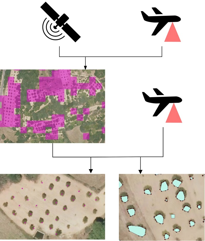
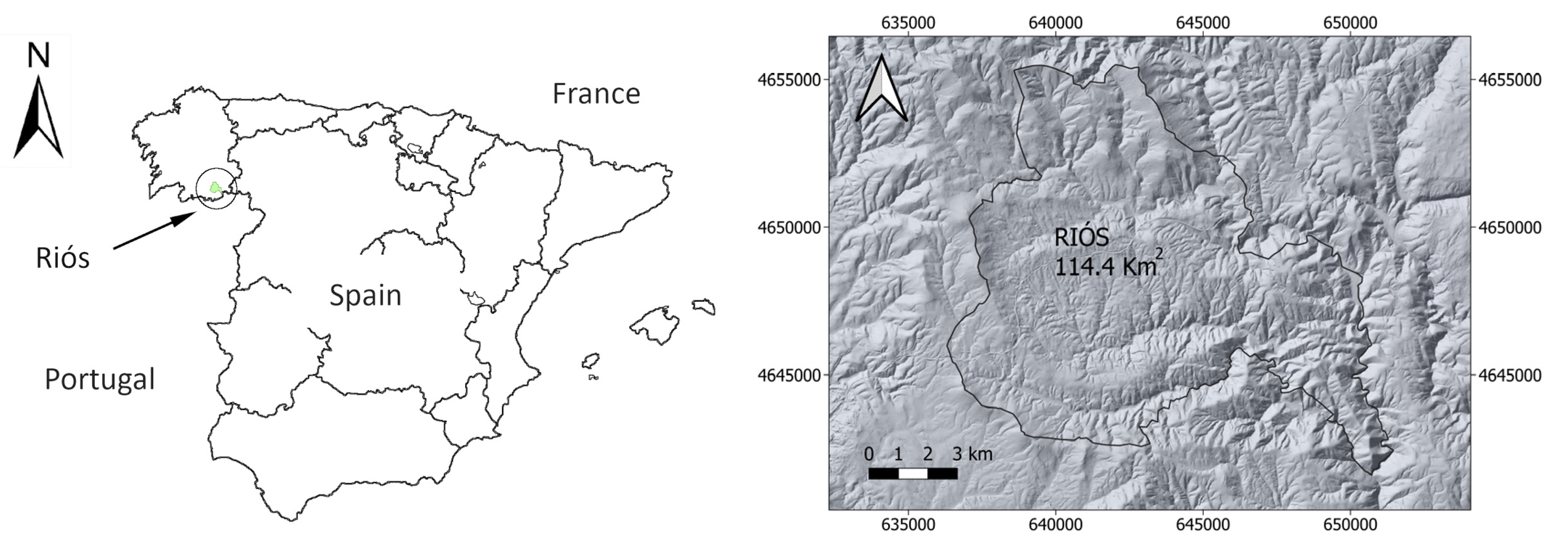
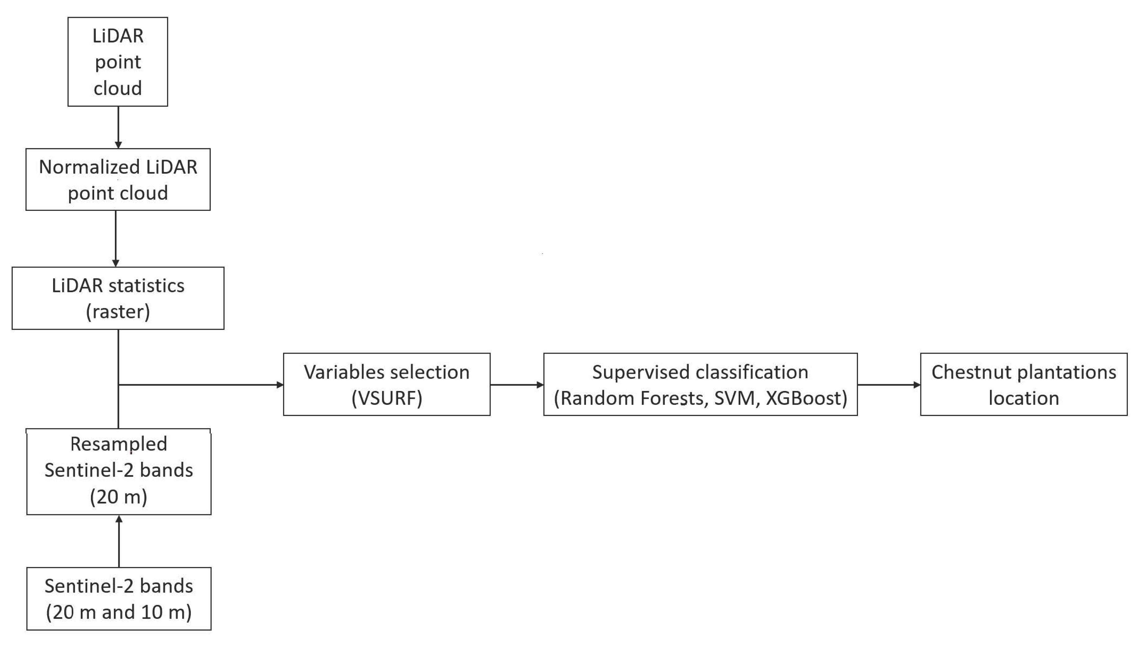
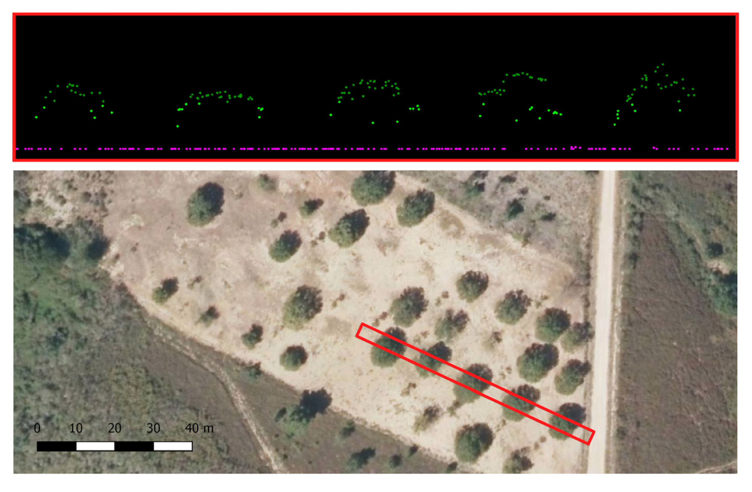
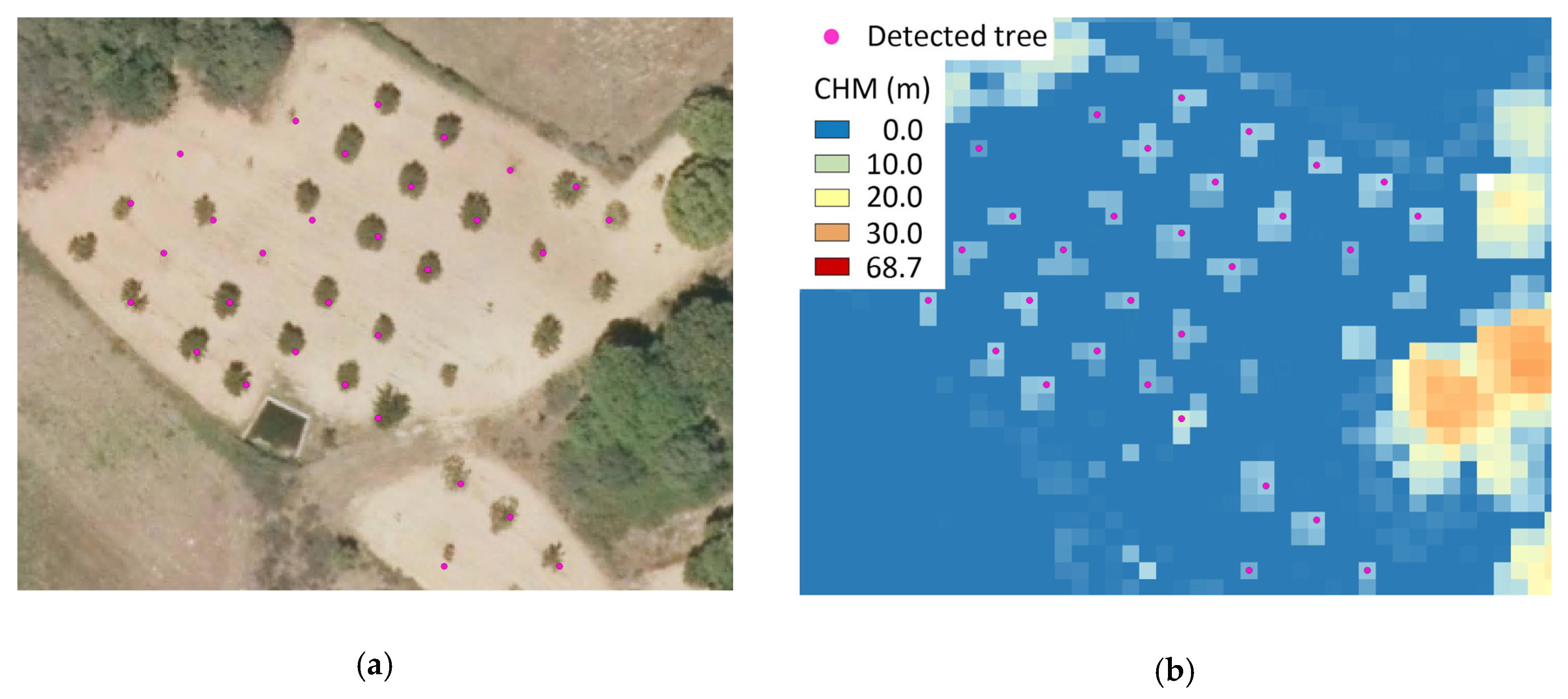
The goal of our research is to explore the potential of the combination of Sentinel-2 satellite images with airborne LiDAR data in the detection, mapping, and characterization of small plantations of trees on a large scale. We used open-access data, specifically data provided by the Copernicus Earth Observation Program and the LiDAR National database [39]. We adopted the chestnut plantations (Castanea sativa) of Galicia, a region in northwestern Spain, as a case study. In this region, chestnut plantations have been increasing recently and becoming an important source of income for the area. However, there is no official record of plantations’ locations and characteristics. Sentinel 2 channels and LiDAR derived statistics are processed using supervised classification algorithms in order to locate the small parcels covered by chestnut plantations. Upon location, we performed individual tree detection (ITD) and tree height estimation by applying a local maxima algorithm to a LiDAR derived Canopy Height Model (CHM). We also calculated the crown surface of individual trees by applying a method based on two-dimensional (2D) tree shape reconstruction and canopy segmentation to a projection of the LiDAR point cloud.

2. Materials and Methods

2.1. Case Study

The present study addresses the described objectives using chestnut tree plantations as a case study. Since the 19th century, chestnut cultivation has been progressively abandoned in Europe due to the propagation of the pathogen Phytophthora spp. (ink disease) [42] and to the progressive depopulation of rural areas that began in the last quarter of the 20th century [43]. This decline has lately been accelerated by the wound-parasite Cryphonectria parasitica (chestnut blight) [42]. Current stands are being affected by an outbreak of Dryocosmus kuriphilus [44]. Chestnuts have been used as a staple food, and chestnut wood was commonly used to make house frames and furniture, for tannin production, and as a source of firewood [45,46]. In recent decades, the plantations for wood and nut production are becoming viable once again due to the attenuation of blight severity owing to the introduction of hypovirulent strains of the chestnut blight [47], as well as to genetic variation involving resistance to ink disease [48].

Regardless, the sweet chestnut covers more than 2.5 million ha in Europe [46,49]. The nut production in Spain accounts for 8.3% of the European market, and Galicia accounts for 65.9% of the Spanish market [50]. The Galician Forest Plan foresees the planting of 20,000 additional hectares in the coming decade [51]. The reforestation process will be promoted through subsides to private landowners [52]. Thus, the recovery of Galician chestnut plantations and the monitoring of these plantations should be accomplished as efficiently and accurately as possible. Prada et al. [53] have recently confirmed the need to improve the current decision-making tools surrounding these plantations.

The present study was performed over the entirety of the municipality of Riós, Galicia (Figure 1). It has an area of 114.4 km², in which the elevation ranges from 700 to 975 m [54]. The chestnut plantations of Riós constitute a representative case study since they have been increasing and becoming an important source of income in the local economy in recent years. However, there is no official census of their location, area, or number, nor of the characteristics of their trees. An analysis of the cadaster [55] revealed that in Riós, the agricultural and forest plots’ mean size is 0.1 ha and their mode size is 0.17 ha. The parcels covered by chestnut plantations are scattered throughout the whole municipality and interspersed among parcels with different forest/agricultural land cover. All plantations have a similar pattern, trees are planted in lines, exhibit homogeneous tree spacing, and there is no canopy closure. Figure 2a presents plots’ distributions and sizes in the study area. Figure 2b shows a detailed view of an example of the structure of a plantation.

2.2. Data Acquisition and Preprocessing

We used Sentinel-2 images as the source of spectral information. Sentinel-2 is a team of twin satellites developed by the European Space Agency (ESA) for the operational needs of Copernicus, the European system of Earth monitoring [19]. They sample 13 spectral bands, providing a spatial resolution, which ranges from 10 m to 60 m [19]. Their mean orbital altitude is 786 km; their orbit inclination is 98.62°; and their geographical coverage extends from 56° South to 83° North. The Radiometric resolution of the images is 12 bits, enabling the detection of 4096 potential light intensity values [19]. Their spectral bands’ specifications are listed in

Table 1. Specifications of spectral bands provided by Sentinel [19].

Band	Central Wavelength (nm)	Bandwidth (nm)	Spatial Resolution (m)	Code
Band 1—Coastal aerosol	443	20	60	B01
Band 2—Blue	490	65	10	B02
Band 3—Green	560	35	10	B03
Band 4—Red	665	30	10	B04
Band 5—Near Infrared (NIR)	705	15	20	B05
Band 6—NIR	740	15	20	B06
Band 7—NIR	783	20	20	B07
Band 8—NIR	842	115	10	B08
Band 8A—NIR narrow	865	20	20	B8A
Band 9—Water vapor	945	20	60	B09
Band 10—Shortwave Infrared (SWIR) (cirrus)	1375	30	60	B10
Band 11—SWIR	1610	90	20	B11
Band 12—SWIR	2190	180	20	B12

.

We used the Sentinel-2 Level-2A product. It includes radiometric, geometric, and atmospheric corrections. We chose the image dated 16/03/2019 due to the absence of clouds and shadows on that day as well as to the phenological stage of the vegetation, which favored discrimination between different land covers.

We obtained LiDAR point-clouds that covered the whole study area from the free repository of geographical information from the Spanish National Air Orthophotography Program (PNOA by its initials in Spanish) [56]. Data was acquired in 2016 using an airborne laser scanner (ALS) with a LEICA ALS80 sensor, obtaining a nominal point density of 0.5 points/m². The data was georeferenced in the ETRS89 system with a Root Mean Square Error (RMSE) of 0.3 m in the horizontal directions and 0.2 m in the vertical directions [56].

We downloaded LiDAR point clouds for the whole study area and pre-processed them using LasTools software [57]. We classified the LiDAR point clouds to label the points that corresponded with the ground using lasground. We then estimated the height of each point above the ground. This step, which was performed using lasheight, allowed the point cloud to be normalized.

Figure 3 shows the front view of the normalized LiDAR point cloud for a chestnut plantation line. From the profile, it is possible to see how the low density of the LiDAR provides a discontinuous point cloud for chestnut trees. The point cloud contains just ground and canopy returns due to the absence of a shrub layer. Given the low density of the point cloud, stems are not detected.

2.3. Detection of Chestnut Plantations

The goal of this step was to locate the chestnut plantations in the study area through supervised classification. An overview of the procedure we followed is presented in Figure 4. Supervised classification algorithms allow data classification after a prior learning process using training data. This approach has been thoroughly and successfully used in land-cover-classification-related studies [58,59,60]. We aimed to classify the study area into two classes, “chestnut” (chestnut plantations), and “other”. The “other” class includes the main land covers besides chestnut crops: conifer forests, broadleaf forests, other crops, anthropogenic areas, rocky areas, and shrublands. Three different algorithms have been tested and compared: Random Forest (RF) [61], Support Vector Machine (SVM) [62], and XGBoost [63], to evaluate the performance of some state-of-the-art algorithms [64,65]. Following is presented a small description of each algorithm.

• Random Forest (RF) is a classifier consisting of a collection of tree-structured classifiers, combined such that each tree depends on the values of a random vector sampled independently and with the same distribution for all trees in the forest [61]. The outputting class is the mode of the classes of the individual trees [61].
• The SVM training algorithm aims to find the optimal hyperplane that separates the dataset into a discrete predefined number of classes. The term optimal separation hyperplane is the decision boundary that minimizes misclassifications, obtained in the training step. The hyperplane boundary can be defined using different kernels. A detailed mathematical description of a SVM can be found in Cortes and Vapnik [62].
• XGBoost is a scalable end-to-end tree boosting system that improves the classical gradient boosting machine (GBM). The GBM builds an additive model of weak learners (decision trees) and then generalizes them by optimizing an arbitrarily defined loss function to make stronger predictions [66]. XGBoost improvement is that the algorithm simultaneously optimizes the loss function while building the additive model. A detailed description of XGBoost can be found in Chen and Guestrin [63].

We selected Sentinel-2 bands and LiDAR-derived statistics as the predictive variables to perform the supervised classification. Predictive variables were in raster format. Considering that our research is focused on small parcels, we considered only the Sentinel-2 bands with 10 or 20 m of spatial resolution: bands 2, 3, 4, 5, 6, 7, 8, 8A, 11, 12. In order to perform the classification the different bands must have the same resolution. We decided to resample 10 m to 20 m bands since the methodology is designed to be applied over large study areas (at the state or country level), therefore we seek to decrease computing time and storage capacity as much as possible.

In order to obtain LiDAR derived predictive variables we transformed LiDAR point clouds into different raster images with information from point-cloud statistical variables. These variables were selected to represent the geometric characteristics that would allow for the differentiation between chestnut plantations and other land-covers. The variables that we obtained were parameters related to the vegetation’s vertical structure, and its height and canopy density characteristics. We also considered shrub density since chestnut plantations are characterized by an absence of vegetation below 2 m, while some other covers can present varying densities and recovery of shrubs.

In order to perform the combined analysis using Sentinel-2 bands and LiDAR-derived statistics, the later ones were transformed into raster channels with the same spatial resolution than the former ones. For this end, we created a grid with 20 m spatial resolution. We performed a voxelization of the normalized LiDAR point cloud considering voxels with the grid cell size as bottom base and the height that was selected for every statistical variable. The value of every statistical parameter was obtained for every voxel, and assigned to the corresponding grid cell. The procedure was fully carried out with LasTools software [57]. As a result, of this process, a single raster image was obtained for every LiDAR derived statistic. The selected LiDAR variables and the method followed to calculate them are listed below (a summary is shown in

Table 2. Calculated LiDAR metrics.

Variable	Description	Code
CHM (Canopy Height Model)	Maximum height above ground	high
Average	Average height above ground	avg
Standard deviation	Standard deviation of all points’ height	stdv
50th Percentile	50th percentile for height	P50
90th Percentile	90th percentile for height	P90
Shrub density	Number of points between 0.5 m and 2 m divided by the total number of returns below 2 m	shrub
Canopy base height	Lowest height above DBH (1.37 m)	c_min
Average canopy height	Average height above DBH	c_avg
Canopy standard deviation	Standard deviation of points above height of DBH	c_stdv
Canopy cover	Number of first returns above DBH divided by the number of all first returns	c_cov
Canopy density	Number of points above DBH divided by the total number of returns	c_dns
Canopy kurtsosis	Canopy height kurtosis	c_ku
Canopy skewness	Canopy height skewness	c_ske

):

• maximum height above ground: each raster cell contains the elevation value of the highest point within the cell. We computed it using the tool lasgrid;
• average height above ground: each raster cell contains the average height value of the points within the cell. We computed it using the tool lasgrid;
• standard deviation of all point’s height: each raster cell contains the standard deviation value of the height values of all points within the cell. We computed it using the tool lasgrid;
• 50th percentile: each raster cell value is the height percentile 50th computed among all the points within the cell. We computed it using the tool lascanopy;
• 90th percentile: each raster cell value is the height percentile 90th computed among all the points within the cell. We computed it using the tool lascanopy;
• canopy base height: each raster cell values is the minimum elevation value above Diameter Base Height (DBH) among all the points within the grid. We adopted a DBH of 1.37 m. We computed it using the tool lascanopy;
• average canopy height: each raster cell value is the average elevation value of all the points within the cell above the DBH. We computed it using the tool lascanopy;
• canopy standard deviation: each raster cell value is the standard deviation of the elevation values of all the points within the cell above the DBH. We computed it using the tool lascanopy;
• canopy cover: each raster cell value is the number of first returns above the DBH divided by the number of all first returns of all the points within the cell. We computed it using the tool lascanopy;
• canopy density: each raster cell value is the number of points above the DBH divided by the total number of returns among all the points within the cell. We computed it using the tool lascanopy;
• canopy kurtosis: each raster cell value is the kurtosis computed for all the elevation values of the points above the DBH within the cell. We computed it using the tool lascanopy;
• canopy skewness: each raster cell value is the skewness computed for all the elevation values of the points above the DBH within the cell. We computed it using the tool lascanopy;
• shrub density: first, we classified the normalized point cloud into strata. We considered points below 0.15 m as ground points; points from 0.15 m to 0.5 m as low vegetation points; points from 0.5 m to 2 m as shrub points; and points above 2 m as high vegetation points. Next, we drop all the points above 2 m to obtain a normalized point cloud free of high vegetation points. The two steps were performed using lasclassify. Finally, on the normalized point cloud without the high vegetation points, we calculated the shrub density for each cell. This density value is the number of points above 0.5 m divided by the total number of points within the cell. We computed it using lascanopy.

As aforementioned, supervised classification relies on training areas of the classification classes. We defined them through photointerpretation of aerial images provided by PNOA [56] (pixel size of 0.22–0.45 m). In the aerial image, we manually delineated a total of 46 polygons corresponding to the “chestnut” class and 24 corresponding to the “other” class. We then extracted the values of all the pixels contained in those polygons for all of the predictive raster images described above. A total of 1005 pixel values were obtained for the “chestnut” class and a total of 1880 for the “other” class.

With this training set we built a first model (Model 1) using the RF algorithm of the Random Forest package for the R software [67]. We used the default parameters after observing in several tests that changing them hardly changed the algorithm’s performance.

Afterwards, in order to exclude correlated variables and variables that did not contribute to prediction, we performed a variable selection using the Variable Selection Using Random Forests (VSURF) R package [68]. VSURF variable selection is based on RF. On a first step (preliminary elimination and ranking), it ranks the variables according to a variable importance measure (typically averaged over 50 RF runs) and eliminates the unimportant ones. A description of the variable importance measure can be found in Genuer et al. [68]. On a second step, selection of variables is performed. First, the algorithm constructs a nested collection of RF models and selects the variables of the model leading to the smallest out-of-bag error (OOB): the classification error directly provided by the RF algorithm [61]. Second, based in the variables selected on the previous stage, it constructs an ascending sequence of RF models, by invoking and testing the variables in a stepwise way. The variables of the last model are finally the selected ones. A more detailed description of the VSURF package strategy can be found in Genuer et al. [68]. A new model was created with the selected variables. Three different algorithms were used. Firstly, we used RF. We compared the two models obtained with RF (Model 1 with all the variables and Model 2 with selected variables) in order to select the most efficient one in terms of predictive-variable needs, computation time and accuracy. We based our selection on the OOB estimator. We also calculated variables’ importance, based on their Mean decrease in Gini [69], in order to find out which variables were most valuable in the prediction.

Two additional algorithms were evaluated, using in both cases the same training set as the one used to create Model 2: SVM (Model 3) and XGBoost (Model 4). We applied the SVM algorithm through the library e1071 [70] using default parameters. To apply the XGBoost algorithm we used the R library XGBoost [71]. The step size of each boosting step was 0.3, the maximum depth of the tree was 5, the number of threads used in the training were 2 and the number of interactions 200.

2.4. ITD in Chestnut Plantations

We performed the ITD using a raster-based method. CHM-based ITD methods are the most commonly used in ITD studies [72]. They are robust methods, especially if the focus is the top-most canopy [73], although there is a lack of tree-detection studies in broadleaves [72]. To detect the individual trees in a CHM, local maxima algorithms are used. Local maxima algorithms identify the pixel with the highest value within a specified neighborhood of pixels. Apart from determining tree position, tree height is also obtained.

In order to perform this process, we created a CHM for the whole study area using LasTools software [57]. Several CHMs with different resolutions (1 m, 2 m, and 5 m) were created to choose the most suitable resolution for applying ITD on chestnuts plantations. The CHMs were overlapped with the high-resolution PNOA images [56] in order to, through visual interpretation, asses which resolution best represented the chestnut crown’s shape. We observed that 5 m produced an excessive generalization of the canopies while 1 m and 2 m CHMs better matched with the tree crowns. Between these two options, we decided to choose the coarsest resolution (2 m). We then located the CHM maxima by applying the SAGA Local Maxima algorithm [74]. Considering that the minimum height of plantation trees is 2 m, we filtered the local maxima by selecting only those with a z value that exceeded 2 m. Finally, we extracted those identified points, which belonged to the areas previously classified as plantations.

2.5. Characterization of Chestnut Plantations

For the characterization of chestnut trees, we focused on individual tree height and crown surface calculations. By implementing the process described in the previous section, we obtained a set of points with x-y coordinates, which corresponded to chestnut individuals. We obtained the height of each point from its corresponding position in the CHM.

The next step was to calculate the crown surface for each individual. Research regarding ITD in broadleaves is scarce. The most common methods are based on point cloud analysis [73]. These methods require high point density (e.g., >10 points/m²) LiDAR data [73] that allows for the full reconstruction of individual trees. Due to the fact that the data used in this case study was low density, we decided to apply a method based on 2D tree shape reconstruction and canopy segmentation. We segmented the canopy point cloud using DBH as the height cut-off. We then projected it orthogonally. Given that in most of the plantations in the study area there is no canopy closure between contiguous trees, canopy points are grouped, meaning that each group of points corresponds to one individual tree. In order to automate the process of canopy delineation, we clustered the orthogonally projected points into individual trees. This step was possible thanks to the absence of canopy closure and to the regular tree spacing. Clustering was based on buffering the points obtained in the ITD process. The buffer might be smaller than the tree spacing. Crown 2D shape reconstruction involved creating a convex-hull around the orthogonal projection of the points belonging to each individual tree. The Convex-hull algorithm establishes the smallest convex polygon that contains all of the points in a given set of points in a plane. The application of the convex-hull allowed us to construct polygons that corresponded to the contours of the projected canopy for each tree in a chestnut plantation. We used the polygons to estimate the area of the canopy’s orthogonal projection on the ground for every tree.

2.6. Assessment of Accuracy

In order to assess the accuracy in the detection of plantations we created a random sample of 600 points within the whole municipality of Riós. We divided these points evenly into plantations and other land cover areas. We obtained the current land cover of those points through a visual interpretation of PNOA orthophotos [56]. Afterwards, we created a confusion matrix relating the real class with the class obtained from the different algorithms. In these confusion matrices, we calculated the overall accuracy, the user’s accuracy and the producer’s accuracy.

The ITD detection accuracy was evaluated for 50 plots that were randomly selected from within the whole study area. In these plots, we compared the number of detected trees to the real number of trees in order to estimate various parameters at the plot level: the detection rate (number of detected trees divided by real number of trees), the detection accuracy (number of true positives divided by the real number of trees), the omission error (number of false negatives divided by number of detected trees), and the commission error (number of false positives divided by the number of detected trees). We obtained the real number of trees and their location through visual interpretation of the PNOA orthophotos [56]. Finally, we calculated the average values of these plot metrics to obtain the final accuracy metrics.

In addition, we evaluated the characterization metrics for trees. In order to assess tree height accuracy, we measured 60 randomly selected trees directly on the LiDAR point cloud. The z of the highest canopy point of each tree was considered the true height of the tree. By creating a linear regression between the observed and predicted values, we were able to obtain a set of values to give us an idea of the prediction accuracy (slope, coefficient of determination R², bias, and RMSE). To assess the accuracy of the crown surface calculation, we manually delineated 60 trees on the PNOA orthophotos [56]. We compared the surface obtained using the delineated polygons with the surface obtained using the convex hull algorithm. We carried out the same statistical tests to assess the accuracy of the calculated crown surfaces.

3. Results

3.1. Detection of Chestnut Plantations

We applied the described methodology, based on applying the RF algorithm to multispectral images and LiDAR based statistics, to obtain a map of the chestnut plantations in the Municipality of Riós.

We obtained and analyzed Model 1 using radiometric and LiDAR variables. This model had an OOB error of 5.93% (see

Table 3. Training data classification results for Model 1, including the out-of-bag (OOB) error. Model created using Random Forest (RF). Predictive variables were all of the obtained variables.

Training Data/Classification	Chestnut Pixels	Others Pixels	Class Error	OOB
Chestnut pixels	917	88	0.087
Others pixels	83	1797	0.044
				5.93%

). The most relevant prediction variables for this model were bands corresponding to the red edge, the infrared and the SWIR regions of the electromagnetic spectrum, together with information about the shrub layer, vegetation height and canopy density (see Figure 5).

The variable selection was performed using the VSURF algorithm. It revealed that the optimum variables for prediction were B05, B8A, P50, c_dns, scrub, B08, B11, P90, and B12. We created a simplified model including only these variables (Model 2). In this model, the predictive variables were reduced by 63% and computation time for the algorithm also decreased. The Red edge and the 50th percentile were the variables that had the most influence on the prediction (see Figure 6). Model 2 had an OOB of 5.62% (see

Table 4. Training data classification results for Model 2, including the out-of-bag (OOB) error. Model created using RF. Predictive variables, variables selected by the selection algorithm (VSURF).

Training Data/Classification	Chestnut Pixels	Others Pixels	Class Error	OOB
Chestnut pixels	929	76	0.075
Others pixels	86	1794	0.045
				5.62%

), which is slightly lower than the OOB for model 1.

Taking these results into account, we applied Model 2 to the entire study area, which yielded 1360.4 hectares of chestnut plantations. Figure 7 shows an example of the prediction results.

We obtained the accuracy of the predictions with the 600 points that were randomly created (Section 2.6). Model 2 yielded an overall accuracy of 95.67%. User and producer accuracies are in the 90% range as well (

Table 5. Evaluation of chestnut plantation area predictions obtained using Model 2 (model created by applying Random Forest). Ground truth data were created with a random stratified sample of 600 points.

Real/Classif.	Other	Plantation	Total	Producer’s Accuracy
Other	286	14	300	95.33%
Plantation	12	288	300	96.00%
Total	298	302	600
User’s Accuracy	95.97%	95.36%		Overall Accuracy: 95.67%

). Similar values were obtained for Models 3 and 4, which are reported in

Table 6. Evaluation of chestnut plantation area predictions obtained using Model 3 (model created applying SVM). Ground truth data were created with a random stratified sample of 600 points.

Real/Classif.	Other	Plantation	Total	Producer’s Accuracy
Other	269	31	300	89.67%
Plantation	12	288	300	96.00%
Total	281	319	600
User’s Accuracy	95.73%	90.28%		Overall Accuracy: 92.83%

and

Table 7. Evaluation of chestnut plantation area predictions obtained using Model 4 (model created applying XGBoost). Ground truth data were created with a random stratified sample of 600 points.

Real/Classif.	Other	Plantation	Total	Producer’s Accuracy
Other	271	29	300	90.33%
Plantation	11	289	300	96.33%
Total	282	318	600
User’s Accuracy	96.00%	90.28%		Overall Accuracy: 95.16%

, respectively.

Although all of the algorithms have a great performance, analyzing the raster obtained prediction, we observed that there are overdetection errors. These errors appear no matter which algorithm is used. An example of areas wrongly classified as plantations by the RF algorithm is shown in Figure 8.

3.2. Chestnut Tree Detection in Plantations

In order to detect individual trees in chestnut plantations, a CHM was generated for the whole study area. Taking into account the average size of chestnut trees, we used a CHM resolution of 2 m. We applied the local maxima algorithm, and executed the filtering step, as described in the previous section. As a result, 57,981 trees were identified. Figure 9 shows an example of the trees detected in a parcel. ITD accuracy results are shown in

Table 8. Summary of accuracy assessment results for individual tree detection.

Detection Rate (DR)	Detection Accuracy (DA)	Omission Error (OE)	Commission Error (CE)
96%	90%	16%	6%

. According to our results, the number of trees in each parcel can be detected with an average error of 4% (a detection rate of 96%). However, the detection accuracy is 90%, meaning that 6% of the detected trees do not correspond to real trees (commission error).

3.3. Chestnut Characterization

The individual tree detection allowed us to associate a height value to each individual tree detected. We estimated tree height for all detected trees. The mean height value for all of the located points was 5.74 m, whereas the maximum and the minimum values were 38.35 m and 2.00 m, respectively. These values had a standard deviation of 2.69 m. Height accuracy results are shown in Figure 10. There is a great correlation between observed and predicted values (R² = 0.83). The RMSE was 0.5 m.

The application of the described 2D delineation method allowed us to obtain a set of polygons, which we used to estimate tree crown surfaces. The results of each of the steps in the process are shown in Figure 11.

Results of the assessment of the accuracy in tree surface estimation are shown in Figure 12. In this case, the correlation was lower (R² = 0.74) and the bias was higher (4.34). The RMSE was 6.39 m².

4. Discussion

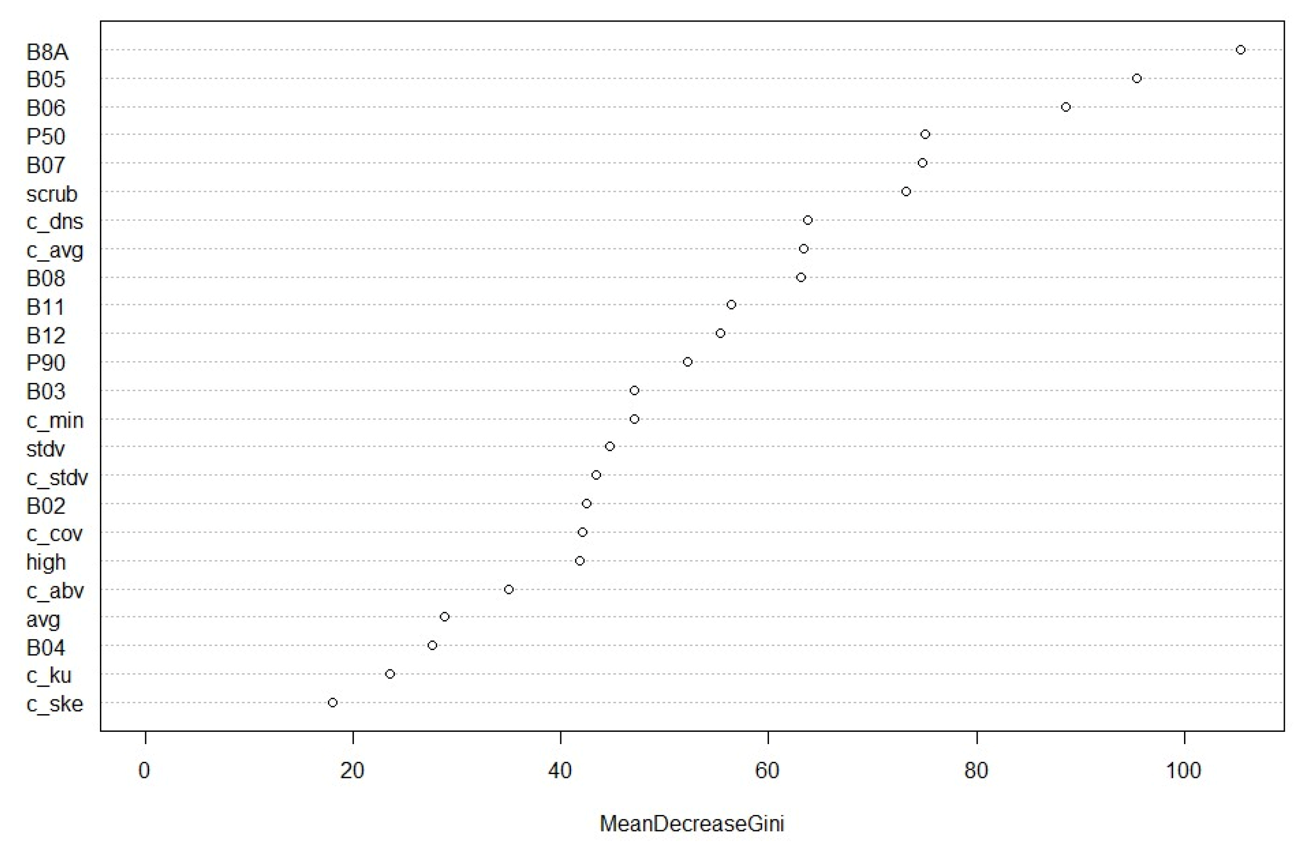
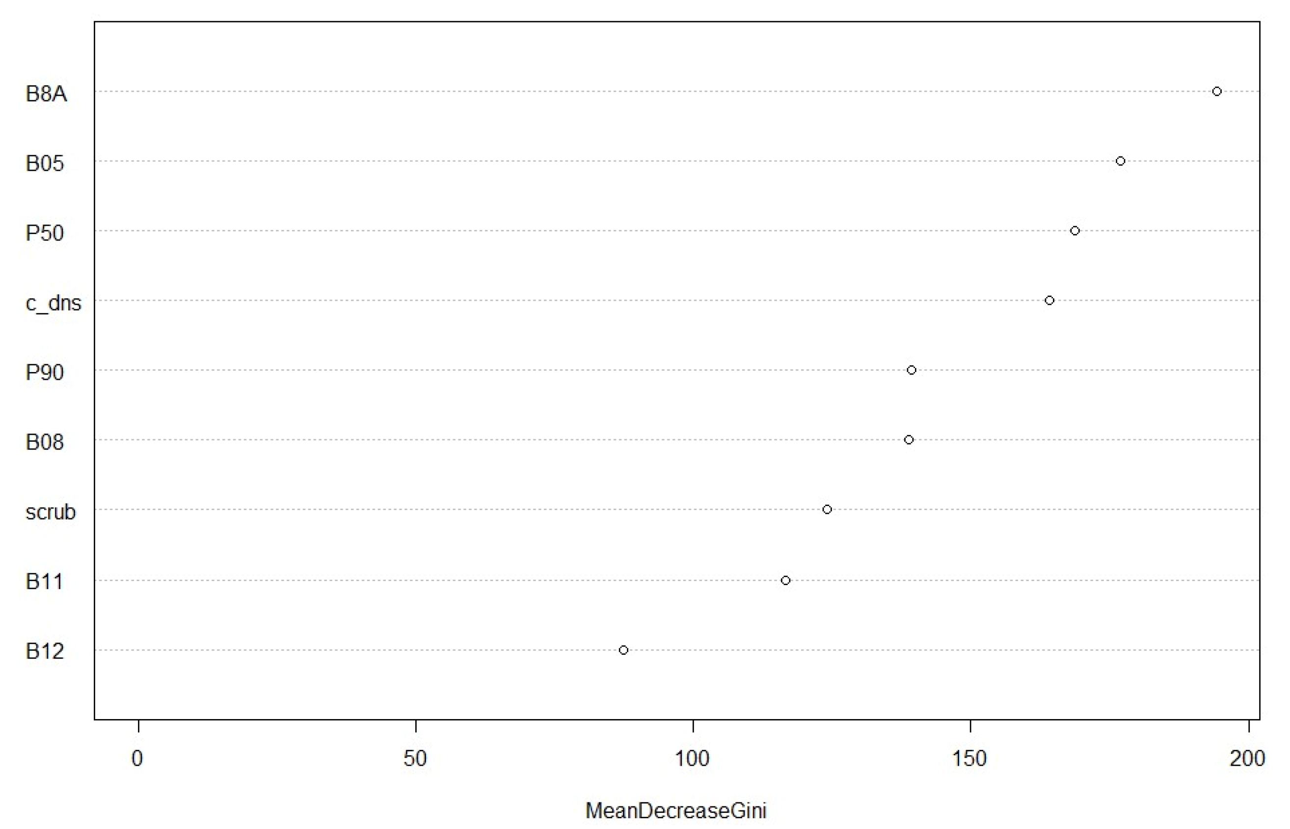
The present study identifies small parcels planted with chestnut trees using LiDAR statistics and Sentinel-2 data with a high overall accuracy. The obtained results reveal that the reduction in the number of variables: a decrease to nine variables (five Sentinel-2 bands and four LiDAR derived statistics) does not significantly compromise the accuracy of the results. Furthermore, the supervised classification algorithm is not a determinant feature in accuracy metrics: it ranges from 92% to 95%. The SVM model is the one that yields the lowest accuracy levels, while the RF provide the highest values. Several other studies report similar results [64,75] indicating that the choice of the classifier itself is often of low importance if the data is adequately pre-processed to match the requirements of the classifier [65].

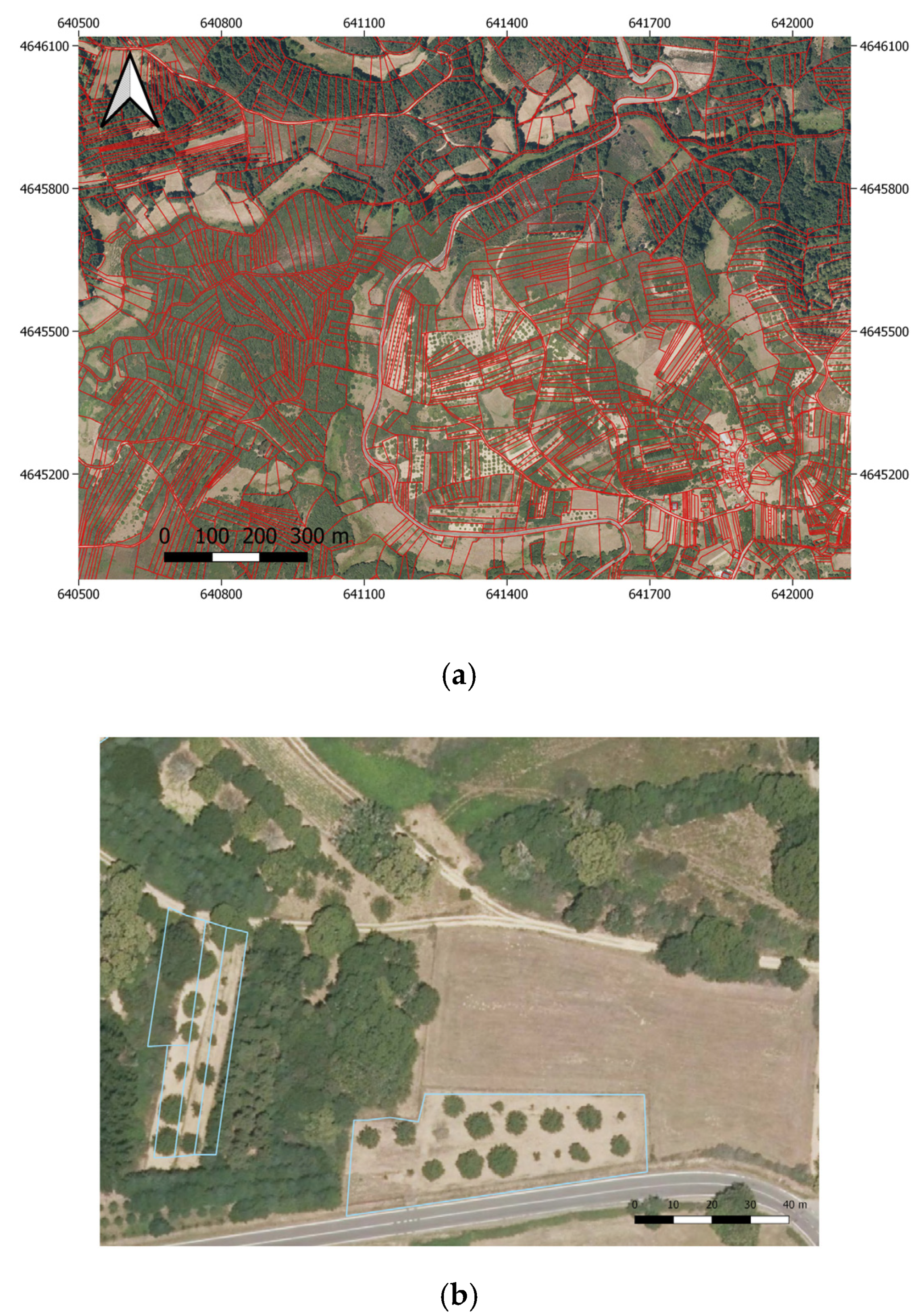
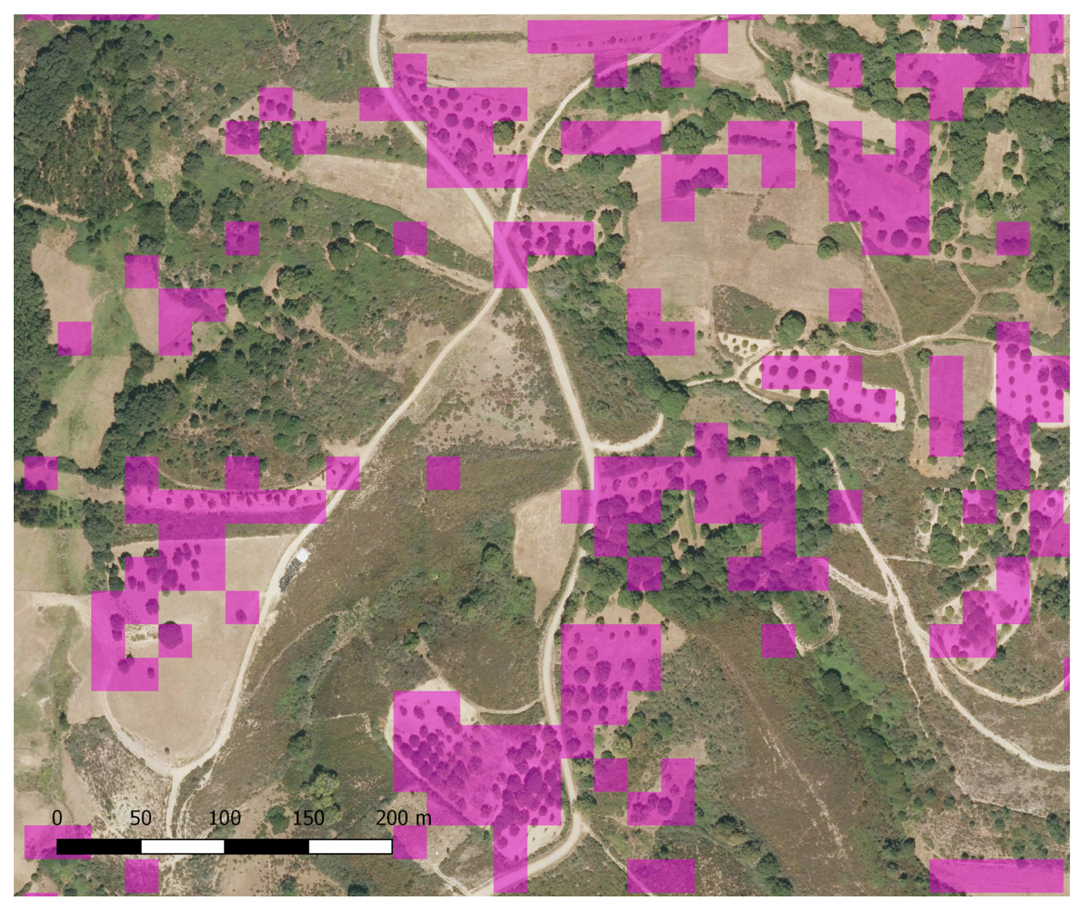
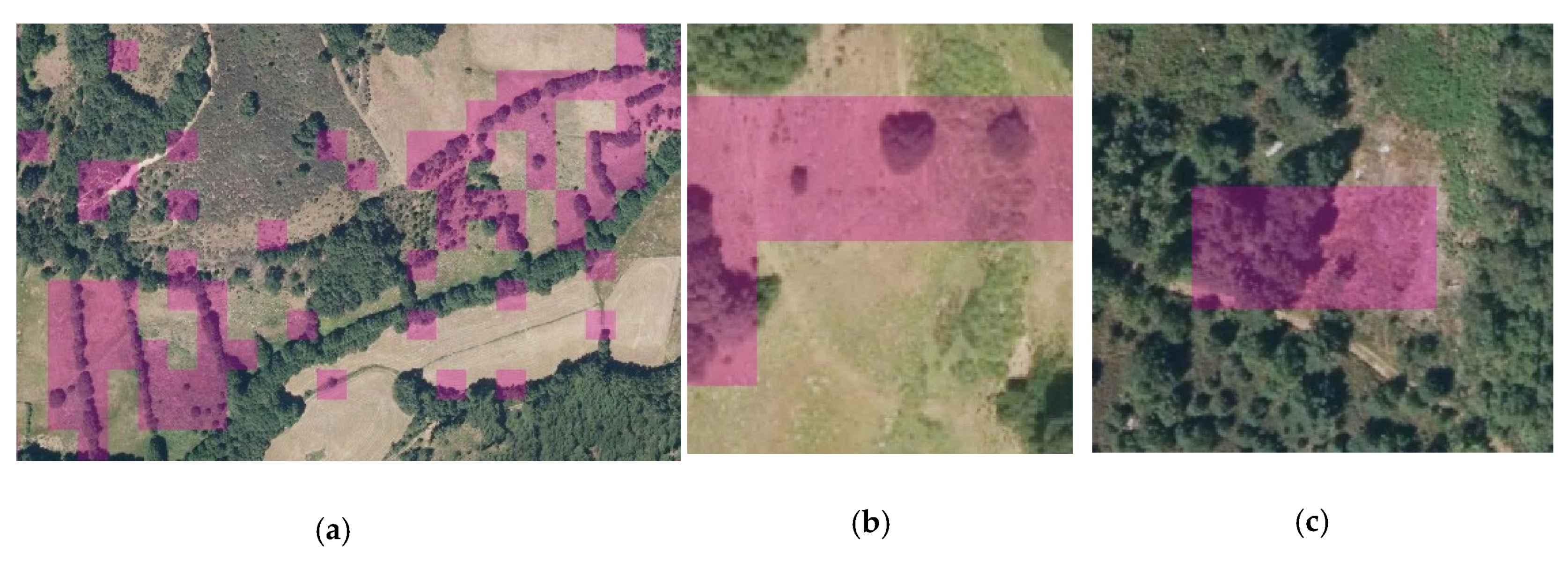
Despite the high detection accuracy, an overestimation of total chestnut plantation area was observed (Figure 8). This is due to the peculiarities of the rural environment in the study area. Tree lines and hedges are commonly used to mark parcel boundaries; native species are used, chestnut being one of them. Consequently, the radiometric behavior of these features is often similar to that of plantations. Furthermore, these boundaries also have similar geometric patterns to chestnut plantations: absence of a shrub layer, and analogous tree spacing and canopy density. Isolated trees and forest edges are often erroneously mapped as plantations as well. These are the main causes of the overestimation. However, additional errors, due to the resolution of the source data, often arise when the plantations to be detected are small and irregularly shaped. The result is often a coarse plantation boundary. The area of one square pixel may be mostly an elongated plantation parcel, but it will inevitably include the contiguous surrounding areas, which may exhibit different land usages (Figure 7).

The particular structure of the plantations analyzed is what makes LiDAR decisive for plantation detection. However, the presented methodology may not be valid if the stand structure changes, especially if there is canopy closure or shrub layer appears. In that case, the presented methodology would need to be modified. Supervised classification using Sentinel-2 data could be enough as there would not be mixed pixels with mixed radiometry (tree-ground). Alonso et al. detected chestnut forests performing a supervised classification on multi-temporal Sentinel-2 data with a previous reduction of the classification area using LiDAR normalized height [76].

Some other studies have addressed tree plantation detection by combining structural and spectral data obtaining high accuracy levels as well. However, they mainly use high-resolution Satellite data [77,78,79]. The necessity of acquiring high-resolution multispectral data, with its associated costs, could hinder the possibility of performing such studies at a regional or national level.

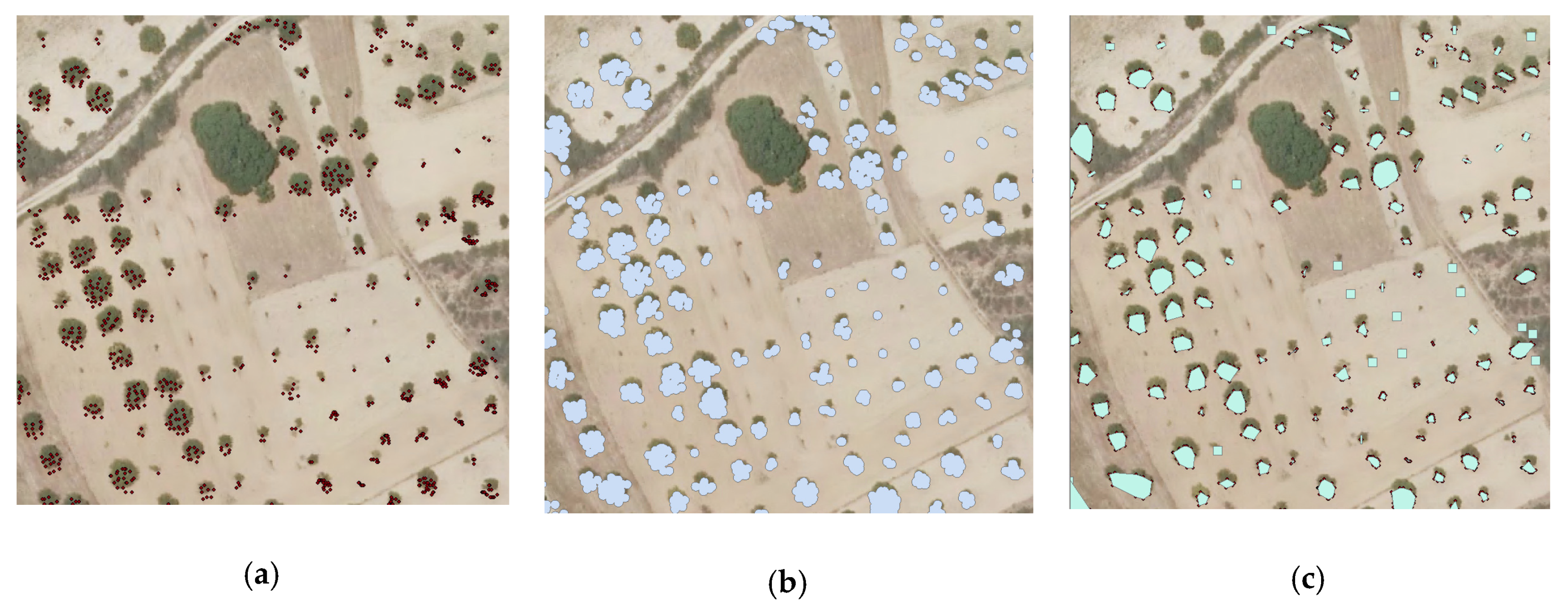
The ITD process allowed us to estimate the total number of chestnut individuals with a detection accuracy of 90%, which constitutes a suitable value for management purposes. However, some errors were detected. Most of them were related to the overestimation of chestnut plantation area. Since the ITD process is applied to the areas that have been previously mapped as plantations, any errors in the delimitation of their boundaries lead to errors in the counting of chestnut trees. An improvement of the detection method will be needed to avoid that type of errors. Furthermore, branches, cattle, shrubs, and stones are sometimes detected as false positives. However, canopy closure among trees leads to an underestimation of candidates. Despite these deviations, we obtained high accuracy metrics in the ITD and characterization steps. If we compare our results with the ones obtained by Marques et al., who addressed ITD detection in a very similar study case as the one that we present here (chestnut plantation monitoring) but using UAV-captured images [80], the obtained ITD accuracy is similar (Marques et al. obtained a detection rate of 93.5%). Their approach seams suitable to perform a small-scale study, especially if a National LiDAR database is not available. However, our approach will enable the monitoring of a large area due to the lack of costs and feasibility to have information about the whole territory derived from the use of a National LiDAR dataset.

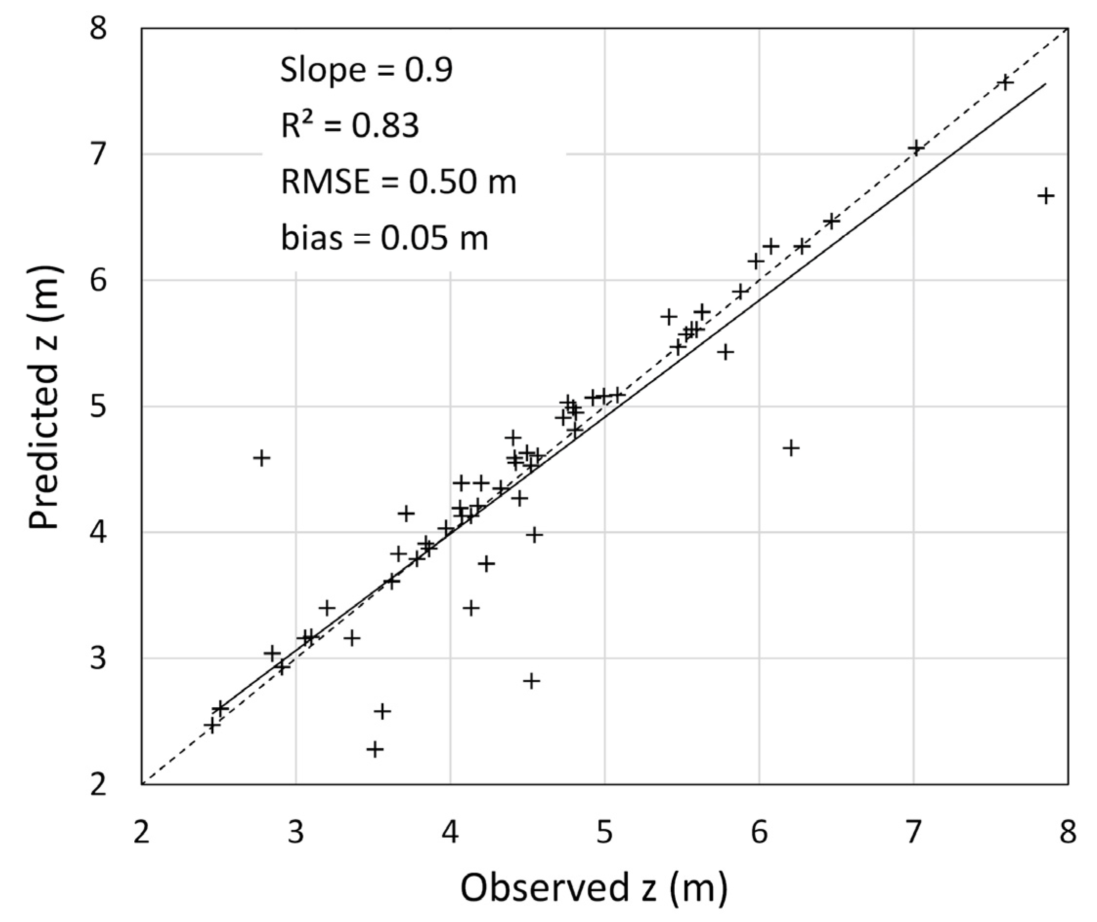
It should be mentioned that and advantage of the method proposed by Marques et al. [80] is that the high resolution of UAV-captured images allowed them to obtain better canopy diameter estimations: a RMSE of 0.44 and an R² of 0.96. The tree height estimation of Marques et al., however, was not better than the estimation that we obtained using the present methodology: R² 0.79, RMSE 0.69. This could be due to the inaccuracy of Structure-from-motion (sfM) techniques on ground reconstruction. These errors are propagated into the estimation of individual tree height [81].

As it was mentioned in the introduction low-density LiDAR is rarely used to characterize individual trees but some studies start to remark the potential of low-density LiDAR for individual tree characterization [36,37,38,41]. The high accurate metrics obtained in this study are another prove of that potential and encourages to continue studying the potential of low-density ALS for individual tree detection and characterization.

Finally, it should be remarked that the results obtained with the methodology proposed in this study demonstrate that the LiDAR PNOA, together with Sentinel data, enables the creation of cartographic products at a Regional or National level that are useful for forest policy makers and forest managers. This go in line with the conclusions about the opportunity that LiDAR PNOA presents to improve Spanish forest made by Gómez et al. [21]. This also agrees with White et al. who have also remarked upon the importance of ALS and open-access satellites data to enhance National forest inventories [20].

5. Conclusions

This study presents a methodology to detect and characterize small plantations of chestnuts. All described processes are based on a combination of low-resolution multispectral data and low-resolution LiDAR point clouds. The multispectral images came from the open-access data from the Sentinel-2 satellite constellation and the LiDAR data came from the open-access database of the Spanish National Mapping Agency.

Using the RF algorithm provided an effective plantation surface estimation, with an overall accuracy of 95.67%. The main limitation observed, which is the coarse delineation of parcel boundaries, is related to the spatial resolution of the satellite images.

ITD through the local maxima algorithm applied to a CHM is an efficient and accurate method for estimating the number of trees in an area and it is powerful enough to locate them. The obtained detection rate and detection accuracy are 96% and 90%, respectively. The limitations in our methods are associated with the previously described error in plantation detection. Our results highlight the need for further research on the potential of low-density LiDAR to assess tree characteristics.

Good forestry policies remain essential for forest managers and are impossible to achieve without thorough knowledge and understanding of resource distribution, extent, and characteristics. This information remains essential in order for policy makers to design policies that are in accordance with the actual situation. The obtained results prove that accurate results useful for forest policy makers and forest managers can be obtained without incurring in high cost products, as it is the case of high-resolution multispectral images or high-resolution LiDAR data. At the same time, the described methodology enables the forest monitoring at a regional or national level, even when the monitoring target consists of very fragmented regions with very small forest parcels scattered around the territory.

References

1. Food and Agriculture Organization of the United Nations (FAO). Voluntary Guidelines on National Forest Monitoring; Food and Agriculture Organization of the United Nations: Rome, Italy, 2017; ISBN 978-92-5-109619-2. [Google Scholar]
2. Bettinger, P.; Boston, K.; Jacek, P.S.; Donald, L.G. Forest Management and Planning, 2nd ed.; Academic Press: Amsterdam, The Netherlands, 2017; Chapter 3. [Google Scholar] [CrossRef]
3. Food and Agriculture Organization of the United Nations (FAO). The State of the World’s Forests (SOFO); Food and Agriculture Organization of the United Nations: Rome, Italy, 2018; ISBN 978-92-5-130561-4. [Google Scholar]
4. Forest Europe. Vision & Mission. Available online: https://foresteurope.org/foresteurope/#1470741557748-134fb529-3b91 (accessed on 2 December 2019).
5. Food and Agriculture Organization of the United Nations (FAO). Strategic Framework on Mediterranean Forests. In Proceedings of the High Level Segment of the Third Mediterranean Forest Week, Tlemcen, Algeria, 17–21 September 2013. [Google Scholar]
6. European Commission Environment. Nature and Biodiversity. Forest Information. Available online: https://ec.europa.eu/environment/forests/information.htm (accessed on 2 December 2019).
7. Ertunç, E.; Çay, T.; Haklı, H. Modeling of reallocation in land consolidation with a hybrid method. Land Use Policy 2018, 76, 754–761. [Google Scholar] [CrossRef]
8. Postek, P.; Leń, P.; Stręk, Ż. The proposed indicator of fragmentation of agricultural land. Ecol. Indic. 2019, 103, 581–588. [Google Scholar] [CrossRef]
9. Ónega-López, F.-J.; Puppim de Oliveira, J.A.; Crecente-Maseda, R. Planning innovations in land management and governance in fragmented rural areas: Two examples from Galicia (Spain). Eur. Plan. Stud. 2010, 18, 755–773. [Google Scholar] [CrossRef]
10. Latruffe, L.; Piet, L. Does land fragmentation affect farm performance? A case study from Brittany, France. Agric. Syst. 2014, 129, 68–80. [Google Scholar] [CrossRef]
11. Ficko, A.; Lidestav, G.; Ní Dhubháin, Á.; Karppinen, H.; Zivojinovic, I.; Westin, K. European private forest owner typologies: A review of methods and use. For. Policy Econ. 2019, 99, 21–31. [Google Scholar] [CrossRef]
12. Hirsch, F.; Schmithüsen, F.J. Private Forest Ownership in Europe; United Nations Economic Commission for Europe (UNECE) and FAO: Geneva, Switzerland, 2010. [Google Scholar] [CrossRef]
13. Surový, P.; Kuželka, K.; Surovỳ, P.; Kuželka, K. Acquisition of forest attributes for decision support at the forest enterprise level using remote-sensing techniques—A review. Forests 2019, 10, 273. [Google Scholar] [CrossRef] [Green Version]
14. Koskinen, J.; Leinonen, U.; Vollrath, A.; Ortmann, A.; Lindquist, E.; d’Annunzio, R.; Pekkarinen, A.; Käyhkö, N. Participatory mapping of forest plantations with Open Foris and Google Earth Engine. ISPRS J. Photogramm. Remote Sens. 2019, 148, 63–74. [Google Scholar] [CrossRef]
15. Picos, J.; Alonso, L.; Bastos, G.; Armesto, J. Event-based integrated assessment of environmental variables and wildfire weverity through Sentinel-2 data. Forests 2019, 10, 1021. [Google Scholar] [CrossRef] [Green Version]
16. Masek, J.G.; Hayes, D.J.; Joseph Hughes, M.; Healey, S.P.; Turner, D.P. The role of remote sensing in process-scaling studies of managed forest ecosystems. For. Ecol. Manag. 2015, 355, 109–123. [Google Scholar] [CrossRef] [Green Version]
17. Boyd, D.S.; Danson, F.M. Satellite remote sensing of forest resources: Three decades of research development. Prog. Phys. Geogr. 2005, 29, 1–26. [Google Scholar] [CrossRef]
18. Roy, D.P.; Wulder, M.A.; Loveland, T.R.; Woodcock, C.E.; Allen, R.G.; Anderson, M.C.; Helder, D.; Irons, J.R.; Johnson, D.M.; Kennedy, R.; et al. Landsat-8: Science and product vision for terrestrial global change research. Remote Sens. Environ. 2014, 145, 154–172. [Google Scholar] [CrossRef] [Green Version]
19. European Space Agency (ESA). ESA Standard Document—Sentinel-2 User Handbook. 2015. Available online: https://sentinel.esa.int/documents/247904/685211/Sentinel-2_User_Handbook (accessed on 19 November 2019).
20. White, J.C.; Coops, N.C.; Wulder, M.A.; Vastaranta, M.; Hilker, T.; Tompalski, P. Remote sensing technologies for enhancing forest inventories: A review. Can. J. Remote Sens. 2016, 42, 619–641. [Google Scholar] [CrossRef] [Green Version]
21. Gómez, C.; Alejandro, P.; Hermosilla, T.; Montes, F.; Pascual, C.; Ruiz, L.A.; Álvarez-Taboada, F.; Tanase, M.; Valbuena, R. Remote sensing for the Spanish forests in the 21st century: A review of advances, needs, and opportunities. For. Syst. 2019, 28, 1. [Google Scholar] [CrossRef]
22. Conrad, C.; Dech, S.; Dubovyk, O.; Fritsch, S.; Klein, D.; Löw, F.; Schorcht, G.; Zeidler, J. Derivation of temporal windows for accurate crop discrimination in heterogeneous croplands of Uzbekistan using multitemporal RapidEye images. Comput. Electron. Agric. 2014, 103, 63–74. [Google Scholar] [CrossRef]
23. Crespin-Boucaud, A.; Lebourgeois, V.; Lo Seen, D.; Castets, M.; Bégué, A. Agriculturally consistent mapping of smallholder farming systems using remote sensing and spatial modelling. Int. Arch. Photogramm. Remote Sens. Spat. Inf. Sci. 2020, XLII–3/W11, 35–42. [Google Scholar] [CrossRef] [Green Version]
24. Apollo Mapping. Available online: https://apollomapping.com/imagery-dem-price-lists (accessed on 29 June 2020).
25. Maes, W.H.; Steppe, K. Perspectives for remote sensing with unmanned aerial vehicles in precision agriculture. Trends Plant Sci. 2019, 24, 152–164. [Google Scholar] [CrossRef] [PubMed]
26. Upadhyay, V.; Kumar, A. Hyperspectral remote sensing of forests: Technological advancements, opportunities and challenges. Earth Sci. Inform. 2018, 11, 487–524. [Google Scholar] [CrossRef]
27. Brosofske, K.D.; Froese, R.E.; Falkowski, M.J.; Banskota, A. A review of methods for mapping and prediction of inventory attributes for operational forest management. For. Sci. 2014, 60, 733–756. [Google Scholar] [CrossRef]
28. Means, J.E.; Acker, S.A.; Harding, D.J.; Blair, J.B.; Lefsky, M.A.; Cohen, W.B.; Harmon, M.E.; McKee, W.A. Use of large-footprint scanning airborne Lidar to estimate forest stand characteristics in the Western Cascades of Oregon. Remote Sens. Environ. 1999, 67, 298–308. [Google Scholar] [CrossRef]
29. Xu, C.; Morgenroth, J.; Manley, B. Mapping net stocked plantation area for small-scale forests in new zealand using integrated rapideye and LiDAR sensors. Forests 2017, 8, 487. [Google Scholar] [CrossRef] [Green Version]
30. Palenichka, R.; Doyon, F.; Lakhssassi, A.; Zaremba, M.B. Multi-scale segmentation of forest areas and tree detection in LiDAR images by the attentive vision method. IEEE J. Sel. Top. Appl. Earth Obs. Remote Sens. 2013, 6, 1313–1323. [Google Scholar] [CrossRef]
31. Wallace, L.; Lucieer, A.; Watson, C.S. Evaluating tree detection and segmentation routines on very high resolution UAV LiDAR data. IEEE Trans. Geosci. Remote Sens. 2014, 52, 7619–7628. [Google Scholar] [CrossRef]
32. Picos, J.; Bastos, G.; Míguez, D.; Alonso, L.; Armesto, J. Individual tree detection in a eucalyptus plantation using Unmanned Aerial Vehicle (UAV)-LiDAR. Remote Sens. 2020, 12, 885. [Google Scholar] [CrossRef] [Green Version]
33. Bouvier, M.; Durrieu, S.; Fournier, R.A.; Renaud, J.P. Generalizing predictive models of forest inventory attributes using an area-based approach with airborne LiDAR data. Remote Sens. Environ. 2015, 156, 322–334. [Google Scholar] [CrossRef]
34. Packalén, P.; Maltamo, M. The k-MSN method for the prediction of species-specific stand attributes using airborne laser scanning and aerial photographs. Remote Sens. Environ. 2007, 109, 328–341. [Google Scholar] [CrossRef]
35. Torresan, C.; Berton, A.; Carotenuto, F.; Di Gennaro, S.F.; Gioli, B.; Matese, A.; Miglietta, F.; Vagnoli, C.; Zaldei, A.; Wallace, L. Forestry applications of UAVs in Europe: A review. Int. J. Remote Sens. 2017, 38, 2427–2447. [Google Scholar] [CrossRef]
36. Parent, J.R.; Volin, J.C.; Civco, D.L. A fully-automated approach to land cover mapping with airborne LiDAR and high resolution multispectral imagery in a forested suburban landscape. ISPRS J. Photogramm. Remote Sens. 2015, 104, 18–29. [Google Scholar] [CrossRef]
37. Mohan, M.; de Mendonça, B.A.F.; Silva, C.A.; Klauberg, C.; de Saboya Ribeiro, A.S.; de Araújo, E.J.G.; Monte, M.A.; Cardil, A. Optimizing individual tree detection accuracy and measuring forest uniformity in coconut (Cocos nucifera L.) plantations using airborne laser scanning. Ecol. Model. 2019, 409, 108736. [Google Scholar] [CrossRef]
38. Kathuria, A.; Turner, R.; Stone, C.; Duque-Lazo, J.; West, R. Development of an automated individual tree detection model using point cloud LiDAR data for accurate tree counts in a Pinus radiata plantation. Aust. For. 2016, 79, 126–136. [Google Scholar] [CrossRef]
39. Gobierno de España. Ministerio de Fomento. Instituto Geográfico Nacional (IGN). Plan Nacional de Ortofotografía Aérea (PNOA) LiDAR. Available online: https://pnoa.ign.es/presentacion (accessed on 28 March 2019).
40. Barrett, F.; McRoberts, R.E.; Tomppo, E.; Cienciala, E.; Waser, L.T. A questionnaire-based review of the operational use of remotely sensed data by national forest inventories. Remote Sens. Environ. 2016, 174, 279–289. [Google Scholar] [CrossRef]
41. Novero, A.U.; Pasaporte, M.S.; Aurelio, R.M.; Madanguit, C.J.G.; Tinoy, M.R.M.; Luayon, M.S.; Oñez, J.P.L.; Daquiado, E.G.B.; Diez, J.M.A.; Ordaneza, J.E.; et al. The use of light detection and ranging (LiDAR) technology and GIS in the assessment and mapping of bioresources in Davao Region, Mindanao Island, Philippines. Remote Sens. Appl. Soc. Environ. 2019, 13, 1–11. [Google Scholar] [CrossRef]
42. de Oliveira, D.; Gomes, A.; Ilharco, F.A.; Manteigas, A.M.; Pinto, J.; Ramalho, J. Importance of insect pollinators for the production in the chestnut, Castanea sativa. In Proceedings of the ISHS Acta Horticulturae 561—VIII International Symposium on Pollination—Pollination: Integrator of Crops and Native Plant Systems; International Society for Horticultural Science (ISHS), Leuven, Belgium, 26 November 2001; pp. 269–273. [Google Scholar] [CrossRef]
43. Zlatanov, T.; Schleppi, P.; Velichkov, I.; Hinkov, G.; Georgieva, M.; Eggertsson, O.; Zlatanova, M.; Vacik, H. Structural diversity of abandoned chestnut (Castanea sativa Mill.) dominated forests: Implications for forest management. For. Ecol. Manag. 2013, 291, 326–335. [Google Scholar] [CrossRef]
44. Avtzis, D.N.; Melika, G.; Matošević, D.; Coyle, D.R. The Asian chestnut gall wasp Dryocosmus kuriphilus: A global invader and a successful case of classical biological control. J. Pest Sci. 2019, 92, 107–115. [Google Scholar] [CrossRef]
45. Álvarez-Lafuente, A.; Benito-Matías, L.F.; Peñuelas-Rubira, J.L.; Suz, L.M. Multi-cropping edible truffles and sweet chestnuts: Production of high-quality Castanea sativa seedlings inoculated with Tuber aestivum, its ecotype T. uncinatum, T. brumale, and T. macrosporum. Mycorrhiza 2018, 28, 29–38. [Google Scholar] [CrossRef] [PubMed]
46. Corredoira, E.; Valladares, S.; Vieitez, A.M.; Ballester, A. Chestnut, European (Castanea sativa). Methods Mol. Biol. 2015, 1224, 163–176. [Google Scholar] [CrossRef]
47. Milgroom, M.G.; Cortesi, P. Biological control of chestnut blight with hypovirulence: A critical analysis. Annu. Rev. Phytopathol. 2004, 42, 311–338. [Google Scholar] [CrossRef] [Green Version]
48. Barakat, A.; Staton, M.; Cheng, C.-H.; Park, J.; Yassin, N.B.M.; Ficklin, S.; Yeh, C.-C.; Hebard, F.; Baier, K.; Powell, W.; et al. Chestnut resistance to the blight disease: Insights from transcriptome analysis. BMC Plant Biol. 2012, 12, 38. [Google Scholar] [CrossRef] [Green Version]
49. Conedera, M.; Manetti, M.; Giudici, F.; Amorini, E. Distribution and economic potential of the Sweet chestnut (Castanea sativa Mill.) in Europe. Ecol. Mediterr. 2004, 30, 179–193. [Google Scholar] [CrossRef]
50. Fandiño Cerqueira, M.E. Hifas Foresta—Hifas da Terra Productos no maderables: Castañas y setas (Spanish). In Proceedings of the Congreso Nacional del Medio Ambiente (CONAMA 2018), Madrid, Spain, 26–29 November 2018. [Google Scholar]
51. Xunta de Galicia. Consellería do Medio Rural. Primera Revisión del Plan Forestal de Galicia. Documento de diagnóstico del monte y el Sector Forestal Gallego (Spanish); Santiago de Compostela, Spain, 2018. Available online: https://mediorural.xunta.gal/sites/default/files/temas/forestal/plan-forestal/1_REVISION_PLAN_FORESTAL_CAST.pdf (accessed on 23 October 2019).
52. Xunta de Galicia—Consellería del Medio Rural Orden de 28 de diciembre de 2018 (Spanish). Diario Oficial de Galicia. 2019, pp. 7572–7617. Available online: http://www.xunta.gal/dog/Publicados/2019/20190201/AnuncioG0426-020119-0001_es.pdf (accessed on 30 October 2019).
53. Prada, M.; González-García, M.; Majada, J.; Martínez-Alonso, C. Development of a dynamic growth model for sweet chestnut coppice: A case study in Northwest Spain. Ecol. Model. 2019, 409, 108761. [Google Scholar] [CrossRef]
54. Concello de Riós. Concello de Riós Introducción (Galician). Available online: http://concelloderios.info/?page_id=2247&lang=es (accessed on 20 June 2020).
55. Gobierno de España. Ministerio de Hacienda. Sede Electrónica del Catastro (Spanish). Available online: https://www.sedecatastro.gob.es (accessed on 3 November 2019).
56. Gobierno de España. Ministerio de Transporte Movilidad y Agenda Urbana Plan Nacional de Ortofotografía Aérea (PNOA) (Spanish). Available online: https://pnoa.ign.es (accessed on 5 October 2019).
57. Martin Isenburg, LAStools—Efficient Tools for LiDAR Processing. Available online: http://lastools.org (accessed on 11 September 2019).
58. Christovam, L.E.; Pessoa, G.G.; Shimabukuro, M.H.; Galo, M.L.B.T.B.T. Land use and land cover classification using hyperspectral imagery: Evaluating the performance of Spectral Angle Mapper, Support Vector Machine and Random Forest. Int. Arch. Photogramm. Remote Sens. Spat. Inf. Sci. 2019, XLII–2/W13, 1841–1847. [Google Scholar] [CrossRef] [Green Version]
59. Pu, R.; Landry, S. Mapping urban tree species by integrating multi-seasonal high resolution pléiades satellite imagery with airborne LiDAR data. Urban For. Urban Green. 2020, 53, 126675. [Google Scholar] [CrossRef]
60. Maxwell, A.E.; Warner, T.A.; Fang, F. Implementation of machine-learning classification in remote sensing: An applied review. Int. J. Remote Sens. 2018, 39, 2784–2817. [Google Scholar] [CrossRef] [Green Version]
61. Breiman, L. Random Forests. Mach. Learn. 2001, 45, 5–32. [Google Scholar] [CrossRef] [Green Version]
62. Cortes, C.; Vapnik, V. Support-vector Networks. Mach. Learn. 1995, 20, 273–297. [Google Scholar] [CrossRef]
63. Chen, T.; Guestrin, C. Xgboost: A Scalable Tree Boosting System. In Proceedings of the 22nd ACM SIGKDD International Conference on Knowledge Discovery and Data Mining, San Francisco, CA, USA, 13–17 August 2016; pp. 785–794. [Google Scholar]
64. Abdi, A.M. Land cover and land use classification performance of machine learning algorithms in a boreal landscape using Sentinel-2 data. GI Sci. Remote Sens. 2020, 57, 1–20. [Google Scholar] [CrossRef] [Green Version]
65. Fassnacht, F.E.; Latifi, H.; Stereńczak, K.; Modzelewska, A.; Lefsky, M.; Waser, L.T.; Straub, C.; Ghosh, A. Review of studies on tree species classification from remotely sensed data. Remote Sens. Environ. 2016, 186, 64–87. [Google Scholar] [CrossRef]
66. Friedman, J.H. Greedy Function Approximation: A Gradient Boosting Machine. Ann. Stat. 2001, 2, 1189–1232. [Google Scholar] [CrossRef]
67. Liaw, A.; Wiener, M. Classification and Regression by RandomForest. R News 2002, 2, 18–22. [Google Scholar]
68. Genuer, R.; Poggi, J.M.; Tuleau-Malot, C. VSURF: An R package for variable selection using random forests. R J. 2015, 7, 19–33. [Google Scholar] [CrossRef] [Green Version]
69. Breiman, L.; Cutler, A. Random Forests—Description. Available online: https://www.stat.berkeley.edu/~breiman/RandomForests/cc_home.htm (accessed on 12 November 2019).
70. Meyer, D.; Dimitriadou, E.; Hornik, K.; Weingessel, A.; Leisch, F. e1071: Misc Functions of the Department of Statistics, Probability Theory Group (Formerly: E1071), TU Wien. 2019. Available online: https://CRAN.R-project.org/package=e1071 (accessed on 23 June 2020).
71. Chen, T.; He, T.; Benesty, M.; Khotilovich, V.; Tang, Y.; Cho, H.; Chen, K.; Mitchell, R.; Cano, I.; Zhou, T.; et al. xgboost: Extreme Gradient Boosting. 2020. Available online: https://CRAN.R-project.org/package=xgboost (accessed on 23 June 2020).
72. Zhen, Z.; Quackenbush, L.J.; Zhang, L. Trends in automatic individual tree crown detection and delineation-evolution of LiDAR data. Remote Sens. 2016, 8, 333. [Google Scholar] [CrossRef] [Green Version]
73. Lindberg, E.; Holmgren, J. Individual tree crown methods for 3D data from remote sensing. Curr. For. Rep. 2017, 3, 19–31. [Google Scholar] [CrossRef] [Green Version]
74. Conrad, O.; Bechtel, B.; Bock, M.; Dietrich, H.; Fischer, E.; Gerlitz, L.; Wehberg, J.; Wichmann, V.; Böhner, J. System for Automated Geoscientific Analyses (SAGA) v. 2.1.4. Geosci. Model Dev. 2015, 8, 1991–2007. [Google Scholar] [CrossRef] [Green Version]
75. Zhang, W.; Liu, H.; Wu, W.; Zhan, L.; Wei, J. Mapping rice paddy based on machine learning with Sentinel-2 multi-temporal data: Model comparison and transferability. Remote Sens. 2020, 12, 1620. [Google Scholar] [CrossRef]
76. Alonso, L.; Armesto, J.; Picos, J. Chestnut cover authomatic classification through LiDAR and Sentinel-2 multitemporal data. In Proceedings of the XXIVth ISPRS Congress, Virtual Event, Nice, France, 31 August–2 September 2020. (accepted). [Google Scholar]
77. Reis, S.; Taşdemir, K. Identification of hazelnut fields using spectral and gabor textural features. ISPRS J. Photogramm. Remote Sens. 2011, 66, 652–661. [Google Scholar] [CrossRef]
78. Akar, Ö.Z.L.E.M.; Güngör, O.Ğ.U.Z. Integrating multiple texture methods and NDVI to the Random Forest classification algorithm to detect tea and hazelnut plantation areas in northeast Turkey. Int. J. Remote Sens. 2015, 36, 442–464. [Google Scholar] [CrossRef]
79. Caruso, T.; Rühl, J.; Sciortino, R.; Marra, F.P.; La Scalia, G. Automatic detection and agronomic characterization of olive groves using high-resolution imagery and LIDAR data. Remote Sens. Agric. Ecosyst. Hydrol. XVI 2014, 9239, 92391F. [Google Scholar] [CrossRef]
80. Marques, P.; Pádua, L.; Adão, T.; Hruška, J.; Peres, E.; Sousa, A.; Sousa, J.J. UAV-based automatic detection and monitoring of chestnut trees. Remote Sens. 2019, 11, 855. [Google Scholar] [CrossRef] [Green Version]
81. Wallace, L.; Lucieer, A.; Malenovskỳ, Z.; Turner, D.; Vopěnka, P. Assessment of forest structure using two UAV techniques: A comparison of airborne laser scanning and structure from motion (SfM) point clouds. Forests 2016, 7, 62. [Google Scholar] [CrossRef] [Green Version]
Figure 1. Study region location and extent. Coordinate system and projection ETRS89 29 N.
Remotesensing 12 02276 g001
Figure 2. Chestnut plantations in the study area: (a) global view of the general structure of rural land tenure. Red lines delimit agricultural and forest cadastral plots. Coordinate system ETRS89 29N; (b) detailed view of chestnut plantations parcels. Parcels with blue contour are chestnut plantations parcels, while the rest of the area presents different land-covers. (Reference image: National Air Orthophotography Program (PNOA) image) [56].
Remotesensing 12 02276 g002
Figure 3. Front view of the normalized Light Detection and Ranging (LiDAR) point cloud corresponding to a chestnut plantation tree line (marked in a red box in the upper image). Orthorectified aerial image of the corresponding chestnut plantation (PNOA image [56]). In the point cloud ground points are represented in pink, canopy points over 4 m in dark green, and canopy points below 4 m in light green.
Remotesensing 12 02276 g003
Figure 4. Procedure followed for the detection of chestnut (Castanea sativa) plantations detection.
Remotesensing 12 02276 g004
Figure 5. Plot of the Mean Decrease in Gini for each of the variables in Model 1.
Remotesensing 12 02276 g005
Figure 6. Plot of the Mean Decrease in Gini for each variable in Model 2.
Remotesensing 12 02276 g006
Figure 7. Detail of the chestnut plantation map created using prediction Model 2. Image source: PNOA image [56].
Remotesensing 12 02276 g007
Figure 8. False positives in prediction model 2: (a) tree lines acting as boundaries between parcels; (b) isolated trees; (c) forests edges. Chestnut plantations are mapped in pink. Image source: PNOA image [56].
Remotesensing 12 02276 g008
Figure 9. Individual tree detection (ITD) results: (a) ITD vector layer over a PNOA orthophoto [56]; (b) ITD vector layer over the CHM 2 m raster layer.
Remotesensing 12 02276 g009
Figure 10. Linear regression between observed heights and predicted heights obtained from the CHM for the sample of trees selected in the verification step.
Remotesensing 12 02276 g010
Figure 11. Steps followed in two-dimensional (2D) crown shape delineation: (a) orthogonal projection of canopy returns. (b) Creation of buffer to cluster points into individual trees. (c) Convex hull and tree crown shape delineation. Reference image: PNOA image [56].
Remotesensing 12 02276 g011
Figure 12. Linear regression between observed tree crown surfaces and predicted tree crown surfaces obtained from the 2D delineation method for the trees selected in the verification step.
Remotesensing 12 02276 g012