Article

The Best of Both Worlds? Integrating Sentinel-2 Images and airborne LiDAR to Characterize Forest Regeneration

by
Stéphanie Landry
1,2,*,
Martin-Hugues St-Laurent
2,3,4,
Gaetan Pelletier
1 and
Marc-André Villard
5
1
Northern Hardwood Research Institute Inc., 165 boulevard Hébert, Edmundston, NB E3V 2S8, Canada
2
Département de Biologie, Chimie et Géographie, Université du Québec à Rimouski 300 allée des Ursulines, Rimouski, QC G5L 3A1, Canada
3
Centre for Forest Research, C.P. 8888, succursale Centre-Ville, Montréal, QC H3C 3P8, Canada
4
Centre for Northern Studies, 300 allée des Ursulines, Rimouski, QC G5L 3A1, Canada
5
Parc national d’Oka, Oka, QC J0N 1E0, Canada
*
Author to whom correspondence should be addressed.
Remote Sens. 2020, 12(15), 2440; https://0-doi-org.brum.beds.ac.uk/10.3390/rs12152440
Submission received: 17 June 2020 / Revised: 15 July 2020 / Accepted: 25 July 2020 / Published: 29 July 2020
(This article belongs to the Special Issue Forest Monitoring in a Multi-Sensor Approach)

Abstract

:
Sustainable forest management relies on practices ensuring vigorous post-harvest regeneration. Data on regeneration structure and composition are often collected through intensive field surveys. Remote sensing technologies (e.g., Light Detection and Ranging (LiDAR), satellite imagery) can cover a much larger spatial extent, but their ability to estimate regeneration characteristics is often challenged by the obstruction associated with canopy foliage. Here, we determined whether the integration of LiDAR and Sentinel-2 images can increase the accuracy of sapling density estimates and whether this accuracy decreased with canopy cover in the Acadian forest of New Brunswick, Canada. Using random forest regression, we compared the accuracy of three models (LiDAR and Sentinel-2 images alone or combined) to estimate sapling density for two species groups: saplings of all species or commercial species only. The integration of both sensors did not increase the accuracy of sapling density estimates, nor did it reduce the negative influence of canopy cover for either species group compared to LiDAR, but it increased the accuracy by approximately 15% relative to Sentinel-2 images. Under very high canopy cover, the accuracy of density estimates for all species combined was significantly lower with Sentinel-2 images only. We recommend using LiDAR and high-resolution satellite images acquired in the fall to obtain more accurate estimates of sapling density.

1. Introduction

Regeneration is essential to establish or renew a stand after a disturbance, whether of natural or anthropogenic origin [1]. Two main approaches are used to estimate regeneration characteristics such as density, composition, and height: field surveys and remote sensing. Even though field surveys are more accurate [2], they are more time-consuming [3] and their spatial extent is limited compared to remote sensing [4,5].
Remote sensing technologies such as satellite images have been used for decades in forestry to estimate various stand characteristics [6]. Forest health [7], aboveground biomass [8], fire risk zone [9], and cover change [10] are just a few variables that have been estimated using satellite images. More recently, Light Detection and Ranging (hereafter referred to as LiDAR) has been shown to be efficient at estimating various stand attributes, such as canopy height [11], basal area [4], tree crown diameter [12], and canopy structure [13]. However, forest stand characteristics that can be estimated from remote sensing are mostly restricted to overstory, mainly because canopy foliage interferes with the detection of understory vegetation. Overstory density [14,15,16,17], canopy height [18], proportion of hardwoods in the overstory [19], and canopy cover [20] all have been shown to decrease the accuracy of estimates of overstory tree characteristics. These limitations are even more evident when estimating regeneration characteristics, which may explain why remote sensing has mainly been used to quantify regeneration following a fire [21,22] or tree plantation [23,24]. Only a few authors have attempted to characterize regeneration under high values of canopy cover [25,26] and, not surprisingly, the accuracy of estimates decreased with canopy cover.
Satellite images have been used to estimate presence or absence of regeneration [27], seedling density [21], understory cover type [28,29,30], and age of regeneration stands [31]. Sapling density [32] and crown delineation [33] have also been estimated from aerial images. Similarly, LiDAR has been shown to yield accurate estimates of regeneration attributes such as presence–absence [26,34,35], density [14,16,17,36], species composition [24,37], cover [18,25], and height [38].
Studies estimating regeneration attributes from remote sensing have mainly been conducted using a single sensor: either satellite and aerial images, or LiDAR. Satellite and aerial images display attributes on the horizontal plan, and thus may not accurately represent vertical structure [39]. LiDAR is specifically designed to quantify characteristics on a vertical plan and, therefore, it can detect subcanopy features more accurately than satellite sensors [40]; thus, it could complement satellite and aerial images. Combining satellite or aerial images and LiDAR has been shown to explain a greater proportion of variance in stand characteristics such as basal area [41], tree volume [42], tree height [43], and tree density [23,44] than models based either on satellite images or LiDAR. The combination of LiDAR and satellite images has also been shown to increase the accuracy of crown delineation [45,46] and tree height [47]. However, very few studies have tried to characterize forest regeneration using a combination of satellite images and LiDAR and those that did have mainly been conducted in areas with low canopy cover [22,24].
Here, we compared the accuracy of sapling density estimates between LiDAR, Sentinel-2 images, and a combination thereof, and we identified the limitations of each approach along a gradient of canopy cover. First, we hypothesized that a model using variables derived from both sensors (satellite images and LiDAR) will be more accurate than a model using a single one, owing to complementarity in the information acquired by the two sensors. Then, we predicted that estimation errors will increase with canopy cover for either of the three approaches (single sensors or their combination), but that the difference between low and high canopy cover values will be less pronounced when both sensors are combined.

2. Materials and Methods
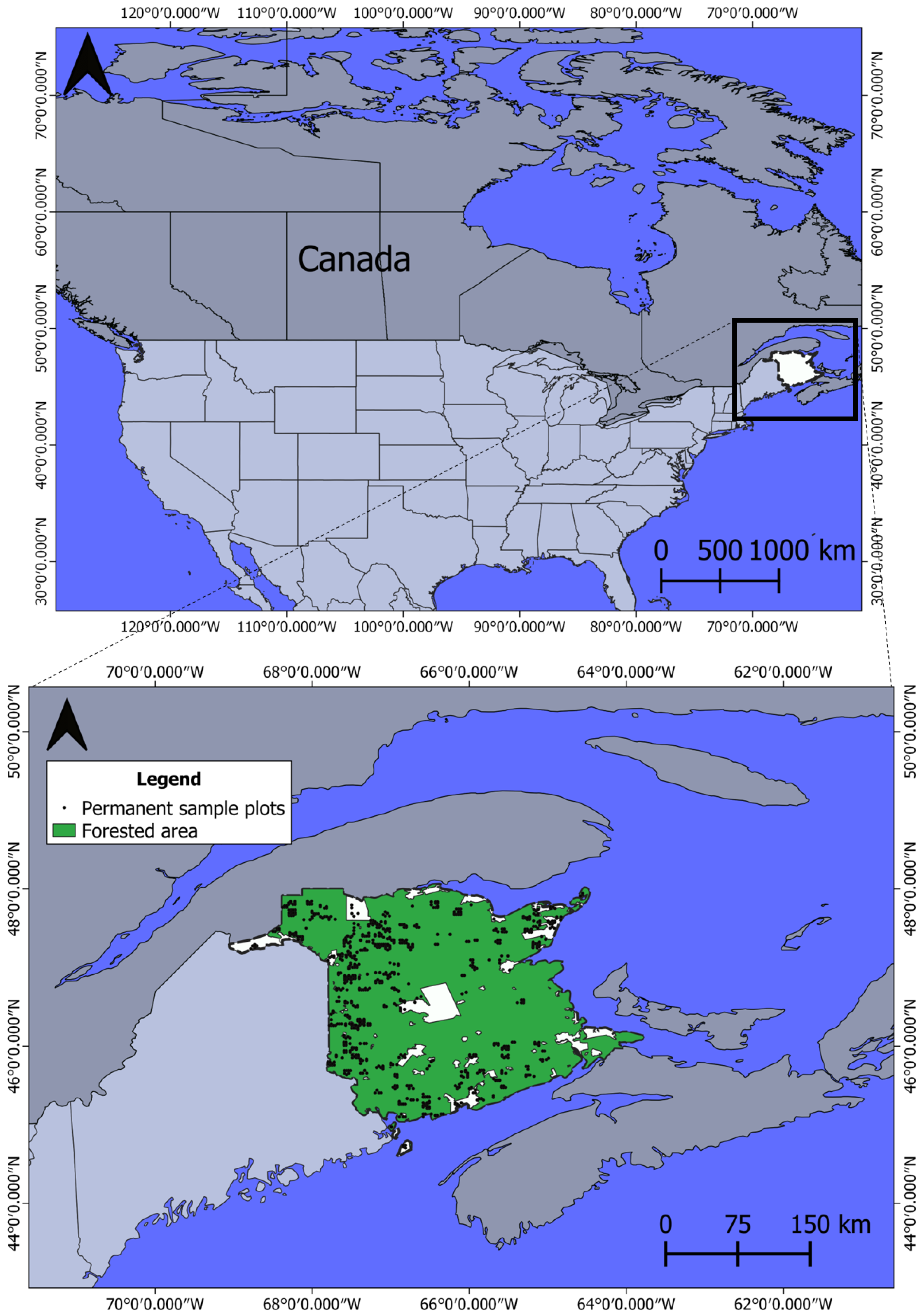
2.1. Study Area

We sampled forest stands across the entire province of New Brunswick in eastern Canada (66°21′42″ W, 46°31′05″ N, CRS: WGS84, Figure 1). This province is part of the Atlantic Maritime Ecozone, whose climate is strongly influenced by the Atlantic Ocean [48]. New Brunswick’s forest has been shaped by a long history of forestry. As a result, it is dominated by second- and third-growth stands, with small, scattered patches of old-growth [48]. Agriculture is restricted to valleys [49] and natural disturbances are dominated by eastern spruce budworm (Choristoneura fumiferana) outbreaks and fine-scale disturbances such as windthrows [50,51]. Most of New Brunswick’s forested lands are classified as Acadian forest, with a small portion of boreal forest in the northwestern corner of the province [52]. New Brunswick’s Acadian forest is characterized by a high species richness of both softwood and hardwood species, with spruces (Picea spp.), balsam fir (Abies balsamea), maples (Acer spp.), and birches (Betula spp.) as dominant canopy species [53].

2.2. Field Data

In this study, we used permanent sample plots (PSP) monitored by the New Brunswick Department of Natural Resources and Energy Development [54] and J.D. Irving Ltd. (n = 813). Almost all the PSP plots were distributed as a grid of 2 km × 2 km while the others were randomly distributed in stands of high values and intensively managed, 1/10th of the plots were measured annually.
Field surveys were performed ±1 year from the date of LiDAR coverage and Sentinel-2 image acquisition. We visually inspected each plot to ensure that no disturbance had taken place between the field survey and LiDAR capture. Because the annual growth in height of saplings is very variable due to different factors such as light intensity [55], initial height of the sapling [56], and shade-tolerance [57], we did not consider annual height growth of saplings as a bias in our study. Each stem with a diameter at breast height (DBH) of 1 to 7 cm and a height of ≥1.3 m was tallied in 50-m2 circular plots (3.99-m radius). Plot center location was determined with a GPS (Topcon HiPer SR, Topcon Corp., Tokyo, Japan) set up on a tripod. The tripod was placed in the center of the plot for a minimum of one hour to obtain high spatial accuracy (50 cm). For each stem tallied, species, DBH, and health class (live, dead, or declining) were recorded. Stem height was measured for every 10th stem using a clinometer.
All stems whose DBH was ≥7.1 cm were tallied in a 400-m2 circular plot (11.28-m radius) using the same plot center as for regeneration plots. Species, DBH, health class, and height were then recorded.

2.3. Satellite Images and Preprocessing

We used Sentinel-2 images with the highest resolution, 10 m × 10 m, acquired on 1 July 2016, 9 July 2017, and 21 July 2018. We used images from July to maximize our sample size (low cloud cover) and the highest image resolution to increase the accuracy of the models [33]. At this resolution, the images only include four bands: blue, green, red, and near-infrared (NIR). Since only level-1C images (top-of-atmosphere reflectance) were available for our study area, we performed an atmospheric correction using sen2cor plugin (SNAP software, ESA, Venice, Italy [58]). Then, we divided the digital number of each band by 10,000 to extract reflectance.
We only selected plots classified as vegetation from the scene classification generated by the sen2cor plugin for further analysis. Finally, for each plot, we extracted the mean reflectance of each band within an 11.28-m radius circle around the plot center and we calculated the normalized difference vegetation index (NDVI; Equation (1)). We selected NDVI because of its strong and well-described relation to canopy vegetation.
N D V I = N I R R e d N I R + R e d

2.4. LiDAR Acquisition and Preprocessing

LiDAR data were acquired during the summers of 2016, 2017, and 2018 using an aircraft mounted with a Riegl 680/780 (Riegl USA, Orlando, FL, USA) in 2016 and 2017, and a Riegl 1560 (Riegl USA, Orlando, FL, USA) in 2018. Each year, point density was set to 6 points/m2. The horizontal accuracy of point clouds for 2016 and 2017 was 30 cm, whereas it reached 20 cm in 2018. Vertical accuracy was 20 cm in 2016 and 2017 and 3 cm in 2018. The horizontal and vertical accuracy were similar to those of other studies aiming to characterize forest regeneration [25,38].
We only used returns classified as “ground” or “vegetation”. To do so, we first filtered points using LAStools software (rapidlasso GmbH, Gilching, Germany [59]) to remove those classified as building or noise, i.e., points not classified as “vegetation” or “ground”. Then, also with LAStools, we normalized vegetation points with ground points to calculate vegetation height above ground. Finally, we extracted points corresponding to field plots (11.28-m radius) and calculated LiDAR metrics for each plot using the lidR package (Roussel and Auty, Québec, Qc, Canada [60]) in the R statistical software (R Core Team, Vienna, Austria [61]) (Table 1).

2.5. Dependent Variables

We calculated the living stem density (stems/ha) of saplings for two species groups: (1) all species and (2) commercial species (Table 2). The “All species” group combined non-commercial and commercial species, whereas the other species group only comprised species having a commercial value. Both species groups included hardwood and softwood species (Table 2). On the other hand, all non-commercial species were hardwoods (Table 2). We defined a sapling as a stem whose DBH varied from 1 to 9 cm and whose height was ≥1.3 m.

2.6. Environmental Variables

We estimated canopy cover for each 11.28-m radius plot by calculating the proportion of all LiDAR points >7 m, which corresponds to the mean height of saplings in our study area. We also calculated the basal area of merchantable trees (DBH ≥ 9.1 cm), and the proportion of basal area of merchantable trees represented by hardwood species for each plot. We characterized plots using aspect, topography position index, and hillshade, which were derived from a digital elevation model (DEM) provided by the New Brunswick Department of Natural Resources and Energy Development (NBDNRED) at a resolution of 10 m. We also extracted ecoregion, ecodistrict, and ecosite [49], biomass growth index (BGI; [63]), depth to water table, soil type, and an index of the probability of occurrence of each species for every plot.

2.7. Statistical Analyses

To compare the accuracy of sapling density estimates between the different sensors (LiDAR, Sentinel-2 images, and both), we first built three models using random forest regression [64] for each dependent variable, i.e., absolute density of saplings of (1) all species and (2) commercial species. The first series of models combined variables from both sensors, LiDAR and Sentinel-2 images; the second series of models used LiDAR, whereas the third relied on Sentinel-2 images. In each model, environmental variables were also included.
We used the VSURF package [65] in R to select variables in each model based on their importance to reduce bias towards intercorrelated variables and categorical variables [66]. The model parameters entered were default values of ntree (500) and mtry (one-third of the variables), and we set the nodesize parameter to 1 to grow larger trees [64]. We then calculated the root means squared error (RMSE) with the randomForest package and obtained pseudo R-squared values for each model including only variables selected by the VSURF package. RMSE and pseudo R-squared values were calculated with internal values of mean squared error (MSE) and pseudo R-squared values of each tree (n = 500), respectively. We also computed relative RMSE (Equation (2)) and 95% confidence intervals (C.I.) of RMSE, relative RMSE, and pseudo R-squared to determine whether the accuracy and variance explained by the models differed.
R e l a t i v e   R M S E   ( % ) = R M S E 1 n i = 1 n A c t u a l × 100 .
Finally, to test the effect of canopy cover on the accuracy of each model, we performed a Kruskal–Wallis test on relative errors (Equation (3)) of four different intervals of canopy cover (low: 0% to 24%, medium: 25% to 49%, high: 50% to 74%, and very high: ≥75%). None of the transformations we tried could normalize the residuals from an ANOVA. Following significant Kruskal–Wallis tests, we performed a Dunn test using the Bonferroni correction to adjust p-values.
R e l a t i v e   e r r o r   ( % ) = P r e d i c t e d A c t u a l A c t u a l × 100 .

3. Results

3.1. Variable Selection and Model Accuracy

Contrary to our prediction, the integration of LiDAR and Sentinel-2 images did not increase the accuracy of sapling density estimates, nor it did for the variance explained compared to LiDAR for both species groups, i.e., all species combined and commercial species only (Table 3). Moreover, no spectral variables were retained in the models integrating the two sensors for both species groups (Table 3). However, the integration of both sensors, as for LiDAR, yielded higher accuracy and pseudo R-squared values compared to models using Sentinel-2 images for both species groups (Table 3).
When estimating sapling density for all species, the RMSE of the models combining both sensors or LiDAR only was similar (2828 no. stem/ha vs. 2836 no. stem/ha, respectively). For the model using Sentinel-2 images only, it was 3320 no. stem/ha (Table 3). When estimating sapling density for commercial species, the model integrating both sensors yielded an accuracy of 2784 no. stem/ha, and that using LiDAR only had a similar RMSE (2779 no. stem/ha) (Table 3). The model using Sentinel-2 images had an accuracy of 3165 no. stem/ha.
When estimating sapling density of all species, relative RMSE of the model combining both sensors and that using LiDAR was 84%, whereas it was 98% for the model using only Sentinel-2 images (Table 3). Therefore, relative RMSE of the model using Sentinel-2 images only was 14% higher than the model integrating both sensors and that using LiDAR. On the other hand, when estimating sapling density of commercial species, relative RMSE of the model integrating both sensors and that using LiDAR were identical at 100%, whereas relative RMSE of the model using Sentinel-2 images was 114% (Table 3). Again, relative RMSE of the model using Sentinel-2 images only was 14% higher than the model combining both sensors and that using LiDAR.
Pseudo R-squared of the models combining both sensors and those using LiDAR were similar at 0.33, when estimating sapling density of all species, and 0.23 and 0.24, respectively, when estimating sapling density of commercial species (Table 3). Pseudo R-square were lower for the models using Sentinel-2 images, at 0.08 when estimating sapling density of all species and 0.01 when estimating sapling density of commercial species (Table 3). When estimating sapling density of all the species, pseudo R-squared of the model using Sentinel-2 images was 25% lower than the model combining both sensors and the one using LiDAR. Furthermore, when estimating sapling density of commercial species, pseudo R-squared was 22% lower than the model integrating both sensors and 23% lower than the one using LiDAR.
In addition, 95% confidence intervals of RMSE, relative RMSE, and pseudo R-squared were similar between the models combining both sensors and those using only LiDAR for both species groups (Table 3). However, 95% confidence intervals of the models using Sentinel-2 images were larger from the ones of the models combining both sensors as well as from that of the models using LiDAR only, again for both species groups (Table 3). Those results are suggesting that the accuracy and the variance explained of the models integrating both sensors and the ones using LiDAR only did not differ statistically. To the contrary, models using Sentinel-2 images yielded significantly lower accuracy and variance explained than those combining both sensors or using LiDAR only.
As shown in Table 3, spectral variables were only selected in the model using Sentinel-2 images when species needed to be differentiated, thus estimating sapling density of commercial species, whereas only an environmental variable, basal area of tree with DBH ≥ 10 cm, was retained when estimating sapling density for all species.
On the other hand, some variables were retained in almost all models, irrespective of the species group considered. Those variables were the higher percentiles of LiDAR height distribution (zq75, zq80, and zq85), the proportion of LiDAR points near the ground (zpcum1), the percentage of LiDAR points >2 m (pzabove2), as well as the percentage of LiDAR points above LiDAR mean height (pzabovezmean; Table 3). For models combining both sensors, predicted values of sapling density for both species groups were higher when values of the highest percentiles of height distribution, the proportion of LiDAR points near ground, as well as above the mean height were low. In contrast, predicted values increased with the proportion of LiDAR points above 2 m (Figure 2 and Figure 3). These relations are indicating a denser vegetation in the lower than in the higher strata.

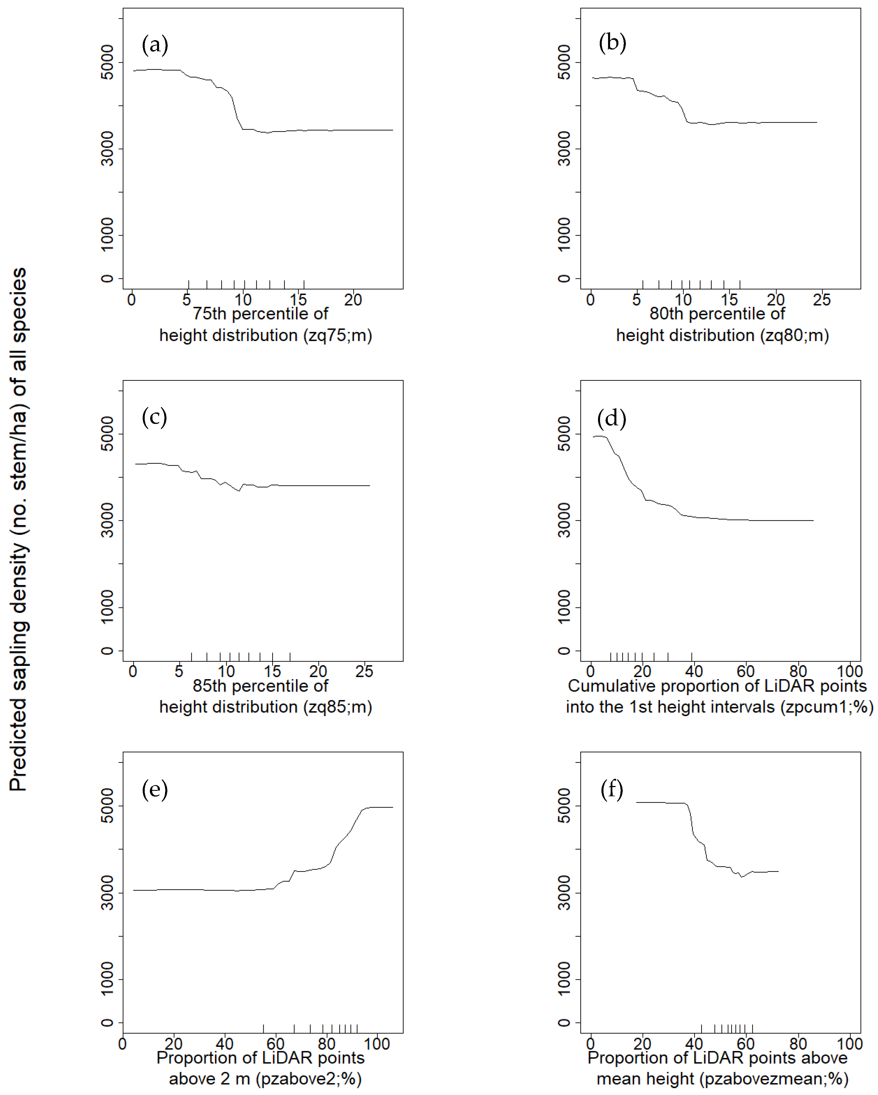
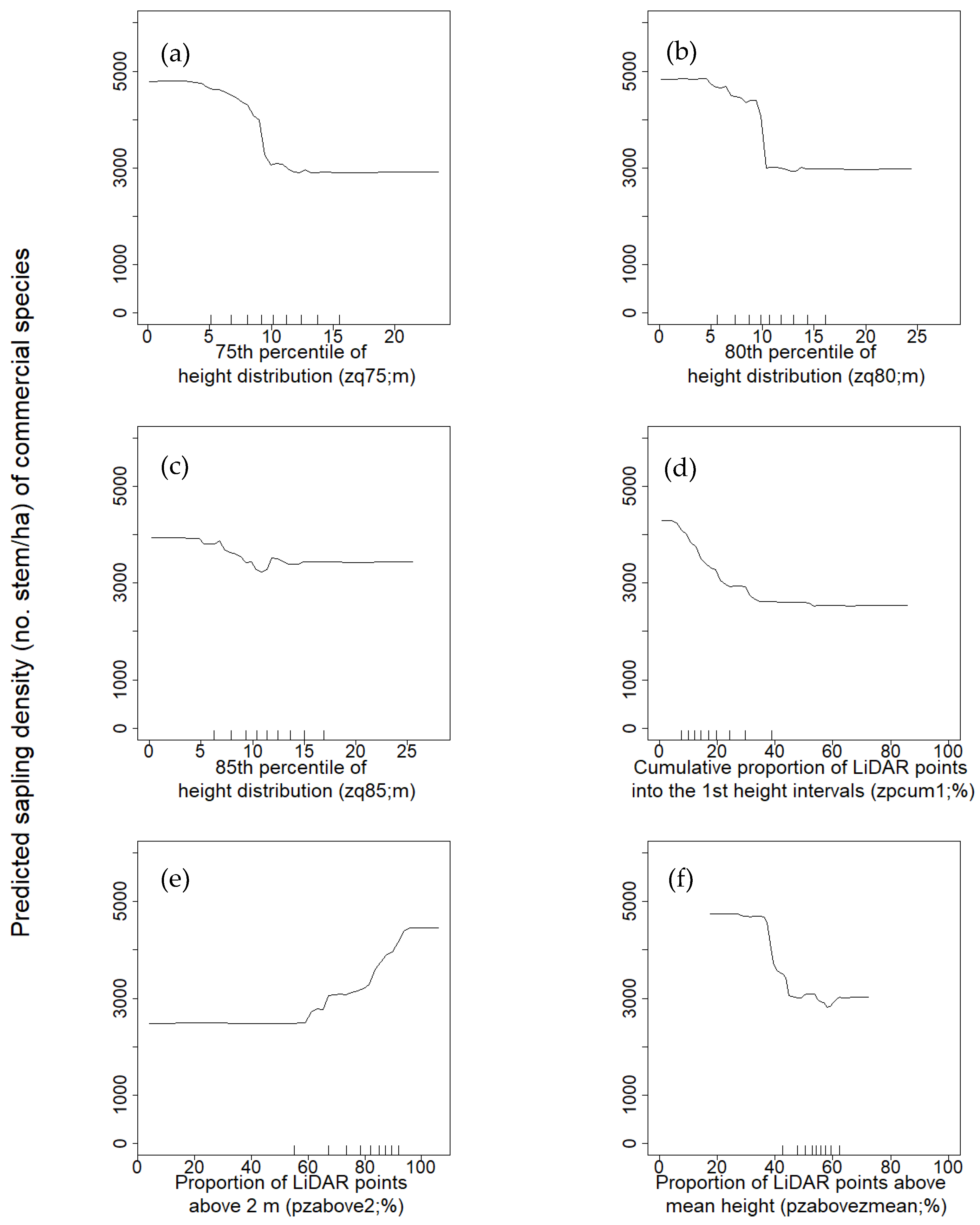
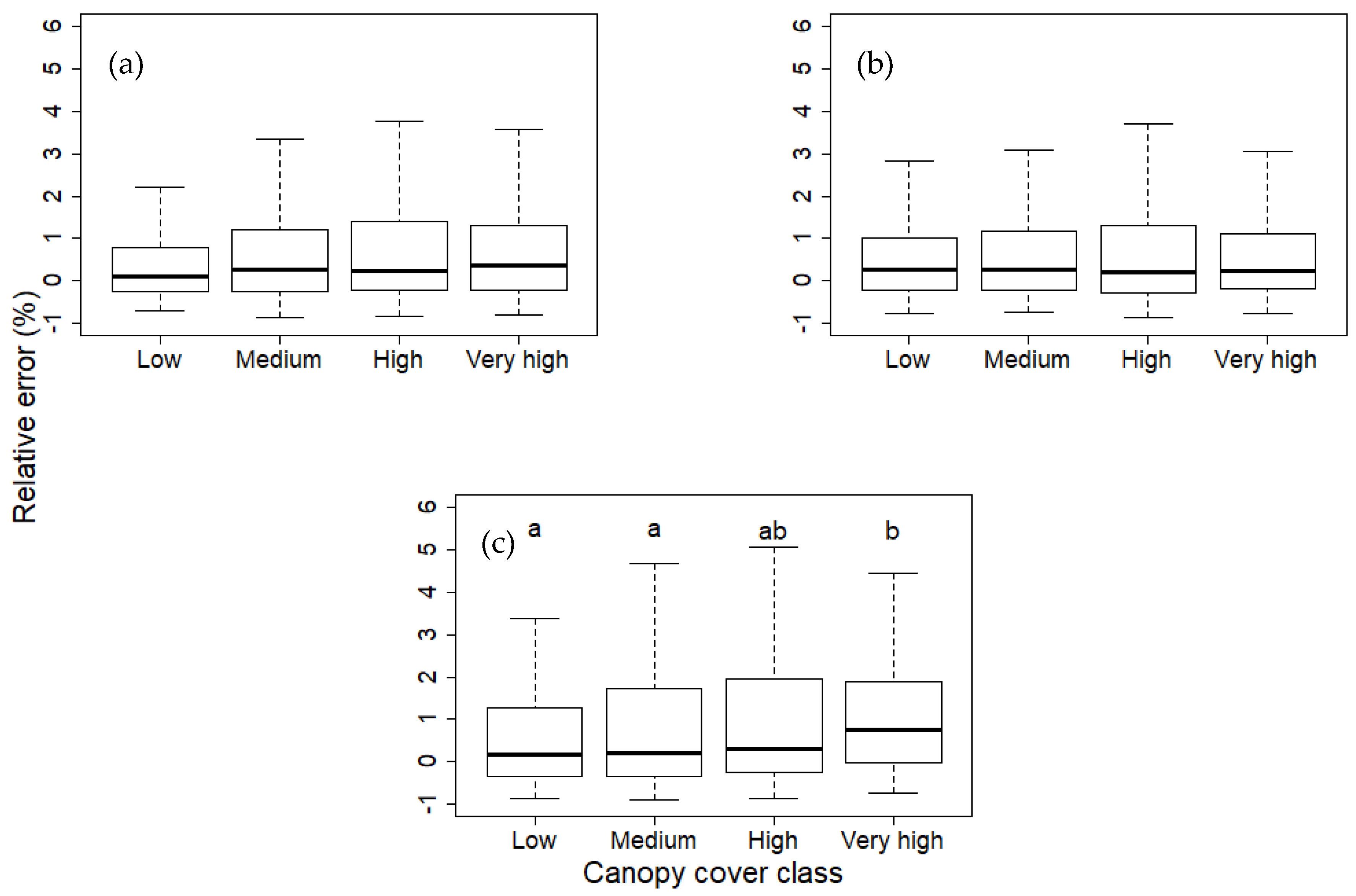
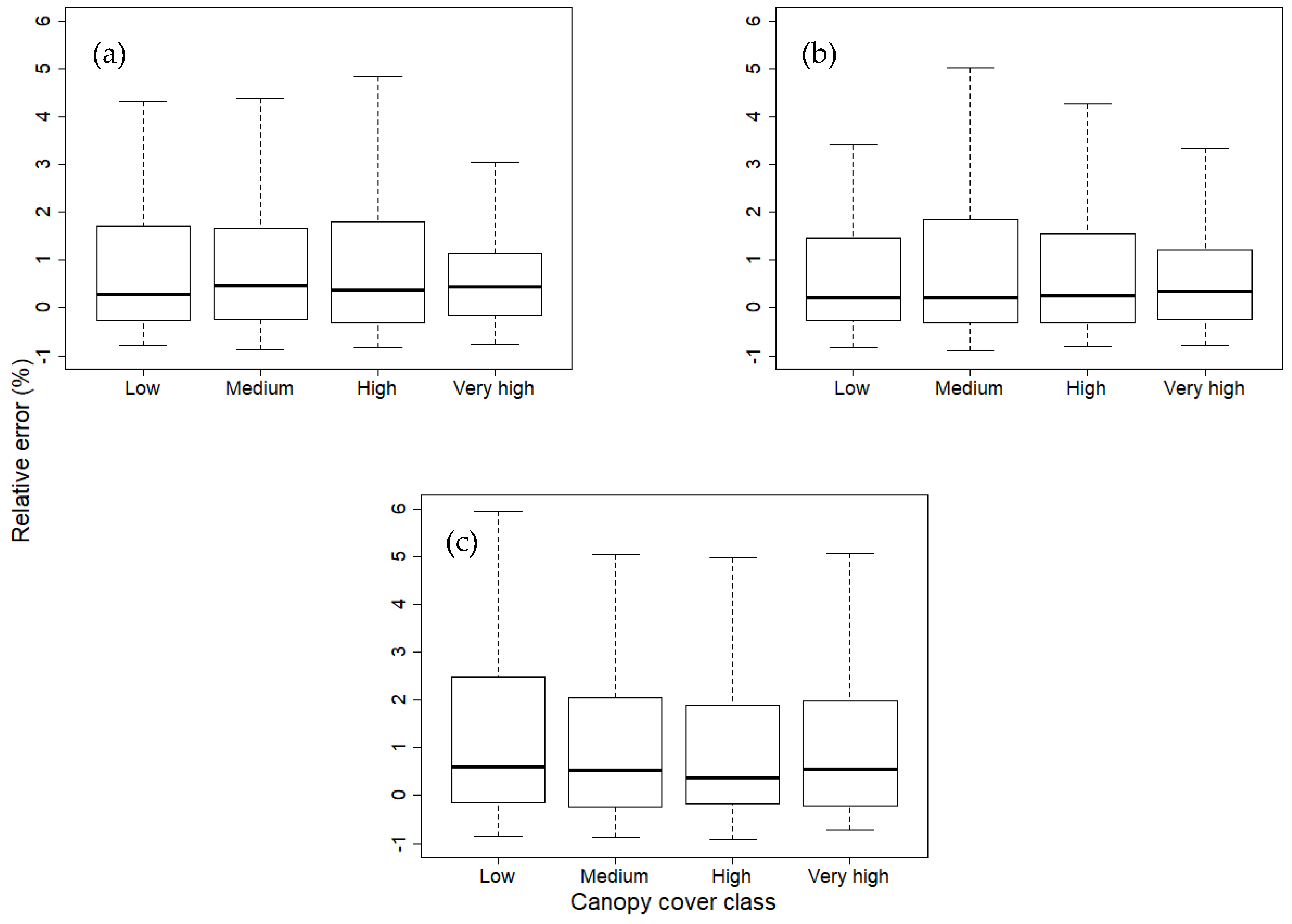
3.2. Effect of Canopy Cover

Models using LiDAR and those integrating both sensors had similar relative errors, irrespective of canopy cover class or species group considered ( Figure 4a,b and Figure 5a,b). By contrast and as predicted, the relative errors of sapling density estimates of both species groups increased under a very high canopy cover when using Sentinel-2 images along with environmental variables (Figure 4c and Figure 5c), although the difference was only significant when considering all sapling species (Figure 4c).

4. Discussion

4.1. Variable Selection and Model Accuracy

The combination of Sentinel-2 images and LiDAR did not increase the accuracy and variance explained for sapling density estimates of either species group (all species or commercial species) compared to LiDAR. Furthermore, no spectral variables were retained in the models integrating both sensors for either of the species groups. However, Leckie et al. [45] and Coops et al. [46] found that a combination of high-resolution (50 cm) images and LiDAR provided more accurate delineations of tree crowns. Pouliot et al. [33] also found that the accuracy of crown diameter estimates of planted seedlings increased with image resolution. Here, we used medium-resolution images (10 m) integrated with high-density LiDAR (6 points/m2). Perhaps high-resolution images would have increased the accuracy of sapling density estimates.
The integration of both sensors and the use of LiDAR yielded higher accuracy and variance explained compared to Sentinel-2 images. Other authors have also reported that LiDAR was more accurate than satellite images to estimate density [67], biomass [47], forest height [68], and basal area [41] of canopy trees in conifer and mixed stands. LiDAR is known to penetrate deeper into the canopy than satellite images [40].
Spectral variables were only selected in the model estimating sapling density of commercial species using Sentinel-2 images, whereas none were selected when estimating sapling density of all species. Commercial species included both softwoods and hardwoods species, whereas non-commercial species only comprise hardwoods species. This suggests that Sentinel-2 images helped to discriminate between hardwood species of commercial and non-commercial species. Satellite images have been shown to be more accurate than LiDAR to differentiate species [44]. Consistent with our results, the model integrating LiDAR and aerial images developed by Korhonen et al. [69] to estimate sapling density of all species also did not include any spectral variable. Here, we used images captured in summer. Key et al. [70] have shown that fall images are the best to identify species owing to their maximally contrasting spectral signatures. Hence, future studies should examine whether fall images could increase the accuracy of sapling density estimates.
We identified good predictors of sapling density, namely, the higher percentiles of height distribution (zq75, zq80, and zq85), and the proportion of LiDAR points between 2 m and the mean height of LiDAR points. A low value of the highest percentiles of height distribution indicates that the height of most of the vegetation is low, thus corresponding to saplings. Height distribution variables have also been shown elsewhere to be important to estimate stem densities >1 m [34,37,38]. Our results indicated a high density of saplings when the proportion of points near the ground (zpcum1) and above mean height (pzabovezmean) were low as well as when the proportion of points above 2 m (pzabove2) was high. Hence, we concluded that the proportion of points between 2 m and mean height was a good predictor of sapling density and that a high proportion of points between 2 m and mean height suggested a high density of saplings.

4.2. Effects of Canopy Cover

The integration of LiDAR and Sentinel-2 images also did not decrease the influence of canopy cover on the accuracy of sapling density estimates compared to LiDAR for both species groups. However, the accuracy of sapling density estimates of all species was significantly lower under a very high canopy cover when using Sentinel-2 images only. Donoghue and Watt [63] also found that under a closed canopy, a model using only LiDAR yielded accurate estimates of tree height. Indeed, satellite images are more sensitive to foliage characteristics than to tree height [41].

5. Conclusions

The integration of two sensors, LiDAR and Sentinel-2 images, did not outperform LiDAR when estimating sapling density, but it increased the accuracy of estimates compared to Sentinel-2 images. We identified two valuable predictors of sapling density: (1) the higher percentiles of height distribution (zq75, zq80, and zq85), and (2) the percentage of LiDAR points between a height of 2 m and mean height of LiDAR points. The influence of canopy cover on the accuracy of estimates was similar whether we used LiDAR or LiDAR and Sentinel-2 images combined. However, estimation accuracy was significantly lower under very high canopy covers (≥75%) when using Sentinel-2 images to estimate sapling density of all species. Hence, our results suggest that LiDAR alone is sufficient to estimate regeneration density in the Acadian forest across variable stand species compositions and canopy covers. Hence, when LiDAR is available, it should be prioritized over Sentinel-2 images. However, spectral variables were useful to differentiate species, and thus satellite images are highly recommended when information on sapling species composition is required. Finally, we recommend using the higher percentiles of height distribution (zq75, zq80, and zq85) and the proportion of LiDAR points between a height of 2 m and mean height of LiDAR points to obtain accurate estimates of sapling density in the Acadian forest under a range of canopy cover values.

Author Contributions

Conceptualization, G.P. and S.L.; formal analysis, S.L.; methodology, S.L. and G.P.; writing—original draft preparation, S.L.; writing—review and editing, M.-H.S.-L. and M.-A.V.; supervision, M.-H.S.-L., M.-A.V., and G.P. All authors have read and agreed to the published version of the manuscript.

Funding

This research was funded by the Northern Hardwoods Research Institute Inc.

Acknowledgments

We thank the province of New Brunswick and J.D. Irving Ltd. for providing the field data. Thanks to Chris Hennigar, Adam Dick, Pierre LeBel, and Elias Ayrey for their scientific advice and constructive comments, and to Peter Nelson and Kasey Legaard for their advice on pre-processing of Sentinel-2 images.

Conflicts of Interest

The authors declare no conflict of interest. The funder had a role as adviser in the design of the study, in the collection, analyses, and interpretation of data.

References

  1. Ashton, M.S.; Kelty, M.J. The Practice of Silviculture: Applied Forest Ecology, 10th ed.; John Wiley & Sons, Inc.: New York, NY, USA, 2018. [Google Scholar]
  2. Andersen, H.E.; Reutebuch, S.E.; McGaughey, R.J. A rigorous assessment of tree height measurements obtained using airborne lidar and conventional field methods. Can. J. Remote Sens. 2006, 32, 355–366. [Google Scholar] [CrossRef]
  3. Aplin, P. Remote sensing: Ecology. Prog. Phys. Geogr. 2005, 29, 104–113. [Google Scholar] [CrossRef]
  4. Means, J.E.; Acker, S.A.; Harding, D.J.; Blair, J.B.; Lefsky, M.A.; Cohen, W.B.; Harmon, M.E.; McKee, W.A. Use of large-footprint scanning airborne lidar to estimate forest stand characteristics in the Western Cascades of Oregon. Remote Sens. Environ. 1999, 67, 298–308. [Google Scholar] [CrossRef]
  5. Bergen, K.M.; Dronova, I. Observing succession on aspen-dominated landscapes using a remote sensing-ecosystem approach. Landsc. Ecol. 2007, 22, 1395–1410. [Google Scholar] [CrossRef]
  6. Franklin, S.E. Remote Sensing for Sustainable Forest Management; CRC Press: Boca Raton, FL, USA, 2001. [Google Scholar]
  7. Ogaya, R.; Barbeta, A.; Başnou, C.; Peñuelas, J. Satellite data as indicators of tree biomass growth and forest dieback in a Mediterranean holm oak forest. Ann. For. Sci. 2015, 72, 135–144. [Google Scholar] [CrossRef] [Green Version]
  8. Steininger, M.K. Satellite estimation of tropical secondary forest above-ground biomass: Data from Brazil and Bolivia. Int. J. Remote Sens. 2000, 21, 1139–1157. [Google Scholar] [CrossRef]
  9. Jaiswal, R.K.; Mukherjee, S.; Raju, K.D.; Saxena, R. Forest fire risk zone mapping from satellite imagery and GIS. Int. J. Appl. Earth Obs. 2002, 4, 1–10. [Google Scholar] [CrossRef]
  10. Hansen, M.C.; Loveland, T.R. A review of large area monitoring of land cover change using Landsat data. Remote Sens. Environ. 2012, 122, 66–74. [Google Scholar] [CrossRef]
  11. Simard, M.; Pinto, N.; Fisher, J.B.; Baccini, A. Mapping forest canopy height globally with spaceborne lidar. J. Geophys. Res. Biogeosci. 2011, 116. [Google Scholar] [CrossRef]
  12. Popescu, S.C.; Wynne, R.H.; Nelson, R.F. Measuring individual tree crown diameter with lidar and assessing its influence on estimating forest volume and biomass. Can. J. Remote Sens. 2003, 29, 564–577. [Google Scholar] [CrossRef]
  13. Coops, N.C.; Hilker, T.; Wulder, M.A.; St-Onge, B.; Newnham, G.; Siggins, A.; Trofymow, J.T. Estimating canopy structure of Douglas-fir forest stands from discrete-return LiDAR. Trees 2007, 21, 295. [Google Scholar] [CrossRef] [Green Version]
  14. Maltamo, M.; Mustonen, K.; Hyyppä, J.; Pitkänen, J.; Yu, X. The accuracy of estimating individual tree variables with airborne laser scanning in a boreal nature reserve. Can. J. For. Res. 2004, 34, 1791–1801. [Google Scholar] [CrossRef]
  15. Falkowski, M.J.; Smith, A.M.; Gessler, P.E.; Hudak, A.T.; Vierling, L.A.; Evans, J.S. The influence of conifer forest canopy cover on the accuracy of two individual tree measurement algorithms using lidar data. Can. J. Remote Sens. 2008, 34, S338–S350. [Google Scholar] [CrossRef]
  16. Latifi, H.; Heurich, M.; Hartig, F.; Müller, J.; Krzystek, P.; Jehl, H.; Dech, S. Estimating over-and understorey canopy density of temperate mixed stands by airborne LiDAR data. Forestry 2015, 89, 69–81. [Google Scholar] [CrossRef] [Green Version]
  17. Campbell, M.J.; Dennison, P.E.; Hudak, A.T.; Parham, L.M.; Butler, B.W. Quantifying understory vegetation density using small-footprint airborne lidar. Remote Sens. Environ. 2018, 215, 330–342. [Google Scholar] [CrossRef]
  18. Wing, B.M.; Ritchie, M.W.; Boston, K.; Cohen, W.B.; Gitelman, A.; Olsen, M.J. Prediction of understory vegetation cover with airborne lidar in an interior ponderosa pine forest. Remote Sens. Environ. 2012, 124, 730–741. [Google Scholar] [CrossRef]
  19. Næsset, E. Assessing sensor effects and effects of leaf-off and leaf-on canopy conditions on biophysical stand properties derived from small-footprint airborne laser data. Remote Sens. Environ. 2005, 98, 356–370. [Google Scholar] [CrossRef]
  20. Morsdorf, F.; Mårell, A.; Koetz, B.; Cassagne, N.; Pimont, F.; Rigolot, E.; Allgöwer, B. Discrimination of vegetation strata in a multi-layered Mediterranean forest ecosystem using height and intensity information derived from airborne laser scanning. Remote Sens. Environ. 2010, 114, 1403–1415. [Google Scholar] [CrossRef] [Green Version]
  21. Moskal, L.M.; Price, J.P.; Jakubauskas, M.E.; Martinko, E.A. Comparison of hyperspectral AVIRIS and Landsat TM imagery for estimating burn site pine seedling regeneration densities in the Central Plateau of Yellowstone National Park. In Proceedings of the Third International Conference on Geospatial Information in Agriculture and Forestry, Denver, CO, USA, 5–7 November 2001. [Google Scholar]
  22. Martín-Alcón, S.; Coll, L.; De Cáceres, M.; Guitart, L.; Cabré, M.; Just, A.; González-Olabarría, J.R. Combining aerial LiDAR and multispectral imagery to assess postfire regeneration types in a Mediterranean forest. Can. J. For. Res. 2015, 45, 856–866. [Google Scholar] [CrossRef]
  23. McCombs, J.W.; Roberts, S.D.; Evans, D.L. Influence of fusing lidar and multispectral imagery on remotely sensed estimates of stand density and mean tree height in a managed loblolly pine plantation. For. Sci. 2003, 49, 457–466. [Google Scholar]
  24. Korpela, I.; Tuomola, T.; Tokola, T.; Dahlin, B. Appraisal of seedling-stand vegetation with airborne imagery and discrete-return LiDAR–an exploratory analysis. Silva Fenn. 2008, 42, 753–772. [Google Scholar] [CrossRef] [Green Version]
  25. Su, J.G.; Bork, E.W. Integrating LIDAR data and multispectral imagery for enhanced classification of rangeland vegetation: A meta analysis. Remote Sens. Environ. 2007, 111, 11–24. [Google Scholar]
  26. Martinuzzi, S.; Vierling, L.A.; Gould, W.A.; Falkowski, M.J.; Evans, J.S.; Hudak, A.T.; Vierling, K.T. Mapping snags and understory shrubs for a LiDAR-based assessment of wildlife habitat suitability. Remote Sens. Environ. 2009, 113, 2533–2546. [Google Scholar] [CrossRef] [Green Version]
  27. Tuanmu, M.N.; Viña, A.; Bearer, S.; Xu, W.; Ouyang, Z.; Zhang, H.; Liu, J. Mapping understory vegetation using phenological characteristics derived from remotely sensed data. Remote Sens. Environ. 2010, 114, 1833–1844. [Google Scholar] [CrossRef]
  28. Hall, R.J.; Peddle, D.R.; Klita, D.L. Mapping conifer understory within boreal mixedwoods from Landsat TM satellite imagery and forest inventory information. For. Chron. 2000, 76, 887–902. [Google Scholar] [CrossRef] [Green Version]
  29. Chastain, R.A., Jr.; Townsend, P.A. Use of Landsat ETM and topographic data to characterize evergreen understory communities in Appalachian deciduous forests. Photogramm. Eng. Remote Sens. 2007, 73, 563–575. [Google Scholar] [CrossRef]
  30. Wang, T.; Skidmore, A.K.; Toxopeus, A.G.; Liu, X. Understory bamboo discrimination using a winter image. Photogramm. Eng. Remote Sens. 2009, 75, 37–47. [Google Scholar] [CrossRef] [Green Version]
  31. Fiorella, M.; Ripple, W.J. Determining successional stage of temperate coniferous forests with Landsat satellite data. Photogramm. Eng. Remote Sens. 1995, 59, 239–246. [Google Scholar]
  32. Potter, C.; Li, S.; Huang, S.; Crabtree, R.L. Analysis of sapling density regeneration in Yellowstone National Park with hyperspectral remote sensing data. Remote Sens. Environ. 2012, 121, 61–68. [Google Scholar] [CrossRef]
  33. Pouliot, D.A.; King, D.J.; Pitt, D.G. Development and evaluation of an automated tree detection delineation algorithm for monitoring regenerating coniferous forests. Can. J. For. Res. 2005, 35, 2332–2345. [Google Scholar] [CrossRef] [Green Version]
  34. Maltamo, M.; Packalén, P.; Yu, X.; Eerikäinen, K.; Hyyppä, J.; Pitkänen, J. Identifying and quantifying structural characteristics of heterogeneous boreal forests using laser scanner data. For. Ecol. Manag. 2005, 216, 41–50. [Google Scholar] [CrossRef]
  35. Hill, R.A.; Broughton, R.K. Mapping the understorey of deciduous woodland from leaf-on and leaf-off airborne LiDAR data: A case study in lowland Britain. ISPRS J. Photogramm. Remote Sens. 2009, 64, 223–233. [Google Scholar] [CrossRef]
  36. Sumnall, M.J.; Hill, R.A.; Hinsley, S.A. Comparison of small-footprint discrete return and full waveform airborne LiDAR data for estimating multiple forest variables. Remote Sens. Environ. 2016, 173, 214–223. [Google Scholar] [CrossRef] [Green Version]
  37. Korpela, I.; Hovi, A.; Morsdorf, F. Understory trees in airborne LiDAR data—Selective mapping due to transmission losses and echo-triggering mechanisms. Remote Sens. Environ. 2012, 119, 92–104. [Google Scholar] [CrossRef]
  38. Næsset, E.; Bjerknes, K.O. Estimating tree heights and number of stems in young forest stands using airborne laser scanner data. Remote Sens. Environ. 2001, 78, 328–340. [Google Scholar] [CrossRef]
  39. Wulder, M.A.; Franklin, S.E. Remote Sensing of Forest Environments; Springer: Boston, MA, USA, 2003; pp. 3–12. [Google Scholar]
  40. Pesonen, A.; Maltamo, M.; Eerikäinen, K.; Packalèn, P. Airborne laser scanning-based prediction of coarse woody debris volumes in a conservation area. For. Ecol. Manag. 2008, 255, 3288–3296. [Google Scholar] [CrossRef]
  41. Hudak, A.T.; Crookston, N.L.; Evans, J.S.; Falkowski, M.J.; Smith, A.M.; Gessler, P.E.; Morgan, P. Regression modeling and mapping of coniferous forest basal area and tree density from discrete-return lidar and multispectral satellite data. Can. J. Remote Sens. 2006, 32, 126–138. [Google Scholar] [CrossRef]
  42. Villikka, M.; Packalén, P.; Maltamo, M. The suitability of leaf-off airborne laser scanning data in an area-based forest inventory of coniferous and deciduous trees. Silva Fenn. 2012, 46, 99–110. [Google Scholar] [CrossRef] [Green Version]
  43. Imangholiloo, M.; Saarinen, N.; Markelin, L.; Rosnell, T.; Näsi, R.; Hakala, T.; Honkavaara, E.; Holopainen, M.; Hyyppä, J.; Vastaranta, M. Characterizing seedling stands using leaf-off and leaf-on photogrammetric point clouds and hyperspectral imagery acquired from unmanned aerial vehicle. Forests 2019, 10, 415. [Google Scholar] [CrossRef] [Green Version]
  44. Zald, H.S.; Ohmann, J.L.; Roberts, H.M.; Gregory, M.J.; Henderson, E.B.; McGaughey, R.J.; Braaten, J. Influence of lidar, Landsat imagery, disturbance history, plot location accuracy, and plot size on accuracy of imputation maps of forest composition and structure. Remote Sens. Environ. 2014, 143, 26–38. [Google Scholar] [CrossRef]
  45. Leckie, D.; Gougeon, F.; Hill, D.; Quinn, R.; Armstrong, L.; Shreenan, R. Combined high-density lidar and multispectral imagery for individual tree crown analysis. Can. J. Remote Sens. 2003, 29, 633–649. [Google Scholar] [CrossRef]
  46. Coops, N.C.; Wulder, M.A.; Culvenor, D.S.; St-Onge, B. Comparison of forest attributes extracted from fine spatial resolution multispectral and lidar data. Can. J. Remote Sens. 2004, 30, 855–866. [Google Scholar] [CrossRef]
  47. Hyde, P.; Dubayah, R.; Walker, W.; Blair, J.B.; Hofton, M.; Hunsaker, C. Mapping forest structure for wildlife habitat analysis using multi-sensor (LiDAR, SAR/InSAR, ETM+, Quickbird) synergy. Remote Sens. Environ. 2006, 102, 63–73. [Google Scholar] [CrossRef]
  48. Miller, R.F. Environmental History of the Atlantic Maritime Ecozone. In Assessment of Species Diversity in the Atlantic Maritime Ecozone; NRC Research Press: Ottawa, ON, Canada, 2010; pp. 13–303. [Google Scholar] [CrossRef]
  49. Zelazny, V.F.; Martin, G.L.; Toner, M.; Gorman, M.; Colpitts, M.; Veen, H.; Godin, B.; McInnis, B.; Steeves, C.; Wuest, L.; et al. Our Landscape Heritage: The Story of Ecological Land Classification in New Brunswick; New Brunswick Department of Natural Resources: Fredericton, NB, Canada, 2007.
  50. Mosseler, A.; Lynds, J.A.; Major, J.E. Old-growth forests of the Acadian Forest Region. Environ. Rev. 2003, 11, S47–S77. [Google Scholar] [CrossRef] [Green Version]
  51. Fraver, S.; White, A.S.; Seymour, R.S. Natural disturbance in an old-growth landscape of northern Maine, USA. J. Ecol. 2009, 97, 289–298. [Google Scholar] [CrossRef]
  52. Rowe, J.S. Forest Regions of Canada; Canadian Forestry Service: Ottawa, ON, Canada, 1972.
  53. Loo, J.; Ives, N. The Acadian forest: Historical condition and human impacts. For. Chron. 2003, 79, 462–474. [Google Scholar] [CrossRef]
  54. NBDNRED. Enhanced Forest Inventory Data Collection Protocols; New Brunswick Department of Natural Resources: Fredericton, NB, Canada, 2015.
  55. Petriţan, A.M.; von Lüpke, B.; Petriţan, I.C. Influence of light availability on growth, leaf morphology and plant architecture of beech (Fagus sylvatica L.), maple (Acer pseudoplatanus L.) and ash (Fraxinus excelsior L.) saplings. Eur. J. For. Res. 2009, 128, 61–74. [Google Scholar] [CrossRef] [Green Version]
  56. Claveau, Y.; Messier, C.; Comeau, P.G.; Coates, K.D. Growth and crown morphological responses of boreal conifer seedlings and saplings with contrasting shade tolerance to a gradient of light and height. Can. J. For. Res. 2002, 32, 458–468. [Google Scholar] [CrossRef] [Green Version]
  57. Janse-ten Klooster, S.H.; Thomas, E.J.P.; Sterck, F.J. Explaining interspecific differences in sapling growth and shade tolerance in temperate forests. J. Ecol. 2007, 95, 1250–1260. [Google Scholar] [CrossRef]
  58. Zuhlke, M.; Fomferra, N.; Brockmann, C.; Peters, M.; Veci, L.; Malik, J.; Regner, P. SNAP (sentinel application platform) and the ESA sentinel 3 toolbox. In Proceedings of the Sentinel-3 for Science Workshop, Venice, Italy, 2–5 June 2015. [Google Scholar]
  59. LAStools-Efficient Tools for LiDAR Processing. Version 141017. 2014. Available online: http://lastools.org (accessed on 7 May 2019).
  60. Roussel, J.-R.; Auty, D. lidR: Airborne LiDAR Data Manipulation and Visualization for Forestry Applications. 2017. Available online: https://cran.r-project.org/web/packages/lidR/index.html2017 (accessed on 12 June 2019).
  61. R Development Core Team. R Development Core Team R: A Language and Environment for Statistical Computing; R Foundation for Statistical Computing: Vienna, Austria, 2018. [Google Scholar]
  62. Woods, M.; Lim, K.; Treitz, P. Predicting forest stand variables from LIDAR data in the Great Lakes St. Lawrence Forest of Ontario. For. Chron. 2008, 84, 827–839. [Google Scholar] [CrossRef] [Green Version]
  63. Hennigar, C.; Weiskittel, A.; Allen, H.L.; MacLean, D.A. Development and evaluation of a biomass increment based index for site productivity. Can. J. For. Res. 2016, 47, 400–410. [Google Scholar] [CrossRef] [Green Version]
  64. Liaw, A.; Weiner, M. Classification and regression by randomForest. R News 2002, 2, 18–22. [Google Scholar]
  65. Genuer, R.; Poggi, J.M.; Tuleau-Malot, C. VSURF: An R package for variable selection using random forests. R J. 2015, 7, 19–33. [Google Scholar] [CrossRef] [Green Version]
  66. Strobl, C.; Boulesteix, A.L.; Zeileis, A.; Hothorn, T. Bias in random forest variable importance measures: Illustrations, sources and a solution. BMC Bioinform. 2007, 8, 25. [Google Scholar] [CrossRef] [PubMed] [Green Version]
  67. Pearse, G.D.; Dash, J.P.; Persson, H.J.; Watt, M.S. Comparison of high-density LiDAR and satellite photogrammetry for forest inventory. ISPRS J. Photogramm. Remote Sens. 2018, 142, 257–267. [Google Scholar] [CrossRef]
  68. Donoghue, D.N.M.; Watt, P.J. Using LiDAR to compare forest height estimates from IKONOS and Landsat ETM+ data in Sitka spruce plantation forests. Int. J. Remote Sens. 2006, 27, 2161–2175. [Google Scholar] [CrossRef]
  69. Korhonen, L.; Pippuri, I.; Packalén, P.; Heikkinen, V.; Maltamo, M.; Heikkilä, J. Detection of the need for seedling stand tending using high-resolution remote sensing data. Silva Fenn. 2013, 47, 1–20. [Google Scholar] [CrossRef] [Green Version]
  70. Key, T.; Warner, T.A.; McGraw, J.B.; Fajvan, M.A. A comparison of multispectral and multitemporal information in high spatial resolution imagery for classification of individual tree species in a temperate hardwood forest. Remote Sens. Environ. 2001, 75, 100–112. [Google Scholar] [CrossRef]
Figure 1. Location of the study area and distribution of permanent sample plots, which are scattered across the entire province of New Brunswick, Canada (CRS: WGS84).
Remotesensing 12 02440 g001
Figure 2. Partial dependence plots of (a) 75th (zq75), (b) 80th (zq80), and (c) 85th (zq85) percentiles of height distribution, (d) proportion of points in the first interval from ground (zpcum1), (e) proportion of LiDAR points above 2 m (pzabove2), and (f) proportion of LiDAR points above mean height (pzabovezmean; %) of random forest predictions of sapling density of all species (stems/ha) using both sensors.
Remotesensing 12 02440 g002
Figure 3. Partial dependence plots of (a) 75th (zq75), (b) 80th (zq80), and (c) 85th (zq85) percentiles of height distribution, (d) proportion of points in the first interval from ground (zpcum1), (e) proportion of LiDAR points above 2 m (pzabove2), and (f) proportion of LiDAR points above mean height (pzabovezmean; %) of random forest predictions of sapling density of commercial species (no. stem/ha) using both sensors.
Remotesensing 12 02440 g003
Figure 4. Distribution of the relative error (%; Equation (3)) as a function of canopy cover class (low: 0% to 24%, medium: 25% to 49%, high: 50% to 74%, and very high: ≥75%) for models estimating sapling density (stems/ha) of all species. (a) Model integrating both sensors, (b) model including LiDAR and environmental variables, and (c) model including spectral and environmental variables (Kruskal–Wallis test, (a) p = 0.30, (b) p = 0.92, and (c) p = 0.006). The groups a are statistically similar between them and different from group b, whereas group ab is statistically similar to group a and b.
Remotesensing 12 02440 g004
Figure 5. Distribution of the relative error (%; Equation (3)) as a function of canopy cover class (low: 0% to 24%, medium: 25% to 49%, high: 50% to 74%, and very high: ≥75%) for models estimating sapling density (stems/ha) of commercial species. (a) Model integrating both sensors, (b) model including LiDAR and environmental variables, and (c) model including spectral and environmental variables (Kruskal–Wallis test, (a) p = 0.85, (b) p = 0.99, and (c) p = 0.72).
Remotesensing 12 02440 g005
Table 1. Light Detection and Ranging (LiDAR) metrics used to estimate sapling density of all species and commercial species.
AbbreviationDescription
zmaxMaximum height
zmeanMean height
zsdStandard deviation of height distribution
zskewSkewness of height distribution
zkurtKurtosis of height distribution
zentropyEntropy of height distribution
pzabovezmeanPercentage of returns above zmean
pzabove2Percentage of returns above 2 m
zqxXth percentile of height distribution
zpcumxCumulative percentage of return in the xth layer according to Wood et al. [62]
itotSum of intensities for each return
imaxMaximum intensity
imeanMean intensity
isdStandard deviation of intensity
iskewStandard deviation of intensity
ikurtSkewness of intensity distribution
ipgroundPercentage of intensity returned by points classified as ground
ipcumzqxPercentage of intensity returned below the xth percentile of height
pxthPercentage xth returns
pgroundPercentage of returns classified as ground
Table 2. Species groupings for which sapling density was calculated.
Species GroupingSpecies
Commercial speciesHardwoodsAmerican beech (Fagus grandifolia)
American elm (Ulmus americanus)
Balsam poplar (Populus balsamifera)
American basswood (Tilia americana)
Black ash (Fraxinus nigra)
Black cherry (Prunus serotina)
Butternut (Juglans cinerea)
Green ash (Fraxinus pennsylvanica)
Grey birch (Betula populifolia)
Ironwood (Ostrya virginiana)
Large-tooth aspen (Populus grandidentata)
Oaks (Quercus spp.)
Red maple (Acer rubrum)
Silver maple (Acer saccharinum)
Sugar maple (Acer saccharum)
Trembling aspen (Populus tremuloides)
White ash (Fraxinus americanus)
White birch (Betula papyrifera)
Yellow birch (Betula alleghaniensis)
SoftwoodsBalsam fir (Abies balsamea)
Black spruce (Picea mariana)
Eastern hemlock (Tsuga canadensis)
Eastern White Cedar (Thuja occidentalis)
Jack pine (Pinus banksiana)
Norway spruce (Picea abies)
Red pine (Pinus resinosa)
Red spruce (Picea rubens)
Tamarack (Larix laricina)
White pine (Pinus stobus)
White spruce (Picea glauca)
Non-CommercialHardwoodsAmerican mountain ash (Sorbus americana)
Apple (Malus spp.)
Choke cherry (Prunus virginiana)
Hawthorns (Crataegus spp.)
Mountain maple (Acer spicatum)
Pin cherry (Prunus pensylvanica)
Serviceberry (Amelanchier spp.)
Speckled alder (Alnus rugosa)
Striped maple (Acer pensylvanicum)
Willows (Salix spp.)
Table 3. Variables selected and comparison of root means squared error (RMSE) (stems/ha), relative RMSE (%), and pseudo R-squared of models estimating sapling density of all species and commercial species using LiDAR metrics and/or spectral variables and environmental variables. See Table 2 for meaning of variable codes.
Candidate ModelsVariables SelectedRMSE (no. stem/ha; 95% C.I.)Relative RMSE (%; 95% C.I.)Pseudo R-Squared (95% C.I.)
Sapling density of all species
LiDAR + Spectral + Environmentalzq80 + zq75 + zq85 + zq60 + zq70 + zq55 + zq50 + zq40 + pzabove2 + zpcum1 + zq30 + zskew + pzabovemean + canopy cover + p1th + basal area 2828 (2814–2841)84 (84–84)0.33 (0.32–0.34)
LiDAR + Environmentalzq80 + zq85 + zq75 + zq70 + zq60 + zpcum1 + zq95 + zq55 + pzabove2 + zq30 + zq50 + pzabovezmean + basal area2836 (2827–2844)84 (84–84)0.33 (0.32–0.33)
Spectral + EnvironmentalBasal area 3320 (3317–3323)98 (98–98)0.08 (0.08–0.08)
Sapling density of commercial species
LiDAR + Spectral + Environmentalzq80 + zpcum1 + zq85 + zq75 + zq90 + pzabove2 + zq30 + zq95 + zq65 + zq60 + zpcum2 + zmean + zq50 +pzabovezmean2784 (2776–2792)100 (100–100)0.23 (0.23–0.24)
LiDAR + Environmentalzq80 + zq75 + zq85 + zpcum1 + zq90 + pzabove2 + zq70 + zq30 + zq60 + zpcum2 + zq50 + pzabovezmean2779 (2773–2785)100 (100–100)0.24 (0.23–0.24)
Spectral + EnvironmentalCanopy cover + basal area + proportion of hardwood + NDVI + Red + Blue + Green + Ecodistrict 3165 (3156–3174)114 (113–114)0.01 (0.002–0.01)

