Feasibility of Using the Two-Source Energy Balance Model (TSEB) with Sentinel-2 and Sentinel-3 Images to Analyze the Spatio-Temporal Variability of Vine Water Status in a Vineyard

Abstract

In viticulture, detailed spatial information about actual evapotranspiration (ET_a) and vine water status within a vineyard may be of particular utility when applying site-specific, precision irrigation management. Over recent decades, extensive research has been carried out in the use of remote sensing energy balance models to estimate and monitor ET_a at the field level. However, one of the major limitations remains the coarse spatial resolution in the thermal infrared (TIR) domain. In this context, the recent advent of the Sentinel missions of the European Space Agency (ESA) has greatly improved the possibility of monitoring crop parameters and estimating ET_a at higher temporal and spatial resolutions. In order to bridge the gap between the coarse-resolution Sentinel-3 thermal and the fine-resolution Sentinel-2 shortwave data, sharpening techniques have been used to downscale the Sentinel-3 land surface temperature (LST) from 1 km to 20 m. However, the accurate estimates of high-resolution LST through sharpening techniques are still unclear, particularly when intended to be used for detecting crop water stress. The goal of this study was to assess the feasibility of the two-source energy balance model (TSEB) using sharpened LST images from Sentinel-2 and Sentinel-3 (TSEB-PT_S2+3) to estimate the spatio-temporal variability of actual transpiration (T) and water stress in a vineyard. T and crop water stress index (CWSI) estimates were evaluated against a vine water consumption model and regressed with in situ stem water potential (Ψ_stem). Two different TSEB approaches, using very high-resolution airborne thermal imagery, were also included in the analysis as benchmarks for TSEB-PT_S2+3. One of them uses aggregated TIR data at the vine+inter-row level (TSEB-PT_airb), while the other is based on a contextual method that directly, although separately, retrieves soil and canopy temperatures (TSEB-2T). The results obtained demonstrated that when comparing airborne T_rad and sharpened S2+3 LST, the latter tend to be underestimated. This complicates the use of TSEB-PT_S2+3 to detect crop water stress. TSEB-2T appeared to outperform all the other methods. This was shown by a higher R² and slightly lower RMSD when compared with modelled T. In addition, regressions between T and CWSI-2T with Ψ_stem also produced the highest R².

1. Introduction

In a scenario of climate change and water scarcity, viticulturists will have to rely more on efficient irrigation management and adopting regulated deficit irrigation (RDI) strategies for successful grape production and wine quality [1,2,3,4]. To achieve these targets, accurate estimates of actual evapotranspiration (ET_a) and water status at the sub-field scale are necessary, particularly for specialty crops. Water requirements within a vineyard are variable due to differences in soil components [5,6,7] and administering uniform irrigation may result in either the over- or under-watering of some areas within the vineyard. Obtaining detailed spatial information about ET_a and vine water status within a given vineyard may therefore be of particular interest, particularly for applying site-specific, precision irrigation management.

Over recent decades, remote sensing techniques have been widely used for mapping and monitoring ET_a at the field scale, using satellite and airborne imagery. Several satellites have been used to estimate ET_a based on thermal infrared (TIR) data, whose spatial and temporal resolutions may vary [8]. Satellites such as Landsat (60-120 m), MODerate resolution Imaging Spectrometer (MODIS) (1 km), ASTER (90 m) and GOES (4 km) have been widely applied for mapping ET_a in irrigated agricultural fields [9,10,11,12]. Although extensive research has been carried out on ET_a estimates made with satellites, one of the major limitations of this approach is the coarse spatial resolution of satellite TIR images. In this context, the recent advent of Sentinel-2 and Sentinel-3 missions from the European Space Agency (ESA), as part of the Copernicus program (http://www.copernicus.eu/), has greatly improved the possibilities of monitoring crop parameters and estimating ET_a at higher temporal and spatial resolutions. Although Sentinel-3 carries a TIR sensor with a coarse spatial resolution of 1000 m at nadir, several other techniques could be used to sharpen the lower spatial resolution TIR observations with higher spatial resolution visible and near-infrared (VISNIR) observations [13,14,15,16]. These techniques involve empirically relating TIR to VISNIR spectral signals within the same scene, at the coarse pixel resolution of the thermal band, and then applying this relationship to the fine pixel resolution VISNIR bands in order to produce sharpened thermal band imagery at the same, with high resolution [16]. Guzinski et al. [17] evaluated the feasibility of sharpening daily Sentinel-3 (SLSTR sensor ~1000 m TIR data) satellite data with Sentinel-2 MIS (20 m VISNIR data). They obtained an acceptable level of accuracy and improvements in the estimates of fluxes, with respect to low-resolution satellite data. However, since the sharpened high-resolution land surface temperature (LST) is estimated from statistical relations using optical data (e.g., the correlation between LST and the NIR band), low LST used to correspond with pixels with high biomass and vice versa. One inherent limitation is the need to detect crop water stress in cases in which crops, and particularly those with heterogeneous or complex canopies, are stressed but without provoking a reduction in their leaf biomass.

On the other hand, very high-resolution thermal imagery, usually acquired from unmanned aerial vehicles (UAVs) or manned aircrafts, can potentially provide the spatial resolutions required for precision irrigation applications. Most current applications mainly focus on detecting crop water status in various woody trees [18,19,20,21] or on scheduling irrigation based on estimates of leaf water potential (Ψ_L) [22]. This last study estimated Ψ_L from a crop water stress index (CWSI) using an empirical approach which consisted of developing a baseline by normalizing differences between the canopy (T_c) and air temperatures (T_a) based on evaporative demand (by means of the vapor pressure deficit) [23,24]. Other studies have also used very high-resolution thermal infrared and multispectral data from airborne platforms to map ET_a over a vineyard [25,26,27]. One of the main shortcomings associated with using very high-resolution imagery would, however, be the need to provide this information on a routine basis over relatively large regions, given the need to calibrate this by crop, phenology and weather conditions [28].

Many different surface energy balance models have been widely used to estimate consumptive water use from ET_a (SEBAL, [29,30,31]; METRIC, [32]; TSEB, [33]; ALEXI, [34]; DISALEXI, [35]; DTD, [36]; ETEML, [37]). However, precision irrigation should focus on crop water fluxes and hence models are required that have the ability to separate ET_a into its component parts: soil evaporation (E) and canopy transpiration (T). One such model is the two-source energy balance (TSEB) land surface scheme [33], which has proven be fairly robust for a wide range of landscape and weather conditions [38,39,40]. The performance of the TSEB with satellite data relies on accurate observations of directional radiometric land surface temperature (LST). Canopy (T_c) and soil (T_s) temperatures are then estimated in an iterative process in which it is first assumed that the green canopy (expressed as the fraction of LAI that is green, f_g) transpires at a potential rate, which is based on the Priestley–Taylor formulation [41] (TSEB-PT), and that after that, a step-wise reduction of canopy transpiration can be performed until realistic daytime fluxes for both soil and canopy values are retrieved.

While waiting for the launch of a high-resolution TIR mission with a high revisit time, and given the open data access policies of the Copernicus satellites, it would seem reasonable to think—at least a priori—that the use of the TSEB-PT approach with Sentinel data and the adoption of disaggregation methods for downscaling spatial resolution could offer the most feasible option for a routine way of assessing water status at serviceable spatial and temporal scales and be used for precision irrigation purposes on an operational basis.

This paper evaluates the use of TSEB-PT with sharpened LST images from Sentinel-2 and Sentinel-3 for supporting operational irrigation decision-making in a vineyard throughout a full growing season. It also evaluates the accuracy of ET_a and T estimates with respect to very high-resolution airborne imagery and in situ vine physiological measurements. To the best of our knowledge, no other study has benchmarked the feasibility of using this methodology in an operational setting or quantified the feasibility of using it to detect vines under water stress. Based on the previously mentioned studies, which pointed to a good level of agreement between CWSI and Ψ_L using very high-resolution airborne imagery and demonstrated its workability for scheduling irrigation, one hypothesis of this study focuses on whether the theoretically based CWSI—which is defined as one minus the ratio of T, over potential transpiration (T₀) [24]—calculated with Sentinel data could provide an appropriate approach for detecting differences in vine water status.

2. Materials and Methods

2.1. Retrieval of TSEB Approaches

This study first evaluated estimates of actual transpiration (T) obtained with the TSEB model. We did this using three different methodologies which all make use of land surface temperature (LST): (i) TSEB-PT_S2+3 (PT for Priestley–Taylor), which uses sharpened LST from Sentinel-2 and Sentinel-3; (ii) TSEB-PT_airb, which is similar to TSEB-PT_S2+3, but which obtains LST from very high-resolution airborne thermal imagery; and (iii) TSEB-2T, which is a contextual approach that directly uses T_c and T_s, obtained from very high-resolution thermal imagery. Due to the difficulty involved in validating ET_a and its separate components, owing to the lack of eddy covariance or sap flow sensors, a spatio-temporal assessment of both actual and potential transpiration (T and T₀ respectively) was conducted through a vine water consumption model. Secondly, we analyzed different methodologies used to obtain the crop water stress index (CWSI) and related the results to stem water potential (Ψ_stem) measurements. We also used maps showing the spatial distribution of the ET components to assess the accumulated water consumption of the whole vineyard.

2.2. Two-Source Energy Balance (TSEB) Model

The TSEB land surface energy balance scheme has the advantage that it partitions estimates of sensible heat fluxes into canopy and soil layers. These depend on soil and canopy temperatures (T_s and T_c, respectively). The approach is therefore able to estimate canopy transpiration and soil evaporation separately. TSEB is based on the resistance network of the Shuttleworth and Wallace (1985) energy combination model, which has also been used in this study for computing potential transpiration (T₀). For more information, the full Python code is available online (https://github.com/hectornieto/pyTSEB, last accessed 22.09.2019) and additional details of the model are provided by Nieto et al. [27], Norman et al. [33] and Kustas et al. [42].

2.3. Priestley-Taylor Iterative Retrieval, TSEB-PT

The PT approach is used when TSEB is run at a coarse resolution and it is not possible to separate temperatures from pure canopy (T_c) and bare soil (T_s) pixels. In such cases, the observed directional radiometric temperature, $T_{RAD}\left(\theta \right)$, is partitioned into soil and canopy temperature (T_s and T_c, respectively), based on the vegetation cover fraction at the thermal sensor view angle, $f_c\left(\theta \right)$:

$$\sigma T_{RAD}^4\left(\theta \right)=f_c\left(\theta \right)\sigma T_c^4+\left[1-f_c\left(\theta \right)\right]\sigma T_s^4$$

(1)

T_c and T_s are used to separately compute the surface energy budgets for the soil and canopy components

$$R_{NS}=H_S+L{E}_S+G$$

(2)

$$R_{NC}=H_C+L{E}_C$$

(3)

$$H_S=\rho c_p\left(T_S-T_{ac}\right)/r_S$$

(4)

$$H_C=\rho c_p\left(T_C-T_{ac}\right)/r_X$$

(5)

where $R_{NS}$ is the net radiation at the soil surface; $R_{NC}$ is the net radiation in the canopy layer; $L{E}_S$ is the soil evaporation rate; $L{E}_C$ is the canopy transpiration rate; G is the soil heat flux; and $H_S$ and $H_C$ are the soil and canopy sensible heat fluxes (Equations (4) and (5)), which are directly related to T_s and T_c, respectively. ρ is the air density; c_p is the heat capacity of the air; T_ac is the aerodynamic temperature, or the air temperature at the sink–source height; and r_s and r_x are, respectively, the bulk canopy and soil resistances to heat transport.

In order to derive T_c and T_s from Equation (1), TSEB uses a first approximation of canopy latent heat flux, $L{E}_C$. This includes a first guess of canopy transpiration at the potential rates retrieved from the Priestley and Taylor model [33] (Equations (4) and (5)):

$$L{E}_C={\alpha }_{PT }{f}_c\frac{∆}{∆+\gamma }{R}_{NC}$$

(6)

where ${\alpha }_{PT}$ is the Priestley–Taylor coefficient, which was initially set to 1.26 [43] but subsequently automatically reduced for stress conditions; $∆$ is the slope of the saturation vapor pressure vs. temperature; and $\gamma$ is the psychrometric constant. With this initial value of LEc, the other soil and canopy flux components are retrieved from Equations (2)–(5). However, given that plants may be water-limited, TSEB-PT iteratively reduces the canopy transpiration value until realistic fluxes are obtained (i.e., allowing for non-negative latent heat fluxes during daytime, [33]) by looping between Equations (1)–(5).

2.4. Data Sharpening Scheme

In this study, the PT approach was compared using LST obtained by sharpening Sentinel-2 and Sentinel-3 images (TSEB-PT_S2+3) and from very high-resolution airborne thermal images (TSEB-PT_airb). The data sharpening method used in this study was based on the data mining sharpener (DMS) introduced by Gao et al. [16] and used by Guzinski et al. [13,17] with Sentinel 2 and Sentinel 3 data. This approach was also used by the European Space Agency (ESA) to develop the evapotranspiration plugin for the Sentinel Application Platform (SNAP) (www.esa-sen4et.org). The methodology consists of improving the coarse spatial resolution in LST retrievals from Sentinel-3 by sharpening the thermal band imagery using shortwave multispectral data. In addition, a regression tree approach was used to relate LST to a suite of shortwave spectral reflectance and ancillary data (e.g., elevation, illumination), at a coarse resolution, and then to apply it to a fine (shortwave band) pixel resolution to produce sharpened thermal band imagery. In this study, Sentinel-3 LST was sharpened to 20 m using nine bands of Sentinel-2. More information about the approach and code used is available online (https://github.com/radosuav/pyDMS, last accessed: 22.09.2019).

2.5. Contextual TSEB (TSEB-2T)

If high-resolution thermal imagery is available, it is possible to obtain T_s and T_c directly, without the need to compute an initial canopy transpiration [27]. In this study, we obtained the average canopy and soil temperature for each 20 x 20 m grid (coinciding with pixels of Sentinel-2) from very high-resolution airborne thermal images acquired on three different dates. The selection of pure canopy vegetation and soil pixels was obtained using a supervised classification method that took advantage of the semi-automatic classification plugin (SCP) of QGIS (QGIS 2.18.22) [44]. More details of the TSEB-2T model can be found in [27].

2.6. Biophysical Parameters of the Vegetation and Ancillary Data

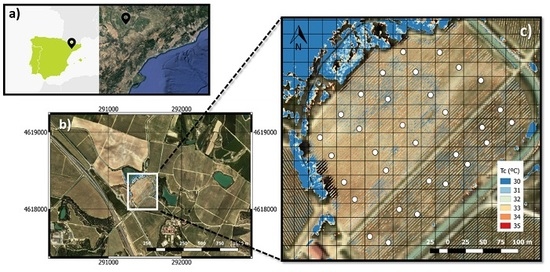
The biophysical parameters of the vegetation, such as its leaf area index (LAI) and the fraction of vegetation cover (f_c) used for running the TSEB and Shuttleworth and Wallace (S–W) models, were retrieved from atmospherically corrected Sentinel-2 reflectances with a spatial resolution of 20 m, and by using the biophysical processor available in the SNAP software v.6.0.1 [45]. This method creates a synthetic dataset of biophysical parameters covering the whole possible range of expected values; the reflectances of these pixels are then simulated using radiative transfer models (Prospect+SAIL, [46]) and convolved to the Sentinel-2 bands. Once these two datasets (of biophysical parameters and reflectances) have been generated, a neuronal network is built in order to predict the biophysical parameters from the Sentinel-2 band reflectances. The resulting estimates were used with the three methodologies tested (TSEB-PT_S2+3, TSEB-PT_airb and TSEB-2T). Other structural parameters of the vegetation, including its canopy height (h_c) and leaf width or canopy width to height ratio (w/h_c), were measured for the 32 vines that were distributed in the vineyard. Meteorological inputs were obtained from the local weather station, which was located 1 km from the study site [47].

2.7. Study Site

The study was conducted during the 2018 growing season, at a 6.6-ha vineyard of the Tempranillo grape variety, located at Raimat (Lleida, Spain) (41°41′19.40″ N; 0°29′37.16″ E, 280 m elevation) (Figure 1). The climate in the area is Mediterranean, and its average accumulated rainfall and reference evapotranspiration (ET_ref) during the growing season (1 April to 30 September) were 214 and 793 mm, respectively. The vines were 21 years old and were planted with a spacing of 1.6 × 2.5 m and a NE-SW row orientation. The vines were cordon-trained through a vertical shoot positioning (VSP) trellis system, with a bilateral, spur-pruned cordon located at a height of 0.9 m above the ground. The soil had a loamy texture, with an effective depth ranging from 0.6 to 1.2 m. The vines were drip-irrigated using drippers spaced 0.60 m apart along a single drip line per vine row. These lines discharged 4 l h⁻¹, with an irrigation frequency which varied from 2 to 3 days per week. The vineyard had a single irrigation sector and its irrigation scheduling was managed by the Raimat winery. The vine water requirements were calculated based on a water balance method to replace crop evapotranspiration (ET_c), in which ET_c was calculated from the ET_ref of Penman–Monteith [48] and crop coefficients derived from previous experiments [49,50], as follows: K_c1 = 0.2 (bud break on 5 April), K_c2 = 0.5 (bloom on 25 May to fruit-set on 5 June), K_c3 = 0.8 (mid-season, from veraison on 20 July until harvest) and K_c4 = 0.3 (at leaf fall at the end of October). During post-veraison, a regulated deficit irrigation (RDI) strategy was applied that consisted of reducing the amount of water administered by up to 50%. A water meter (CZ2000-3M Contazara, Zaragoza, Spain) was installed on the dripline to measure the volume of irrigation water applied. The total amount of water applied in the vineyard throughout the growing season was 280 mm. Disease control and vine nutrition management were conducted by the Raimat winery, following the protocols of the “Costers del Segre” Designation of Origin (Catalonia, Spain).

2.8. Satellite Data and Outputs of the TSEB model

A total of 28 Sentinel-2 and 44 Sentinel-3 cloud-free scenes were downloaded for the period 25 March to 15 October 2018 (

Table 1. Acquisition dates of the Sentinel 2 and Sentinel-3 cloud-free images used in the analysis (Sentinel 2: tile 31TBG, Sentinel 3: 6059) and airborne thermal imagery. For each Sentinel 2 acquisition, there is generally one or more Sentinel 3 acquisitions, with a maximum delay of 4 days relative to the Sentinel-2 acquisition date.

Sentinel-2 and Biophysical Parameters	Sentinel-3 and ET Products			Airborne
03-27-2018
04-01-2018
04-21-2018	04-24-2018
04-26-2018	04-27-2018
05-11-2018	05-13-2018
05-16-2018	05-16-2018	05-17-2018
05-31-2018	05-31-2018	06-01-2018
06-15-2018	06-16-2018
06-20-2018	06-20-2018	06-24-2018
06-25-2018	06-27-2018
06-30-2018	07-01-2018	07-02-2018
07-05-2018	07-05-2018	07-06-2018
07-10-2018	07-10-2018	07-14-2018
07-15-2018	07-17-2018	07-18-2018		07-18-2018
07-20-2018	07-24-2018
07-25-2018	07-25-2018	07-29-2018
07-30-2018	07-31-2018	08-01-2018	08-02-2018	07-31-2018
08-04-2018	08-05-2018	08-06-2018
08-09-2018
08-14-2018	08-17-2018
08-19-2018	08-20-2018	08-21-2018	08-22-2018	08-22-2018
	08-24-2018	08-29-2018	09-01-2018
	09-02-2018
09-08-2018	09-09-2018
09-13-2018	09-13-2018
09-18-2018
09-23-2018	09-24-2018	09-25-2018
09-28-2018	09-28-2018	09-29-2018
10-03-2018	10-03-2018	10-06-2018
10-08-2018	10-10-2018

). Sentinel-2 images were downloaded at level-1 (top of atmosphere reflectance) and atmospherically corrected using the Sen2Cor radiometric corrector [51]. These images were then resampled at 20 m in order to obtain the biophysical parameters of the vegetation. The land surface temperature (LST) was first obtained at the Sentinel-3 resolution, following the split-window approach proposed by Sobrino et al. [52]. Land surface energy fluxes and LST sharpening were derived for those days with available Sentinel-3 LST images that were within a 4-day difference of an S2 scene. The evapotranspiration components obtained were: actual evapotranspiration (ET_a); actual transpiration (T); soil evaporation (E); crop water stress index (CWSI), computed as one minus the ratio between the actual and potential transpiration; and the partitioning of the evapotranspiration expressed as the T/ET_a ratio. All the fluxes and metrics were integrated into daily values. To achieve this, the instantaneous latent flux estimates, expressed in W m⁻², were upscaled to daily water fluxes, expressed in units of mm/day, by multiplying the instantaneous ratio between the latent heat flux and solar irradiance by the average daily solar irradiance [53].

2.9. Shuttleworth-Wallace (S-W) Model and Crop Water Stress

In order to be consistent with TSEB, the two-layer Shuttleworth–Wallace (S–W) model [54] was used to estimate the potential evapotranspiration (ET₀) and to separate its component parts. The theoretical base of the S–W model is provided by the Penman–Monteith energy combination equation, which has two parts: one for the soil surface, and the other for the plant surface. The potential evapotranspiration and transpiration were computed with the S–W model by setting a minimum stomatal resistance value of 100 sm⁻¹. These values were then used as the base for estimating the theoretical CWSI.

The CWSI was then calculated as 1−T/T₀, using the Priestley–Taylor approach with sharpened S2+S3 LST (CWSI-PT_S2+3) and airborne imagery (CWSI-PT_airb) and applying the contextual approach (CWSI-2T).

In this study, CWSI was also computed using a baseline empirical approach (CWSI_e) [23]. This consisted of normalizing the difference between the air and canopy temperatures (T_c − T_a) using the vapor pressure deficit (VPD). In this study, the following baselines, developed by Bellvert et al. [55] for “Tempranillo” grapevines, were used to calculate the CWSI_e:

Lower limit: y = −1.780x + 1.253

(7)

Upper limit: y = 0.466x + 5.317

(8)

where y corresponds to T_c − T_a, and x represents VPD.

A seasonal spatio-temporal analysis was needed to better understand the feasibility of using this methodology throughout a whole growing season. However, due to the lack of available S2 and S3 data for certain days in the growing season (due to cloud cover), gaps had to be filled using daily continuous estimates of ET, which were obtained by calculating a crop water stress coefficient (K_s). K_s was calculated as the ratio between ET_a and ET₀, or as T/T₀, for those days with available satellite data. It was then extrapolated for those days within the same week with gaps in satellite data. This was achieved by multiplying the previously obtained value for K_s by the ET₀ or T₀ corresponding to dates with cloud cover.

2.10. Airborne Campaign

The airborne campaign consisted of three flights conducted on 18 (DOY 199) and 31 July (DOY 212) and 22 August (DOY 234) 2018. The vapor pressure deficits (VPD) and air temperatures (T_a) at the moment of image acquisition were 2.49 kPa and 29.9 ºC for DOY 199, 2.18 kPa and 31.2 ºC for DOY 212 and 2.51 kPa and 31.4 ºC for DOY 234. It is important to highlight that during the period from 12 to 17 August, there was a series of rainfall events at the study site which accounted for a total of 20 mm of precipitation. The aeroplane used was equipped with a thermal camera (FLIR SC655, FLIR Systems, Wilsonville, OR, USA) with a resolution of 640 x 480 pixels and a 13.1 mm focal length, with an FOV angle of 45°. The spectral response was in the range of 7.5–13 µm. The times of acquisition were between approximately 10:30 and 11:00 UTC (coordinated universal time), coinciding with the S3 satellite passing overhead. The plane flew over at a height of 180 m agl, capturing images with a resolution of 0.25 m pixels. At the beginning of each growing season, the thermal camera was radiometrically calibrated by the manufacturer (FLIR Systems s.r.l) using a very stable blackbody radiator. During the flight, in situ temperatures were acquired over homogeneous cold and hot targets, using a portable IR-gun (Fluke 572 infrared thermometer, Everett, WA, USA) in order to correct the atmospheric contribution to the signal. Image orthorectification and mosaicking were performed using off-the-shelf photogrammetric software. This was completed with the aid of ground control point (GCP) targets, after their geolocations on the ground had been collected with a handheld GPS (Global Positioning System) (Geo7x, Trimble GeoExplorer series, Sunnyvale, CA, USA).

2.11. Field Measurements

Physiological and structural measurements of the vines were conducted at a total of 32 points which were uniformly distributed across the vineyard. Each point related to three vines. Midday stem water potential (Ψ_stem) was measured for each vine (two measurements per point), using a pressure chamber (Soil Moisture plant water status console 3005 Corp. Sta. Barbara, CA, USA). To ensure a balance between the leaf and the stem attached to it, shaded leaves located near the main trunk were wrapped in plastic bags covered with aluminum foil for 1 h prior to taking the Ψ_stem measurements. All the measurements were taken in less than 1 hour, with their timing coinciding with that of the image acquisition on the airborne campaign days. The fraction of PAR light intercepted by the crop (fiPAR) and the LAI were determined as indicators of vegetative development, using a portable ceptometer (Accupar, Decagon Devices Inc., Pullman, WA, USA). Measurements were taken on each vine, using a 12-point grid that was measured at ground level and by covering the vine spacing distance. Incident radiation readings were measured above the vines. There was a total of seven measuring days, three of which coincided with the image acquisition dates. Daily fiPAR (fiPAR_d) was calculated using the hourly model for light interception [56] and by adjusting the porosity parameter in Oyarzun’s model so that the noon fiPAR value of the hourly simulation matched that measured in the field concomitant to where the image was acquired. Structural parameters such as vine height, and vine width, both perpendicular to and along rows, were also measured, using a ruler. Effective LAI was obtained from fiPAR, using the approach presented by Norman et al. [57] and setting a leaf absorptivity for light of 0.85.

2.12. Spatio-Temporal Validations with the Vine Water Consumption Model

The estimates of actual and potential transpiration obtained with the TSEB and S–W models throughout the growing season were compared with those generated by a vine water consumption crop model. This model has been developed for grapevines and successfully used for conducting precision irrigation scheduling at a commercial vineyard over two consecutive growing seasons. A full description of the model has been provided by Bellvert et al. [58]. Although this model is able to simulate evapotranspiration, in this study, we only used it for estimates of transpiration. The reason for this is that soil evaporation is related to the total size of the wet soil surface, and this depends on the timing of applying irrigation. Since water meter readings were taken manually, on a weekly basis, we did not have all the information required to accurately estimate the soil evaporation component. In situ measurements of the fraction of intercepted radiation (fiPAR) and the midday stem water potential (Ψ_stem) are required in order to obtain modelled values for T and T₀.

The spatio-temporal assessments of crop stress using the different methodologies (TSEB-PT_S2+3, TSEB-PT_airb and TSEB-2T) were conducted for 32 vines and on three different image acquisition dates (DOY 199, 212 and 234). In addition, the temporal evaluation of TSEB-PT_S2+3 was carried out at two representative extreme zones within the vineyard. This was done throughout the growing season and covered well-watered and stressed grapevines.

3. Results and Discussion

3.1. Spatial Assessment of Transpiration

Spatially distributed, remotely sensed estimates of actual and potential transpiration were obtained using three different methodologies and compared with those modelled using a vine water consumption model.

Table 2. Accuracy statistics for regressions between modelled transpiration, obtained from the vine water consumption model, and estimates of potential and actual transpiration. The latter were respectively estimated using: the Shuttleworth and Wallace model (T₀ S–W); two-source energy balance (TSEB) with (i) Priestley–Taylor with sharpened LST from Sentinel-2 and Sentinel-3 (T TSEB-PT_S2+3), (ii) PT with LST obtained from very high-resolution airborne thermal imagery resampled at 20 m (T TSEB-PT_airb) and (iii) the separation of canopy (T_c) and soil (T_s) temperatures obtained from very high-resolution airborne thermal imagery (T TSEB-2T), and correlations with the crop water stress index (CWSI), calculated as 1-T/T₀. CWSI_e represents the CWSI obtained with the empirical baseline approach for cv.Tempranillo, using the following equations: y = −1.780x + 1.253 and y = 0.466x + 5.317 (Bellvert et al. 2015), to establish the lower and upper limits. Root mean square deviation (RMSD) and bias (modelled without the estimated values) are expressed in mm day⁻¹; the coefficient of variation (C_V—RMSE divided by the mean of the modelled values), equation (estimated = a modelled + b) and coefficient of determination (R²) are unitless. Only statistically significant regressions between the remote sensing results and water consumption model are shown.

	DOY 199					DOY 212					DOY 234					All
	RMSD	Bias	CV	Equation	R2	RMSD	Bias	CV	Equation	R2	RMSD	Bias	CV	Equation	R2	RMSD	Bias	Cv	Equation	R2
T0 S-W	0.24	0.02	0.07	0.86x + 0.37	0.78	0.35	−0.09	0.10	1.12x − 0.26	0.74	0.44	−0.34	0.16	0.89x + 0.66	0.71	0.27	−0.06	0.12	0.95x + 0.17	0.73
T TSEB-PTS2+3	0.47	0.02	0.23	0.25x + 1.63	0.47	0.53	0.47	0.22	0.40x + 1.52	0.61	0.51	−0.23	0.21	0.44x + 1.51	0.55	0.49	0.07	0.21	0.38x + 1.51	0.48
T TSEB-PTairb	0.72	0.59	0.32	0.35x + 0.81	0.69	0.73	0.60	0.30	0.51x + 0.55	0.72	0.68	0.58	0.30	0.51x + 0.52	0.63	0.71	0.20	0.31	0.47x + 0.60	0.67
T TSEB-2T	0.41	0.26	0.18	0.53x + 0.74	0.82	0.50	0.27	0.18	0.59x + 0.52	0.77	0.43	0.23	0.19	0.55x + 0.80	0.65	0.49	0.33	0.22	0.55x + 0.70	0.72
CWSI-PTS2+3	0.13	0.00	0.43	-	-	0.18	0.09	0.90	-	-	0.07	0.01	0.22	0.27x + 0.23	0.43	0.15	0.01	0.52	0.25x + 0.19	0.18
CWSI-PTairb	0.20	−0.16	0.69	0.14x + 0.44	0.41	0.27	−0.22	1.34	0.15x + 0.41	0.32	0.18	−0.16	0.52	0.25x + 0.41	0.25	0.23	−0.19	0.84	0.18x + 0.42	0.36
CWSI-2T	0.11	−0.07	0.40	0.36x + 0.27	0.66	0.22	−0.18	1.08	0.31x + 0.32	0.57	0.11	−0.07	0.33	0.22x + 0.33	0.18	0.18	−0.06	0.63	0.28x + 0.31	0.47
CWSIe	0.11	−0.07	0.37	1.03x − 0.08	0.65	0.22	−0.19	1.05	1.37x − 0.34	0.71	0.15	0.08	0.46	-	-	0.17	−0.12	0.62	0.28x + 0.25	0.20

presents a summary of the statistics used to evaluate the performance of the different methods. It shows that estimates of T₀ obtained with the S–W model yielded results that closely agreed with the modelled T₀ values for all three dates and that when the data were analyzed together, R² ranged from 0.71 to 0.78. TSEB-2T also appeared to outperform all the other models, yielding closer agreement with modelled T. This was shown by the higher R² value and slightly lower root mean square deviation (RMSD) for the three measured dates and also by encompassing all the data together. This suggested that whenever it is possible to retrieve T_c and T_s directly from very high-resolution thermal imagery, the accuracy of the estimates of T could significantly improve in comparison with other tested methodologies. Although the transpiration derived from TSEB-PT_airb did not provide the same accuracy as fluxes derived from TSEB-2T, it provided improved values compared with TSEB-PT_S2+3. In addition to lower R² values, the latter also exhibited slopes that significantly differed from 1 in all cases, suggesting that this approach tends to overestimate low transpiration rates. We also noted that all three methodologies (TSEB-PT_S2+3, TSEB-PT_airb and TSEB-2T) tended to give slightly lower T values at rates higher than approximately 2.5 mm day⁻¹, with this bias being more pronounced for the two methods which used airborne thermal imagery. This could probably be explained as follows: i) in TSEB-2T, the average T_c for all the vines within the 20 x 20 m pixel (~20 vines) could have been higher than it should have been for the three measured vines due to either the selection of mixed pixels combining vegetation and soil or because of within-pixel spatial variability in water status; ii) as TSEB-PT_airb uses the Priestley–Taylor approach and this is based upon an initial guess that assumes that the vines transpire at their potential rate, it is essential to have a robust characterization of the canopy potential transpiration; and iii) bias is more pronounced in methods which use airborne thermal imagery (TSEB-2T and TSEB-PT_airb) than in TSEB-PT_S2+3 because the sharpened LST of the latter tends to be overestimated (Figure 2) and, as a consequence, the estimated T rates tend to be higher.

As with transpiration, the modelled CWSI also agreed with the values obtained using the contextual (CWSI-2T) method, although the closest agreement was obtained using the baseline empirical approach (CWSI_e) (Table 2). In both cases, the results were robust for DOY 199 and 212 with the RMSD and R² respectively ranging from 0.11 to 0.22 and from 0.57 to 0.71. When the data for all three dates were encompassed, CWSI-2T was also the approach with the highest R² and lowest RMSD values. However, DOY 234 showed only a low level of agreement for all the methodologies except CWSI-PT_S2+3. This was possibly due to the effect of the 20 mm of rainfall received in the week before the image was acquired. The effects of convective rainfall occurring a few days before image acquisition on the CWSI have been previously described by Bellvert et al. [22], who observed that rainfall may modify the VPD and air temperature within the vineyard as the amount of water evaporated from the soil and vegetation surfaces is high. In consequence, the evaporative demand within the vineyard may be lower than at the location where the meteorological data were gathered and this may affect the accuracy of estimates of CWSI. Another hypothesis was that T_s was clearly lower than for previous days due to the soil being wetter: this was detected by very high-resolution imagery. Partitioning readings into E and T would have probably tended to overestimate E and to underestimate T, thereby resulting in an overestimation of the CWSI values. The regressions obtained using the CWSI-PT_S2+3 method were not significant, with the partial exception of DOY 234 and when all three dates were plotted together. It seems that although the overall RMSD values were low, they tended to increase as the CWSI increased. This suggests that this approach was unable to detect severely water-stressed vines. On the other hand, the result for DOY 234 was significant, probably because of there being a lower degree of water stress, as apparently reflected by the smaller range in CWSI values associated with the rainfall event. In fact, Figure 2 shows the regression between LST with sharpened S2 and S3 and airborne LST, resampled at 20 m. This shows that estimates of high-resolution satellite LST obtained using the DMS approach tended to be underestimated, which tended to increase with higher LST values. The average RMSE values were 3.8 ºC, 3.1 ºC and 3.7 ºC, for DOY 199, 212 and 234, respectively. Figure 2b also shows that there was quite a strong correlation between RMSE and LST. This tended to increase as the LST values increased, with similar slopes for all three dates. In agreement with this, it is interesting to note that the LST values for DOY 234 were significantly lower than for the other two days. The good correlation between the sharpened and actual LST values shown in Figure 2b highlights the fact that sharpening the LST from 1 km to 20 m was able to resolve some of the spatial variability in surface temperature at the farm scale. However, its major underestimation shows that this sharpening was unable to capture the full range of temperatures registered under water-stressed conditions. This was probably due to the fact that the actual dynamic range of LST at 1 km was smaller than at 20 m and, in particular, when different rainfed and irrigated areas were present within the coarse-resolution pixel. The decision tree regression model was therefore trained using a set of temperatures with a narrower range than should normally be used to predict a larger range of temperatures.

3.2. Temporal Evaluation of T (TSEB-PT_S2+3) And T₀ in Well-Watered And Stressed Vines

Figure 3 illustrates the temporal evolution of T (TSEB-PT_S2+3) and T₀ (S-W) for well-watered (Figure 3a) and stressed vines (Figure 3b) in the vineyard. It also shows comparisons with values modelled based on the vine water consumption model. The figure also includes the seasonal evolution of LAI and FAPAR estimated from Sentinel-2 using the biophysical processor and the modelled values for daily fiPAR (fiPAR_d) and the measured value for Ψ_stem. Ψ_fc and Ψ_wilt respectively correspond to the stem water potential at field capacity and the lowest plant water potential at wilting point, when transpiration is null. Both these parameters are obtained from the vine water consumption model [58].

The well-watered vines must have been transpiring at near to full potential rates. This was shown by the small differences between T₀ and T throughout the growing season and by the fact that the Ψ_stem values were close to Ψ_fc (Figure 3a). The seasonal average RMSDs for T and T₀ were 0.46 and 0.64 mm day⁻¹, respectively. Transpiration tended to increase sharply from DOY 100 (beginning of April) to 160 (mid-June), when maximum values of 4.2 mm day⁻¹ for T₀ and 3.8 mm day⁻¹ for T were registered. After DOY 230 (mid-August), transpiration began to moderately decline until senescence. When we compared the modelled and estimated values of T and T₀ between well-watered and stressed vines, as expected, we found significantly lower rates for the latter throughout the growing season. Although the RMSD values for T and T₀ were similar, the seasonal averaged R² values of the stressed vines were significantly lower (Figure 3b). The T values of stressed vines were slightly overestimated throughout the growing season, although the largest differences with respect to the modelled T values were detected during the period of highest water stress (from DOY 180 to 240). Figure 3b.2 shows how the Ψ_stem values were lower during that particular period. This confirmed the hypothesis that the underestimation of sharpened satellite S2+3 LST for high LST values (Figure 2) would be reflected in an overestimation of T. Under both water regimes, the highest RMSD values were concentrated at the beginning and at the end of the growing season. This was probably because during these two periods, the cover cropping between rows tended to be higher and this was reflected in the higher estimates of satellite LAI. This was probably also linked to the fact that TSEB is only able to account for a single, actively transpiring canopy layer [59]. A similar consideration was reported by Semmens et al. [10]. Despite this, if we assume that most of the intercepted PAR was actually absorbed during the growing season, the R² between the estimates of FAPAR made with Sentinel-2 and the modelled fiPAR_d would have been 0.92. Few studies have validated Sentinel-2 FAPAR products in heterogeneous crops such as grapevines. Although the correlation obtained probably depended on the training system, spacing distance and/or row orientation, and further research will be needed to adapt FAPAR estimates to these conditions, the preliminary results seem promising.

3.3. Comparison Between Methodologies

Estimates of actual evapotranspiration (ET_a) and transpiration (T) obtained with TSEB-PT_S2+3 showed a significant level of correlation with other methodologies. R² values of 0.83 and 0.65 (ET_a) and of 0.78 and 0.70 (T) were obtained when they were compared with TSEB-PT_airb and TSEB-2T, respectively (Figure 4). Although the regression between TSEB-PT_S2+3 and TSEB PT_airb indicated a low RMSD, it tended to increase at lower ET_a values (Figure 4a). This mostly occurred for DOY 199, which had the lowest evapotranspiration rates. In line with the previously mentioned underestimation of LST at high temperatures when using the TSEB-PT_S2+3 method, this probably also caused an overestimation of the ET_a values, particularly when the vines were subject to water stress. In fact, the sharpened S2+3 LST value was slightly lower for DOY 199 than DOY 212 (Figure 2). Estimates of T obtained using other approaches significantly declined in comparison with ET_a. For instance, the averaged estimates of T for DOY 234 obtained using the TSEB-PT_S2+3 approach accounted for 54% of the total ET_a and for 68% and 62%, respectively, for DOY 199 and DOY 212 (Figure 4c). The T TSEB-PT_S2+3 values were slightly overestimated with respect to TSEB-PT_airb and TSEB-2T over their full range (Figure 4c,d). Furthermore, the T estimates obtained with TSEB-2T tended to be somewhat lower than those obtained with TSEB-PT_airb (RMSD: 0.27 mm day⁻¹). This overestimation of T could possibly be explained by the underestimation of LST which, in the case of the TSEB-PT_S2+3 model, caused the iterative process to stop earlier at higher transpiration rates than it should have: TSEB-PT_S2+3 barely reduced the initial α_PT value from its original a priori value of 1.26.

Figure 4 also shows that estimates of ET_a and T made with TSEB-2T were lower than those obtained with the Priestley–Taylor (PT) approach over the full range of values, independently of whether S2+3 (Figure 4b) or airborne imagery (TSEB-PT_airb, RMSD = 1.05 mm day⁻¹) were used. In addition to the underestimation of LST with TSEB-PT_S2+3, another potential reason for this could have been the fact that when T_c and T_s are obtained from very high-resolution thermal images using a contextual approach, we are actually separating low-temperature pixels, corresponding to T_c, from high-temperature pixels, corresponding to bare soil exposed to sunlight in the inter-row space of the vineyard. It is likely that in such a case, the estimated T_s value would be higher than it should be, since the actual T_s value should also include information relating to the shadowed soil and wet bulb surface because of the drip irrigation system below the vines. As TSEB-2T may have been overestimating T_s in comparison with TSEB-PT_S2+S3 and TSEB-PT_airb (which assumed an effective T_s value for the entire pixel, considering both the shaded and sunlit areas), the soil sensible heat flux (H_s) obtained was also higher and, as a consequence, both the E and ET_a values would be lower than TSEB-PT_S2+3 and TSEB-PT_airb. This has previously been confirmed by the results obtained by Nieto et al. [27] for a Californian vineyard: they showed that TSEB-2T produced greater T/ET_a and T_s values than TSEB-PT when no active cover crop was present in the inter-row space.

3.4. Regressions of ET_a with Stem Water Potential

Stem water potential (Ψ_stem) is the most widely used plant water status indicator proposed for irrigation scheduling involving fruit trees and grapevines [60,61,62]. In this study, midday Ψ_stem ranged from −0.5 to −1.3 MPa throughout the vineyard, indicating a high spatial variability in water status. However, the midday Ψ_stem values for DOY 234 were not as low as for the other two days. Midday Ψ_stem was significantly linearly related to ET_a and T for all three dates (Figure 5). The regressions indicated a clear tendency for both ET_a and T to decrease with lower Ψ_stem values. The maximum ET_a values for vines transpiring at their potential rates (Ψ_stem = −0.4 MPa) were found in TSEB-PT_S2+3, with values ranging from ~3.9 to 4.4 mm day⁻¹ in vines with a fiPAR of 0.4 and days with VPDs of 2.18 (DOY 212) and 2.49 kPa (DOY 199). Two other methods (TSEB-2T and TSEB-PT_airb) produced lower ET_a and T estimates over the full range: this was because the sharpened S2+3 LST was also slightly underestimated at low values (Figure 2). The slopes of the ET_a TSEB-PT_S2+3 vs. Ψ_stem regressions were gentler than those obtained using other methods and revealed that the highest minimum ET_a values (~2.6 mm day⁻¹) corresponded to a Ψ_stem of −1.3 MPa. On the other hand, the lowest ET_a, corresponding to a Ψ_stem = −1.3 MPa, was estimated using the contextual approach (~1.2 mm day⁻¹). These differences in evapotranspiration rates, of about 1.4 mm day⁻¹ for water-stressed vines, called into question the feasibility of using TSEB-PT_S2+3 to detect vines under severe water-stressed conditions. Although the regressions were significant for all three dates, the y-intercept varied, which was probably due to differences in soil evaporation or atmospheric water demand. In all cases, DOY 234 produced the highest ET_a values (probably due to the rainfall event) and DOY 199 produced the lowest when PT was used with either satellite or airborne imagery (TSEB-PT_S2+3 and TSEB-PT_airb).

As previously explained, the ET_a values estimated using TSEB-2T were clearly lower than those obtained using other methods. In addition, this method was only able to distinguish the higher ET_a rates corresponding to DOY 234 due to the soil wetness and lower T_s, but was not able to note the differences between days with lower soil evaporation rates (DOY 199 and 212). This confirms the previous hypothesis that the selection of bare soil exposed to sunlit pixels with high T_s values, tends to overestimate the actual soil sensible heat fluxes (H_s) and that it is therefore difficult to detect differences in soil evaporation (E) between specific days. On the other hand, the regressions between T and Ψ_stem showed similar patterns and non-significant differences were detected between days (Figure 5b,c,f). With the partial exception of DOY 234, the differences between ET_a and T in TSEB-2T were very few: this confirmed the hypothesis that transpiration is a better indicator of crop water stress than bulk evapotranspiration, but it also suggested a significant relationship between the stem water potential and stomatal conductance in Tempranillo grapevines.

3.5. The Feasibility of Using the CWSI

Adopting regulated deficit irrigation (RDI) strategies is a common practice in grapevines in order to obtain high-quality berries. It is therefore necessary to have reliable information not only about T, but also about vine water status, in order to schedule irrigation. In this respect, the crop water stress index (CWSI) has been identified as a good crop water status indicator and proposed as a possible substitute for Ψ_stem [22] due to the latter being both time-consuming and costly, particularly when used for scheduling irrigation in large vineyards. Figure 6 shows the regressions between Ψ_stem and CWSI obtained with different methodologies. The results obtained produced significant correlations in all cases, with R² values of 0.29, 0.32 and 0.39, respectively, for CWSI-PT_S2+3, CWSI-PT_airb and CWSI-2T (Figure 6a–c). As expected, the CWSI-PT_S2+3 method had the lowest R² and produced a poor and non-linear response to the separation between well-watered and stressed vines (Figure 6a). The probable reason for the low CWSI corresponding to the vines in the vineyard which were water-stressed is that the sharpened S2+3 LST values tended to be underestimated, provoking the overestimation of T. Furthermore, shallower soil zones within the vineyard had much smaller soil water reservoirs and their vines were therefore more prone to suffer sustained water deficit. Such vines are likely to have a lower leaf area index (LAI) and this can be observed in Figure 7a. Under these conditions, it is also probable that vines will gradually modify both their hydraulic system and stomatal conductance to improve their acclimation to water deficits [63], with the net effect of modifying their LAI (i.e., their evaporative surface). Such adjustments are also driven to enable vines to maintain higher gas exchanges under conditions of low stem water potential [64]. These acclimation modifications could, at least in part, explain why the differences between T and T₀ in those zones where vines had low LAI were minimal and also why the CWSI values for low Ψ_stem were not as high as expected. This could also partially explain the differences detected between the modelled and estimated T values in stressed vines (Figure 3b). Despite the low measured daily Ψ_stem, vines growing under these circumstances (low LAI due to prolonged water stress conditions) probably still have high transpiration rates. As a result, in such cases, the modelled T values could also be a potential source of error.

When very high-resolution airborne imagery was used to calculate the averaged CWSI (CWSI-PT_airb and CWSI-2T) of each 20 m pixel, it seems that there was a slight increase in the R² and CWSI values (Figure 6b,c) and, in particular, a more linear response of CWSI to Ψ_stem in the case of CWSI-2T. In this case, the increase in CWSI was proportional for all levels of Ψ_stem; however, as a result, the estimated CWSI values for high Ψ_stem were probably too high. This could probably be explained by the fact that the estimates of CWSI were obtained from a 20 by 20 m pixel (~20 vines), while those for Ψ_stem were measured from three vines. The natural variability of the vines captured within a given pixel is likely to have a greater range of Ψ_stem. This would tend to reduce the average Ψ_stem and improve the regression with CWSI. In fact, the correlation between Ψ_stem and the CWSI obtained using the empirical baseline approach (CWSI_e), which only used T_c obtained from measured vines, produced the best R² value (R² = 0.55) and a steeper slope (Figure 6d).

Although the CWSI-Ψ_stem regression using the Priestley–Taylor approach (CWSI-PT_S2+3 and CWSI-PT_airb) did not produce the most desirable results in terms of absolute values, its regression was significant. This opens the door to the possibility of analyzing data in relative terms and calculating a relative CWSI (CWSI-PT_S2+3,rel), using either the highest T₀ value for the whole vineyard or irrigation management zone for each pixel. Although this methodology calculates the CWSI using the T₀ values of vines with different LAIs, it can also be used to obtain relative maps of CWSI using Sentinel imagery and distinguish zones with different levels of water status. In all our cases, the CWSI_rel significantly improved the R² value, which increased from 0.29 to 0.61 for CWSI-PT_S2+3, from 0.32 to 0.56 for CWSI-PT_airb and from 0.39 to 0.57 for CWSI-2T. In fact, Figure 7b compares the spatial distribution of the estimates of CWSI using two different approaches: (i) CWSI_e resampled at 20 m, and (ii) CWSI-PT_S2+3,_rel. Our results indicated a similar spatio-temporal pattern between the two methods, with averaged RMSE values of 0.07, 0.12 and 0.12 for DOY 199, 212 and 234, respectively. These results support the argument that CWSI-PT_S2+3,rel maps could be used as tools for mapping spatial variability in water status when no other thermal infrared data sources, such as airborne or Landsat imagery, are available.

3.6. The Spatial Distribution of Biophysical and ET Parameters Within the Vineyard

Maps of the spatial distribution of the biophysical parameters of the vegetation and ET components in the vineyard are shown in Figure 8. Overall, there was a positive spatial agreement between the LAI or FAPAR and the ET components. One of the main advantages of TSEB is its ability to obtain separate soil evaporation and canopy transpiration values. As a result, this vineyard had a seasonal accumulated ET_a of 470 ± 26 mm, 32% of which was lost through evaporation (150 ± 26 mm) and 68% due to transpiration (320 ± 33 mm). These values agreed with those presented in other studies conducted in drip-irrigated vineyards which reported E/ET_a ratios of ~0.3 ± 0.12 [26]. The partitioning of E/T ranged from 0.64 (in areas of the vineyard with low LAI and high evaporation) to 0.33 (in areas with high LAI and low evaporation). The total amount of water applied to the vineyard through irrigation (280 mm) and rainfall (214 mm) accounted for a total of 494 mm over the whole growing season (1 April to 30 September). Considering that the differences in annual ET_a across the vineyard varied from 397 to 576 mm, it is therefore clear that some areas of the vineyard were over-irrigated, with water being lost through evaporation or runoff, while others were subject to water stress during certain periods of the growing season. Finally, the seasonal averaged CWSI-PT_S2+3,rel showed that the maximum values for the stressed vines was 0.43 and that these were located in the areas with the lowest LAI or FAPAR values, which also coincided with the lowest Ψ_stem.

4. Conclusions and Future Perspectives

This study demonstrates that the use of TSEB with sharpened LST obtained from the Sentinel-3 and Sentinel-2 satellites and the S–W model was adequate for estimating both actual and potential transpiration from grapevines throughout a growing season. However, the T values estimated with TSEB-PT_S2+3 tended to be overestimated, particularly at low transpiration rates. In contrast, the CWSI-PT_S2+3 values obtained for vines under severe water stress were excessively low. This study also explains that the main reason for this was that the data mining sharpening (DMS) approach used to estimate high-resolution LST in TSEB exhibited certain limitations in its ability to capture the full range of temperatures and therefore to identify crops suffering water stress, particularly where water stress did not reduce the amount of biomass. A regression between the airborne LST and sharpened S2+3 LST values demonstrated that the latter tended to be underestimated. In this context, it is possible that the ET products derived by SEN-ET [65] (TSEB-PT_S2+3) are still not valid for use in applications in which regulated deficit irrigation (RDI) strategies have to be adopted in almost real-time. This could probably, however, be a good option when these data are assimilated into crop models which either prescribe irrigation recommendations or evaluate water consumption at the regional level over medium- or long-term periods. The lack of high-resolution TIR remains an important issue at the operational setting.

Of the three methodologies tested (TSEB-PT_S2+3, TSEB-PT_airb and TSEB-2T), TSEB-2T was the one that appeared to perform the best. This was shown by the higher R² and slightly lower RMSD when it was evaluated against modelled T. The regressions between T and CWSI-2T with stem water potential (Ψ_stem) also produced the highest R² values. The only constraint detected in TSEB-2T was that the selection of pixels corresponding to T_s was related to bare soil that was well-exposed to sunlight in the inter-row space of the vineyard. This resulted in an overestimation of the soil sensible heat flux (H_s) and therefore a reduction in estimated soil evaporation in comparison with other methods which used the Priestley–Taylor approach, either with satellite or airborne LST. Further studies should focus on the evaluation of TSEB where vegetation and the soil temperature of shaded and unshaded areas and wet bulb surfaces created by drip irrigation are taken into account.

With regard to the use of CWSI as a plant water status indicator, the baseline empirical approach seemed to be the method which provided the best results: this was indicated by the highest R² value obtained in the regression with Ψ_stem. When very high-resolution thermal imagery is available, this study suggests that CWSI_e followed by CWSI-2T are probably the best approaches to use in order to detect differences in water status affecting grapevines. Even so, as the use of airborne thermal imagery is still far from becoming an operational reality, immediate improvements should focus on using LST satellite imagery.

This study demonstrates that to relativize CWSI-PT_S2+3, a feasible option could be to emphasize the significant spatial differences in water status that it can detect. However, it is also true that in some cases, this approach could exacerbate water stress in vines which are relatively well-watered. As this study demonstrates that TSEB-PT_airb significatively improved estimates of T and CWSI compared with those made with TSEB-PT_S2+3, it is realistic to suggest that the Priestley–Taylor (PT) approach, combined with certain improvements to its parametrization of potential transpiration estimates, could potentially provide a good alternative. This could perhaps be tested in some other on-going or future satellite missions incorporating higher spatio-temporal resolution TIR imaging, such as Landsat 9, ESA-LSTM, ECOSTRESS [66] or TRISHINA [67].

There is interest in testing this methodology with other crops and environments in order to assess whether the results found in this study are repeated in other conditions. Several current works are also focused on modifying the decision tree analysis used in the DMS approach by giving greater strength to the SWIR bands in order to capture canopy water content and by merging optical and microwave SAR data. Furthermore, as one of the main requirements for obtaining accurate estimates of T_c and T_s is to have a good parametrization of transpiration under potential conditions, research is currently being undertaken to improve estimates of T₀, considering different phenological stomatal responses to vapor pressure. This could also help to promote a better characterization of crop water needs. This would be achieved through the direct incorporation of satellite-derived biophysical products (such as LAI or albedo) into energy combination equations, such as those of Penman and Monteith and Shuttleworth and Wallace, and by avoiding the use of more controversial empirical crop coefficients to define crop potential ET.

References

1. Roby, G.; Harbertson, J.F.; Adams, D.A.; Matthews, M.A. Berry size and vine water deficits as factors in winegrape composition: Anthocyanins and tannins. Aust. J. Grape Wine Res. 2004, 10, 100–107. [Google Scholar] [CrossRef]
2. Chaves, M.M.; Santos, T.P.; Souza, C.R.; Ortuño, M.F.; Rodrigues, M.L.; Lopes, C.M.; Maroco, J.P.; Pereira, J.S. Deficit irrigation in grapevine improves water-use efficiency while controlling vigour and production quality. Ann. Appl. Biol. 2007, 150, 237–252. [Google Scholar] [CrossRef]
3. Basile Boris Marsal, J.; Mata, M.; Vallverdú, X.; Bellvert, J.; Girona, J. Phenological sensitivity of cabernet sauvignon to water stress: Vine physiology and berry composition. Am. J. Enol. Vitic. 2011, 62, 453–461. [Google Scholar] [CrossRef] [Green Version]
4. Shellie, K.C. Water productivity, yield, and berry composition in sustained versus regulated deficit irrigation of merlot grapevines. Am. J. Enol. Vitic. 2014, 65, 197–205. [Google Scholar] [CrossRef]
5. Ramos, M.C.; Martínez-Casasnovas, J.A. Impact of land levelling on soil moisture and runoff variability in vineyards under different rainfall distributions in a Mediterranean climate and its influence on crop productivity. J. Hydrol. 2006, 321, 131–146. [Google Scholar] [CrossRef]
6. Bellvert, J.; Marsal, J.; Mata, M.; Girona, J. Identifying irrigation zones across a 7.5-ha “Pinot noir” vineyard based on the variability of vine water status and multispectral images. Irrig. Sci. 2012, 30, 499–509. [Google Scholar] [CrossRef]
7. Brillante, L.; Bois, B.; Lévêque, J.; Mathieu, O. Variations in soil-water use by grapevine according to plant water status and soil physical-chemical characteristics-A 3D spatio-temporal analysis. Eur. J. Agron. 2016, 77, 122–135. [Google Scholar] [CrossRef]
8. Kalma, J.D.; McVicar, T.R.; McCabe, M.F. Estimating land surface evaporation: A review of methods using remotely sensed surface temperature data. Surv. Geophys. 2008, 29, 421–469. [Google Scholar] [CrossRef]
9. He, R.; Jin, Y.; Kandelous, M.M.; Zaccaria, D.; Sanden, B.L.; Snyder, R.L.; Jiang, J.; Hopmans, J.W. Evapotranspiration estimate over an almond orchard using Landsat satellite observations. Remote Sens. 2017, 9, 436. [Google Scholar] [CrossRef] [Green Version]
10. Semmens, K.A.; Anderson, M.C.; Kustas, W.P.; Gao, F.; Alfieri, J.G.; McKee, L.; Prueger, J.H.; Hain, C.R.; Cammalleri, C.; Yang, Y.; et al. Monitoring daily evapotranspiration over two California vineyards using Landsat 8 in a multi-sensor data fusion approach. Remote Sens. Environ. 2016, 185, 155–170. [Google Scholar] [CrossRef] [Green Version]
11. Knipper, K.R.; Kustas, W.P.; Anderson, M.C.; Alfieri, J.G.; Prueger, J.H.; Hain, C.R.; Gao, F.; Yang, Y.; McKee, L.G.; Nieto, H.; et al. Evapotranspiration estimates derived using thermal-based satellite remote sensing and data fusion for irrigation management in California vineyards. Irrig. Sci. 2019, 37, 431–449. [Google Scholar] [CrossRef]
12. Ma, W.; Hafeez, M.; Ishikawa, H.; Ma, Y. Evaluation of SEBS for estimation of actual evapotranspiration using ASTER satellite data for irrigation areas of Australia. Theor. Appl. Climatol. 2013, 112, 609–616. [Google Scholar] [CrossRef]
13. Guzinski, R.; Nieto, H. Evaluating the feasibility of using Sentinel-2 and Sentinel-3 satellites for high-resolution evapotranspiration estimations. Remote Sens. Environ. 2019, 221, 157–172. [Google Scholar] [CrossRef]
14. Chen, X.; Li, W.; Chen, J.; Rao, Y.; Yamaguchi, Y. A combination of TsHARP and thin plate spline interpolation for spatial sharpening of thermal imagery. Remote Sens. 2014, 6, 2845–2863. [Google Scholar] [CrossRef] [Green Version]
15. Bindhu, V.M.; Narasimhan, B.; Sudheer, K.P. Development and verification of a non-linear disaggregation method (NL-DisTrad) to downscale MODIS land surface temperature to the spatial scale of Landsat thermal data to estimate evapotranspiration. Remote Sens. Environ. 2013, 135, 118–129. [Google Scholar] [CrossRef]
16. Gao, F.; Kustas, W.P.; Anderson, M.C. A data mining approach for sharpening thermal satellite imagery over land. Remote Sens. 2012, 4, 3287–3319. [Google Scholar] [CrossRef] [Green Version]
17. Guzinski, R.; Nieto, H.; Sandholt, I.; Karamitilios, G. Modelling High-Resolution Actual Evapotranspiration through Sentinel-2 and Sentinel-3 Data Fusion. Remote Sens. 2020, 12, 1433. [Google Scholar] [CrossRef]
18. Berni, J.A.J.; Zarco-Tejada, P.J.; Sepulcre-Cantó, G.; Fereres, E.; Villalobos, F. Mapping canopy conductance and CWSI in olive orchards using high resolution thermal remote sensing imagery. Remote Sens. Environ. 2009, 113, 2380–2388. [Google Scholar] [CrossRef]
19. Gonzalez-Dugo, V.; Zarco-Tejada, P.; Nicolás, E.; Nortes, P.A.; Alarcón, J.J.; Intrigliolo, D.S.; Fereres, E. Using high resolution UAV thermal imagery to assess the variability in the water status of five fruit tree species within a commercial orchard. Precis. Agric. 2013, 14, 660–678. [Google Scholar] [CrossRef]
20. Bellvert, J.; Zarco-Tejada, P.J.; Girona, J.; Fereres, E. Mapping crop water stress index in a ‘Pinot-noir’ vineyard: Comparing ground measurements with thermal remote sensing imagery from an unmanned aerial vehicle. Precis. Agric. 2014, 15, 361–376. [Google Scholar] [CrossRef]
21. Bellvert, J.; Adeline, K.; Baram, S.; Pierce, L.; Sanden, B.L.; Smart, D.R. Monitoring crop evapotranspiration and crop coefficients over an almond and pistachio orchard throughout remote sensing. Remote Sens. 2018, 10, 2001. [Google Scholar] [CrossRef] [Green Version]
22. Bellvert, J.; Zarco-Tejada, P.J.; Marsal, J.; Girona, J.; González-Dugo, V.; Fereres, E. Vineyard irrigation scheduling based on airborne thermal imagery and water potential thresholds. Aust. J. Grape Wine Res. 2016, 22, 307–315. [Google Scholar] [CrossRef] [Green Version]
23. Idso, S.B.; Jackson, R.D.; Pinter, P.J.; Reginato, R.J.; Hatfield, J.L. Normalizing the stress-degree-day parameter for environmental variability. Agric. Meteorol. 1981, 24, 45–55. [Google Scholar] [CrossRef]
24. Jackson, R.D.; Idso, S.B.; Reginato, R.J.; Pinter, P.J. Canopy temperature as a crop water stress indicator. Water Resour. Res. 1981, 17, 1133–1138. [Google Scholar] [CrossRef]
25. Ortega-Farías, S.; Ortega-Salazar, S.; Poblete, T.; Kilic, A.; Allen, R.; Poblete-Echeverría, C.; Ahumada-Orellana, L.; Zuñiga, M.; Sepúlveda, D. Estimation of energy balance components over a drip-irrigated olive orchard using thermal and multispectral cameras placed on a helicopter-based unmanned aerial vehicle (UAV). Remote Sens. 2016, 8, 638. [Google Scholar] [CrossRef] [Green Version]
26. Xia, T.; Kustas, W.P.; Anderson, M.C.; Alfieri, J.G.; Gao, F.; McKee, L.; Prueger, J.H.; Geli, H.M.E.; Neale, C.M.U.; Sanchez, L.; et al. Mapping evapotranspiration with high-resolution aircraft imagery over vineyards using one-and two-source modeling schemes. Hydrol. Earth Syst. Sci. 2016, 20, 1523–1545. [Google Scholar] [CrossRef] [Green Version]
27. Nieto, H.; Kustas, W.P.; Torres-Rúa, A.; Alfieri, J.G.; Gao, F.; Anderson, M.C.; White, W.A.; Song, L.; Alsina M del, M.; Prueger, J.H.; et al. Evaluation of TSEB turbulent fluxes using different methods for the retrieval of soil and canopy component temperatures from UAV thermal and multispectral imagery. Irrig. Sci. 2019, 37, 389–406. [Google Scholar] [CrossRef] [Green Version]
28. Bellvert, J.; Marsal, J.; Girona, J.; Gonzalez-Dugo, V.; Fereres, E.; Ustin, S.L.; Zarco-Tejada, P.J. Airborne thermal imagery to detect the seasonal evolution of crop water status in peach, nectarine and Saturn peach orchards. Remote Sens. 2016, 8, 39. [Google Scholar] [CrossRef] [Green Version]
29. Bastiaanssen, W.G.M.; Pelgrum, H.; Wang, J.; Ma, Y.; Moreno, J.F.; Roerink, G.J.; Van Der Wal, T. A remote sensing surface energy balance algorithm for land (SEBAL): 2. Validation. J. Hydrol. 1998, 212–213, 213–229. [Google Scholar] [CrossRef]
30. Roerink, G.J.; Su, Z.; Menenti, M. S-SEBI: A simple remote sensing algorithm to estimate the surface energy balance. Phys. Chem. Earth Part B Hydrol. Ocean. Atmos. 2000, 25, 147–157. [Google Scholar] [CrossRef]
31. Su, Z. The Surface Energy Balance System (SEBS) for estimation of turbulent heat fluxes. Hydrol. Earth Syst. Sci. 2002, 6, 85–100. [Google Scholar] [CrossRef]
32. Allen, R.G.; Tasumi, M.; Trezza, R. Satellite-based energy balance for mapping evapotranspiration with internalized calibration (METRIC)–Model. J. Irrig. Drain. Eng. 2007, 133, 380–394. [Google Scholar] [CrossRef]
33. Norman, J.M.; Kustas, W.P.; Humes, K.S. Source approach for estimating soil and vegetation energy fluxes in observations of directional radiometric surface temperature. Agric. For. Meteorol. 1995, 77, 263–293. [Google Scholar] [CrossRef]
34. Mecikalski, J.R.; Diak, G.R.; Anderson, M.C.; Norman, J.M. Estimating fluxes on continental scales using remotely sensed data in an atmospheric-land exchange model. J. Appl. Meteorol. 1999, 38, 1352–1369. [Google Scholar] [CrossRef]
35. Anderson, M.C.; Norman, J.M.; Mecikalski, J.R.; Torn, R.D.; Kustas, W.P.; Basara, J.B. A multiscale remote sensing model for disaggregating regional fluxes to micrometeorological scales. J. Hydrometeorol. 2004, 5, 343–363. [Google Scholar] [CrossRef]
36. Norman, J.M.; Kustas, W.P.; Prueger, J.H.; Diak, G.R. Surface flux estimation using radiometric temperature: A dual-temperatare-difference method to minimize measurement errors. Water Resour. Res. 2000, 36, 2263–2274. [Google Scholar] [CrossRef] [Green Version]
37. Yang, Y.; Su, H.; Zhang, R.; Tian, J.; Li, L. An enhanced two-source evapotranspiration model for land (ETEML): Algorithm and evaluation. Remote Sens. Environ. 2015, 168, 54–65. [Google Scholar] [CrossRef]
38. Li, F.; Kustas, W.P.; Prueger, J.H.; Neale, C.M.U.; Jackson, T.J. Utility of remote-sensing-based two-source energy balance model under low- and high-vegetation cover conditions. J. Hydrometeorol. 2005, 6, 878–891. [Google Scholar] [CrossRef]
39. Kustas, W.; Anderson, M. Advances in thermal infrared remote sensing for land surface modeling. Agric. For. Meteorol. 2009, 149, 2071–2081. [Google Scholar] [CrossRef]
40. Colaizzi, P.D.; Kustas, W.P.; Anderson, M.C.; Agam, N.; Tolk, J.A.; Evett, S.R.; Howell, T.A.; Gowda, P.H.; O’Shaughnessy, S.A. Two-source energy balance model estimates of evapotranspiration using component and composite surface temperatures. Adv. Water Resour. 2012, 50, 134–151. [Google Scholar] [CrossRef] [Green Version]
41. Priestley, C.H.B.; Taylor, R.J. On the Assessment of Surface Heat Flux and Evaporation Using Large-Scale Parameters. Mon. Weather Rev. 1972, 100, 81–92. [Google Scholar] [CrossRef]
42. Kustas, W.P.; Norman, J.M. Evaluation of soil and vegetation heat flux predictions using a simple two-source model with radiometric temperatures for partial canopy cover. Agric. For. Meteorol. 1999, 94, 13–29. [Google Scholar] [CrossRef]
43. Agam, N.; Kustas, W.P.; Anderson, M.C.; Norman, J.M.; Colaizzi, P.D.; Howell, T.A.; Prueger, J.H.; Meyers, T.P.; Wilson, T.B. Application of the priestley-taylor approach in a two-source surface energy balance model. J. Hydrometeorol. 2010, 11, 185–198. [Google Scholar] [CrossRef]
44. Congelo, L. Semi-Automatic Classification Plugin Documentation. Release 2016. [Google Scholar] [CrossRef]
45. Weiss, M.; Baret, F. S2ToolBox Level 2 products: LAI, FAPAR, FCOVER—Version 1.1. Sentin. ToolBox Level2 Prod. 2016, 53. Available online: https://step.esa.int/docs/extra/ATBD_S2ToolBox_L2B_V1.1.pdf (accessed on 14 May 2020).
46. Jacquemoud, S.; Verhoef, W.; Baret, F.; Bacour, C.; Zarco-Tejada, P.J.; Asner, G.P.; François, C.; Ustin, S.L. PROSPECT + SAIL models: A review of use for vegetation characterization. Remote Sens. Environ. 2009, 113. [Google Scholar] [CrossRef]
47. Servei Meterorològic de Catalunya. Available online: https://www.ruralcat.net/web/guest/agrometeo.estacions (accessed on 20 February 2019).
48. Allen, R.G.; Pereira, L.S.; Raes, D.; Smith, M.; Ab, W. Irrigation and Drainage Paper; No. 56; FAO: Rome, Italy, 1998. [Google Scholar] [CrossRef]
49. Marsal Jordi Mata, M.; Del Campo, J.; Arbones, A.; Vallverdú, X.; Girona, J.; Olivo, N. Evaluation of partial root-zone drying for potential field use as a deficit irrigation technique in commercial vineyards according to two different pipeline layouts. Irrig. Sci. 2008, 26, 347–356. [Google Scholar] [CrossRef]
50. Olivo, N.; Girona, J.; Marsal, J. Seasonal sensitivity of stem water potential to vapour pressure deficit in grapevine. Irrig. Sci. 2009, 27, 175–182. [Google Scholar] [CrossRef]
51. Louis, J.; Debaecker, V.; Pflug, B.; Main-Knorn, M.; Bieniarz, J.; Mueller-Wilm, U.; Cadau, E.; Gascon, F. Sentinel-2 sen2cor: L2a processor for users. In Proceedings of the ESA Living Planet Symposium 2016, Prague, Czech Republic, 9–13 May 2016; Ouwehand, L., Ed.; ESA Special Publications (on CD) SP-740; Spacebooks Online. 2016; pp. 1–8. [Google Scholar]
52. Sobrino, J.A.; Jiménez-Muñoz, J.C.; Sòria, G.; Ruescas, A.B.; Danne, O.; Brockmann, C.; Ghent, D.; Remedios, J.; North, P.; Merchant, C.; et al. Synergistic use of MERIS and AATSR as a proxy for estimating Land Surface Temperature from Sentinel-3 data. Remote Sens. Environ. 2016, 179, 149–161. [Google Scholar] [CrossRef]
53. Cammalleri, C.; Anderson, M.C.; Gao, F.; Hain, C.R.; Kustas, W.P. Mapping daily evapotranspiration at field scales over rainfed and irrigated agricultural areas using remote sensing data fusion. Agric. For. Meteorol. 2014, 186, 1–11. [Google Scholar] [CrossRef] [Green Version]
54. Shuttleworth, W.J.; Wallace, J.S. Evaporation from sparse crops-an energy combination theory. Q. J. R. Meteorol. Soc. 1985, 111, 839–855. [Google Scholar] [CrossRef]
55. Bellvert, J.; Marsal, J.; Girona, J.; Zarco-Tejada, P.J. Seasonal Evolution of Crop Water Stress Index in Grapevine Varieties Determined with High-Resolution Remote Sensing Thermal Imagery. Irrig. Sci. 2015, 33. [Google Scholar] [CrossRef]
56. Oyarzun, R.A.; Stöckle, C.O.; Whiting, M.D. A simple approach to modeling radiation interception by fruit-tree orchards. Agric. For. Meteorol. 2007, 142, 12–24. [Google Scholar] [CrossRef]
57. Norman, J.M.; Campbell, G.S. Canopy structure. In Plant Physiological Ecology: Field Methods and Instrumentation; Chapman & Hall: London, UK, 1989; pp. 301–325. [Google Scholar] [CrossRef]
58. Bellvert, J.; Mata, M.; Vallverdú, X.; Paris, C.; Marsal, J. Optimizing precision irrigation of a vineyard to improve water use efficiency and profitability by using a decision-oriented vine water consumption model. Precis. Agric. 2020. [Google Scholar] [CrossRef]
59. Burchard-Levine, V.; Nieto, H.; Riaño, D.; Migliavacca, M.; El-Madany, T.S.; Perez-Priego, O.; Carrara, A.; Martín, M.P. Seasonal adaptation of the thermal-based two-source energy balance model for estimating evapotranspiration in a semiarid tree-grass ecosystem. Remote Sens. 2020, 12, 904. [Google Scholar] [CrossRef] [Green Version]
60. Naor, A.; Hupert, H.; Greenblat, Y.; Peres, M.; Kaufman, A.; Klein, I. The response of nectarine fruit size and midday stem water potential to irrigation level in stage III and crop load. J. Am. Soc. Hortic. Sci. 2001, 126, 140–143. [Google Scholar] [CrossRef] [Green Version]
61. Girona, J.; Mata, M.; Del Campo, J.; Arbonés, A.; Bartra, E.; Marsal, J. The use of midday leaf water potential for scheduling deficit irrigation in vineyards. Irrig. Sci. 2006, 24, 115–127. [Google Scholar] [CrossRef]
62. Choné, X.; Van Leeuwen, C.; Dubourdieu, D.; Gaudillère, J.P. Stem water potential is a sensitive indicator of grapevine water status. Ann. Bot. 2001, 87, 477–483. [Google Scholar] [CrossRef] [Green Version]
63. Lovisolo, C.; Perrone, I.; Carra, A.; Ferrandino, A.; Flexas, J.; Medrano, H.; Schubert, A. Drought-induced changes in development and function of grapevine (Vitis spp.) organs and in their hydraulic and non-hydraulic interactions at the whole-plant level: A physiological and molecular update. Funct. Plant Biol. 2010, 37, 98–116. [Google Scholar] [CrossRef]
64. Hochberg, U.; Bonel, A.G.; David-Schwartz, R.; Degu, A.; Fait, A.; Cochard, H.; Peterlunger, E.; Herrera, J.C. Grapevine acclimation to water deficit: The adjustment of stomatal and hydraulic conductance differs from petiole embolism vulnerability. Planta 2017, 245, 1091–1104. [Google Scholar] [CrossRef]
65. SEN-ET: ‘Sentinels for Evapotranspiration’. Available online: https://www.esa-sen4et.org (accessed on 20 January 2020).
66. Fisher, J.B.; Lee, B.; Purdy, A.J.; Halverson, G.H.; Dohlen, M.B.; Cawse-Nicholson, K.; Wang, A.; Anderson, R.G.; Aragon, B.; Arain, M.A.; et al. ECOSTRESS: NASA’s Next Generation Mission to Measure Evapotranspiration From the International Space Station. Water Resour. Res. 2020. [Google Scholar] [CrossRef]
67. Lagouarde, J.P.; Bhattacharya, B.K.; Crébassol, P.; Gamet, P.; Babu, S.S.; Boulet, G.; Briottet, X.; Buddhiraju, K.M.; Cherchali, S.; Dadou, I.; et al. The Indian-French Trishina mission: Earth observation in the thermal infrared with high spatio-temporal resolution. In Proceedings of the International Geoscience and Remote Sensing Symposium (IGARSS), Valencia, Spain, 22–27 July 2018; pp. 4078–4081. [Google Scholar] [CrossRef]
Figure 1. Location of the (a) study area at Raimat (Lleida, Spain). The white square in (b) shows the location of the vineyard. This is shown in greater detail in (c), through a canopy temperature (Tc) map obtained from a very high-resolution airborne thermal image. The white dots indicate the location of the 32 measured vines within the vineyard. The black squares show each sharpened 20-m pixel coinciding with the resolution of the biophysical parameters obtained from Sentinel-2.
Remotesensing 12 02299 g001
Figure 2. Scatterplots comparing the land surface temperature (LST) of the vineyard obtained with (a) the data mining sharpening (DMS) approach using Sentinel-2 and Sentinel-3 images and very high-resolution airborne imagery, and (b) the root mean square error (RMSE) of sharpened and airborne LST against airborne LST.
Remotesensing 12 02299 g002
Figure 3. Seasonal variations in actual and potential transpiration (T, T0) estimated by the TSEB-PTS2+3 and S–W models, respectively, and validated against the vine consumption model for (a) well-watered and (b) stressed vines. (a.2) and (b.2) show seasonal measurements and simulations of Ψstem and daily fiPAR, and estimates of leaf area index (LAI) and FAPAR based on the biophysical processor of S2. RMSD represents the root mean square deviation (mm season−1). ETref is the reference evapotranspiration obtained from the weather station using the Penman–Monteith equation. Ψfc and Ψwilt respectively correspond to the soil water potential at field capacity and to the lowest plant water potential at wilting point, when transpiration is null.
Remotesensing 12 02299 g003
Figure 4. Scatterplots comparing estimates of actual daily evapotranspiration (ETa) and transpiration (T) with the Priestley–Taylor approach using sharpened LST from Sentinel-2 and Sentinel-3 images (TSEB-PTS2+3) against (a,c) TSEB-PTairb and (b,d) TSEB-2T. The data were validated in the pixels containing the 32 measured vines relating to three dates: 18 July (DOY 199), 3 July (DOY 212) and 22 August (DOY 234).
Remotesensing 12 02299 g004
Figure 5. Scatterplots of the regression between midday stem water potential and actual evapotranspiration (ETa) and transpiration (T) for three dates: 18 July (DOY 199), 31 July (DOY 212) and 22 August (DOY 234), and using the (a,b) TSEB-PTS2+3, (c,d) TSEB-PTairb and (e,f) TSEB-2T methodologies. Validation was conducted with pixels containing the 32 measured vines.
Remotesensing 12 02299 g005
Figure 6. Scatterplots of the regression between stem water potential and the crop water stress index (CWSI), calculated as 1-T/T0 for three dates: 18 July (DOY 199), 31 July (DOY 212) and 22 August (DOY 234). T0 was obtained using the Shuttleworth and Wallace method and T was obtained from (a) TSEB-PTS2+3, (b) TSEB-PTairb, (c) TSEB-2T and (d) the baseline empirical approach of Bellvert et al. (2016). (eg) show a relative CWSI (CWSIrel) using the highest T0 of the vineyard. Validation was conducted with pixels containing the 32 measured vines.
Remotesensing 12 02299 g006
Figure 7. (a) Maps of LAI obtained with Sentinel-2 for DOY 199, 212 and 234, and (b) comparison of spatial variability in the vineyard’s crop water stress index (CWSI) for the same dates, using the empirical baseline approach with very high-resolution thermal images (CWSIe) vs. the relative CWSI (CWSI-PTS2+3,rel) obtained with sharpened S2 and S3 images and the Priestley–Taylor model.
Remotesensing 12 02299 g007
Figure 8. Seasonal maps of the vineyard illustrating the spatial variability in the average (a) leaf area index (LAI) and (b) fraction of absorbed photosynthetically active radiation (FAPAR), and accumulated (c) potential transpiration (T0), (d) actual evapotranspiration (ETa), (e) actual transpiration (T), (f) soil evaporation (E), (g) relative crop water stress index (CWSI-PTS2+3, rel), obtained as 1-T/T0 with Sentinel data, and (h) T/ETa ratio. Cv represents the coefficient of variation.
Remotesensing 12 02299 g008