Ship-Iceberg Classification in SAR and Multispectral Satellite Images with Neural Networks


National Space Institute, Technical University of Denmark, 2800 Kongens Lyngby, Denmark
Remote Sens. 2020, 12(15), 2353; https://0-doi-org.brum.beds.ac.uk/10.3390/rs12152353
Submission received: 28 May 2020
/
Revised: 13 July 2020
/
Accepted: 14 July 2020
/
Published: 22 July 2020
(This article belongs to the Special Issue GeoAI: Integration of Artificial Intelligence, Machine Learning and Deep Learning with Remote Sensing)
Abstract
:Classification of ships and icebergs in the Arctic in satellite images is an important problem. We study how to train deep neural networks for improving the discrimination of ships and icebergs in multispectral satellite images. We also analyze synthetic-aperture radar (SAR) images for comparison. The annotated datasets of ships and icebergs are collected from multispectral Sentinel-2 data and taken from the C-CORE dataset of Sentinel-1 SAR images. Convolutional Neural Networks with a range of hyperparameters are tested and optimized. Classification accuracies are considerably better for deep neural networks than for support vector machines. Deeper neural nets improve the accuracy per epoch but at the cost of longer processing time. Extending the datasets with semi-supervised data from Greenland improves the accuracy considerably whereas data augmentation by rotating and flipping the images has little effect. The resulting classification accuracies for ships and icebergs are 86% for the SAR data and 96% for the MSI data due to the better resolution and more multispectral bands. The size and quality of the datasets are essential for training the deep neural networks, and methods to improve them are discussed. The reduced false alarm rates and exploitation of multisensory data are important for Arctic search and rescue services.

1. Introduction
The Danish Royal Arctic Command monitors the ship traffic in Greenland but receives numerous false alarms from abundant icebergs. Generally, surveillance for marine situation awareness is essential for monitoring and controlling traffic safety, piracy, smuggling, fishing, irregular migration, trespassing, spying, icebergs, shipwrecks, and the environment (oil spill or pollution), for example. “Dark ships” are non-cooperative vessels with non-functioning transponder systems such as the automatic identification system (AIS). Their transmission may be jammed, spoofed, sometimes experience erroneous returns, or simply turned off deliberately or by accident. Furthermore, AIS receivers are mostly land-based and satellite coverage is sparse at sea and high latitudes. Therefore, other non-cooperative surveillance systems as satellite or airborne systems are required for detecting ships.
The Sentinel-1 (S1) satellites under the Copernicus program carry Synthetic Aperture Radars (SAR) and Sentinel-2 (S2) multispectral imaging (MSI) instruments that provide excellent and freely available imagery with pixel resolutions down to 10 m [1]. The orbital recurrence periods are 6 and 5 days respectively between the A+B satellites, but as the swaths from different satellite orbits overlap at higher latitudes, the typical revisit period for each satellite is shorter and almost daily in the Arctic. Thus, S1 and S2 have the potential to greatly improve marine situational awareness, especially for dark ships. In the Arctic, it is then important to be able to discriminate between ships and icebergs (see [2,3,4] and references therein).
SAR imagery has the advantage that it sees through clouds day and night, whereas optical imagery generally has better resolution and more spectral bands. For example, S1 SAR has 20 × 22 m resolution and two polarizations (HH + HV or VV + VH), and S2 MSI has 13 multispectral bands with down to 10 m resolution. The operational requirement may favor one from the other, but a combination of both monitored over time can provide further intel for search, detection, and recognition. For optimizing the intelligence, surveillance, and reconnaissance operation it is important to study and compare the detection, classification, spatial and temporal coverage of both sensor types. The algorithms for detection, classification, and discrimination have in recent years undergone much improvement especially by using deeper neural networks for which good and extensively annotated datasets are crucial.
For annotation, ships are often identified by ship reporting systems as the Automatic Identification System (AIS). Santamaria et al. [5] have correlated AIS with ship detection in S1 images from Svalbard to Norway. Of 13,312 detections 84% was correlated with AIS positions but only constituted 48% of all AIS ship transponders in the areas at the time of satellite recording. Park et al. [6] detected 6036 ships in S1 and Hyperspectral images from Korea of which 67% was correlated with AIS and constituted 87% of all AIS, which dropped to 80% for small ships of length less than 20 m. Brush et al. [7] correlated 2234 AIS ships with TerraSAR-X detections in the English Channel and found 98% correlation for large ships but only 73% for small ships. The true and false positives and negatives do, however, depend on the false alarm rate chosen. The correlation between AIS positions and satellite detections at the time of recording is limited because only larger ships are obliged to transpond AIS information and many smaller ships and military vessels do not transmit AIS. In the Arctic and other thinly populated areas, AIS coverage is sparse and relies on infrequent satellite overpass. In Greenland satellite AIS reports are often hours or days old—if at all. The dark ships we are looking for may only rarely be using their transponder anyway and are therefore unlikely to be matched and included in that dataset. As we are particularly interested in dark ships and the many smaller fishing boats in Greenland, we, therefore, have to find another method for ship detection to build an annotated dataset for training and testing our algorithms.
Related ship classification studies have been performed for discrimination from wakes, clouds, seawater, sea turbines, and platforms, clutter, for example, using statistical methods as support vector machines (SVM) [8] and recently also deep neural nets [9,10,11,12,13,14,15]. Ship and iceberg discrimination were analyzed with SVM in Refs. [16,17,18] and convoluted neural networks (CNN) by Bentes et al. [19] in TerraSAR-X images but only for a few hundred images. In 2018, the Statoil Kaggle contests 1604 S1 SAR images of ships and icebergs from east Canada were studied extensively [20,21,22,23]. Lessons learned from this contest are included in this work. When it comes to ship-iceberg classification and discrimination there are only a few studies of Refs. [19,20,21,22,23] using deep neural nets. All of them using SAR data only.
The purpose of this work is to extend the deep neural network analyses to multispectral data on ships and icebergs as well. Secondly to compare to the analyses of SAR data to understand the importance of the underlying datasets. For this, we investigate statistical methods as SVM and several deep CNN on both SAR and MSI datasets. We evaluate accuracies and relate them to the quality of the datasets and algorithm, and find ways of improvement. Results are compared to the few existing analyses of ship-iceberg SAR data and is the first analysis of MSI ship-iceberg data with neural nets.
The resulting accuracies for ship and iceberg classification give the false alarm rates which are crucial for Arctic surveillance, marine situational awareness, rescue service, etc., especially for non-cooperative ships. Reducing the number of false alarms relieves operational requirements and improves the real alarm effort. The assessment of the accuracies from SAR and MSI satellite data can then be used operationally in the decision process where a limited number of non-cooperative vessels with the highest probability can be selected or, for example, one can choose to wait for a satellite pass with a more accurate optical sensor if weather and time permits.
The manuscript is organized as follows. In Section 2, we discuss the S1 SAR and S2 MSI data used and how the annotated databases are constructed. In Section 3, we discuss the methodology of the SVM and CNN models used, and results are presented in Section 4. These results are discussed in Section 5 and compared to other work. A universal relation between accuracy and log-loss as found in the CNN calculations is explained. Finally, a summary and outlook are given.
2. Annotated Datasets of Ships and Icebergs from Satellite Images
A good and extensive dataset of annotated ships and icebergs is crucial for supervised learning and training the AI to obtain a reliable classification. As mentioned above there is limited AIS information in the Arctic, especially for small and dark ships. We, therefore, have to find other methods for detecting and building an annotated dataset of ships and icebergs as will now be described for SAR and MSI satellite data.
We analyze Sentinel-1 and -2 images from recent years covering seas with ships and icebergs ranging from Greenland and down to Denmark. The Disko Bay contains thousands of icebergs and ice-floes but virtually no ships (see Figure 1), whereas the non-Arctic seas around Denmark and the Faroe Islands have many ships but no icebergs (see Figures in Refs. [17,18]). Finally, we include images around Nuuk, the Capital of Greenland, where icebergs and boats with clearly identifiable wakes are found as shown in Figure 2.
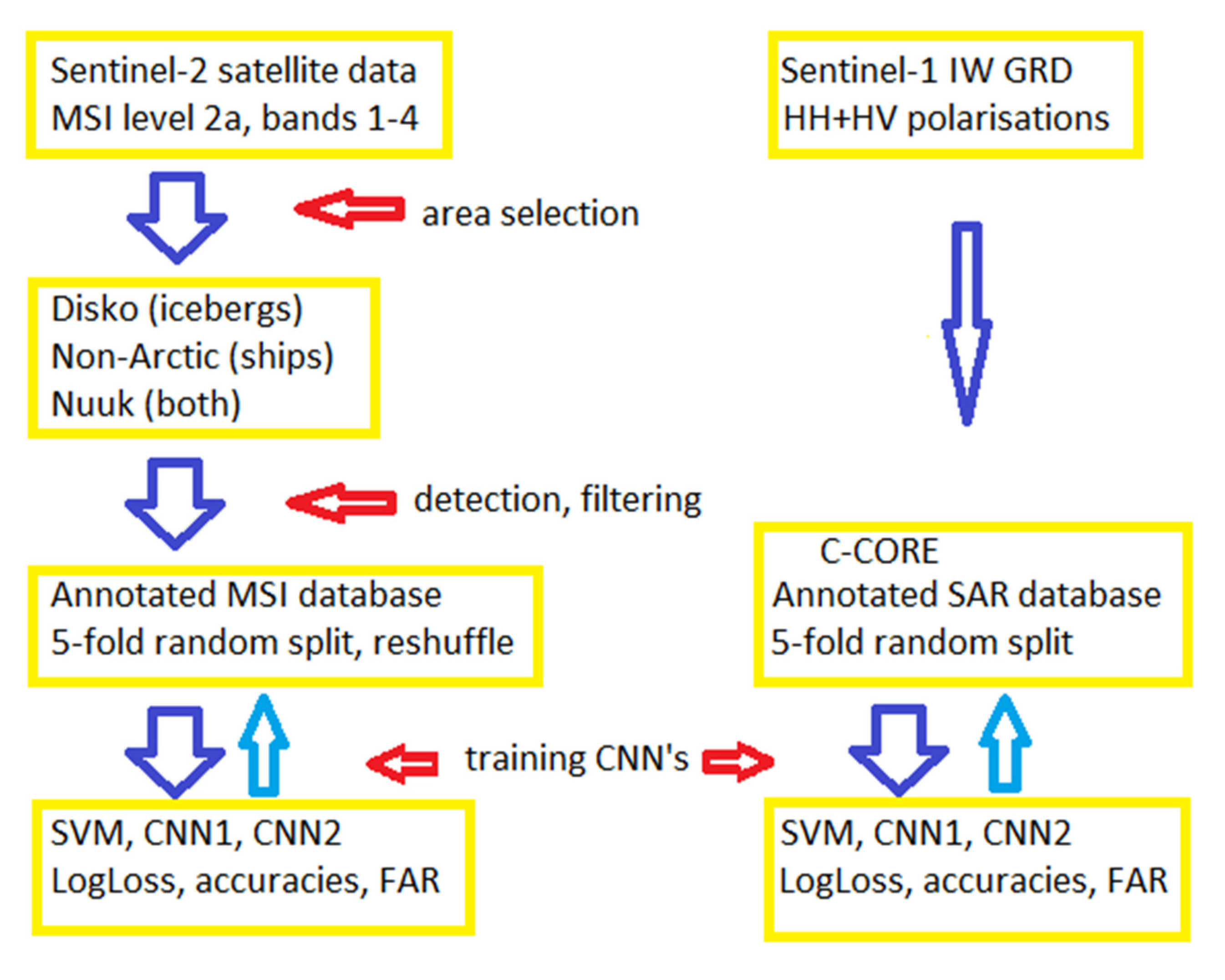
Figure 3 describes the flowchart in this work from data selection, ship and iceberg image detection for building an annotated dataset, the subsequent training of convolutional neural networks producing results for log-loss and accuracies. The methodology for building the database is described in Section 2.2, Section 2.3 and Section 2.4, whereas the methodology for finding and training the networks by optimization epoch by epoch as will be described in detail Section 3.
2.1. Sentinel-1 Synthetic Aperture Radar (SAR) Images
S1 carries the C-band SAR all-weather day-and-night imager [1]. As we are interested in small object classification and discrimination, we focus on analyzing the processed level-1 high-resolution ground range detected (GRDH) interferometric wide (IW) swath S1 images with 20 × 22 m resolution, and pixel spacing l = 10 m. These are mega- to giga-pixel images with 16-bit grey levels.
One cannot build a good SAR dataset as easily as in the MSI case described below, where we select images in the Arctic with icebergs only and images of ice-free oceans with ships only. This is because S1 data from Arctic regions are almost exclusively HH + HV polarized whereas they are VV+VH polarized in the rest of the world. This is deliberately chosen for better sea-ice detection and classification although it is unfortunate for ship-iceberg discrimination. Consequently, most icebergs are found in H and most ships in V polarizations. The different polarisation datatypes make the images different, and we find that it does not allow transfer learning and lead to erroneous classification [24]. For example, the background is different in H and V, and the neural networks may train itself to recognize the background instead of the objects. In that case, it would classify all ships in the Arctic as icebergs which we do not want.
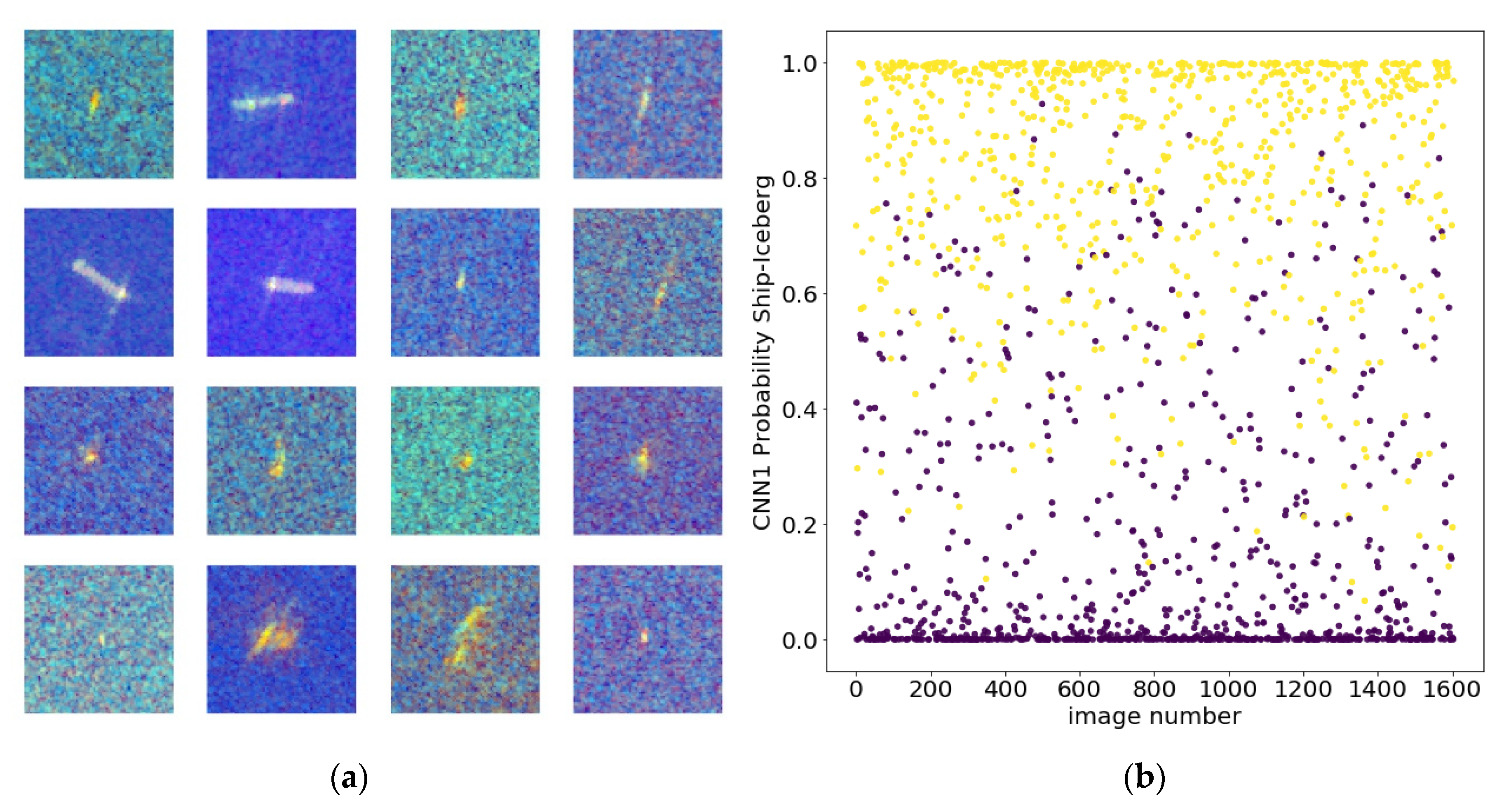
Fortunately, C-CORE have constructed an annotated and balanced dataset of S1 SAR images with 1604 ships and icebergs [2,20] (see Figure 4a). These were collected in S1 images along the east coast of Canada also referred to as the Iceberg Alley where titanic icebergs from Greenland endanger the ship traffic in the Atlantic ocean. This dataset has been extensively studied and discussed by more than 3000 groups participating in the Kaggle Statoil competition. We shall below describe results from deep learning analyses on this data.
The C-CORE satellite data consists of the two polarization images and the inclination angle by which the image was recorded. As the sea background backscatter generally decreases with the inclination angle it is useful information. However, the C-CORE inclination angles displayed a strange periodicity and grouping which could be exploited by algorithms designed to overfit this artifact in the constructed inclination data. As we consider this information unphysical, we exclude inclination angles in the following.
2.2. Sentinel-2 Multispectral Imager (MSI)
S2 carries the MSI [1] that records images in 13 multispectral bands with different resolutions. As we are interested in small object detection and tracking, we will focus on analyzing the high-resolution images, i.e., the 4 bands with 10 m pixel size. These are mega- to giga-pixel images with 16-bit grey levels. We analyze several S2 level 2A processed images from recent years covering Greenland, in particular the Disko Bay where there are thousands of icebergs and ice-floes but virtually no ships. In addition, we include non-Arctic seas around Denmark and the Faroe Islands where there are many ships but no icebergs. Finally, we include images around Nuuk, the Capital of Greenland, where there are both ships and icebergs present as will be discussed below. Before we merge these icebergs and ships in an annotated dataset, we filter out unwanted objects found by the detection algorithm.
Detection is performed in the combined red and near-infrared bands m = 3, 4, because they have high resolution and solar reflections from ships generally have high contrast in red a near-infrared with respect to the sea background. An object is defined spatially by the connected pixels with reflections above the background value plus a threshold T than can be related to a constant false alarm rate [18].
For each object, a small region of 75 × 75 pixels is extracted around the central object coordinate, such that it covers the object extent including wakes. The same region is now extracted for the 4 high-resolution bands m = 1, 2, 3, 4 (blue, green, red, and near-infrared) with spatial resolution 10 m. The other 6 bands with 20 m and the 3 bands with 60 m pixel resolution are not used in this analysis because they have less spatial information (see however [25]). For convenience, we combine the red and near-infrared bands m = 3, 4, to have the 3 color images as is commonly used for image recognition in neural nets. The two bands are close in wavelength and carry much of the same classification information as shown in [18]. By combining them in one layer, we include all the high-resolution MSI data. Including all the 13 bands in the input layers is a much more elaborate and time-consuming analysis that should be investigated in the future and compared to the present study.
A number of objects different from ships and icebergs may also be detected and have to be cleaned out by the detection by methods depending on the object:
- Land and sea-ice areas are removed by masking large areas with brightness above an adjusted threshold. Smearing is useful when backscatter/reflections are varying over land.
- Islands, wind turbines, and other stationary objects are removed by change detection, i.e., if they are detected at the same coordinates in another satellite image.
- Clouds in MSI images are minimized by choosing images with <10% cloud cover and setting a detection threshold sufficiently high.
- Coastal waves are removed by extending land smearing.
- Ocean waves are avoided by choosing weather conditions with low wind speed.
- Separated ship wakes are removed by only choosing the larges object in the image.
- If many objects appear in the 75 × 75 pixel window, it is most likely sea ice or clouds and they are removed.
- If several objects appear in the 75 × 75 pixel window, they are masked except for the central object. Hereby redundancy is avoided and objects are centered.
- Objects smaller than 4 pixels are removed whereby a large number of false alarms are removed. This sets a lower limit for ship and iceberg size detection. The sizes are, however, lower on average than those in the SAR images as shown in Figures 7a and 8a.
- Aircrafts are easily removed as they move fast and the temporal delay during acquisition separates the multispectral bands [25]. An aircraft appears twice separated in red and NIR both with high redness.
2.3. Semi-Supervised Data Augmentation
For testing in the Arctic, we include Sentinel-2 images around Nuuk, the capital of Greenland, where we detect and collect 350 ships and icebergs (see Figure 2 and Figure 5b). These are first classified by the list above in Section 2.2, and subsequently by manual classification methods described in Ref. [18]. Possible erroneous classifications are indicated by CNN and are visually inspected as will be discussed in Section 5.3. This part of the MSI dataset is semi-supervised. There are several smaller fishing boats en route from Nuuk out to fishing grounds with high speed and a distinct wake behind the boat. The ships and icebergs classified by this semi-supervised annotation are included in the MSI dataset where they play an important role as they provide small vessels in a real Arctic background of sea, icebergs, ice floes, rocks, and islands.
2.4. Data Augmentation by Rotation and Flipping
The 75 × 75 pixel square images can easily be rotated in steps of 90 degrees and flipped. Hereby the dataset is augmented by a factor of 4 × 2 = 8. Our classification algorithms do, however, calculate almost the same probabilities for the 8 augmented images, and therefore the resulting accuracy does not improve within the uncertainty of the epoch fluctuations discussed below. The main difference is a factor 8 increase in processing time. This lack of improvement indicates that the number of images is already sufficient and diverse in ship orientations that the rotational and mirror symmetry is implicit already in the non-augmented dataset.
In principle rotation and mirror symmetri is not generally valid when shadows are present in our satellite images and one should be careful with the proposed augmentations. The optical images are recorded from S2 in a sun-synchronous orbit flying almost north-south around noon in the local time zone. Thus shadows are almost northward in the Arctic and the only symmetry is left-right flipping. The SAR images are recorded from S1 right-looking between inclination angles 29–46° by active scanning almost east-west and so the only symmetry is up-down flipping. However, the ships and icebergs are not very tall and the angle of illumination sufficiently vertical. Therefore, their shadows short and only visible for large and tall objects in both the S1 nor the S2 data relative to their 10 m pixel resolution.
3. Methodology: Support Vector Machines (SVM) and Convolutional Neural Networks (CNN)
A comparison of SVM and CNN models [19] find that the ship classification accuracy generally improves with the number of features and parameters included in the model. In earlier publications [17,18] we have selected a few characteristic features that classify the objects well with the right parameter borders that were found by statistical methods very similar to Support Vector Machines (SVM). CNN automatically selects many more features that in principle is only limited by the millions of parameters in the model.
3.1. Support Vector Machines
Several spatial features are calculated for each object: the central position area A (the number of pixels with backscatter/reflectance above the threshold T mentioned in Section 2.2), orientation or heading angle, length L, and breadth B. Details of their calculation can be found in [17,18].
For the SAR data, the HH and HV radar backscatter from the object gives the total backscatter
and the cross-polarization ratio
The spectral features for the MSI data are the reflections in the four high-resolution bands m = B2, B3, B4, B8, corresponding to blue, green, red, and near-infrared bands, respectively. The total multispectral reflection from the object is
A useful feature for the object is the “redness” defined as the reflectance in the red and near-infrared with respect to the total reflectance
3.2. Convolutional Neural Networks (CNN)
More than 3000 deep neural networks participated in the Kaggle Statoil ship-iceberg classification competition [20] on the C-CORE SAR dataset. The best results were obtained by stacking several models and fine-tuning to the dataset. These models are very CPU time-consuming. Including inclination angles and overfitting their periodic behavior was also important.
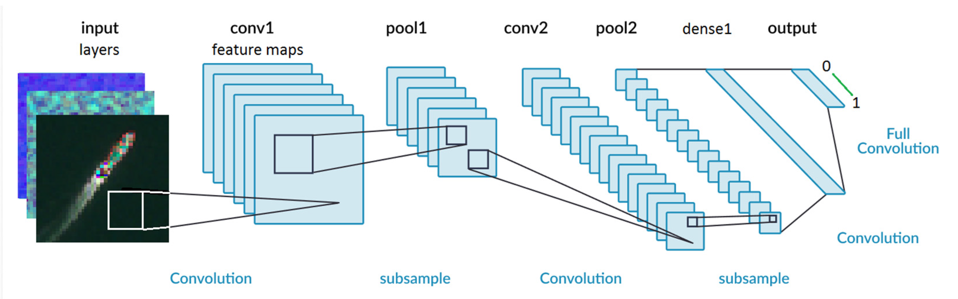
The purpose of this work is not to fine-tune deep neural nets but a more general study of various networks and the dependencies on the annotated datasets. Secondly, to find relatively simple and fast CNN with few parameters, yet robust towards new test data not included in training and validation. Finally, to compare CNN results for SAR and MSI datasets. We, therefore, restrict ourselves to single serial CNN, where we test a range of hyperparameters as layer types and depths, convolutional kernel sizes, pooling strides, activation, etc. (see Figure 6). The CNNs are trained from scratch because there are no previous analyses of MSI ship and iceberg data. From this survey, we have selected two of the best CNN’s referred to as CNN1 and CNN2. CNN1 has 562,241 parameters with layers and hyperparameters shown in Table 1. CNN2 has 1,134,081 parameters in 20 layers as shown in Table 2. The architectures are also similar to some of the best single serial CNN’s made available in the Kaggle contest [20,21,22,23] and with similar results for log-loss. We find that deeper networks with more parameters generally improve the accuracy at earlier epochs, but at the cost of longer computation time per epochs. For a fixed computation time the resulting accuracy is very similar for a wide range of deep neural networks within statistic fluctuations between epochs.
For a better comparison of classification for the SAR and MSI datasets, we will use the same CNN structure and hyperparameters, a number of images, pixel size, and number of training epochs. They will, however, be trained on the separate SAR and MSI datasets so that the CNN’s will learn different parameter sets.
We use 5-fold cross-validation for training and validation, i.e., 80% for training and 20% for validation chosen randomly in each epoch. As some of our data is grouped into icebergs and ships, we use random split and reshuffling. The Adam gradient descent optimizing algorithm with learning rate 0.0001, alpha1 = 0.9, alpha2 = 0.999, epsilon = 1 × 10⁻⁸, decay = 0) was used with batch size 24.
The binary cross-entropy or log-loss [26] was used as a cost function in the optimization algorithm.
The log-loss function has two classes which in our case are ship objects with and icebergs with , where i = 1,…, N; N is the number of objects. The log-loss is defined as the binary cross-entropy for the iceberg and ship classes [26]
here is the iceberg probability, which ranges between 0 for ships and 1 for icebergs, and is the ship probability.
Large scale computation analyses of hyperparameter dependences of a wide range of CNNs were performed using Keras Tensorflow on an Intel(R) Core(TM i5-8265U CPU with base frequency 1.60 GHz) and a GPU (GeForce GTX 1080) at DTU Compute. Specific CNN1 and CNN2 training could be performed on an ordinary PC. Up to 30 epochs were studied where after any improvement in validation accuracy was not observable within the epoch to epoch fluctuations. Some improvements in training accuracy could be observed due to the overfitting of training sets.
4. Classification Results
4.1. SVM
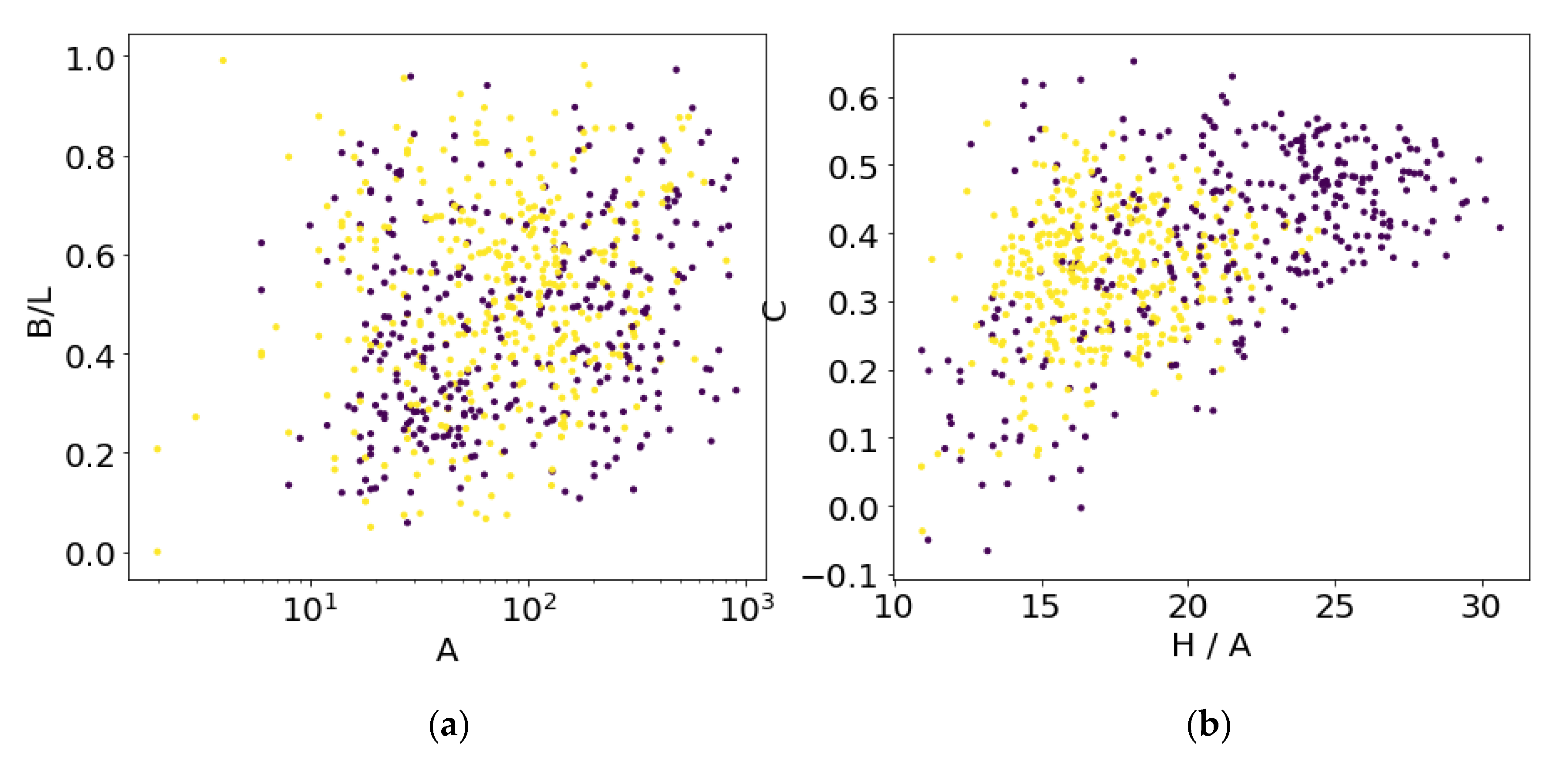
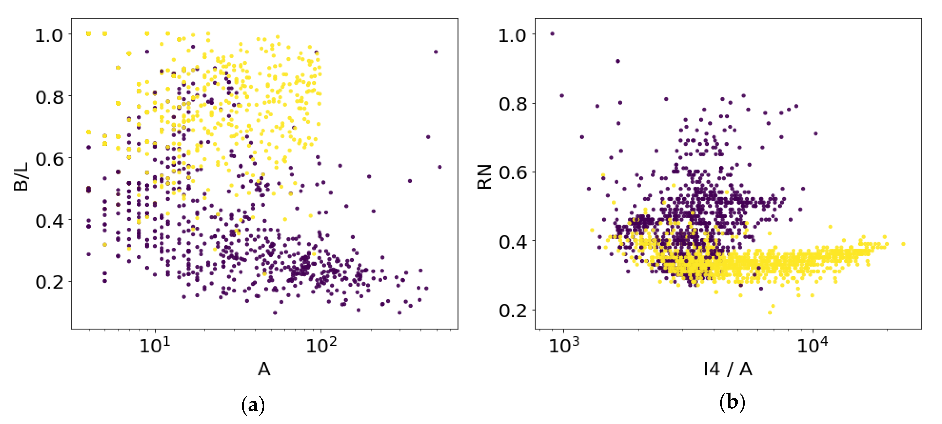
The optimal SVM hyperplane in the 4D feature parameter space cannot be plotted in the 2D plots of Figure 7 and Figure 8. The 4D parameter space consists of the 2D spatial parameters in Figure 7a and Figure 8a and 2D spectral parameters in Figure 7b and Figure 8b. As can be seen in Figure 7, the four SAR parameters do not separate ships from icebergs, and therefore the SVM accuracy is poor as given in Table 3. The separation is better for the MSI data in Figure 8, see Table 3. CNNs use many more spatial and spectral features than those shown in Figure 7 and Figure 8, which is why they are superior.
4.2. CNN
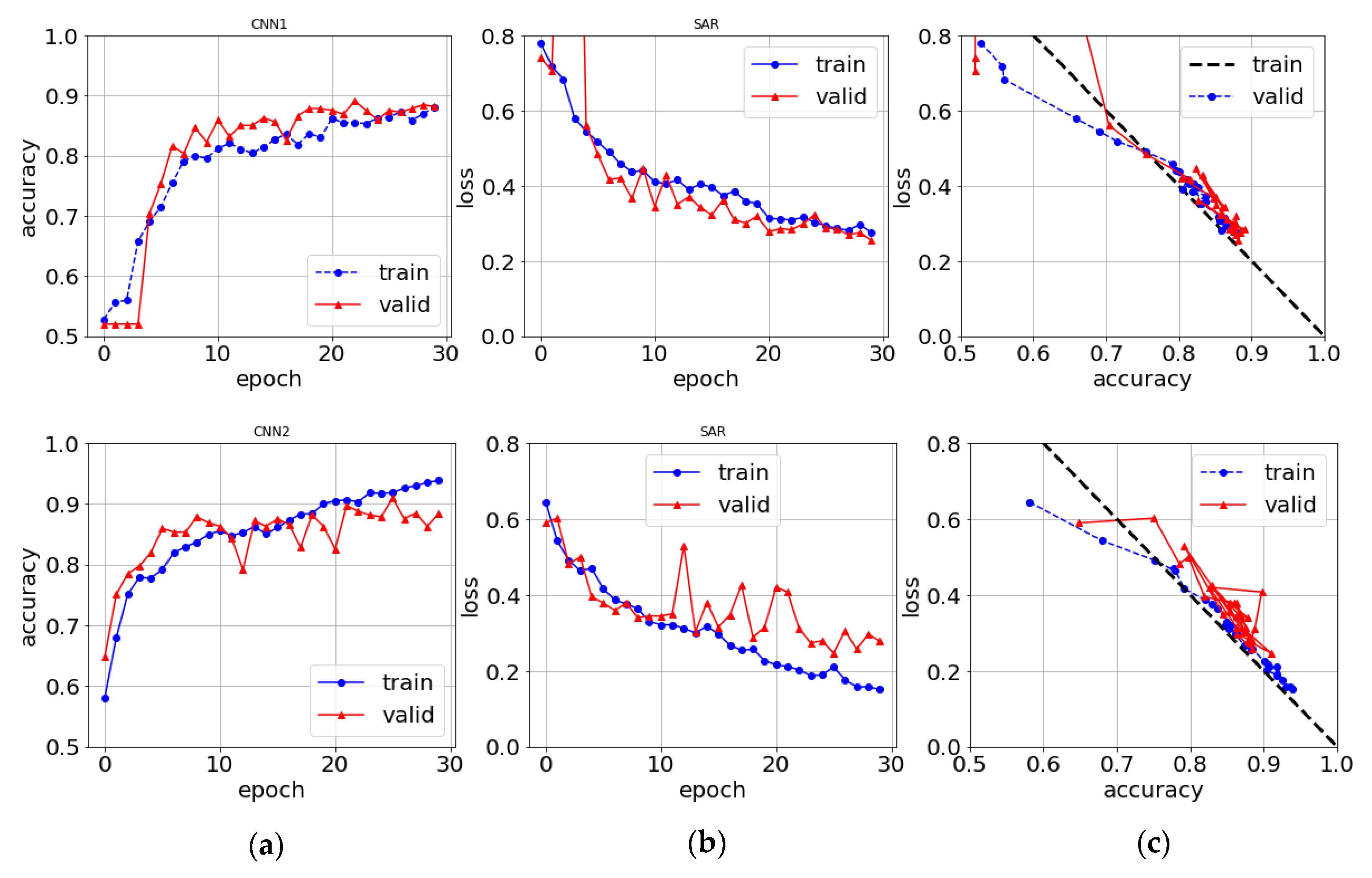
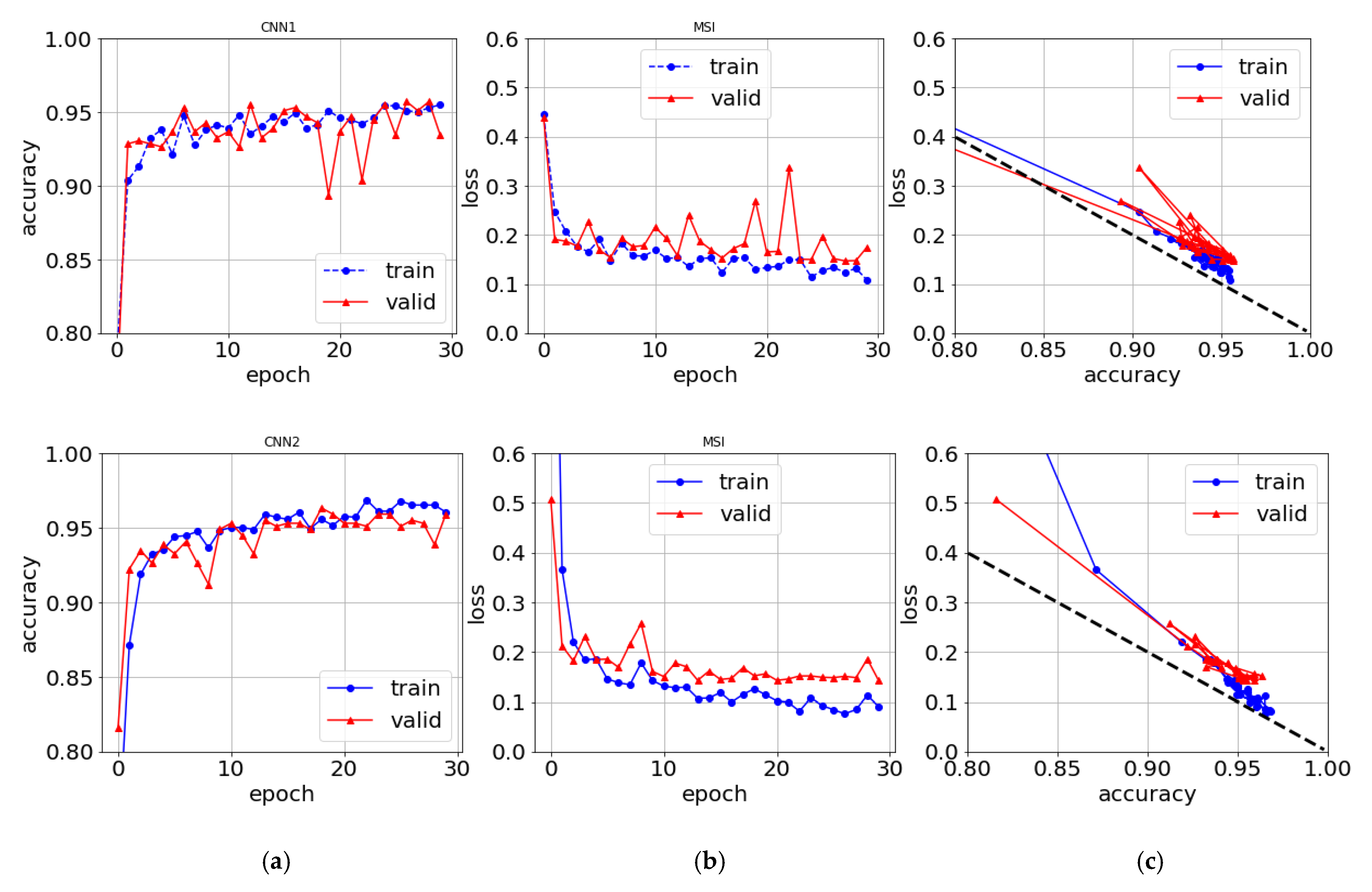
The training and validations result in Figure 9 and Figure 10 show quick convergence towards low log-loss. They also show the typically overfitting phenomena for neural networks, i.e., that training results are better validation for large epocs. Whereas the training results converge and continue to improve slowly with the number of epocs, the validation results stagnate at earlier epocs and fluctuate. This indicates that the models are overfitting. Both the overfitting and fluctuations are likely because the limited datasets are too small. The overfitting is worst for CNN2 as could be expected from the many more parameters, it has to fit. However, the three dropout layers reduce overfitting significantly.
The CNN2 trains better at earlier epocs as compared to CNN1. This is to be expected as CNN2 has more parameters and the epocs consume more CPU time. Relative to CPU time the two models train almost equally fast. The slightly better training results for CNN2 after 30 epocs can also be reached for CNN1 by increasing the number of epocs to an equivalent CPU time within statistical uncertainty and epoch-to-epoch fluctuations.
5. Discussion
The classification accuracies are summarized in Table 3 for SVM, CNN1, and CNN2 for both the SAR and MSI datasets. The datasets are balanced and we find that the models lead to approximately the same number of false negatives and false positives, i.e., the confusion matrices are almost symmetric. Consequently, the precision, recall, and F1 score differ little from the accuracy for both ships and icebergs, both datasets and all models.
5.1. SVM
Scatter plots of four selected features for the SAR dataset was shown in Figure 7. The area, breadth to length ratio, and the polarization ratio are not good classifiers, whereas the total backscatter per area is larger for ships than icebergs on average as found in earlier studies [2,3,17]. The 20 × 22 m resolution in the SAR data reduces the spatial resolution so that the elongated shape of ships is not a good discriminator. This confirms analyses in [17]. The resulting SVM classification accuracy is only 76% for the SAR dataset.
Scatter plots of the four selected features for the MSI dataset was shown in Figure 8. As described in [18] the object elongation and redness are good classifiers for discrimination ships and icebergs. The 10 m pixel resolution is observed for ships, which generally has a smaller breadth to length ratio than icebergs. However, when the object area is only a few pixels this classification breaks down. Ships also reflect more in the red and infrared bands than icebergs, however, again with some overlap for low reflective objects. Part of the reason is the mixing of sea and ship wakes in the object pixels. Running the support vector machine (SVM) classification on the four features, we obtain a classification accuracy of 82%.
The resulting SVM classification accuracies reflect the better resolution and more spectral bands in the MSI dataset, although one should be careful with a direct comparison. As can be seen from Figure 7 and Figure 8 the ships are on average larger in the SAR than in the MSI dataset. Selecting only larger ships in the MSI dataset would increase the accuracy considerably. Including more of the 13 multispectral bands with pan-sharpening [18] can improve the classification accuracy further.
5.2. CNN
CNNs include many more features than SVMs, and in principle up to as many as the number of parameters plus hyperparameters. Our results in Table 3 confirm that the classification generally improves with the number of features and parameters included when the chosen hyperparameters and training is done properly. Bentes et al. [19] analyzed TerraSAR data with 277 ships and 68 icebergs and found 88% score for an SVM with 16 features, 94% score for SVM with 60 features, and finally 97% score for CNN. Their CNN had only 5 layers but larger 128 × 128-pixel images, which was necessary for the TerraSAR images with 3 m ground resolution to cover the ships. Consider the higher resolution but fewer bands than MSI, their scores are compatible with our MSI accuracies.
More than 3000 deep neural networks participated in the Kaggle Statoil ship-iceberg classification competition [20]. The best models were stacked and fine-tuned to the dataset including inclination angles and were very CPU time-consuming. The best stacking models could press log-loss values down to 0.085 on the private leaderboard whereas the best single models reached 0.15 (0.135 for ResNet50) [20,21,22,23], which is close to our CNN2. Accuracies were only reported in a few cases and are compatible with our SAR results and Equation (5). The winners noted a flaw in the inclination angles, which they exploited to overfit the dataset. A large part of the inclination angles was periodic and grouped probably because they were artificially generated. For this reason, we did not include the inclination angles in the dataset resulting in a higher log-loss and lower accuracy. Future datasets should include real inclination angles as they contain useful information about ocean backscatter, which decreases with increasing inclination angle. Backscatter also increases with wind speed. The dataset should be extended to decrease fluctuations and overfitting.
The resulting minimal number of false alarms in CNN2 is about 4% for the MSI and 12% for the SAR datasets. The reason is as in the SVM case, that the MSI dataset has better resolution and more bands. This more than compensates the larger number of smaller objects in the MSI compared to SAR datasets, which are harder to classify.
5.3. Relations between Accuracy and Log-Loss in Neural Networks
When plotting the loss vs. accuracy as in Figure 9c and Figure 10c, we find that the training curves are very similar for both datasets and both CNN1 and CNN2 models. The curves lie almost on top of each other as do the validation curves until they saturate and fluctuate. Epoc-wise the CNN1 curve is translated to earlier epochs than the CNN2 curves, but not CPU time-wise as discussed above.
The universality of these curves can be understood as follows. We notice that the log-loss dependence on accuracy is fitted approximately by the simple relation
This simple relation between the classification accuracy and the log-loss measure in our neural networks reveals the relation between the underlying probability distributions, the optimization algorithm, the log-loss measure, and the resulting classification accuracies.
As we shall now show, this relation follows when the ship and iceberg probability distributions as shown in Figure 4b and Figure 5b have two components in every epoch:
- a classified component, where ships have probability 0 and icebergs probability 1.
- a non-classified component of ships and icebergs with probabilities evenly distributed between 0–1.
The log-loss function with two classes which in our case are ship objects with and icebergs with , were given in Equation (5) in terms of the iceberg probabilities , which range between 0 for ships and 1 for icebergs, and is the ship probability. Empirically the scatter plot distributions of in Figure 4b and Figure 5b are well described by two components. Let us model such a probability distribution for icebergs as
The two terms are the classified components in terms of a Kronecker delta function at p = 1, and the unclassified component given by a linear distribution with slope |α| < 1. Their weights are (1 − x) and x respectively so that P is normalized. The accuracy is the average of the probability
The log-loss value is by definition [26] the average of −log(p)
If we assume that the probability distribution for ships is symmetric by replacing p by (1 − p) in Equation (7), the result is identical for ships. Equation (9) is therefore also the combined ship and iceberg result as calculated by CNN. If the unclassified part is flat (zero slope α = 0), Equation (9) reduce to Equation (6).
The log-loss values of Equation (6) with slope 2 are plotted in Figure 9c and Figure 10c for every epoch. They fit the numerical results from the CNN models approximately with α = 0. If the non-classified part is not evenly distributed, for example, skewed towards correct classification, then the slope factor in Equation (9) decreases below 2. In the opposite case, the slope exceeds 2. The good agreement between the numerical log-loss values for every epoch and Equation (6) shown in Figure 9c and Figure 10c confirms the two-component probability distributions with a flat non-classified part for every epoch and not for just the final one. This is also confirmed by studying the probability distributions after every epoch. The slope is slightly larger than 2 for the MSI dataset in Figure 10c, which may be traced back to misclassifications in the Nuuk dataset as will be discussed in Section 5.4.
The training algorithm, therefore, acts as a “push-broom” (with some similarity to the push-broom recording technique used by the SAR and MSI sensors for sweeping sideways and collecting images in the swath along the satellite orbit around Earth) for every epoch in the sense, that it is sweeping some of the non-classified ships and icebergs to correct classification. Hereby, lowering the non-classified distribution evenly, reducing the log-loss and increasing the accuracy as given by Equation (6). A deeper CNN acts as a finer brush, where the final result is only limited by the quality or “roughness” of the dataset. The colorful and better resolved MSI dataset has better quality as is revealed by the finer CNN brushes.
5.4. Semi-Supervised Learning
The MSI satellite images over Nuuk, the capital of Greenland, contain both ships and icebergs that are not annotated. The SVM calculates the classification probabilities for all objects but we do not know a priori whether they truly are ships or icebergs. However, since the CNN classification is almost 100% accurate for the MSI dataset, we can to a very good approximation assume this annotation for the ships and icebergs. Using this annotation to calculate the accuracy in the SVM, gives 88% accuracy as shown in Table 3. It is better than for the annotated MSI dataset, which is expected as the semi-supervised annotation of the Nuuk dataset includes some of the SVM features.
Figure 5b shows that the CNN classification is best for the non-Arctic ship and Disko iceberg datasets whereas there are some misclassifications for the Nuuk dataset. A visual inspection shows that in several cases the CNN is correct but the semi-supervised annotation was erroneous. Correcting these annotations improves accuracy further. The erroneous annotations are also responsible for skewing the probability distribution and increasing the slope of Equation (9) above 2 as is observed in Figure 10c.
This shows the importance of a correctly annotated and large database of ships and icebergs, which further improve the accuracy and reduce the number of false alarms.
6. Summary and Outlook
The resulting accuracies for ship and iceberg classification give the false alarm rates which are crucial for Arctic surveillance, rescue services, etc. Reducing the number of false alarms relieves operational requirements and improves the real alarm effort. The assessment of the accuracies from SAR and MSI satellite data can also be used operationally in decision processes by choosing the targets with the highest probability or, for example, choosing to wait for a satellite pass with a more accurate MSI sensor if weather and time permits.
Deep neural nets are extremely effective for classifying ships and icebergs and superior to simpler statistical modes as SVM. CNN can be trained to high accuracy for a wide range of hyperparameters. Very deep networks can provide slightly better results but at the cost of increased CPU time and the risk of overfitting and increased sensitivity to the training and validation dataset.
Including small ships from Greenland is important as it greatly reduces the confusion with icebergs and false alarms. This indicates the importance of collecting an annotated database of ships and icebergs in situ for improving the classification, and include semi-supervised data with expert validation.
Augmentation by rotating and flipping images does not increase the accuracy noticeably for our datasets. Fluctuations and overfitting for large epocs do, however, indicate that the dataset is insufficient and should be extended to improve the accuracies further. Auxiliary data from inclination angles, sea state background, influence of weather conditions, the dependence of locality (e.g., tranquility in fjords), could also improve the classification.
A simple linear relation was found between the log-loss and accuracy values for both datasets, both CNN models and all epochs. The relation could be explained as a two-component probability distribution of ships and icebergs, where a constant unclassified part was gradually swept to correct classification in every epoch. It reveals the underlying relations between probabilities, the optimization algorithm, the log-loss measure, and resulting classification accuracies as well as possible erroneous annotations.
SAR imagery has the advantage that it sees through clouds day and night, whereas optical imagery generally has better resolution and more spectral bands. As a result, the classifications were significantly better for S2 MSI images than S1 SAR images. The operational requirement may favor one from the other, but a combination of both monitored over time can provide further intel for search, detection, and recognition. For example, if a ship has been detected and correlated with AIS data at an earlier time, we can use its MSI and/or SAR features as a “fingerprint” for subsequent searches in satellite imagery in case it turns into dark ship mode. Over time there is a better chance to find S2 images with low cloud coverage, where the ship can be better identified for later use. Further study and comparison of detection, classification, spatial and temporal coverage are thus important for optimizing the intelligence, surveillance, and reconnaissance operations.
Funding
This research received external funding from the co-finance research program under the Danish Defense Acquisition & Logistics Org.
Acknowledgments
To ESA Copernicus for use of Sentinel-1 and -2 data covering oceans between Greenland and Denmark, and to the Arctic Command Denmark for support and interest.
Conflicts of Interest
The author declares no conflict of interest. We fulfill the condition in the Sentinel Data Legal Notice [1].
References
- ESA Copernicus Program, Sentinel Scientific Data Hub. Available online: https://schihub.copernicus.eu (accessed on 1 July 2020).
- C-CORE. Summary of Previous Research in Iceberg and Ship Detection and Discrimination in SAR. DRDC Report No: R-13-060-1098. 2013. Available online: https://cradpdf.drdc-rddc.gc.ca/PDFS/unc196/p800002_A1b.pdf (accessed on 1 July 2020).
- Hannevik, T.N.A. Literature Review on Ship and Ice Discrimination. FFI Report 17/16310. 2017. Available online: https://ffi-publikasjoner.archive.knowledgearc.net/handle/20.500.12242/2321 (accessed on 1 July 2020).
- Brekke, C.; Weydahl, D.J.; Helleren, Ø.; Olsen, R. Ship traffic monitoring using multipolarisation satellite SAR images combined with AIS reports. In Proceedings of the 7th European Conference on Synthetic Aperture Radar (EUSAR), Friedrichshafen, Germany, 2–5 June 2008. [Google Scholar]
- Santamaria, C.; Greidanus, H.; Fournier, M.; Eriksen, T.; Vespe, M.; Alvarez, M.; Arguedas, V.F.; Delaney, C.; Argentieri, P. Sentinel-1 Contribution to Monitoring Maritime Activity in the Arctic. In Proceedings of the ESA Living Planet Symposium; ESA SP-740, Prague, Czech Republic, 9–13 May 2016. [Google Scholar]
- Park, K.; Park, J.; Jang, J.; Lee, H.; Oh, S.; Lee, M. Multi-Spectral Ship Detection Using Optical, Hyperspectral, and Microwave SAR Remote Sensing Data in Coastal Regions. Sustainability 2018, 10, 4064. [Google Scholar] [CrossRef] [Green Version]
- Brusch, S.; Lehner, S.; Fritz, T.; Soccorsi, M.; Soloviev, A.; Schie, B. Ship surveillance with TerraSAR-X. IEEE Trans. Geosci. Remote Sens. 2010, 49, 1092–1103. [Google Scholar] [CrossRef]
- Saur, G.; Teutsch, M. SAR signature analysis for TerraSAR-X-based ship monitoring. In Image and Signal Processing for Remote Sensing XVI; 78301O-1; SPIE—International Society for Optics and Photonics: Bellingham, WA, USA, 2010; Volume 7830. [Google Scholar]
- Chang, Y.-L.; Anagaw, A.; Chang, L.; Wang, Y.C.; Hsiao, C.-Y.; Lee, W.-H. Ship Detection Based on YOLOv2 for SAR Imagery. Remote Sens. 2019, 11, 786. [Google Scholar] [CrossRef] [Green Version]
- Ma, M.; Chen, J.; Liu, W.; Yang, W. Ship Classification and Detection Based on CNN Using GF-3 SAR Images. Remote Sens. 2018, 10, 2043. [Google Scholar] [CrossRef] [Green Version]
- Dai, W.; Mao, Y.; Yuan, R.; Pu, X.; Li, C.; Dai, W.; Mao, Y.; Yuan, R.; Liu, Y.; Pu, X.; et al. A Novel Detector Based on Convolution Neural Networks for Multiscale SAR Ship Detection in Complex Background. Sensors 2020, 2, 2547. [Google Scholar] [CrossRef] [PubMed]
- Lin, Z.; Ji, K.; Leng, X.; Kuang, G. Squeeze and Excitation Rank Faster R-CNN for Ship Detection in SAR Images. IEEE Geosci. Remote Sens. Lett. 2019, 16, 751–755. [Google Scholar] [CrossRef]
- Xie, X.; Li, B.; Wei, X. Ship Detection in Multispectral Satellite Images under Complex Environment. Remote Sens. 2020, 12, 792. [Google Scholar] [CrossRef] [Green Version]
- Yang, X.; Su, H.; Fu, K.; Yang, J.; Sun, X.; Yan, M.; Guo, Z. Automatic Ship Detection in Remote Sensing Images from Gogle Earth of Complex Scenes Based on Multiscale Rotation Dense Feature Pyramid Networrks. Remote Sens. 2018, 10, 132. [Google Scholar] [CrossRef] [Green Version]
- Zhu, C.; Zhou, H.; Wang, R.; Guo, J. A novel hierarchical method of ship detection from spaceborne optical image based on shape and texture features. IEEE Trans. Geosci. Remote Sens. 2010, 48, 3446–3456. [Google Scholar] [CrossRef]
- Denbina, M.; Collins, M.J.; Atteia, G. On the Detection and Discrimination of Ships and Icebergs Using Simulated Dual-Polarized RADARSAT Constellation Data. Can. J. Remote Sens. 2015, 41, 5. [Google Scholar] [CrossRef]
- Heiselberg, H. Ship-Iceberg Detection & Classification in Sentinel-1 SAR Images. In Proceedings of the 13th International Conference on Marine Navigation and Safety of Sea Transportation, Gdynia, Poland, 12–14 June 2019; Volume 14, p. 235. [Google Scholar]
- Heiselberg, P.; Heiselberg, H. Ship-Iceberg discrimination in Sentinel-2 multispectral imagery. Remote Sens. 2017, 9, 1156. [Google Scholar] [CrossRef] [Green Version]
- Bentes, C.; Frost, A.; Velotto, D.; Tings, B. Ship-Iceberg discrimination with convolutional neural networks in high resolution SAR images. In Proceedings of the EUSAR 2016: 11th European Conference on Synthetic Aperture Radar, Hamburg, Germany, 6–9 June 2016. [Google Scholar]
- Ship-Iceberg Classifier Challenge in Machine Learning. 2018. Available online: https://www.kaggle.com/c/statoil-iceberg-classifier-challenge (accessed on 1 July 2020).
- Yang, X.; Ding, J. A Computational Framework for Iceberg and Ship Discrimination: A Case Study on Kaggle Competition. IEEE Access 2020, 8, 82320. [Google Scholar] [CrossRef]
- Kang, M.; Ji, K.; Leng, X.; Lin, A. Contextual Region-based Convolutional Neural Network with Multilayer Fusion for SAR Ship Detection. Remote Sens. 2017, 9, 860. [Google Scholar] [CrossRef] [Green Version]
- Jang, H.; Kim, S.; Lam, T. Kaggle Competitions: Author Identification and Statoil/C-CORE Iceberg Classifier Challenge, School of Informatics, Computing, and Engineering; Datamining B565 Fall; Indiana University: Bloomington, IN, USA, 2017. [Google Scholar]
- Mogensen, N. Ship-Iceberg Discrimination in Sentinel-1 SAR Imagery Using Convolutional Neural Networks and Transfer Learning. Master’s Thesis, Technical University of Denmark, Kongens Lyngby, Denmark, 2019. [Google Scholar]
- Heiselberg, H. Aircraft and Ship Velocity Determination in Sentinel-2 Multispectral Images. Sensors 2019, 19, 2873. [Google Scholar] [CrossRef] [Green Version]
- A Definition of Binary Log-Loss. Available online: https://www.kaggle.com/wiki/LogLoss (accessed on 1 July 2020).
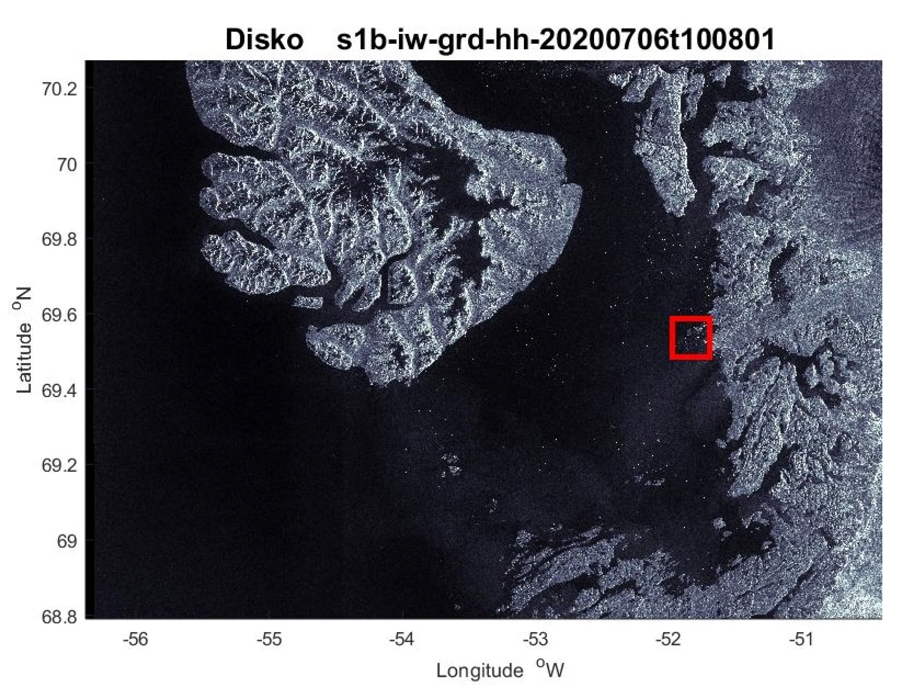
Figure 1.
Sentinel-1 (S1) high-resolution ground range detected (GRDH) interferometric wide (IW) synthetic-aperture radar (SAR) tile of the Disko Bay. The red box indicates the Ilulissat Icefjord, probably the fastest-flowing ice glacier and iceberg producer in the world.
Figure 1.
Sentinel-1 (S1) high-resolution ground range detected (GRDH) interferometric wide (IW) synthetic-aperture radar (SAR) tile of the Disko Bay. The red box indicates the Ilulissat Icefjord, probably the fastest-flowing ice glacier and iceberg producer in the world.

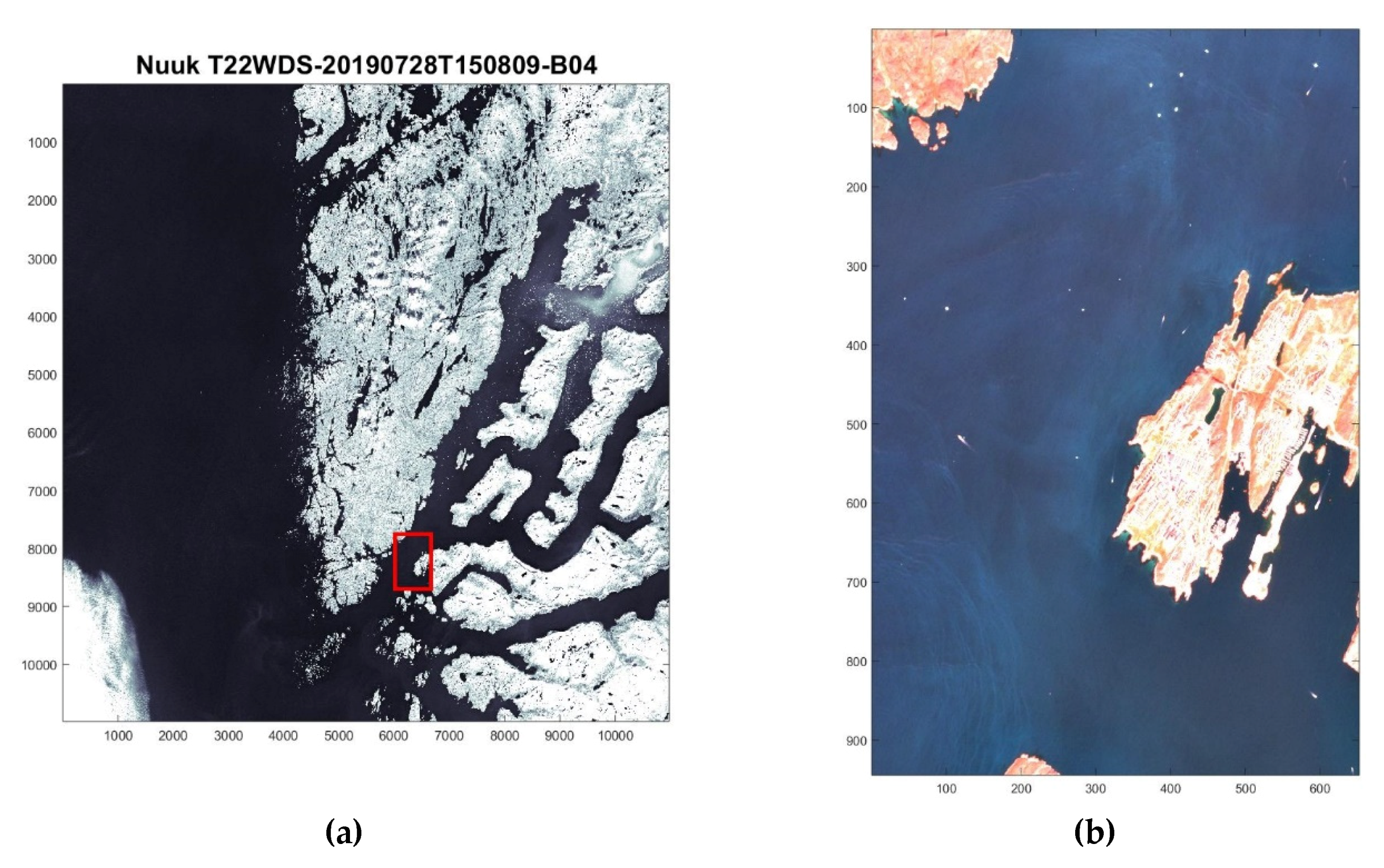
Figure 2.
(a) ESA Copernicus SciHub Sentinel-2 tile image around Nuuk, the capital of Greenland. The red box shows the inset on the right (b), and the RGB image shows icebergs and ships with wakes around Nuuk.
Figure 2.
(a) ESA Copernicus SciHub Sentinel-2 tile image around Nuuk, the capital of Greenland. The red box shows the inset on the right (b), and the RGB image shows icebergs and ships with wakes around Nuuk.

Figure 3.
Flowchart: data selection, ship and iceberg image detection for building an annotated dataset, the subsequent training of convolutional neural networks producing results for log-loss and accuracies.
Figure 3.
Flowchart: data selection, ship and iceberg image detection for building an annotated dataset, the subsequent training of convolutional neural networks producing results for log-loss and accuracies.

Figure 4.
(a) Samples of ships and icebergs(top and bottom rows respectively) false-color images from the SAR dataset; (b) Scatter plots of the annotated S1 SAR dataset of ships (blue) and icebergs (yellow). The probabilities range from 0 (ship) to 1 (iceberg) and are calculated by the deep neural network described below and plotted vs. image number.

Figure 5.
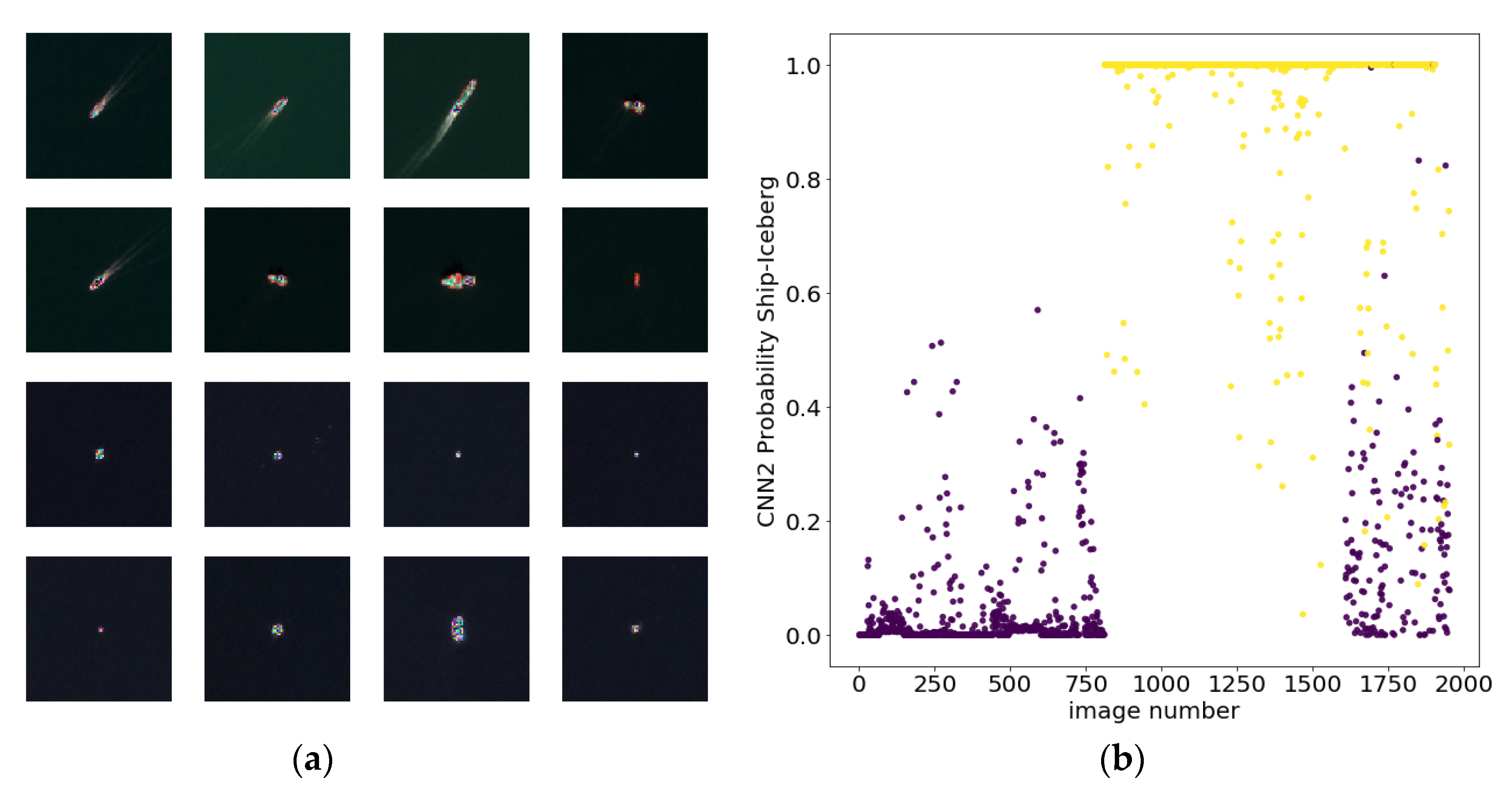
As Figure 4 but for the Sentinel-2 multispectral imaging (MSI) dataset. (a) RGB images of ships and icebergs. The scatter plot in (b) shows the ship, iceberg, and Nuuk datasets merged sequentially by image number.
Figure 5.
As Figure 4 but for the Sentinel-2 multispectral imaging (MSI) dataset. (a) RGB images of ships and icebergs. The scatter plot in (b) shows the ship, iceberg, and Nuuk datasets merged sequentially by image number.

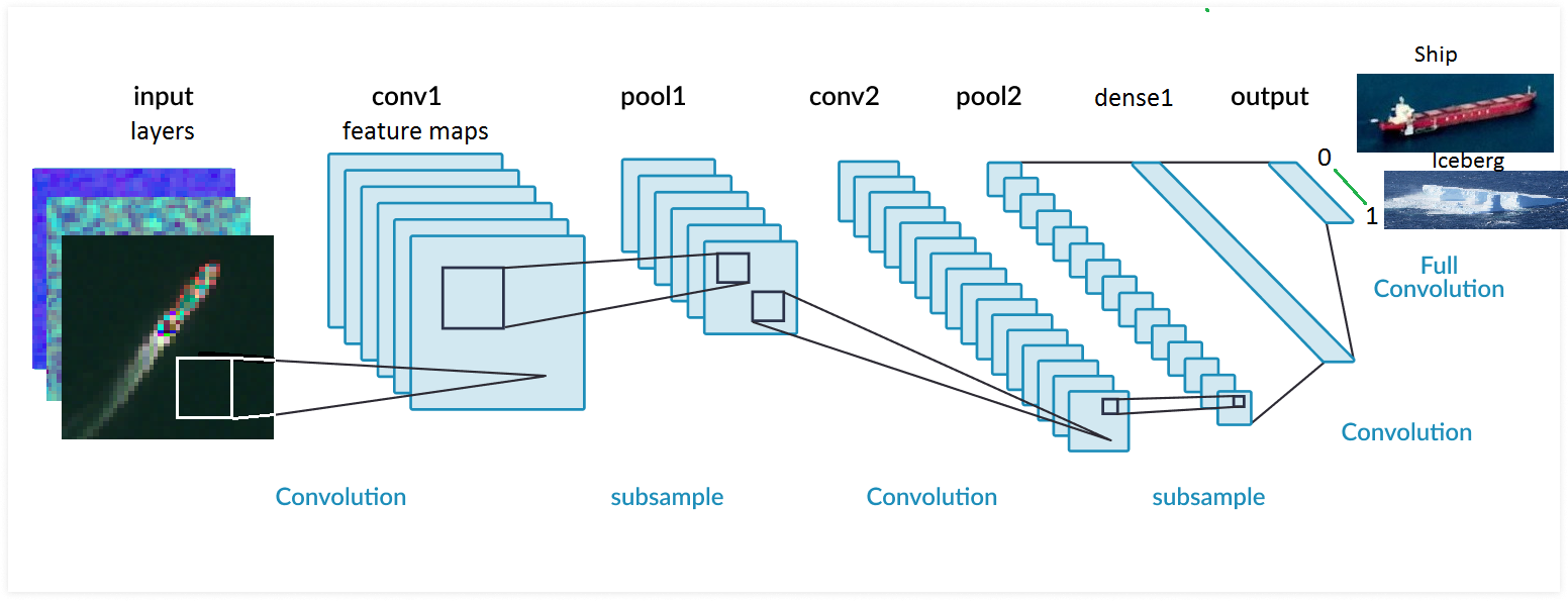
Figure 6.
Sketch of a simple convolutional neural network with 3 input layers (RGB), two 2D convolutional layers followed by two pooling layers, one final dense layer. The output is a probability ranging from 0 (ship) to 1 (iceberg).
Figure 6.
Sketch of a simple convolutional neural network with 3 input layers (RGB), two 2D convolutional layers followed by two pooling layers, one final dense layer. The output is a probability ranging from 0 (ship) to 1 (iceberg).

Figure 7.
Scatter plots of SAR ships (blue) and icebergs (yellow) classified according to (a) breadth B to length L ratio vs. area A, (b) cross-polarization HV/H vs. average object backscatter H/A (in dB).
Figure 7.
Scatter plots of SAR ships (blue) and icebergs (yellow) classified according to (a) breadth B to length L ratio vs. area A, (b) cross-polarization HV/H vs. average object backscatter H/A (in dB).

Figure 8.
Scatter plot of MSI ships (blue) and icebergs (yellow) classified according to (a) breadth to length ratio vs. area; (b) redness vs. average object reflection.
Figure 8.
Scatter plot of MSI ships (blue) and icebergs (yellow) classified according to (a) breadth to length ratio vs. area; (b) redness vs. average object reflection.

Figure 9.
CNN1 top and CNN2 bottom row for the SAR dataset. (a) Accuracy and (b) Log-loss vs. epochs. (c) Log-loss vs. accuracy. The dashed curve is Equation. (6)—see text.
Figure 9.
CNN1 top and CNN2 bottom row for the SAR dataset. (a) Accuracy and (b) Log-loss vs. epochs. (c) Log-loss vs. accuracy. The dashed curve is Equation. (6)—see text.

Figure 10.
As Figure 9 but for the MSI dataset.
Figure 10.
As Figure 9 but for the MSI dataset.


Table 1.
CNN1 layers and hyperparameters. Input channels are HH + HV for SAR and RGB for MSI datasets, where R includes both the red and near-infrared high-resolution bands.
Table 1.
CNN1 layers and hyperparameters. Input channels are HH + HV for SAR and RGB for MSI datasets, where R includes both the red and near-infrared high-resolution bands.
| Layer | Image Size | Channels | Kernel or Pool Size | Strides | Activation | Parameters |
|---|---|---|---|---|---|---|
| Input | 75 × 75 | 2 or 3 | ||||
| Conv2D | 73 × 73 | 64 | 3 × 3 | ReLu | 1792 | |
| MaxPool2D | 36 × 36 | 64 | 3 × 3 | (2,2) | 0 | |
| Dropout 0.2 | 36 × 36 | |||||
| Conv2D | 34 × 34 | 128 | 3 × 3 | ReLu | 73,856 | |
| MaxPool2D | 17 × 17 | 128 | 2 × 2 | (2,2) | 0 | |
| Dropout 0.1 | 0 | |||||
| Conv2D | 15 × 15 | 128 | 3 × 3 | ReLu | 147,584 | |
| MaxPool2D | 7 × 7 | 128 | 2 × 2 | (2,2) | 0 | |
| Dropout 0.1 | ||||||
| Conv2D | 5 × 5 | 64 | 3 × 3 | ReLu | 73,792 | |
| MaxPool2D | 2 × 2 | 64 | 2 × 2 | (2,2) | 0 | |
| Dropout 0.2 | ||||||
| Flatten | 1 × 1 | 256 | 0 | |||
| Dense | 512 | ReLu | 131,584 | |||
| Batch renormalization | 512 | 2048 | ||||
| Dropout 0.2 | ||||||
| Dense | 256 | ReLu | 131,328 | |||
| Dropout 0.2 | 0 | |||||
| Dense | 1 | Sigmoid | 257 | |||
| 561,217 |
Table 2.
As Table 1 but for layers and hyperparameters of CNN2.
Table 2.
As Table 1 but for layers and hyperparameters of CNN2.
| Layer | Image Size | Channels | Kernel or Pool Size | Strides | Activation | Parameters |
|---|---|---|---|---|---|---|
| Input | 75 × 75 | 2 or 3 | ||||
| Conv2D | 73 × 73 | 64 | 3 × 3 | ReLu | 1792 | |
| Conv2D | 71 × 71 | 64 | 3 × 3 | ReLu | 36,928 | |
| Conv2D | 69 × 69 | 64 | 3 × 3 | ReLu | 36,928 | |
| MaxPool2D | 34 × 34 | 64 | 3 × 3 | (2,2) | 0 | |
| Conv2D | 32 × 32 | 128 | 3 × 3 | ReLu | 73,856 | |
| Conv2D | 30 × 30 | 128 | 3 × 3 | ReLu | 147,584 | |
| Conv2D | 28 × 28 | 128 | 3 × 3 | ReLu | 147,584 | |
| MaxPool2D | 14 × 14 | 128 | 2 × 2 | (2,2) | 0 | |
| Dropout 0.1 | 0 | |||||
| Conv2D | 12 × 12 | 128 | 3 × 3 | ReLu | 147,584 | |
| MaxPool2D | 6 × 6 | 128 | 2 × 2 | (2,2) | 0 | |
| Conv2D | 4 × 4 | 128 | 3 × 3 | ReLu | 147,584 | |
| MaxPool2D | 2 × 2 | 128 | 2 × 2 | (2,2) | 0 | |
| Dropout 0.2 | ||||||
| Flatten | 1 × 1 | 512 | 0 | |||
| Dense | 512 | ReLu | 262,656 | |||
| Dense | 256 | ReLu | 131,328 | |||
| Dropout 0.2 | 0 | |||||
| Dense | 1 | Sigmoid | 257 | |||
| 1,134,081 |
Table 3.
Accuracies in % for the models and datasets. For the Nuuk MSI dataset, the SVM accuracy is calculated by assuming that CNN is 100% accurate (see text).
Table 3.
Accuracies in % for the models and datasets. For the Nuuk MSI dataset, the SVM accuracy is calculated by assuming that CNN is 100% accurate (see text).
| Accuracy | SVM | CNN1 Train/Valid | CNN2 Train/Valid |
|---|---|---|---|
| S1 SAR | 76% | 87/86% | 94/88% |
| S2 MSI | 82% | 96/95% | 97/96% |
| Nuuk | 88% | (100%) | (100%) |
© 2020 by the author. Licensee MDPI, Basel, Switzerland. This article is an open access article distributed under the terms and conditions of the Creative Commons Attribution (CC BY) license (http://creativecommons.org/licenses/by/4.0/).
Share and Cite
MDPI and ACS Style
Heiselberg, H. Ship-Iceberg Classification in SAR and Multispectral Satellite Images with Neural Networks. Remote Sens. 2020, 12, 2353. https://0-doi-org.brum.beds.ac.uk/10.3390/rs12152353
AMA Style
Heiselberg H. Ship-Iceberg Classification in SAR and Multispectral Satellite Images with Neural Networks. Remote Sensing. 2020; 12(15):2353. https://0-doi-org.brum.beds.ac.uk/10.3390/rs12152353
Chicago/Turabian StyleHeiselberg, Henning. 2020. "Ship-Iceberg Classification in SAR and Multispectral Satellite Images with Neural Networks" Remote Sensing 12, no. 15: 2353. https://0-doi-org.brum.beds.ac.uk/10.3390/rs12152353
Note that from the first issue of 2016, this journal uses article numbers instead of page numbers. See further details here.