A Novel Classification Extension-Based Cloud Detection Method for Medium-Resolution Optical Images

Abstract

Accurate cloud detection using medium-resolution multispectral satellite imagery (such as Landsat and Sentinel data) is always difficult due to the complex land surfaces, diverse cloud types, and limited number of available spectral bands, especially in the case of images without thermal bands. In this paper, a novel classification extension-based cloud detection (CECD) method was proposed for masking clouds in the medium-resolution images. The new method does not rely on thermal bands and can be used for masking clouds in different types of medium-resolution satellite imagery. First, with the support of low-resolution satellite imagery with short revisit periods, cloud and non-cloud pixels were identified in the resampled low-resolution version of the medium-resolution cloudy image. Then, based on the identified cloud and non-cloud pixels and the resampled cloudy image, training samples were automatically collected to develop a random forest (RF) classifier. Finally, the developed RF classifier was extended to the corresponding medium-resolution cloudy image to generate an accurate cloud mask. The CECD method was applied to Landsat-8 and Sentinel-2 imagery to test the performance for different satellite images, and the well-known function of mask (FMASK) method was employed for comparison with our method. The results indicate that CECD is more accurate at detecting clouds in Landsat-8 and Sentinel-2 imagery, giving an average F-measure value of 97.65% and 97.11% for Landsat-8 and Sentinel-2 imagery, respectively, as against corresponding results of 90.80% and 88.47% for FMASK. It is concluded, therefore, that the proposed CECD algorithm is an effective cloud-classification algorithm that can be applied to the medium-resolution optical satellite imagery.

1. Introduction

Optical remote sensing data ranging from the visible to shortwave infrared are widely used for surface cover mapping, surface parameters estimation, and ecosystem monitoring [1,2,3,4]. Nowadays, with the increasing number of medium-resolution optical sensors, the opportunity for finer monitoring of the global environmental has been provided [5,6,7,8]. Nevertheless, the images from these sensors are usually contaminated by clouds. The existence of this contamination obscures the ground-surface reflectance and reduces the accuracy of the use of optical images in various applications [9,10]. Therefore, accurately identifying and masking clouds is a preprocessing step that should be carried out before using optical imagery.

In general, clouds appear as bright pixels in optical imagery. They have a higher spectral reflectance and lower brightness temperature (BT) than other surface cover types [11,12,13,14]. However, due to the heterogeneity of images and the variable transparency of clouds, the confusion caused by non-cloud bright surfaces and thin clouds, which are difficult to detect, makes it difficult to automatically identify cloud pixels [1,15,16,17,18]. Although the use of thermal infrared bands can improve the accuracy of cloud detection, this generally only works well for thick, cold clouds and the commission error in high mountain regions may be high [14,15]. In addition, for those optical sensors that do not have thermal infrared bands (such as Sentinel-2, SPOT4-HRVIR), effectively mitigating the disturbances caused by bright non-cloud surfaces remains a challenge [1,15].

Nowadays, many cloud-detection methods have been developed for the accurate flagging of clouds. These methods can be roughly divided into two categories: rule-based algorithms [1,9,11,13,14,15,19,20,21] and machine learning-based algorithms [22,23,24,25,26,27,28].

Most existing cloud-detection methods that belong to the first category are mono-temporal methods [15]. For example, Zhu et al. [12] proposed the function of mask (FMASK) algorithm to detect clouds in Landsat and Sentinel-2 imagery. Irish et al. [20] developed an automatic cloud cover assessment (ACCA) algorithm for classifying clouds in Landsat-7 imagery. These approaches are simple to implement, but they often suffer from non-cloud bright surface commission and thin cloud omission [12,29]. To reduce the confusion caused by non-cloud surfaces, several multi-temporal methods were also proposed [1,30,31], such as multi-temporal mask (Tmask) [10] and multi-temporal cloud detection (MTCD) [21]. These multi-temporal methods require either a cloud-free image or multiple cloud-free observations [21,31]. However, for satellites with long revisit periods (such as Landsat, GaoFen, SPOT), this requirement is difficult to meet. In addition, it is difficult to automatically know whether or not cloud-free observations are available before using one of these methods [1].

To produce more accurate cloud masks, machine learning techniques for cloud detection are introduced [22,23] For instance, Joshi et al. [22] used the support vector machine (SVM) method to mask clouds in Landsat-8. Ghasemian et al. [32] proposed a random forest-based cloud detection method to flag clouds in Landsat and MODIS. Recently, as a subset of machine learning, some complex deep learning algorithms have also been used for cloud detection—for example, Li et al. [23] employed a deep learning-based method to detect clouds for different medium and high resolution remote sensing images. These machine-learning methods require sufficient labeled samples to determine the parameters of classification models [24]. When the training dataset is sufficiently large and representative, machine learning-based algorithms outperform the rule-based ones, even without using the thermal infrared bands [22,24]. However, due to the difficulties in separating cloud pixels from non-cloud pixels, it is hard to automatically select accurate cloud and non-cloud training samples for each scene [24,33]. Therefore, machine learning-based methods are not as popular as the rule-based ones.

Taking into account the above, it can be said that the machine learning-based approaches can achieve a higher accuracy than the rule-based ones, but the lack of accurate and representative training datasets is a major drawback hindering the development of machine-learning based methods.

To address the drawbacks mentioned above of machine-learning methods, some researchers have employed a spectral signature extension strategy to compensate for the problem of insufficient training samples [23,24]. They collect training samples from existing training datasets, and extend the spectral signatures of the samples to classify clouds in other scenes from different spatial and temporal domains. This strategy can produce great savings in the time and labor costs involved in building an extensive training set; however, it is not suitable for scenes that are spatially or temporally different from the training datasets [23,34,35]. Recently, Zhang et al. [36] proposed a novel classification extension strategy to overcome the difficulty of collecting training samples for large-scale land cover mapping. They developed classification models from low-resolution ls, and extended the classification models to the corresponding medium-resolution images for land cover mapping. Since they used low-resolution satellite imagery (with short revisit period) to develop a local adaptive classifier for each medium-resolution image, their strategy is able to overcome the spatial and temporal limitations of the signature extension strategy [36,37]. Because cloud pixels can be effectively extracted with the support of prior surface reflectance [17,21,31], and the low-resolution images provide prior spectral signatures of surfaces at any period [17,36,38], it is possible to develop a cloud classification model at a low-resolution level for each medium-resolution image.

Inspired by the previous studies, in this work we advanced the classification extension strategy from land cover mapping to the field of cloud detection, and proposed a novel classification extension-based cloud detection (CECD) method for medium-resolution imagery. To achieve this goal, training samples were first automatically extracted from low-resolution images. Then, based on the training samples and the reflectance spectra in the resampled cloudy imagery, local adaptive random forest (RF) classifiers were trained at a low-resolution level. Finally, the trained RF classifiers were extended to the corresponding medium-resolution cloudy images to detect clouds. The validation results show that CECD can accurately mask cloudy pixels in medium-resolution imagery without the need for the thermal infrared band.

2. Test Sites and Data

2.1. Study Area

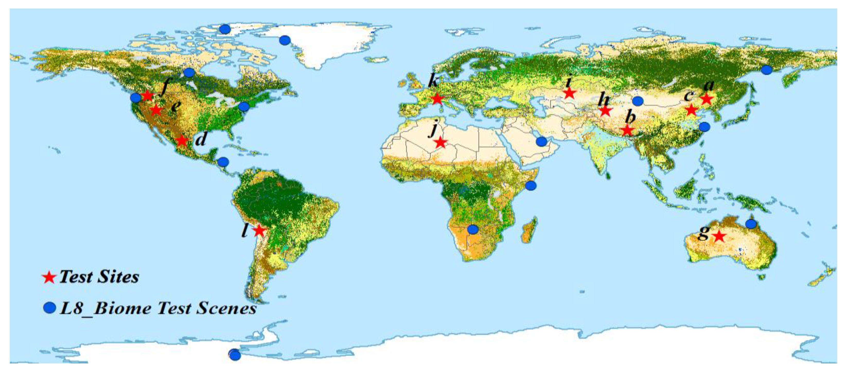
Twelve test sites (Figure 1), selected from areas where the problem of confusion between clouds and background surfaces is most severe, were chosen to evaluate the performance of the CECD for cloud detection. These sites were spread over six continents and covered a wide range of surface environments. For each test site, two scenes were randomly selected to test the performance of the CECD for Landsat-8 and Sentinel-2 data, respectively. These scenes included almost all possible seasons and surface-cover types, from desert to ice sheet. Details of the 24 test scenes are summarized in

Table 1. Details of the Landsat-8 and Sentinel-2 image scenes from the different test sites.

	Site	a	b	c	d	e	f
Landsat-8	Path row	p120r028	p139r039	p123r032	p029r043	p039r032	p043r027
	Date	2018/5/5	2019/2/22	2019/1/21	2018/9/9	2018/10/4	2018/5/25
	Confused types	BB, TC	SN, FW, BB	BI, FW, TC	BB	SN, FW, TC	TC
Sentinel-2	Granule tile	T51TXM	T45RWN	T50TMK	T13RGH	T11TQE	T11TMN
	Date	2019/5/4	2019/2/22	2019/8/13	2019/1/8	2019/1/11	2019/10/1
	Confused types	BB, TC	SN, BB, TC	BI, TC	BB, TC	SN, BB, TC	SN, BI, TC
	Site	g	h	i	j	k	l
Landsat-8	Path row	p106r075	p147r032	p159r026	p190r043	p195r028	p233r073
	Date	2018/12/2	2018/11/10	2018/7/24	2018/10/22	2018/10/9	2018/3/25
	Confused types	FW, BB, TC	SN, BD, TC	BB, FW	BD, TC	SN, BB, BI	FW, TC
Sentinel-2	Granule tile	T52KDB	T44TLL	T41UPP	T32RMN	T32TLS	T19KFV
	Date	2019/1/20	2019/2/14	2019/12/7	2019/10/18	2019/5/30	2019/12/10
	Confused types	BB, TC	SN, BB, TC	SN, BB, TC	BD, TC	SN, BI, TC	BB, FW, TC

Noted: TC., thin cloud; SN., snow; FW., frozen water; BB., bright bare lands; BI., bright impervious; BD., bright desert.

.

2.2. Datasets and Preprocessing

Due to its superiority in terms of spatial resolution (300 m) and revisit period (1–2 days) [40], Proba-V imagery was selected to generate cloud-free images. Proba-V was launched in 2013 and it has four optical spectral channels with wavelengths from 0.440 to 1.635 nm (

Table 2. The spectral bands of Landsat–8 and Sentinel-2 data used in this paper. The overlapping bands used for collecting training samples (Section 3.1) are highlighted in bold letters.

Band Names	Proba-V Bands (μm)	Landsat-8 Bands (μm)	Sentinel-2 Bands (μm)
Coastal	\	Band 1 (0.435–0.451)	Band 1 (0.433–0.453)
Blue	Blue (0.440–0.487)	Band 2 (0.452–0.512)	Band 2 (0.458–0.523)
Green	\	Band 3 (0.533–0.590)	Band 3 (0.543–0.578)
Red	Red (0.614–0.696)	Band 4 (0.636–0.673)	Band 4 (0.650–0.680)
Red Edge 1	\	\	Band 5 (0.698–0.713)
Red Edge 2	\	\	Band 6 (0.733–0.748)
Red Edge 3	\	\	Band 7 (0.765–0.785)
Wide NIR	NIR (0.772–0.902)	\	Band 8 (0.785–0.900)
Narrow NIR	\	Band 5 (0.851–0.879)	Band 8a (0.855–0.875)
Water vapor	\	\	Band 9 (0.930–0.950)
Cirrus	\	Band 9 (1.363–1.384)	Band 10 (1.365–1.385)
SWIR1	SWIR (1.570–1.635)	Band 6 (1.566–1.651)	Band 11 (1.565–1.655)
SWIR2	\	Band 7 (2.107–2.294)	Band 12 (2.100–2.280)

) [41]. Level 2A top-of-atmosphere (TOA) reflectance images were used in this study [40]. The clouds and shadows in the Proba-V images were masked based on the Proba-V quality band. Then, Proba-V images from within ± 15 days of the target date were used to produce a composite cloud-free image. The median composition method was used to generate the cloud-free image [42,43]. The median of all unmasked observations for each respective pixel was selected as the derived composite value.

Two types of widely used multispectral satellite data (Landsat-8, Sentinel-2) were selected to test the performance of the CECD. These data each have four spectral bands that overlap with those of the Proba-V satellite. Since most multispectral data do not include thermal infrared bands, and Joshi et al. [22] proved that clouds can be effectively detected without thermal bands, CECD uses only the top of atmosphere (TOA) reflectance bands ranging from the visible to short-wave infrared bands as inputs for each type of satellite image (Table 2). Because all the spectral bands in Landsat-8 data have a 30-m spatial resolution, the CECD will generate 30-m cloud masks for Landsat-8 data. For the Sentinel-2 satellite data, since they have three different spatial resolutions of 10, 20, and 60 m for different bands, in order to generate a uniform resolution cloud mask for Sentinel-2 imagery, the bands with 10 and 60 m spatial resolutions were resampled to 20 m. So, the cloud masks generated for Sentinel-2 images have a resolution of 20 m.

2.3. Validation Dataset

For each test scene, 800 samples were randomly selected. Because we only focused on the accuracy of the cloud detection, the samples were carefully labeled as belonging to one of two categories (cloud or clear) by checking the original satellite images. However, sometimes it is difficult to accurately interpret certain samples located at very thin clouds [14]. In order to ensure the reliability of each validation sample, the difficult-to-interpret samples were excluded from the evaluation process, and samples located at the intersection of clouds and land surfaces were moved to the interior of the relevant clouds. As a consequence, a total of 9362 Landsat-8 samples (3799 cloud samples, 5563 cloud-free samples) and 9341 Sentinel-2 samples (4085 cloud samples, 5256 cloud-free samples) were manually interpreted. To reduce the error in labeling [28], all the validation samples were collected and labeled by one particular scientist.

In order to objectively evaluate the robustness of our algorithm, we also selected some public cloud validation data from Landsat 8 Cloud Cover Assessment Validation Dataset (L8_Biome) (https://landsat.usgs.gov/landsat-8-cloud-coverassessment-validation-data) for independent testing. The L8_Biome was developed by Foga et al. [44], and each scene in the L8_Biome dataset has a manually labeled cloud mask. However, due to the low quality of some masks in L8_Biome, we did not use all the validation scenes in it. Since Li et al. [23] had screened out 19 high quality validation scenes from the L8_biome dataset through careful visual inspection, we chose the same scenes. In addition, because the Proba-V images were required in our calculation process, and they were only available after about November 2013 [41], the scenes before November 2013 were removed from the 19 validation scenes. Finally, a total of 14 L8_Biome scenes were selected for independent testing (Figure 1). The details of these scenes are listed in Table S1. Since there was no public cloud validation dataset for Sentinel-2 imagery, the independent validation part was only carried out on Landsat-8 images.

3. Method

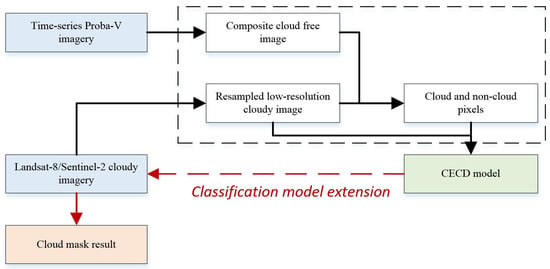
The CECD method is designed for masking clouds in images acquired by different medium-resolution optical sensors, and does not require thermal infrared bands. The method consists of three main parts: first, the medium-resolution cloudy image is resampled to a low-resolution one and, together with a composited low-resolution cloud-free image, is used to identify cloud and non-cloud pixels. Secondly, using the identified cloud, non-cloud pixels and the resampled cloudy image, training samples are automatically collected to develop a local adaptive classification model at a low-resolution level for each scene. Finally, the trained classifier is extended to mask clouds in the corresponding medium-resolution image. In our particular case, the composited low-resolution cloud-free image was derived from Proba-V data, and the medium-resolution cloudy images were Landsat-8 and Sentinel-2 images. A flowchart of CECD method is illustrated in Figure 2.

3.1. Identifying Cloud and Non-Cloud Pixels with the Support of Reference Cloud-Free Imagery

Our aim is to collect training samples at a low-resolution level. However, distinguishing pixels between bright surfaces and clouds and the detection of thin clouds are the two main obstacles in identifying cloud and non-cloud pixels [12,18]. In order to collect accurate training samples, the medium-resolution cloudy Landsat-8 and Sentinel-2 images were aggregated to the Proba-V resolution to work with the composited cloud-free Proba-V images (see Section 2.2) to figure out these problems.

First, as bright surfaces can be well separated from clouds with the help of a corresponding cloud-free image [16,17], the composited cloud-free Proba-V images and the resampled Landsat-8 and Sentinel-2 cloudy images were used to enhance the difference between clouds and bright surfaces. A temporal haze optimized transformation (THOT) method, which was not sensitive to the errors caused by inconsistencies in reflectance between cloud-free and cloudy images [16], was used for this (Equation (1)).

$$THOT={\displaystyle \sum }_{i=1}^n{k}_i\Delta R_i+c$$

(1)

where $\Delta R_i$ is the difference in reflectance between the cloudy and cloud-free images for an overlapping band $i$ for a given pixel. The bands used to calculate $\Delta R$ in this study are highlighted in bold in Table 2. $n$ is the number of overlapping bands; $k_i$ and $\mathrm{c}$ are coefficients determined by a multivariate regression between the haze optimized transformation (HOT) and $\Delta R_i$:

$$HOT={\displaystyle \sum }_{i=1}^n{k}_i\Delta R_i+c+\epsilon ,whereHOT=sin\theta \ast R_{blue}-cos\theta \ast R_{red}$$

(2)

where $\epsilon$ is the regression residual, and $R_{blue}$ and $R_{red}$ are reflectances at the TOA of the blue and red bands in the cloudy image, respectively. $\theta$ is the angle of the “clear line” of the corresponding cloud-free image, and the “clear line” can be fitted by a line regression of the blue and red bands in the cloud-free image [45]. Since $\Delta R_i$ for non-cloudy pixels is close to zero and smaller than for cloudy ones, the THOT index, which is the linear sum of $\Delta R_i$ (Equation (1)), can separate clouds from bright surfaces well [16].

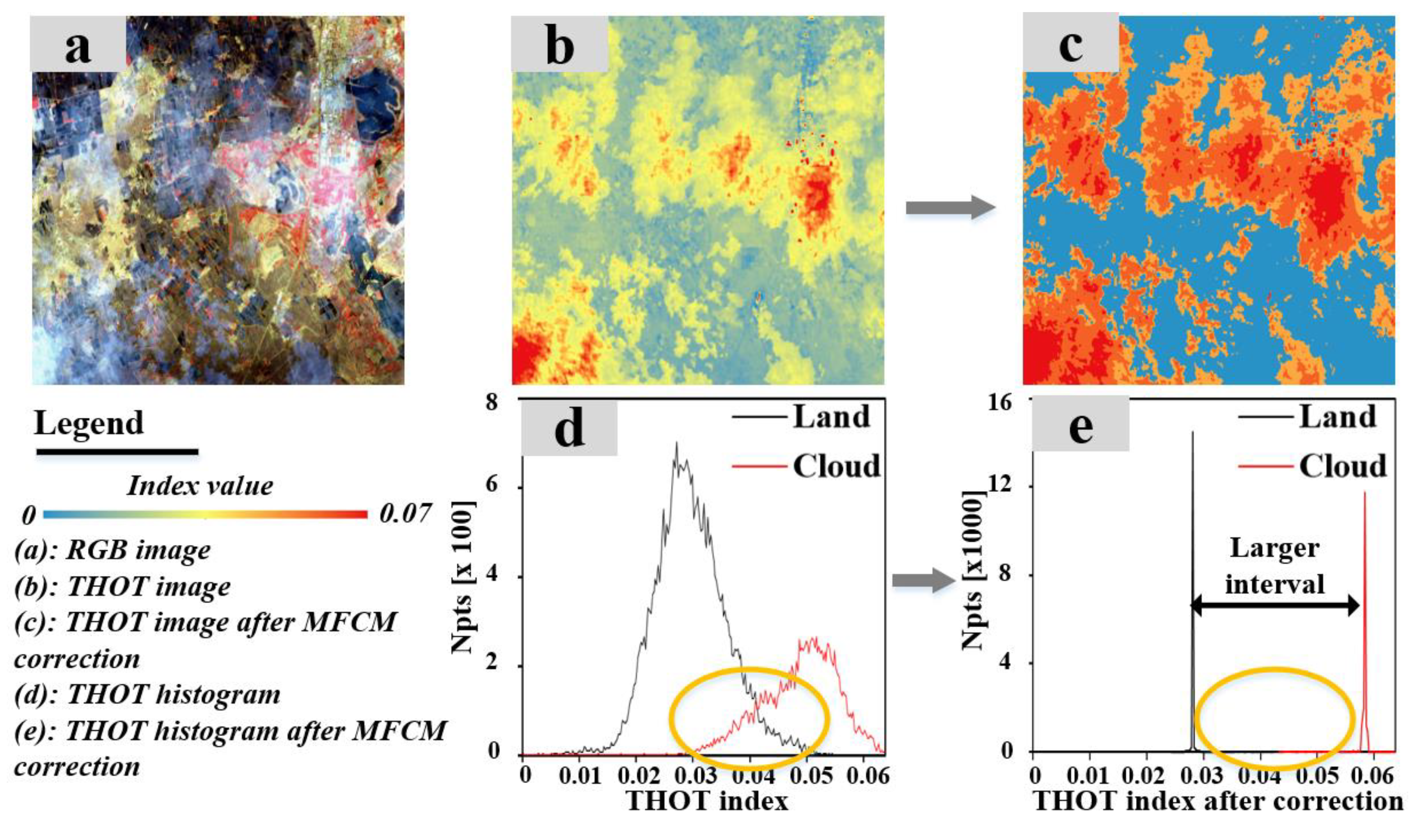
Secondly, since the combination of the fuzzy C-means (FCM) algorithm and local information could fully compensate for the poor spectral contrast of the mixed pixels [46], a modified fuzzy C-means (MFCM) method [47] was applied to the generated THOT image to further enhance the contrast between thin clouds and adjacent non-cloud pixels (Equation (3)). By minimizing the objective function, J, a corrected THOT value, x, was derived (the complete calculation process is presented in the Appendix A).

$$J={\displaystyle \sum }_{i=1}^c{\displaystyle \sum }_{j=1}^N{\mu }_{ij}^m{\left(x_j-v_i\right)}^2+a{\displaystyle \sum }_{i=1}^c{\displaystyle \sum }_{j=1}^N{\mu }_{ij}^m{\left(\overline{x_j}-v_i\right)}^2,x_j=THO{T}_j-{\beta }_j$$

(3)

where ${\mu }_{ij}^m$ is the probability that a pixel $j$ belongs to cluster $i$; m is a weighting exponent, for which a default value of 2 was used; $x_j$ is the corrected THOT value of pixel $j$ obtained by subtracting the gain field, ${\beta }_j$; $N$ is the total number of pixels; C is the number of clusters, which was set to 2 (cloud and non-cloud); $v_i$ is the prototype of the centroid for cluster $i$; $\overline{x_j}$ is the mean value of the pixels within a 3 × 3 window around pixel j; and $a$ controls the neighboring effect—a default value of 0.3 was used for this. Since Yang et al. [47] conducted comprehensive tests on these parameters, and the default values of all parameters were the optimal values they derived, all the parameters in MFCM were set as the default settings. An example of the application of this method to a HOT image histogram is shown in Figure 3 below. It polarizes the image reflectance distribution of clouds and lands to generate a dual-mode histogram (Figure 3e), which results in an increase in the contrast between thin clouds and neighboring surfaces in the corrected image (Figure 3c).

Finally, as the contrast between surfaces and clouds was effectively enhanced, it was reasonable to draw a conclusion that accurate cloud and non-cloud pixels could be easily identified by using an appropriate threshold. A simple automatic thresholding method, OTSU, proposed by Otsu [48], was then applied to the corrected THOT image to identify cloud and non-cloud pixels.

3.2. Classification Extention-Based Cloud Detection Model

3.2.1. Collection of Training Samples

The training samples were automatically collected using the identified cloud and non-cloud pixels (see Section 3.1) and the blue band of the resampled low-resolution Landsat-8 and Sentinel-2 cloudy image. As the reliability and representativeness of the training samples directly affect the accuracy of classification, a bin-based sample selecting approach proposed by Zhu et al. [1] was employed to search for representative cloud and non-cloud samples with different brightnesses. We first divided the 0–1.0 range of the blue reflectance values in the resampled cloudy image into 5 bins with equal intervals. Then, each bin was divided into cloud and non-cloud sub-bins based on the identified cloud and non-cloud pixels, and the erosion operator [49] was used to remove the “salt-and-pepper” pixels in each sub-bin. Finally, training samples of clouds and non-cloud surfaces were derived from the remaining pixels in each sub-bin. In order to optimize the distribution of the samples, samples were collected from sub-bins in proportion to the area occupied by each sub-bin [50,51].

3.2.2. Modeling of Random Forest Classifier

As a local adaptive classification model can achieve a higher classification accuracy than a single global model [52], a local adaptive model was developed for each scene based on the collected training samples from that scene (Section 3.2.1). First, the spectral data of the training samples in the resampled low-resolution Landsat-8 and Sentinel-2 image were extracted to build the training data. Due to the complex spectral characteristics of clouds and surface objects, objects can exhibit similar spectral behavior to clouds in certain spectral bands [32]. It is a challenge to accurately detect clouds using a limited number of spectral bands [23]. Therefore, in order to make full use of the spectral information, all Landsat-8 and Sentinel-2 bands mentioned in Table 2 were used. Then, a local adaptive classification model was trained using the training data derived from the low-resolution Landsat-8 and Sentinel-2 image. It should be noted that, since our method is a local adaptive classification method, it is not sensitive to radiometric and reflectance calibration [53]. Therefore, both top-of-atmosphere and surface reflectance data can be used for model training. Finally, the modelled classifier was extended to the original medium-resolution Landsat-8 and Sentinel-2 image to classify cloudy pixels.

According to the previous investigations [37,52], the RF classifier is capable of processing highly dimensional multicollinear data, and rarely affected by noise and feature selection. In addition, it proves to be more accurate and efficient than other widely used classifiers such as the support vector machine (SVM), artificial neural network (ANN), and classification and regression tree (CART) classifiers [54,55,56,57,58]. Considering the advantages of RF classifier, it was employed in this study. The RF classifier has two parameters: the number of classification trees (Ntree) and the number of selected predication features (Mtry). Since many researchers have demonstrated that there is almost no correlation between these two parameters and the classification accuracy [54], a value of 100 for Ntree and the square root of the total number of training features for Mtry were selected.

4. Results and Accuracy Assessment

4.1. Performance of CECD Using the Landsat-8 and Sentinel-2 Imagery

4.1.1. Cloud Masking in Landsat Imagery

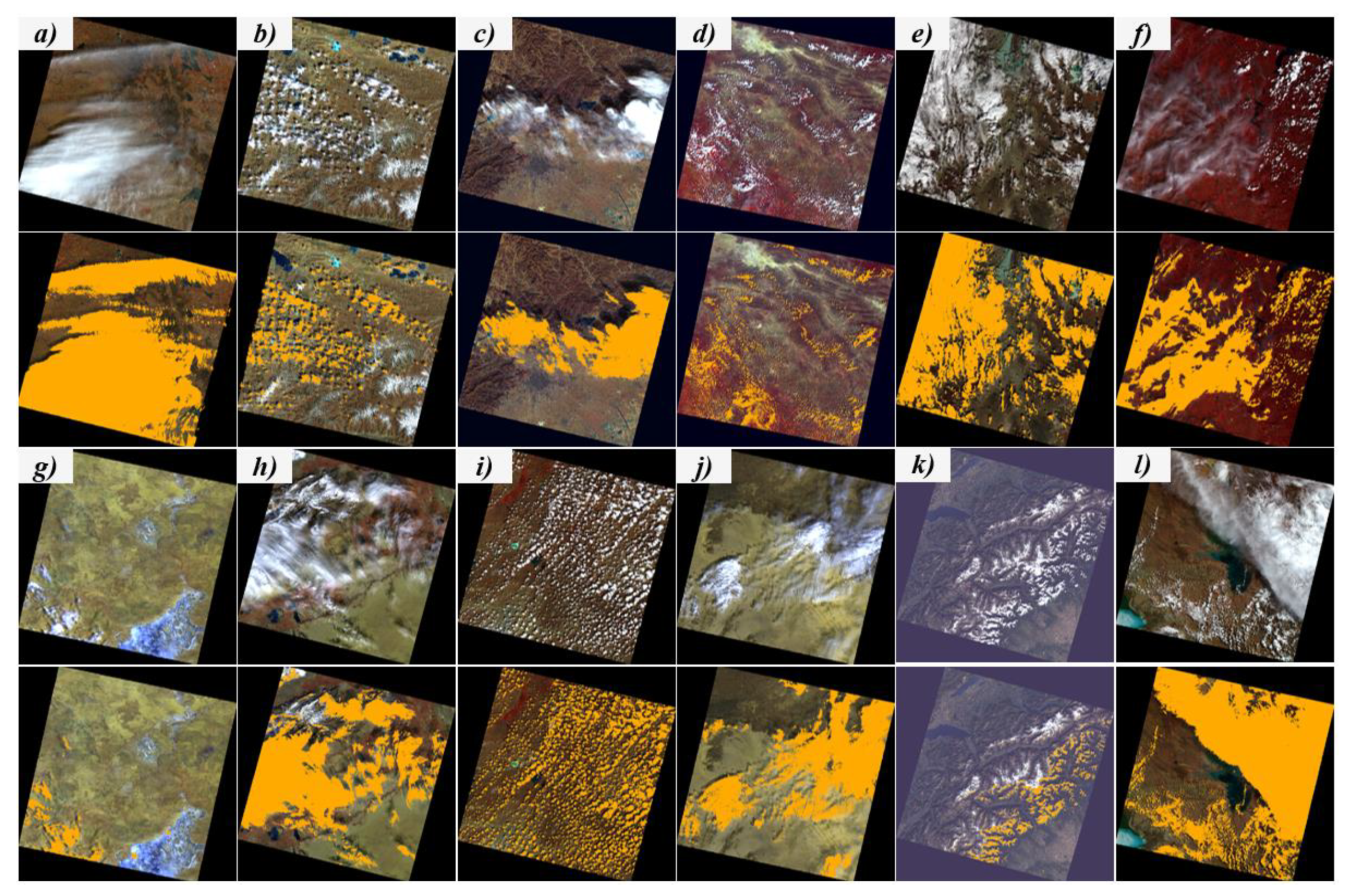
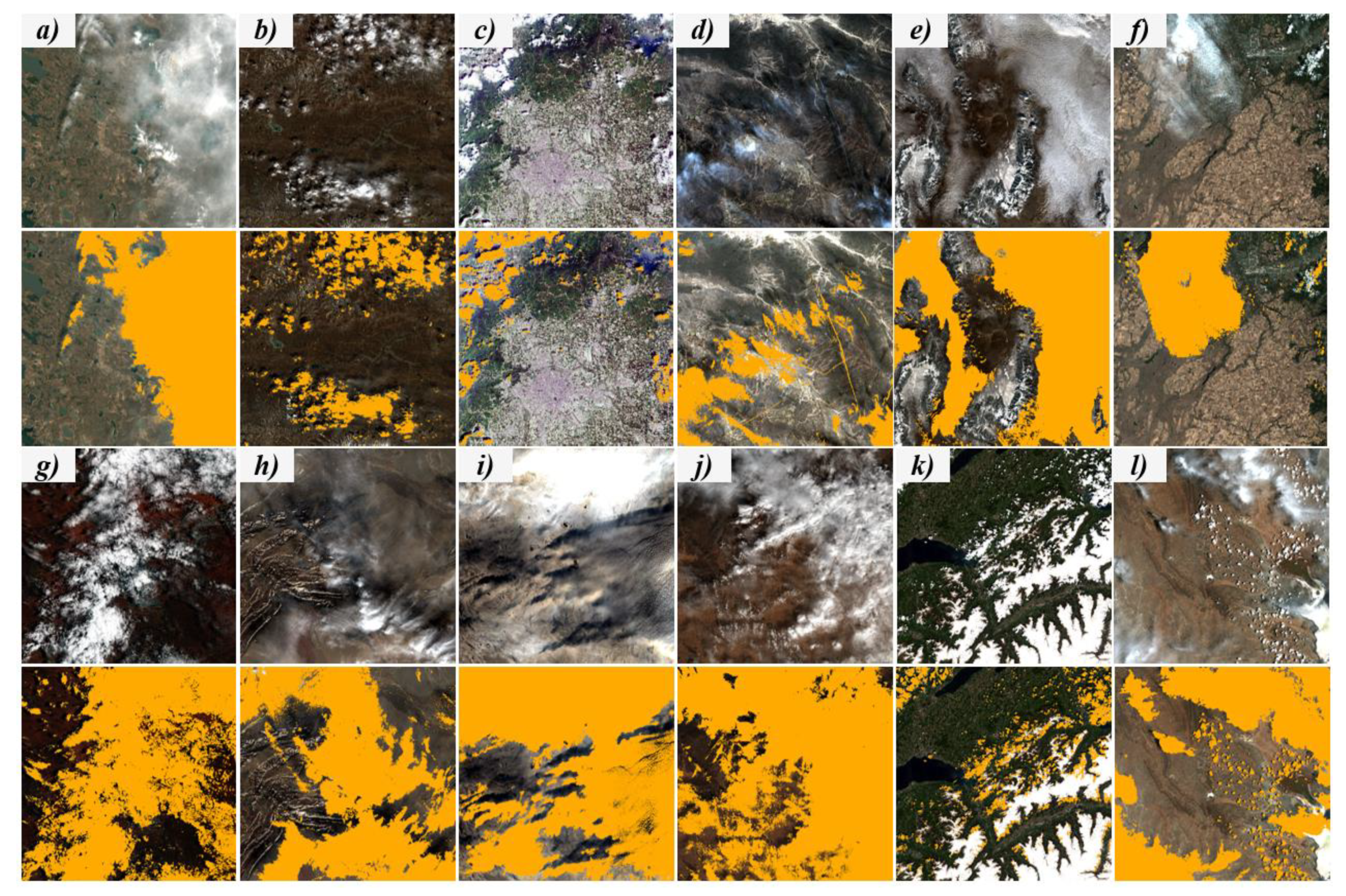
The cloud-detection results for the 12 Landsat-8 test scenes are illustrated in Figure 4: it can be seen that there is significant agreement between the CECD cloud cover and the actual cloud distribution. All kinds of cloud-contaminated pixels, including thick and thin clouds, are accurately separated from snow, bright sand, bright impervious surfaces and bright rocks—surfaces that are usually confused with clouds using traditional methods. Therefore, the proposed CECD can effectively extract clouds and mitigate the disturbances caused by other bright land surfaces with similar spectral reflectance. For example, a large proportion of snow, bright bare lands, and bright impervious surfaces are shown in Figure 4b–e,g,h,k, but there is no overestimation of clouds in the corresponding CECD results. Moreover, the thin clouds over different land-cover types are also accurately captured in the detection results (Figure 4a,c,f,j,l). It can be observed that the details of the cloud boundaries and internal structures are well described in our cloud-mask maps, which further reveals the effectiveness of the proposed CECD.

4.1.2. Cloud Masking in Sentinel-2 Imagery

The second experiment was conducted on the 12 Sentinel-2 test images, and the corresponding cloud-detection results are given in Figure 5. Unlike for Landsat-8 imagery, due to the lack of thermal bands, the separation between clouds and other bright surfaces is always a big problem when using conventional automated cloud-detection methods for Sentinel-2 images [12,14]. However, this issue can be greatly alleviated by using CECD (Figure 5). Both thick and thin clouds are well separated from the bright surfaces in the results shown. For instance, the scenes in Figure 5b,d,e,h–k are very complex cases containing snow, bright bare lands, and bright rocks. The cloud pixels are also well identified in the corresponding CECD cloud masks. In addition, the low-altitude thin clouds that are usually underestimated by traditional cloud-detection methods are also effectively detected by the CECD cloud masks (Figure 5a,d,f–j,l). Therefore, it can be said that the CECD method can also achieve a reasonably good performance when applied to Sentinel-2 images without using the thermal infrared bands.

4.2. Comparison with FMASK Cloud-Detection Algorithm

The CECD was compared with the function of mask (FMASK) algorithm for the 24 Landsat-8 and Sentine-2 test scenes (see Section 2.1). FMASK is a cloud-mask algorithm that was designed for masking clouds in Landsat and Sentinel-2 imagery, and it was the operational method used for Landsat data products [11]. The latest FMASK version, FMASK 4.0 [14] (https://github.com/gersl/fmask), which is the state-of-the-art FMASK cloud detection technique, was used for comparison with the CECD. In order to ensure the objectivity of the comparison, the dilation parameter in FMASK was set to 0 to be consistent with the CECD. Except for this, because the default values of all other parameters in FMASK are the optimal thresholds obtained by performing sensitivity analysis using images in different environments around the world [14], these default thresholds are applicable to different types of clouds and different regions. Therefore, all the other parameters in FMASK were set to the default parameter settings described in Qiu et al. (2019).

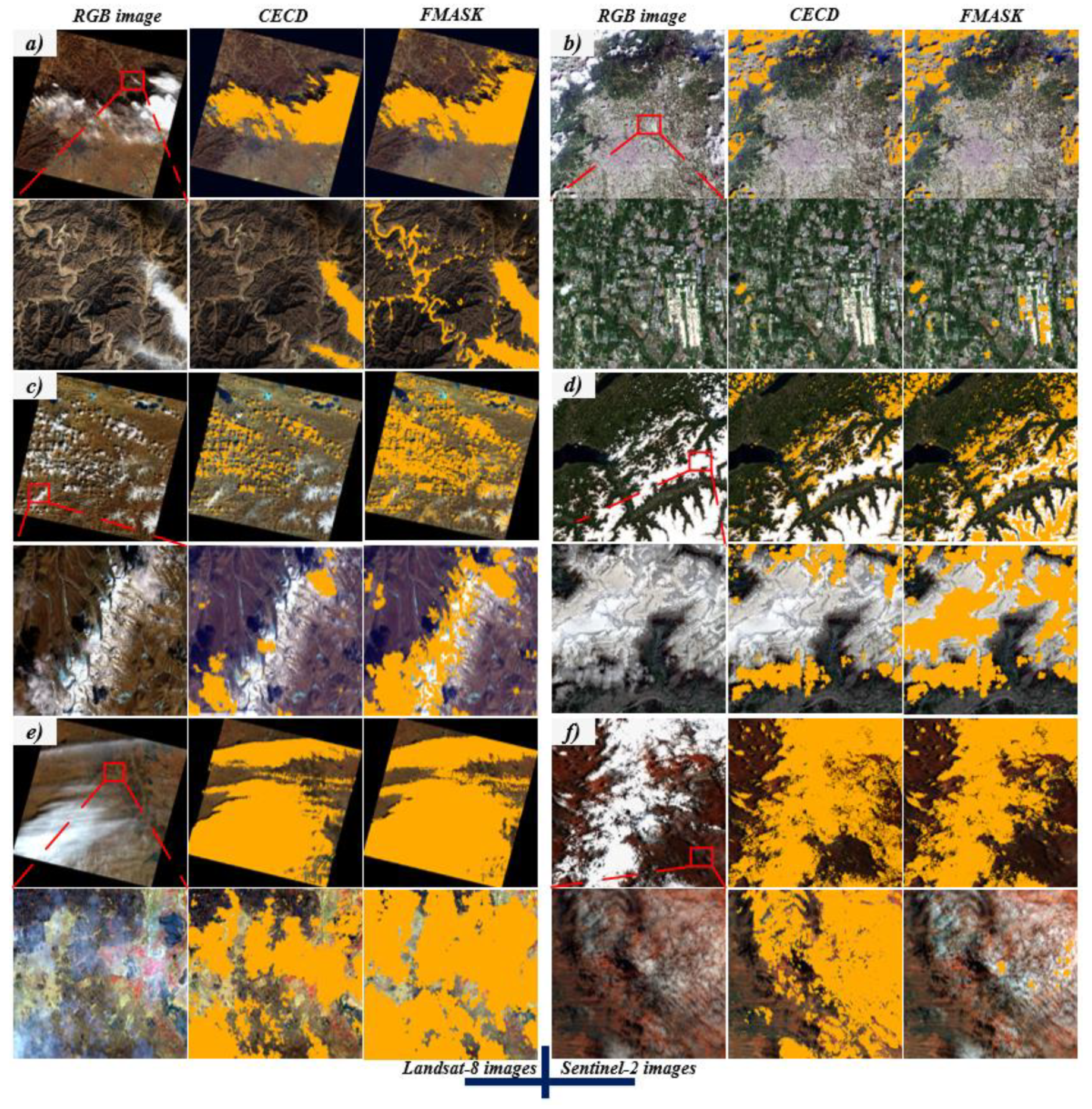
To quantitatively evaluate the accuracy of the results, three traditional metrics [59] including the user accuracy (U.A.), producer accuracy (P.A.), and kappa coefficient (K.C.) were calculated using the validation samples independently selected from each test scene (Section 2.3). In addition, the F-measure (F.M.), which is a single class-specific accuracy metric and the complement of the commission, omission, and overall error, was also calculated using a balanced weighting (β = 1) [22,60,61].

Table 3. Accuracy assessment results for CECD and function of mask (FMASK) based on the application of these methods to the Landsat-8 and Sentinel-2 scenes at the 12 test sites [%].

			a	b	c	d	e	f	g	h	i	j	k	l	A. A.
Landsat 8	Npts	C. S.	545	244	253	164	420	357	83	423	274	417	125	494	/
		N. S.	235	537	507	578	340	426	705	331	505	470	647	282	/
	CECD	P. C.	95.91	95.27	97.86	98.75	96.18	97.66	96.97	96.41	98.72	97.18	97.43	95.33	96.88
		U. C.	99.51	96.48	99.59	95.33	99.75	98.88	99.98	98.90	99.53	98.01	99.63	99.89	98.64
		P. N.	99.74	98.31	99.79	97.92	99.51	98.23	99.95	98.91	99.77	96.89	99.98	99.17	98.11
		U. N.	98.26	97.21	97.29	98.55	93.61	93.28	98.47	96.23	97.94	92.59	98.07	94.05	96.67
		F. M.	97.86	95.75	98.71	95.84	97.85	97.77	98.25	97.75	99.14	96.85	98.65	97.37	97.65
		K. C.	95.75	93.12	95.69	92.86	94.64	92.94	98.31	95.49	96.56	91.26	94.55	91.51	94.33
	FMASK	P. C.	98.86	99.62	99.60	98.48	98.04	89.25	90.22	97.92	99.03	94.39	98.79	96.42	97.06
		U. C.	97.65	59.18	78.14	92.06	93.64	99.99	99.97	82.38	99.10	98.58	60.31	88.71	87.47
		P. N.	94.59	66.17	85.60	97.46	87.89	99.99	99.97	79.19	99.53	97.93	86.62	80.61	89.62
		U. N.	99.99	99.72	99.76	99.26	99.29	90.04	98.22	97.68	99.07	92.14	99.29	93.12	97.29
		F. M.	98.27	72.70	87.19	94.95	94.34	94.31	94.73	91.43	99.08	95.96	73.71	92.94	90.80
		K. C.	96.04	56.06	76.98	92.04	90.36	83.15	88.17	79.34	97.35	90.90	65.82	78.52	82.88
Sentinel-2	Npts	C. S.	441	272	143	203	408	186;	523	383	490	637	167	232	/
		N. S.	339	518	649	571	369	610	268	385	218	138	634	557	/
	CECD	P. C.	96.00	95.27	95.01	96.63	96.24	97.93	98.07	97.65	97.39	97.03	96.22	96.19	96.46
		U. C.	99.76	96.48	95.00	98.41	94.25	99.46	98.28	95.41	94.38	99.82	98.59	99.67	97.46
		P. N.	99.71	98.31	98.94	99.47	93.67	99.84	97.11	94.93	91.90	98.89	99.69	99.46	97.66
		U. N.	95.08	97.21	98.49	97.09	95.85	99.67	96.76	97.40	99.10	89.03	99.37	95.9	96.66
		F. M.	97.85	96.00	95.10	97.55	95.30	98.69	98.29	96.33	96.91	98.37	97.49	97.41	97.11
		K. C.	95.15	93.12	92.71	97.41	89.99	98.94	95.11	92.67	92.19	92.60	97.41	92.81	94.18
	FMASK	P. C.	98.99	98.62	93.01	97.12	97.07	99.47	84.37	97.18	87.35	93.96	97.96	98.09	95.01
		U. C.	92.41	59.18	74.70	99.47	82.82	97.82	99.76	73.54	73.67	99.64	61.57	92.13	83.81
		P. N.	89.68	66.17	91.55	99.82	78.73	99.35	99.64	57.10	57.26	97.78	86.62	93.20	84.74
		U. N.	98.86	98.72	98.42	97.26	93.67	99.84	78.39	92.35	76.78	83.81	99.48	96.64	92.36
		F. M.	95.68	74.98	80.40	98.29	89.75	98.68	91.43	80.88	84.66	96.65	78.76	91.50	88.47
		K. C.	90.63	56.06	72.73	97.80	74.24	98.26	79.11	55.32	43.54	88.55	67.19	88.97	76.03

Noted: Npts., number of sample pixels; C. S., cloud samples; N. S., non-cloud samples; P. C., producer’s accuracy of cloud; U. C., user’s accuracy of cloud; P. N., producer’s accuracy of non-cloud; U. N., user’s accuracy of non-cloud; F. M., F-measure; K. C., kappa coefficient; A. A., averaged accuracy.

summarizes the quantitative accuracy results, and Figure 6 illustrates a comparison between the cloud-detection results produced by CECD and FMASK for three typical Landsat-8 scenes and three Sentinel-2 scenes. As shown in Table 3 and Figure 6, for both algorithms, the overall accuracy was high for most of the test scenes. However, CECD produced a more robust performance than FMASK in the case of both Landsat-8 and Sentinel-2 images. The average F-measure value for CECD was 97.65% and 97.11% for Landsat-8 and Sentinel-2, respectively. In comparison, FMASK gave an average F-measure value of 90.80% and 88.47% for the Landsat-8 and Sentinel-2 imagery, respectively. FMASK did not perform as well with the Sentinel-2 dataset as it did with the Landsat-8 imagery. For instance, it can be observed that FMASK omits many low-altitude clouds in the corresponding Sentinel-2 cloud mask (Figure 6f), while even the very thin clouds are well depicted in the Landsat-8 classification results (Figure 6e). Without thermal bands, it is problematic for FMASK to detect low-altitude thin clouds. Moreover, for scenes containing a large amount of snow/ice and bright impervious surfaces (Landsat-8 scenes at site b, c, h, k, and l; Sentinel-2 scenes at site b, c, e, h, i, and k), the accuracy of FMASK is much less than that of CECD (average F-measure value of CECD is 97.65% and 96.19% as against 83.59% and 81.57% for FMASK for the Landsat-8 and Sentinel-2 images, respectively). As clearly illustrated by Figure 6a–d, there is noticeable misclassification by the FMASK method in these scenes. A large number of bright surfaces are mistakenly labeled as clouds in the FMASK results, whereas the CECD performs well for these scenes.

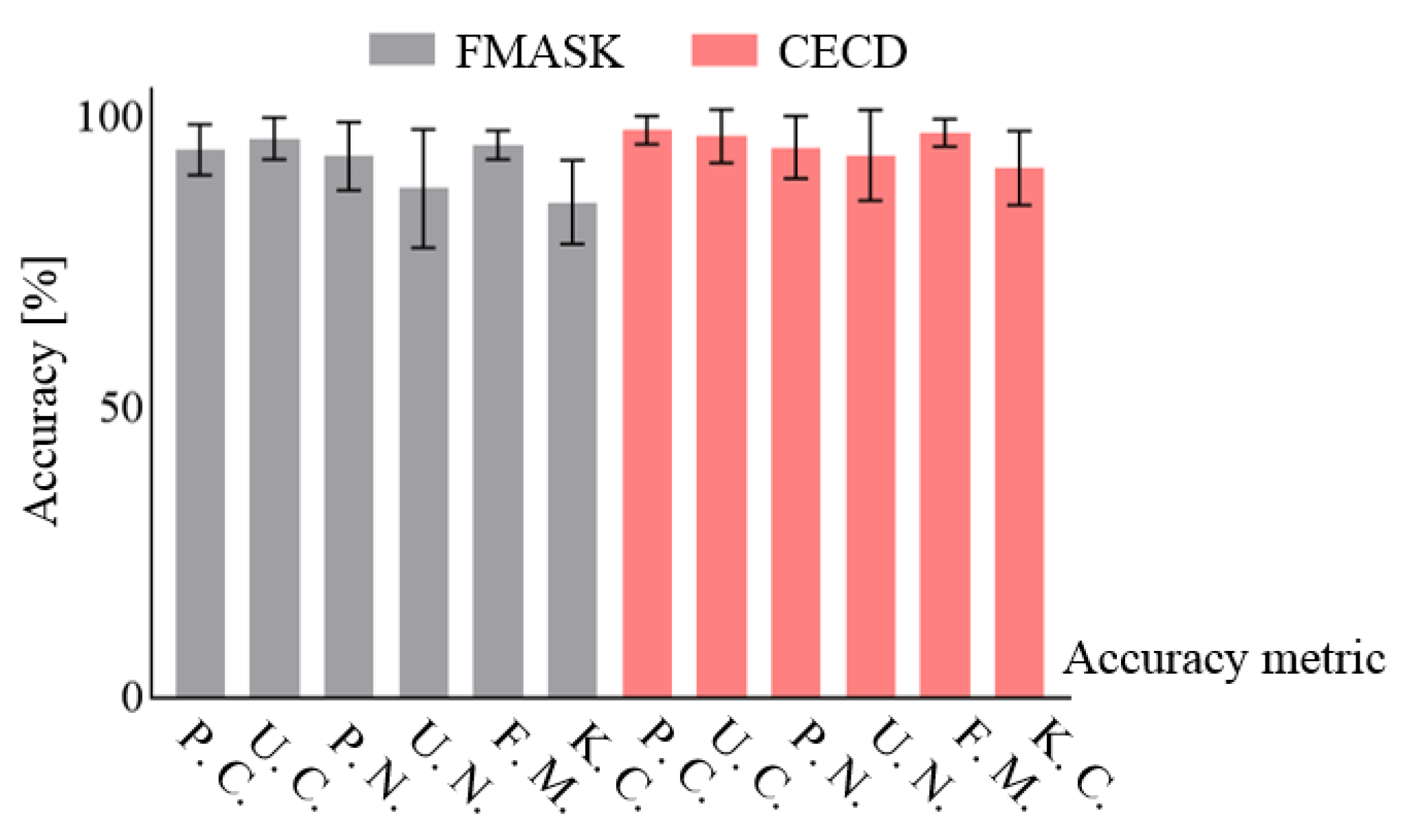
To comprehensively evaluate the performance of FMASK and CECD in relation to specific surface cover types, the pixels in the 24 test scenes (Table 1) were visually classified as vegetation, bare land, impervious, snow/ice, or water classes based on their spectral characteristics. The average cloud-detection accuracies of the two algorithms for these surface covers were calculated and shown in Figure 7. The robust non-parametric McNemar’s statistics (chi-square (χ²) and 95% confidence interval probability) [62] were calculated to evaluate the statistical significance of differences (refer

Table 4. McNemar’s test for the difference between the results for the FMASK and CECD cloud masks for specific environments.

		Vegetation	Water	Barren	Impervious	Snow
Landsat-8	χ2	0.36	2.44	3.23	54.39	215.43
	p-value	0.55	0.11	0.07	0.00	0.00
Sentinel-2	χ2	0.13	1.12	17.06	60.01	232.07
	p-value	0.72	0.28	0.00	0.00	0.00

). Note that only when p < 0.05 and χ² > 3.841 does it indicate a statistically significant change, and all these accuracy metrics were derived using a sample set aggregated from the 24 selected test scenes (Table 1). The two sets of results show the highest statistically significant differences in the snow/ice, followed by the impervious regions. As for barren lands, the cloud detection of the two methods was significantly different in the Sentinel-2 images, but there is no noticeable advantage at the chi-square and the 95% significance level in the Landsat-8 scenes. Moreover, the performance of CECD was comparable to that of FMASK in the water and vegetation areas. These difference were also notable in the accuracy assessment of Figure 7. Compared with FMASK, the CECD results show a significant improvement for the snow/ice-covered regions in the Landsat-8 (F-measure of 96% against 88%) and Sentinel-2 images (F-measure of 95% against 82%), and impervious areas were also improved (F-measure of 96% against 90% for Landsat-8, and 97% against 85% for Sentinel-2). In addition, the improvement of CECD for the Sentinel-2 images was higher than that for the Landsat-8 images in the barren land surfaces. Furthermore, both FMASK and CECD produced good results for areas of both vegetation and water.

An independent validation experiment was performed using the 14 Landsat-8 images selected from the L8_Biome dataset (Figure 1). All the non-cloud classes (clear and cloud shadow) in the reference mask of each image were merged into the non-cloud class, and the cloud classes (cloud and thin cloud) were aggregated to the cloud class. These processed cloud masks were used as ground truth to compare the robustness of CECD and FMASK (Figure 8). It can be seen from the results that the accuracy of CECD and FMASK are both high in these scenes, and the accuracy of CECD is higher than that of FMASK (F-measure value of 96.95% against 93.45%). Moreover, the standard deviation error of CECD on each accuracy metric is less than that of FMASK. Therefore, according to all results in Figure 6, Figure 7 and Figure 8, and the accuracy assessment in Table 3 and Table 4, it can be concluded that our CECD method is a robust cloud detection method.

5. Discussion

5.1. Effectivenss of Classification Extention Strategy in Cloud Detection

Zhang et al. [36] proposed a classification extension strategy for land cover mapping. They developed local adaptive classifiers using the 500 m resolution MODIS surface reflectance dataset and extended them to classify the corresponding 30 m Landsat surface reflectance images. This strategy is able to overcome the difficulty of collecting training samples in large-scale land cover mapping [36]. However, it was based on the assumption that the two different remote sensing datasets have highly consistent spectral reflectance. In this study, the training spectral data were derived from the resampled Landsat-8 and Sentinel-2 images, and the target datasets for model extension were the original medium-resolution Landsat-8 and Sentinel-2 datasets themselves. Therefore, except for the errors caused by resampling, the spectral signatures used for training were basically the same as those of target datasets. All selected Landsat-8 images (Table 1) were used as a case to illustrate the consistency between the original medium-resolution TOA reflectance and the resampled 300 m low-resolution TOA reflectance (Figure 9). As shown in Figure 9, all eight bands of the original Landsat-8 OLI data were in a good agreement with the resampled ones, and the average coefficient of determination (R²) and the root mean square error (RMSE) of all bands are higher than 0.88 and less than 0.053, respectively. Similarly, Li et al. [23] found that the model trained at a resolution 10 times lower than the spatial resolution of the target image could still be effectively used to detect clouds of the original target image. Therefore, the classification extension-based cloud detection method can be considered as a suitable method for classifying cloudy pixels of medium-resolution optical images.

5.2. Reliability of the Collected Training Samples

In this study, we used the THOT and the MFCM methods to separate clouds from background surfaces to obtain accurate training samples. The THOT method was used to enhance the difference between clouds and bright surfaces, and the MFCM method was to highlight the features of thin cloud pixels. Because the reliability of training samples is directly related to the accuracy of classification [63], it is also very important to evaluate the accuracy (proportion of correct samples) of training samples. Generally, evaluating the accuracy of all training samples is difficult and time-consuming. Fortunately, since each scene in the L8_Biome dataset has a manually labeled cloud mask, we measured the reliability of the training samples in Landsat-8 imagery by comparing the training samples collected in the 14 selected L8_Biome images with their corresponding cloud masks. We found that these training samples achieved overall accuracies of 96.97% and 93.58% for clouds and non-cloud surfaces in the Landsat-8 scenes, respectively. In addition, since there were no available cloud masks for Sentinel-2 imagery, the accuracy of training samples in Sentinel-2 images was validated by visual inspection. We randomly selected 200 training samples from each Sentinel-2 test scene (Table 1), and visually checked the correctness of the samples based on the original images. The overall accuracies were 97.6% and 94.5% in the Sentinel-2 scenes for clouds and non-cloud samples, respectively. Although the training samples still contained a small number of erroneous points, the random forest model was demonstrated to be resistant to noise and the presence of erroneous samples [54]. Meanwhile, Gong et al. [64] found that the decrease in overall accuracy of RF classifier was less than 1% when the error in the training samples was less than 20%. Therefore, the training samples derived in this study were accurate enough for use in detecting cloud pixels.

5.3. Computational Efficiency

In order to comprehensively analyze the efficiency of our algorithm, we took the 12 Landsat-8 test scenes (Table 1) as an example and compared the CECD with two other popular cloud detection approaches: the rule-based approach and the operational single classifier-based machine learning approach (classify images using a single global classifier) (Figure 10). The FMASK 4.0 was used as a rule-based example, and the single classifier-based machine learning (hereafter SCML) approach was realized by using a single RF classifier trained from all validation samples (Section 2.3). Considering that the FMASK method included the process of cloud shadow detection, in order to ensure the objectivity of the comparison, the time consumed by the cloud shadow detection in FMASK was excluded. The hardware environment of our test was: CPU: i7-4720HQ on a 2.6 GHZ, RAM: 16GB.

From Figure 10, we could see that the computational efficiency of the machine learning-based methods of CECD and SCML was more stable than the rule-based FMASK 4.0 method. The time required for CECD and SCML to calculate a Landsat image was about 4.3 min, while FMASK took 2 to 5 min for different scenes. Since the efficiency of FMASK depends on the size and complexity of images [14], the time FMASK spent on different images varied greatly. In addition, since our CECD method trained local adaptive classifiers at a low-resolution scale (300 m), the time cost of training was relatively small for each scene (about 5 s), and thus the efficiency of our method was very close to that of using a single global classifier. Therefore, our CECD algorithm can be regarded as suitable as an operational method.

5.4. The Importance of Input Features for Different Environments

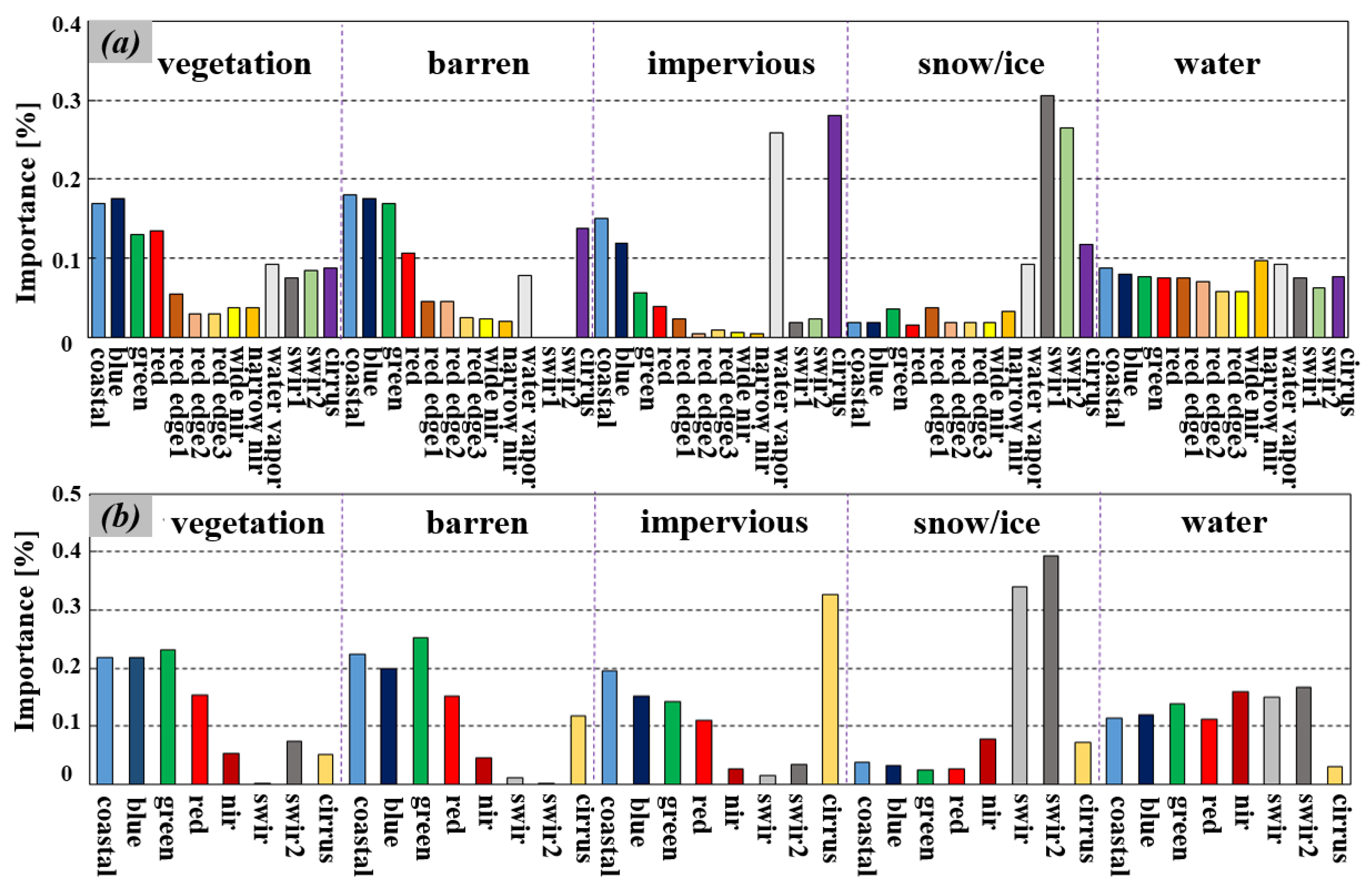
In this paper, we trained the CECD model using all optical bands of Landsat-8 and Sentinel-2 imagery (Table 2). However, it is also important to evaluate the need to use multi-spectral information for cloud masking. To quantify the importance of each band for cloud detection in different environments, the 24 test scenes (see Table 1) were visually classified into five landscapes: vegetation, bare land, impervious, snow/ice, and water. Since the RF model can measure the importance of a variable by calculating ‘out-of-bag’ data for the variable while keeping all the other variables constant [65], this operation was carried out using the RF model, and the results were obtained using all samples from the 24 selected scenes, as shown in Figure 11.

The results indicate that the coastal and visible bands contributed the most to mask clouds over vegetation and barren land surfaces. Meanwhile, the cirrus band of Landsat-8 and the water vapor and cirrus bands in Sentinel-2 images also had a great contribution to cloud detection over barren land surfaces. In addition, as for cloud detection over the impervious regions, the two water vapor absorption bands (940 nm water vapor band and 1380 nm cirrus band) in Sentinel-2 imagery were found to be the most important features, followed by the coastal and blue bands. In comparison, the coastal, visible, and cirrus bands had the greatest contribution to cloud detection over impervious areas in Landsat-8 images. Moreover, when detecting clouds over snow/ice areas, the SWIR bands had been shown to be the most important for Sentinel-2 and Landsat-8 imagery. As for water regions, except for the cirrus band, the importance of other bands was basically the same in the Landsat-8 imagery, and the NIR and SWIR2 bands had the greatest contribution. Similarly, it was found that the contribution of each Sentinel-2 band was also not much different when detecting clouds over water, and the NIR and water vapor bands were shown to be the most important features. Due to the different importance of each band in different environments, it is necessary to make full use of spectral information when masking clouds in complex landscapes.

5.5. Limitations of the Use of CECD for Cloud Detection

Firstly, to produce a composite cloud-free image, multi-temporal low-resolution images are needed. Fortunately, there are already some composited cloud-free low-resolution datasets available that can be used directly, such as MOD09A1. In addition, with the advent of the Google Earth Engine (GEE) platform, the requirements for compositing cloud-free images can easily be met by using the free-access GEE cloud-computation platform [66].

Secondly, although our proposed CECD can easily be adapted for use with different sensors, it may fail in some complex scenes for imagery with only visible and near-infrared reflectance channels, as the SWIR bands are crucial for distinguishing the snow/ice class from clouds [11,30]. Therefore, in the absence of SWIR bands, the CECD may give a reduced accuracy in high-altitude snow-covered regions. Due to the limited number of features that can be used to discriminate between classes and the similar spectral reflectance, snow/ice pixels are often confused with clouds in the visible and near-infrared bands.

Thirdly, although the classifier derived from the resampled low-resolution Landsat-8 and Sentinel-2 images was successfully used to classify clouds in the corresponding 30 m and 20 m images, this classifier may not be suitable for classifying clouds in images with very high spatial resolutions (such as images with a resolution higher than 5 m). Dorji et al. [67] evaluated the impact of different spatial resolution images on the observation results, and found that the characteristics of the object in the image with a resolution of 2 m are completely different from the characteristics in the image with 1 km resolution. When the difference in spatial resolution is too large, the spectra of the training dataset taken from the resampled low-resolution image will be a bit different from those obtained from the high-resolution cloudy image, resulting in classification errors. Therefore, more investigation should be undertaken to analyze the impact of the resolution difference between the resampled low-resolution imagery and the original high- or medium-resolution cloudy imagery.

6. Conclusions

Due to the complex surface structures and the variable cloud types, cloud detection is usually a challenging task for optical images, especially when using imagery that does not have thermal bands. Although machine learning-based methods can improve the accuracy of cloud detection, the lack of accurate and representative training datasets is a major drawback hindering the development of these methods.

In this paper, a novel classification extension-based cloud detection (CECD) algorithm was proposed for masking clouds in medium-resolution optical remote sensing imagery. In contrast to other classification-related methods, our CECD method overcame the expense of collecting representative and sufficient training samples by using a classification extension strategy. It first identified cloud and non-cloud pixels in a resampled low-resolution version of the medium-resolution cloudy image with the support of low-resolution satellite imagery that had a short revisit period. Based on the identified cloud and non-cloud pixels and the resampled low-resolution cloudy image, training samples were then automatically collected to train a RF classification model. Finally, the developed RF classification model was extended to mask clouds in the corresponding medium-resolution image. The CECD method was tested using Landsat-8 and Sentinel-2 images at 12 sites, and compared to the results of using the classic FMASK method. The validation results show that the CECD was more accurate and robust than FMASK, and gave an average F-measure value of 97.65% and 97.11% as against 90.80% and 88.47% for FMASK using Landsat-8 and Sentinel-2 imagery, respectively. Therefore, it can be concluded that the proposed CECD is an effective cloud-detection algorithm that can be used for masking clouds in multispectral optical satellite images. Furthermore, as the CECD is a sample-driven method, it can be directly applied to other types of optical satellite imagery.

References

- Zhu, X.; Helmer, E.H. An automatic method for screening clouds and cloud shadows in optical satellite image time series in cloudy regions. Remote Sens. Environ. 2018, 214, 135–153. [Google Scholar] [CrossRef]
- Hansen, M.C.; Loveland, T.R. A review of large area monitoring of land cover change using Landsat data. Remote Sens. Environ. 2012, 122, 66–74. [Google Scholar] [CrossRef]
- Zhu, X.; Liu, D. Improving forest aboveground biomass estimation using seasonal Landsat NDVI time-series. ISPRS J. Photogramm. Remote Sens. 2015, 102, 222–231. [Google Scholar] [CrossRef]
- Zhu, X.; Liu, D. Accurate mapping of forest types using dense seasonal Landsat time-series. ISPRS J. Photogramm. Remote Sens. 2014, 96, 1–11. [Google Scholar] [CrossRef]
- Drusch, M.; Del Bello, U.; Carlier, S.; Colin, O.; Fernandez, V.; Gascón, F.; Hoersch, B.; Isola, C.; Laberinti, P.; Martimort, P.; et al. Sentinel-2: ESA’s Optical High-Resolution Mission for GMES Operational Services. Remote Sens. Environ. 2012, 120, 25–36. [Google Scholar] [CrossRef]
- Roy, D.P.; Wulder, M.A.; Loveland, T.R.; Woodcock, C.E.; Allen, R.G.; Anderson, M.C.; Helder, D.; Irons, J.R.; Johnson, D.M.; Kennedy, R.; et al. Landsat-8: Science and product vision for terrestrial global change research. Remote Sens. Environ. 2014, 145, 154–172. [Google Scholar] [CrossRef] [Green Version]
- Storey, J.; Roy, D.P.; Masek, J.; Gascon, F.; Dwyer, J.L.; Choate, M.J. A note on the temporary misregistration of Landsat-8 Operational Land Imager (OLI) and Sentinel-2 Multi Spectral Instrument (MSI) imagery. Remote Sens. Environ. 2016, 186, 121–122. [Google Scholar] [CrossRef] [Green Version]
- Wulder, M.A.; Hilker, T.; White, J.C.; Coops, N.C.; Masek, J.G.; Pflugmacher, D.; Crevier, Y. Virtual constellations for global terrestrial monitoring. Remote Sens. Environ. 2015, 170, 62–76. [Google Scholar] [CrossRef] [Green Version]
- Fisher, A. Cloud and Cloud-Shadow Detection in SPOT5 HRG Imagery with Automated Morphological Feature Extraction. Remote Sens. 2014, 6, 776–800. [Google Scholar] [CrossRef] [Green Version]
- Zhu, Z.; Woodcock, C.E. Automated cloud, cloud shadow, and snow detection in multitemporal Landsat data: An algorithm designed specifically for monitoring land cover change. Remote Sens. Environ. 2014, 152, 217–234. [Google Scholar] [CrossRef]
- Zhu, Z.; Woodcock, C.E. Object-based cloud and cloud shadow detection in Landsat imagery. Remote Sens. Environ. 2012, 118, 83–94. [Google Scholar] [CrossRef]
- Zhu, Z.; Wang, S.; Woodcock, C.E. Improvement and expansion of the Fmask algorithm: Cloud, cloud shadow, and snow detection for Landsats 4–7, 8, and Sentinel 2 images. Remote Sens. Environ. 2015, 159, 269–277. [Google Scholar] [CrossRef]
- Sun, L.; Mi, X.; Wei, J.; Wang, J.; Tian, X.; Yu, H.; Gan, P. A cloud detection algorithm-generating method for remote sensing data at visible to short-wave infrared wavelengths. ISPRS J. Photogramm. Remote Sens. 2017, 124, 70–88. [Google Scholar] [CrossRef]
- Qiu, S.; Zhu, Z.; He, B. Fmask 4.0: Improved cloud and cloud shadow detection in Landsats 4–8 and Sentinel-2 imagery. Remote Sens. Environ. 2019, 231, 111205. [Google Scholar] [CrossRef]
- Zhai, H.; Zhang, H.; Zhang, L.; Li, P. Cloud/shadow detection based on spectral indices for multi/hyperspectral optical remote sensing imagery. ISPRS J. Photogramm. Remote Sens. 2018, 144, 235–253. [Google Scholar] [CrossRef]
- Chen, S.; Chen, X.; Chen, J.; Jia, P.; Cao, X.; Liu, C. An Iterative Haze Optimized Transformation for Automatic Cloud/Haze Detection of Landsat Imagery. IEEE Trans. Geosci. Remote Sens. 2015, 54, 2682–2694. [Google Scholar] [CrossRef]
- Sun, L.; Wei, J.; Wang, J.; Mi, X.; Guo, Y.; Lv, Y.; Yang, Y.; Gan, P.; Zhou, X.; Jia, C.; et al. A Universal Dynamic Threshold Cloud Detection Algorithm (UDTCDA) supported by a prior surface reflectance database. J. Geophys. Res. Atmos. 2016, 121, 7172–7196. [Google Scholar] [CrossRef]
- Frantz, D.; Haß, E.; Uhl, A.; Stoffels, J.; Hill, J. Improvement of the Fmask algorithm for Sentinel-2 images: Separating clouds from bright surfaces based on parallax effects. Remote Sens. Environ. 2018, 215, 471–481. [Google Scholar] [CrossRef]
- Huang, C.Q.; Thomas, N.; Goward, S.N.; Masek, J.G.; Zhu, Z.L.; Townshend, J.R.G.; Vogelmann, J.E. Automated masking of cloud and cloud shadow for forest change analysis using Landsat images. Int. J. Remote Sens. 2010, 31, 5449–5464. [Google Scholar] [CrossRef]
- Irish, R.R.; Barker, J.L.; Goward, S.N.; Arvidson, T. Characterization of the Landsat-7 ETM+ Automated Cloud-Cover Assessment (ACCA) Algorithm. Photogramm. Eng. Remote Sens. 2006, 72, 1179–1188. [Google Scholar] [CrossRef]
- Hagolle, O.; Huc, M.; Pascual, D.V.; Dedieu, G. A multi-temporal method for cloud detection, applied to FORMOSAT-2, VENµS, LANDSAT and SENTINEL-2 images. Remote Sens. Environ. 2010, 114, 1747–1755. [Google Scholar] [CrossRef] [Green Version]
- Joshi, P.P.; Wynne, R.H.; Thomas, V.A. Cloud detection algorithm using SVM with SWIR2 and tasseled cap applied to Landsat 8. Int. J. Appl. Earth Obs. Geoinf. 2019, 82, 101898. [Google Scholar] [CrossRef]
- Li, Z.; Shen, H.; Cheng, Q.; Liu, Y.; You, S.; He, Z. Deep learning based cloud detection for medium and high resolution remote sensing images of different sensors. ISPRS J. Photogramm. Remote Sens. 2019, 150, 197–212. [Google Scholar] [CrossRef] [Green Version]
- Mateo-Garcia, G.; Laparra, V.; López-Puigdollers, D.; Gomez-Chova, L. Transferring deep learning models for cloud detection between Landsat-8 and Proba-V. ISPRS J. Photogramm. Remote Sens. 2020, 160, 1–17. [Google Scholar] [CrossRef]
- Mateo-Garcia, G.; Gómez-Chova, L. Convolutional Neural Networks for Cloud Screening: Transfer Learning from Landsat-8 to Proba-V. In Proceedings of the IGARSS 2018–2018 IEEE Internationl Geoscience and Remote Sensing Symposium, Valencia, Spain, 22–27 July 2018. [Google Scholar]
- Li, P.; Dong, L.; Xiao, H.; Xu, M. A cloud image detection method based on SVM vector machine. Neurocomputing 2015, 169, 34–42. [Google Scholar] [CrossRef]
- Hughes, M.J.; Hayes, D.J. Automated Detection of Cloud and Cloud Shadow in Single-Date Landsat Imagery Using Neural Networks and Spatial Post-Processing. Remote Sens. 2014, 6, 4907–4926. [Google Scholar] [CrossRef] [Green Version]
- Scaramuzza, P.L.; Bouchard, M.A.; Dwyer, J.L. Development of the Landsat Data Continuity Mission Cloud-Cover Assessment Algorithms. IEEE Trans. Geosci. Remote Sens. 2011, 50, 1140–1154. [Google Scholar] [CrossRef]
- Li, Z.; Shen, H.; Li, H.; Xia, G.; Gamba, P.; Zhang, L. Multi-feature combined cloud and cloud shadow detection in GaoFen-1 wide field of view imagery. Remote Sens. Environ. 2017, 191, 342–358. [Google Scholar] [CrossRef] [Green Version]
- Zhang, X.; Liu, L.Y.; Chen, X.D.; Xie, S.; Lei, L.P. A Novel Multitemporal Cloud and Cloud Shadow Detection Method Using the Integrated Cloud Z-Scores Model. IEEE J. Sel. Top. Appl. Earth Obs. Remote Sens. 2019, 12, 123–134. [Google Scholar] [CrossRef]
- Goodwin, N.R.; Collett, L.J.; Denham, R.J.; Flood, N.; Tindall, D. Cloud and cloud shadow screening across Queensland, Australia: An automated method for Landsat TM/ETM+ time series. Remote Sens. Environ. 2013, 134, 50–65. [Google Scholar] [CrossRef]
- Ghasemian, N.; Akhoondzadeh, M. Introducing two Random Forest based methods for cloud detection in remote sensing images. Adv. Space Res. 2018, 62, 288–303. [Google Scholar] [CrossRef]
- Bai, T.; Li, D.; Sun, K.; Chen, Y.; Li, W. Cloud Detection for High-Resolution Satellite Imagery Using Machine Learning and Multi-Feature Fusion. Remote Sens. 2016, 8, 715. [Google Scholar] [CrossRef] [Green Version]
- Olthof, I.; Butson, C.; Fraser, R. Signature extension through space for northern landcover classification: A comparison of radiometric correction methods. Remote Sens. Environ. 2005, 95, 290–302. [Google Scholar] [CrossRef]
- E Woodcock, C.E.; A Macomber, S.A.; Pax-Lenney, M.; Cohen, W.B. Monitoring large areas for forest change using Landsat: Generalization across space, time and Landsat sensors. Remote Sens. Environ. 2001, 78, 194–203. [Google Scholar] [CrossRef] [Green Version]
- Zhang, X.; Liu, L.; Wang, Y.; Hu, Y.; Zhang, B. A SPECLib-based operational classification approach: A preliminary test on China land cover mapping at 30 m. Int. J. Appl. Earth Obs. Geoinf. 2018, 71, 83–94. [Google Scholar] [CrossRef]
- Zhang, X.; Liu, L.; Chen, X.; Xie, S.; Gao, Y. Fine Land-Cover Mapping in China Using Landsat Datacube and an Operational SPECLib-Based Approach. Remote Sens. 2019, 11, 1056. [Google Scholar] [CrossRef] [Green Version]
- Sedano, F.; Kempeneers, P.; Strobl, P.; Kučera, J.; Vogt, P.; Seebach, L.; San-Miguel-Ayanz, J. A cloud mask methodology for high resolution remote sensing data combining information from high and medium resolution optical sensors. ISPRS J. Photogramm. Remote Sens. 2011, 66, 588–596. [Google Scholar] [CrossRef]
- Bicheron, P.; Amberg, V.; Bourg, L.; Petit, D.; Huc, M.; Miras, B.; Brockmann, C.; Hagolle, O.; Delwart, S.; Ranera, F.; et al. Geolocation Assessment of MERIS GlobCover Orthorectified Products. IEEE Trans. Geosci. Remote Sens. 2011, 49, 2972–2982. [Google Scholar] [CrossRef]
- Dierckx, W.; Sterckx, S.; Benhadj, I.; Livens, S.; Duhoux, G.; Van Achteren, T.; François, M.; Mellab, K.; Saint, G. PROBA-V mission for global vegetation monitoring: Standard products and image quality. Int. J. Remote Sens. 2014, 35, 2589–2614. [Google Scholar] [CrossRef]
- Sterckx, S.; Benhadj, I.; Duhoux, G.; Livens, S.; Dierckx, W.; Goor, E.; Adriaensen, S.; Heyns, W.; Van Hoof, K.; Strackx, G.; et al. The PROBA-V mission: Image processing and calibration. Int. J. Remote Sens. 2014, 35, 2565–2588. [Google Scholar] [CrossRef]
- Xie, S.; Liu, L.; Zhang, X.; Yang, J.; Chen, X.; Gao, Y. Automatic Land-Cover Mapping using Landsat Time-Series Data based on Google Earth Engine. Remote Sens. 2019, 11, 3023. [Google Scholar] [CrossRef] [Green Version]
- Wingate, V.R.; Phinn, S.R.; Kuhn, N.; Bloemertz, L.; Dhanjal-Adams, K.L. Mapping Decadal Land Cover Changes in the Woodlands of North Eastern Namibia from 1975 to 2014 Using the Landsat Satellite Archived Data. Remote Sens. 2016, 8, 681. [Google Scholar] [CrossRef] [Green Version]
- Foga, S.; Scaramuzza, P.L.; Guo, S.; Zhu, Z.; Dilley, R.D.; Beckmann, T.; Schmidt, G.L.; Dwyer, J.L.; Hughes, M.J.; Laue, B. Cloud detection algorithm comparison and validation for operational Landsat data products. Remote Sens. Environ. 2017, 194, 379–390. [Google Scholar] [CrossRef] [Green Version]
- Zhang, Y.; Guindon, B.; Cihlar, J. An image transform to characterize and compensate for spatial variations in thin cloud contamination of Landsat images. Remote Sens. Environ. 2002, 82, 173–187. [Google Scholar] [CrossRef]
- Ghaffarian, S.; Ghaffarian, S. Automatic histogram-based Fuzzy C-means clustering for remote sensing imagery. ISPRS J. Photogramm. Remote Sens. 2014, 97, 46–57. [Google Scholar] [CrossRef]
- Yang, Y.H.; Liu, Y.X.; Zhou, M.X.; Zhang, S.Y.; Zhan, W.F.; Sun, C.; Duan, Y.W. Landsat 8 OLI image based terrestrial water extraction from heterogeneous backgrounds using a reflectance homogenization approach. Remote Sens. Environ. 2015, 171, 14–32. [Google Scholar] [CrossRef]
- Otsu, N. A Threshold Selection Method from Gray-Level Histograms. IEEE Trans. Syst. Man Cybern. 1979, 9, 62–66. [Google Scholar] [CrossRef] [Green Version]
- Haralick, R.M.; Sternberg, S.R.; Zhuang, X.H. Image Analysis Using Mathematical Morphology. IEEE Trans. Pattern Anal. Mach. Intell. 1987, 9, 532–550. [Google Scholar] [CrossRef]
- Zhou, Q.; Tollerud, H.J.; Barber, C.P.; Smith, K.; Zelenak, D. Training Data Selection for Annual Land Cover Classification for the Land Change Monitoring, Assessment, and Projection (LCMAP) Initiative. Remote Sens. 2020, 12, 699. [Google Scholar] [CrossRef] [Green Version]
- Mellor, A.; Boukir, S.; Haywood, A.; Jones, S. Exploring issues of training data imbalance and mislabelling on random forest performance for large area land cover classification using the ensemble margin. ISPRS J. Photogramm. Remote Sens. 2015, 105, 155–168. [Google Scholar] [CrossRef]
- Zhang, H.K.; Roy, D.P. Using the 500 m MODIS land cover product to derive a consistent continental scale 30 m Landsat land cover classification. Remote Sens. Environ. 2017, 197, 15–34. [Google Scholar] [CrossRef]
- Song, C.; Woodcock, C.E.; Seto, K.C.; Lenney, M.P.; Macomber, S.A. Classification and Change Detection Using Landsat TM Data: When and how to correct atmospheric effects? Remote Sens. Environ. 2001, 75, 230–244. [Google Scholar] [CrossRef]
- Belgiu, M.; Dagut, L. Random forest in remote sensing: A review of applications and future directions. ISPRS J. Photogramm. Remote Sens. 2016, 114, 24–31. [Google Scholar] [CrossRef]
- Breiman, L. Random forests. Mach. Learn. 2001, 45, 5–32. [Google Scholar] [CrossRef] [Green Version]
- Hasituya; Chen, Z. Mapping Plastic-Mulched Farmland with Multi-Temporal Landsat-8 Data. Remote Sens. 2017, 9, 557. [Google Scholar] [CrossRef] [Green Version]
- Chan, J.C.-W.; Paelinckx, D. Evaluation of Random Forest and Adaboost tree-based ensemble classification and spectral band selection for ecotope mapping using airborne hyperspectral imagery. Remote Sens. Environ. 2008, 112, 2999–3011. [Google Scholar] [CrossRef]
- Chutia, D.; Bhattacharyya, D.K.; Sarma, K.K.; Kalita, R.; Sudhakar, S. Hyperspectral Remote Sensing Classifications: A Perspective Survey. Trans. GIS 2015, 20, 463–490. [Google Scholar] [CrossRef]
- Olofsson, P.; Foody, G.M.; Herold, M.; Stehman, S.V.; Woodcock, C.E.; Wulder, M.A. Good practices for estimating area and assessing accuracy of land change. Remote Sens. Environ. 2014, 148, 42–57. [Google Scholar] [CrossRef]
- Brooks, E.B.; Yang, Z.; Thomas, V.A.; Wynne, R.H. Edyn: Dynamic Signaling of Changes to Forests Using Exponentially Weighted Moving Average Charts. Forest 2017, 8, 304. [Google Scholar] [CrossRef] [Green Version]
- Sokolova, M.; Japkowicz, N.; Szpakowicz, S. Beyond Accuracy, F-Score and ROC: A Family of Discriminant Measures for Performance Evaluation. In AI 2006: Advances in Artificial Intelligence. AI 2006. Lecture Notes in Computer Science; Sattar, A., Kang, B., Eds.; Springer: Berlin/Heidelberg, Germany, 2006; Volume 4304. [Google Scholar]
- Bell, C.B. Distribution-free statistical tests - bradley,jv. Technometrics 1970, 12, 929. [Google Scholar] [CrossRef]
- Foody, G.M.; Mathur, A. Toward intelligent training of supervised image classifications: Directing training data acquisition for SVM classification. Remote Sens. Environ. 2004, 93, 107–117. [Google Scholar] [CrossRef]
- Gong, P.; Liu, H.; Zhang, M.; Li, C.; Wang, J.; Huang, H.; Clinton, N.; Ji, L.; Li, W.; Bai, Y.; et al. Stable classification with limited sample: Transferring a 30-m resolution sample set collected in 2015 to mapping 10-m resolution global land cover in 2017. Sci. Bull. 2019, 64, 370–373. [Google Scholar] [CrossRef] [Green Version]
- Pflugmacher, D.; Cohen, W.B.; Kennedy, R.E.; Yang, Z. Using Landsat-derived disturbance and recovery history and lidar to map forest biomass dynamics. Remote Sens. Environ. 2014, 151, 124–137. [Google Scholar] [CrossRef]
- Gorelick, N.; Hancher, M.; Dixon, M.; Ilyushchenko, S.; Thau, D.; Moore, R. Google Earth Engine: Planetary-scale geospatial analysis for everyone. Remote Sens. Environ. 2017, 202, 18–27. [Google Scholar] [CrossRef]
- Dorji, P.; Fearns, P. Impact of the spatial resolution of satellite remote sensing sensors in the quantification of total suspended sediment concentration: A case study in turbid waters of Northern Western Australia. PLoS ONE 2017, 12, e0175042. [Google Scholar] [CrossRef]
Figure 1.
Spatial distribution of the 12 test sites and the 14 L8_Biome Landsat-8 test scenes. The background map is the 300 m Global Land Cover Map (GlobCover 2009) [39]. Noted: L8_Biome Test Scenes refers to the Landsat-8 test images selected from the Landsat 8 Cloud Cover Assessment Validation Dataset.
Figure 2.
Flowchart of the classification extension-based cloud detection (CECD) method. The input datasets are shown in blue dotted boxes.
Figure 3.
Graph showing the principle of the function used in the modified fuzzy C-means (MFCM) using the case of a Landsat-8 image (p120r028) of site a. (a) is the RGB image, (b) is the temporal haze optimized transformation (THOT) image, and (d) is the histogram of the THOT image; (c) is the THOT image after MFCM correction, and (e) is its corresponding histogram.
Figure 4.
Cloud masks generated by the CECD for twelve Landsat-8 test scenes. (a–l) are the corresponding Landsat-8 scenes from sites a to l (Table 1). The upper row is the color-composited cloudy images. The lower row is the corresponding CECD cloud masks (in orange).
Figure 5.
Cloud masks generated by CECD for 12 different Sentinel-2 scenes. (a–l) are the corresponding Sentinel-2 scenes from sites a to l (Table 1). The upper row is color-composited cloudy images. The lower row is the corresponding CECD cloud masks (in orange).
Figure 6.
Comparison of cloud-detection results obtained by applying the CECD and FMASK methods to three typical Landsat-8 scenes and three typical Sentinel-2 scenes. (a,c,e) are Landsat-8 images corresponding to site c, b, and a; (b,d,f) are Sentinel-2 images covering sites c, k, and g. (a,b) are clouds over bright impervious surface-cover types; (c,d) are clouds over mixed snow, bright bare lands/ forest areas; (e,f) are thin clouds over barren lands. For each scene, the upper row shows a complete color-composited image and the cloud masks for the two algorithms; the lower images are enlargements of the corresponding upper images. Clouds in the cloud masks are colored orange.
Figure 7.
Average cloud detection accuracy obtained using FMASK and CECD for typical surface-cover types. (a) Average accuracy of the cloud detection for Landsat-8 imagery. (b) Average accuracy of the cloud detection for Sentinel-2 imagery. Noted: F. M., F-Measure; P. C., producer’s accuracy for cloud; U. C., user’s accuracy for cloud.
Figure 8.
A bar graph plot of the average cloud detection accuracy obtained using FMASK and CECD for the 14 selected L8_Biome images with standard deviation error bars. Noted: F. M., F-Measure; P. C., producer’s accuracy for cloud; U. C., user’s accuracy for cloud; P. N., producer’s accuracy of non-cloud; U. N., user’s accuracy of non-cloud; K. C., kappa coefficient.
Figure 9.
Box plots of average coefficient of determination (R2) and the root mean square error (RMSE) for measuring the consistency of 30-m Landsat-8 TOA reflectance and the corresponding 300-m resampled Landsat-8 TOA reflectance. Horizontal lines in each box plot represent the location of the 10th, 25th, 50th, 75th, 90th percentiles; the circles are the 5th and 95th percentiles.
Figure 10.
A bar graph plot of the computational efficiency of CECD, single classifier-based machine learning method (SCML), and FMASK with standard deviation error bars.
Figure 11.
The importance of the training bands of Landsat-8 and Sentinel-2 images for different environments, as found using the RF model. (a,b) show the importance of the different input bands of Sentinel-2 and Landsat-8 imagery, respectively.