The T Index: Measuring the Reliability of Accuracy Estimates Obtained from Non-Probability Samples


CSIRO Agriculture & Food, 306 Carmody Road, St Lucia 4067, Australia
Remote Sens. 2020, 12(15), 2483; https://0-doi-org.brum.beds.ac.uk/10.3390/rs12152483
Submission received: 29 June 2020
/
Revised: 29 July 2020
/
Accepted: 30 July 2020
/
Published: 3 August 2020
(This article belongs to the Special Issue Accuracy Assessment and Validation of Remotely Sensed Data and Products)
Abstract
:In remote sensing, the term accuracy typically expresses the degree of correctness of a map. Best practices in accuracy assessment have been widely researched and include guidelines on how to select validation data using probability sampling designs. In practice, however, probability samples may be lacking and, instead, cross-validation using non-probability samples is common. This practice is risky because the resulting accuracy estimates can easily be mistaken for map accuracy. The following question arises: to what extent are accuracy estimates obtained from non-probability samples representative of map accuracy? This letter introduces the T index to answer this question. Certain cross-validation designs (such as the common single-split or hold-out validation) provide representative accuracy estimates when hold-out sets are simple random samples of the map population. The T index essentially measures the probability of a hold-out set of unknown sampling design to be a simple random sample. To that aim, we compare its spread in the feature space against the spread of random unlabelled samples of the same size. Data spread is measured by a variant of Moran’s I autocorrelation index. Consistent interpretation of the T index is proposed through the prism of significance testing, with T values < 0.05 indicating unreliable accuracy estimates. Its relevance and interpretation guidelines are also illustrated in a case study on crop-type mapping. Uptake of the T index by the remote-sensing community will help inform about—and sometimes caution against—the representativeness of accuracy estimates obtained by cross-validation, so that users can better decide whether a map is fit for their purpose or how its accuracy impacts their application. Subsequently, the T index will build trust and improve the transparency of accuracy assessment in conditions which deviate from best practices.
1. Introduction
Protocols on how to collect reliable validation data to assess the accuracy of maps derived from remotely-sensed data have been established since the early days of the discipline [1]. Good practices in accuracy assessment include recommendations about the sampling design, which determines how many sampling units should be collected and where; the response design, which defines how sampling units should be labelled; and the estimation of accuracy using specific metrics [2,3,4,5,6].
Similarly, there has been a lot of research on how to develop efficient training sets, i.e., data sets that yield accurate classifications. Accuracy depends, among other things, on the characteristics of the training data. It positively correlates with sample size but it is affected by the presence of outliers and imbalance among classes [7,8,9]. Given the costs associated with data collection, it is of value to reduce the training set size without decreasing accuracy [10] and to identify where to collect data so that accuracy is maximised and costs are minimised [11]. The findings of such studies can inform guidelines for collecting training data.
In practice, training and validation data are often imperfect. For instance, data labels might be inaccurate. One of the main differences between “good” validation and training sets is that the former must follow strict rules, such as those defined by popular probability or design-based approaches, to enable inference across the area of interest. Good training sets must simply deliver high accuracy (which is not to say that probability training samples do not yield accurate results). In short, the characteristics that make good training sets do not necessarily make good validation data sets.
Another issue arises when dedicated, independent data from a probability sampling design are not available for validation. In their review, Morales-Barquero et al. [12] reported that only 54% of 282 papers on land and benthic cover mapping published between 1998 and 2017 assessed accuracy with validation data collected using a probability sampling design and that 11% had an undetermined sampling design. In those cases, accuracy is commonly assessed by cross-validation. In cross-validation, reference data are split into training and validation sets following particular splitting rules (hold-out, block hold-out, stratification by class and stratification by both class and space) and splitting ratios (67:33 and 80:20 split ratios, and k-fold) (see [13] for a comparison). Independent of the splitting choices, the rationale remains the same: a classifier is calibrated on the training set and its accuracy is assessed on the hold-out set. The interpretation of such accuracy estimates should carefully be related to the assumptions behind the cross-validation. Indeed, it is tempting to assume that cross-validated accuracy estimates correspond to map accuracy estimates, i.e., the classifier’s performance across the study area, because they were obtained from independent hold-out sets. However, this interpretation is erroneous because hold-out sets do not necessarily represent the population (because their distributions differ), which is commonly referred to as sample selection bias. Therefore, cross-validation characterises the performance of a classifier on hold-out data, rather than map accuracy. Indeed, even if the hold-out sample is selected via a equal probability sampling design (a design in which all units have the same probability of being selected), it is not a probability sample of the map population. This is problematic as the essence of accuracy assessment in remote sensing is to inform about the accuracy of the map itself. Users of maps evaluated by cross-validation are at a loss to know whether they can trust these accuracy estimates to be relevant across the areas being mapped. Currently, no method is available to indicate the degree to which accuracy estimates from non-probability samples represent accuracy across the study area; this paper fills this gap.
We introduce the T index, which evaluates the extent to which practitioners can extrapolate accuracy estimates obtained from non-probability samples to the map. To demonstrate its calculation and use, we focus on a common cross-validation design: the traditional single split, train and hold-out test set approach (referred to as hold-out validation henceforth). The T index compares the spread of the hold-out data in the feature space of the area of interest and compares it to the spread of random unlabelled data sets of the same size. By doing so, the probability of the hold-out sample to correspond to a simple random sample can be estimated. For consistent interpretation of the T index, a nomenclature based on significance testing is proposed and its relevance is demonstrated in a case study on crop identification. In proposing this index, our goal is not to distract from design-based inference. Rather, we seek to promote transparency and build trust in practices when operating with data sets that do not follow best practices but that are prevalent among practitioners in a range of application domains.
2. The Index
In this letter, accuracy estimates obtained from non-probability samples are considered representative if they closely approximate map accuracy. Among common probability sampling designs, simple random sampling (a particular case of equal probability sampling) gives direct estimates of population parameters such as map accuracy. Other designs (such as stratified sampling designs) yield samples that are not direct estimates of the population because they over/undersampled certain classes or strata. Accuracy estimates obtained with such sampling designs need to be adjusted to account for unequal inclusion probabilities. It naturally follows that in hold-out validation (and simple cross-validation), where accuracy is directly estimated from the data, the hold-out data must be follow a simple random sampling design for the resulting accuracy estimates to be representative. Therefore, the reliability of such accuracy estimates increases the more hold-out sets resemble simple random samples.
The T index indicates the probability of hold-out sets to be random samples of the map population by comparing their spread in the feature space with the spread of unlabelled samples randomly selected, with equal probability, from the map population. It is based on the following principles:
- The normalised Moran’s I index measures the spread of (both labelled and unlabelled) sample sets in the feature space with respect to their populations.
- The normalised Moran’s I index of random samples takes on average the value of zero.
- Remote sensing provides an exhaustive coverage map population in the feature space so that random unlabelled samples can be generated at no cost.
- The probability of the hold-out set being randomly-distributed can be computed by comparing its normalised Moran’s I index to those of random unlabelled samples of the same size.
In Section 2.1, we recall the theoretical foundations of the normalised Moran’s I and how it can be used to measure the spread of a sample with respect to the population it was drawn from. In Section 2.2, we explain how the normalised Moran’s I is used to construct the T index.
2.1. The Normalised Moran’s I Index: Characterising the Spread of Data in the Feature Space
The spread of a sample with respect to its population can be measured by the normalised Moran’s I [14], which is based on the global measure of spatial autocorrelation for variable x introduced by Moran [15]. Let be the finite population of size N and S be a sample drawn from U. Let be the value taken by variable x for point i and
Then, Moran’s I is defined by
where is the vector of , is a vector of N ones and . The matrix is a weight matrix where each element indicates how close is j to i; large weights indicate high proximity between i and j. Nevertheless, Moran’s I as originally proposed is not bounded, which complicates its use. To normalise it between the interval, Tillé et al. [14] introduced a weighted correlation among in the denominator:
where D is a diagonal matrix containing on its diagonal, and B is given by
Tillé et al. [14] further proposed that the spread of a sample (here, in the feature space) is reflected by the level of spatial autocorrelation of the sample inclusion indicator variable. The sample inclusion indicator variable , observed for the population unit i, specifies whether i is included in S or not, that is
Substituting by , we obtain the Normalised Moran’s I Index (), which measures the spatial spread of a sample with respect to its population:
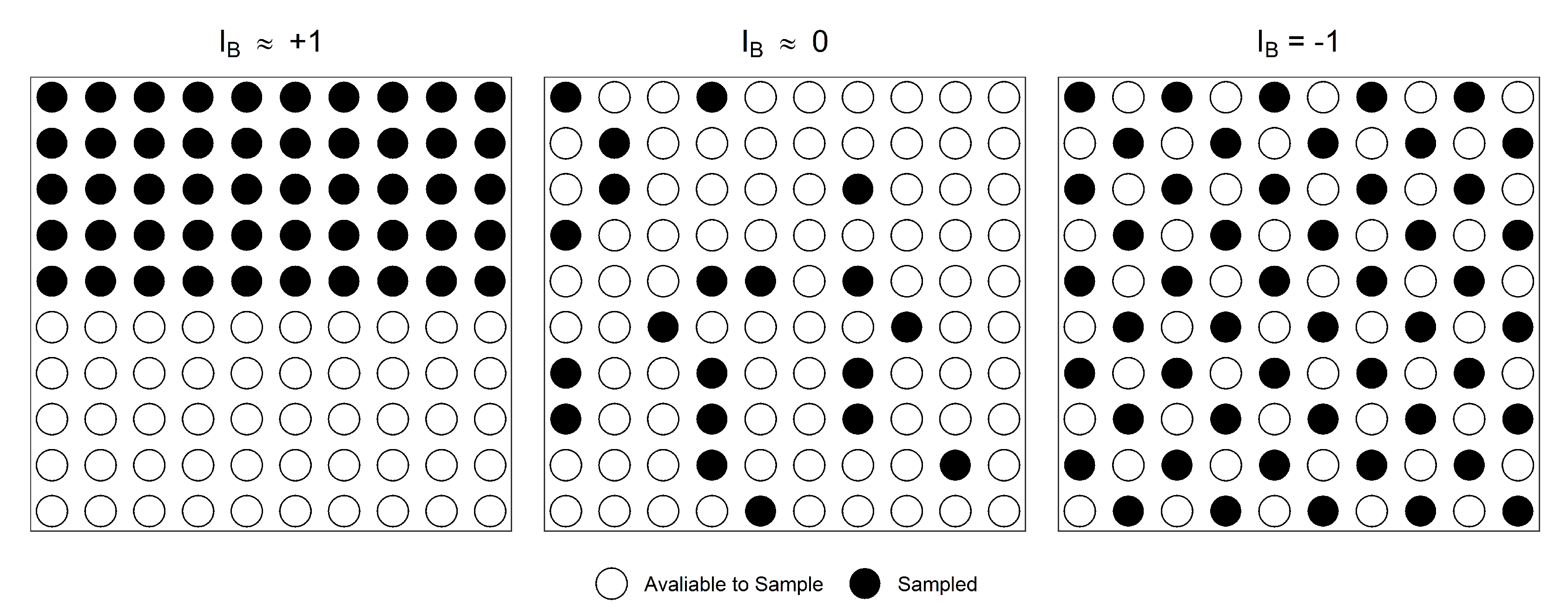
Similar to , is bounded: the lower bound (−1) indicates maximum balance and the upper bound (+1) indicates no balance; 0 corresponds to the spread of a random sample (Figure 1). To define , one has to account for the distance among population points and their inclusion probabilities (0 < ≤ 1) in order to identify neighbourhood relationships. Here, distances are computed based on remotely-sensed data. If i belonged to sample S, i would represent points in the population and, consequently, it would have neighbours according to a distance measure such as the Euclidean distance. Let and be the inferior and superior integers of , respectively, and let be the set of the nearest neighbours of i, where if . Then, can be specified as
For example, if = 6.9, this weighting scheme indicates that the 6 nearest neighbours of unit i have a weight of 1 while the 7th nearest neighbour has a weight of . If there are two or more th points at the same distance of i, is divided equally among them.
2.2. The T Index: How Reliable Are Accuracy Estimates Obtained from Non-Probability Samples?
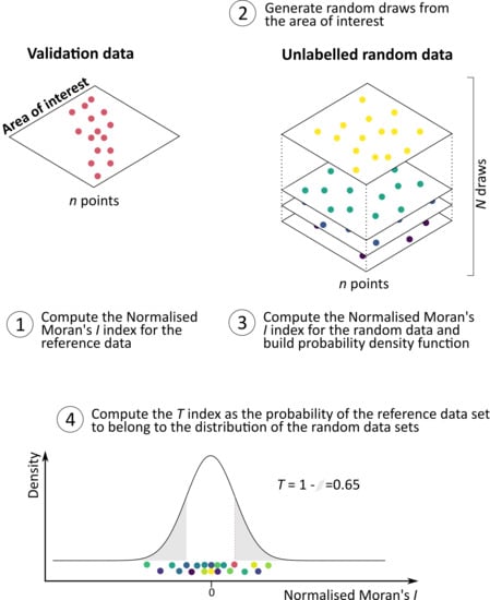
The T index evaluates if non-probability samples can yield reliable map accuracy estimates. Its computation is a four-step procedure to measure the strength of evidence that hold-out samples are in fact simple random samples (Figure 2).
Let us consider a hold-out data set (S) for which the sampling design is unknown. Its spread in the feature space can be measured by the normalised Moran’s I index (). The probability distribution of the normalised Moran’s I index for random samples of the same size as S () can be estimated by drawing random unlabelled samples from the population U and parametric or non-parametric approaches. On average, random samples take the value of zero but dispersion around the mean will depend largely on randomness and the size of S. Based on the empirical probability distribution of values for random samples, the T index is defined as the probability of a randomly-drawn data set to have the same spread in the feature space as the labelled set. This is expressed mathematically as follows,
where is the probability density function of values obtained from random unlabelled data. As integrates to one, T is bounded between zero and one. High values of T indicate that the labelled sample is very likely to be a random sample of the population and that the accuracy estimate of the cross-validation is a reliable approximation of the accuracy across the area of interest. Contrarily, values close to zero indicate that the labelled sample strongly violates the assumption of random sampling, and that the cross-validation results cannot be trusted, i.e., generalised to the map population. Therefore, the T index compares the value of the hold-out set to those of random unlabelled sets of the same size to indicate if the accuracy estimates can be trusted. Note that the procedure to construct the T index shares similarities with the bootstrap [16]. Unlike the bootstrap, the T index random draws samples (without replacement) from the population.
To maintain consistent nomenclature when describing the reliability of accuracy estimates obtained using non-probability samples, we propose to interpret the T index similar to p-values for significance testing. Here, the null hypothesis is that the hold-out set is a simple random sample of the map population. It follows that T values <0.05 indicate poor reliability: the corresponding accuracy estimates are unlikely to reflect map accuracy. T values ≥0.05 indicate substantial reliability: accuracy estimates are likely to be representative of map accuracy. This nomenclature provides a useful benchmark for the discussion and comparison of specific cases. Its relevance is demonstrated in the case study that follows.
3. Case Study
This case study illustrates the use and value of the T index in the context of crop mapping, an application where roadside data collection is common [17]. Crop types were identified based on time series of Harmonised Landsat Sentinel images and random forest classifiers. It was designed to empirically demonstrate that
- the normalised Moran’s I index correlates with the bias of accuracy estimates obtained from the reference data, and
- the T index indicates when cross-validated accuracy estimates can be trusted and generalised to the area of interest.
3.1. Data Sources
The study site is the state of Kansas, USA, for the 2017 growing season. The Cropland Data Layer (CDL) for 2017 was sourced from the United States Department of Agriculture National Agricultural Statistics Service and was considered as ground truth. A wall-to-wall reference map is a cost-effective approach to generate and compare different sampling strategies. The quality of our training and evaluation thus depends on the quality of the CDL. Evidence from published literature suggests that the quality of the CDL is sufficient to deliver consistent results, see, e.g., in [18,19]. Nonetheless, only the six dominant crop types (alfalfa, corn, wheat, fallow, sorghum and soybeans) were considered as the CDL is less accurate for marginal crop types [9]. In 2017, the overall accuracy of the map was 87% with class-wise biases ranging from 1% (wheat) and 3% (sorghum) to 4% (fallow) and 12% (alfalfa).
Harmonised Landsat Sentinel images (version 1.4) were collected from January 1 to December 31 2017 (15 tiles: 14SLG, 14SLH, 14SLJ, 14SMG, 14SMH, 14SMJ, 14SNG, 14SNH, 14SNJ, 14SPG, 14SPH, 14SPJ, 14SQG, 14SQH and 14SQJ [20]). On average, there were 103 images per tile and 32% of valid observations per image. Regular, gap-free time series were resampled to 10 days starting from day of year 60 to 330 using linear interpolation. The final data set consisted of 28 gap-free and regularly-spaced images with six spectral bands (blue, green, red, near infrared, short-wave infrared and red-edge).
3.2. Sampling and Classification
Three types of data sets were generated from the reference map: (1) 400 labelled sets covering a range of sample selection biases and from which training (n = 750) and hold-out sets were defined (n = 250); (2) 150 random unlabelled sets of the same size as the hold-out sets (n = 250), which were used to determine the distribution of for random data in the study area; and (3) a pseudo-population consisting of 10,000 randomly selected pixels, whose sole objective was to reduce computational cost associated with computing the .
Sample selection biases for the labelled data were introduced based on stratification layers. There were 16 stratification layers that partitioned the study area into up to 16 strata (Figure 3). For each stratification layer, a simple random sample was drawn within a single stratum that was itself selected at random. This process was repeated 25 times per stratification layer. By constraining sampling to a single stratum, the likelihood of capturing partial environmental and management gradients increases, with the net effect of reducing the spread of reference data in the feature space.
Random forest classifiers were trained for each labelled set. Random forests are a type of machine-learning classifier that is commonly used in remote sensing given their performance and easy parameterisation [21]. The number of trees was set to 500 and the number of variables to possibly split at in each node was the (rounded down) square root of the number variables.
The of every random unlabelled set was computed, and the corresponding probability distribution constructed using a non-parametric, kernel method. Similarly, the of hold-out sets was computed. Their corresponding T index was calculated using the probability distribution obtained for random unlabelled data. Note that, while all bands were used for classification, the Normalised Moran’s I Index was calculated based on the first five principal components of the feature space to further reduce computational complexity and memory requirements.
3.3. Statistical Analysis
First, was defined as the difference between estimates of overall accuracy obtained with hold-out data and those obtained with an independent, simple random sample (n = 250) extracted from the CDL. A positive bias indicates that the hold-out set overestimates overall accuracy, and vice versa. We also evaluated the relationship between the normalised Moran’s I index and bias using linear regression and computed the coefficient of determination (R) to quantify the proportion of the variability in bias explained by the .
Second, we assessed the ability of T to detect random samples for different threshold values. At each threshold value, we computed to overall accuracy (percentage correct), the sensitivity (proportion of actual positives that are correctly identified as such) and the specificity (proportion of actual negatives that are correctly identified as such).
4. Results and Discussion
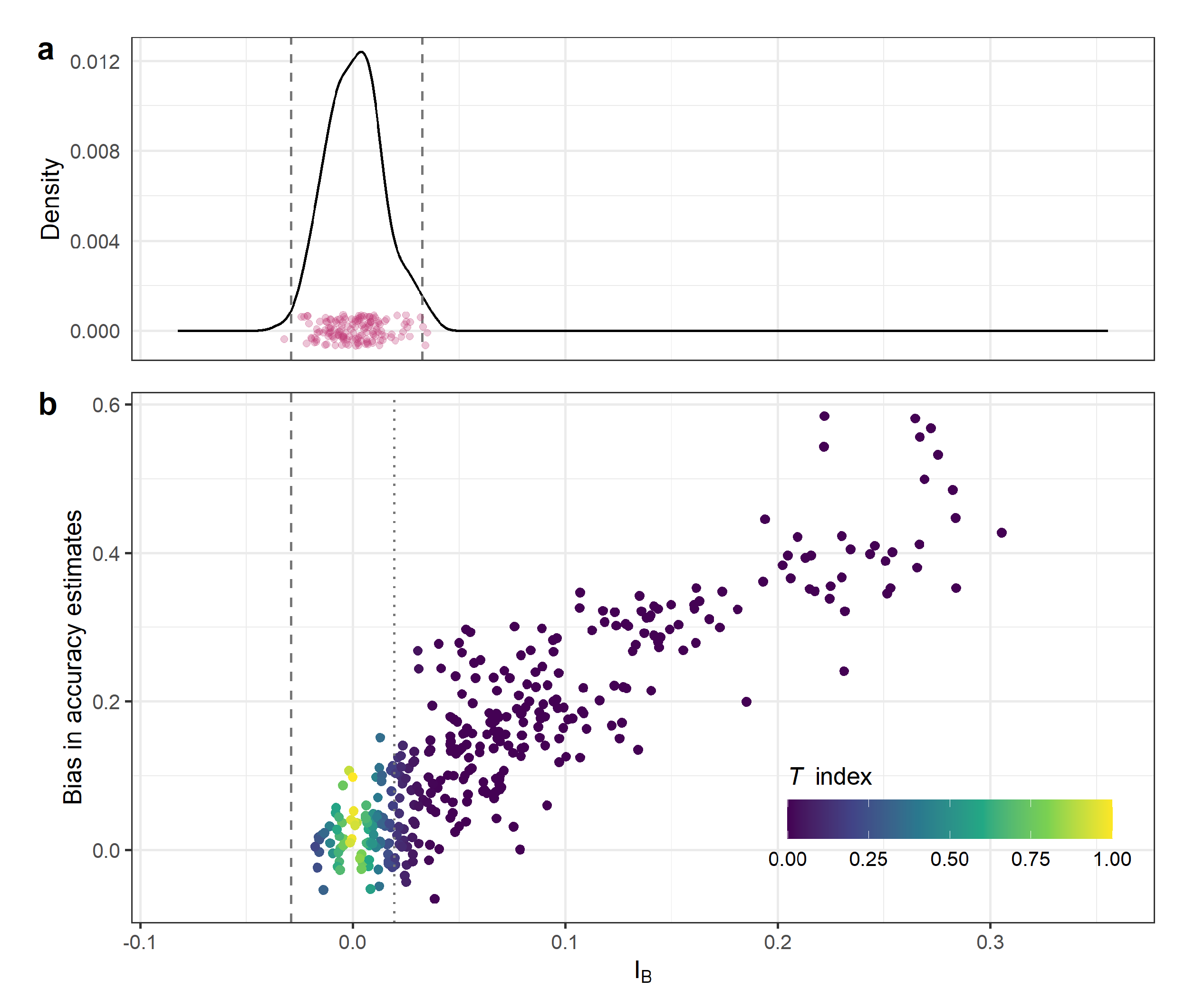
The successfully indicates bias in accuracy estimates obtained by non-probability samples. The stratification approach allowed us to generate values ranging from −0.08 to 0.36, which led to significant biases (up to 0.6; Figure 4). That is, accuracy estimates obtained from non-probability samples largely overestimated map accuracy. There was a significant positive linear relationship between and bias (). The closer to 0 the , the lower the bias. The larger the , the lower the bias. These findings are consistent with Fowler et al. [11] who reported significant correlations between and classification accuracy.
We also found that the T index accurately identified simple random samples among a set of samples with selection biases (Figure 5). Overall accuracy peaked at 0.90 or at a T value of 0.05, which seems to validate the proposed interpretation of T index. This T value also coincided well with the crossing of the sensitivity and specificity curves. Therefore, the T index can indicate when accuracy estimates obtained from non-probability samples are representative of map accuracy.
The T index leverages one of the strengths of remote-sensing data about the complete spatial population are available—to indicate the extent to which users can trust cross-validated accuracy estimates. That is, the T index quickly informs practitioners and map users if cross-validation does not provide reliable estimates of map accuracy. As it does not require data other than the remotely-sensed observations used for classification, it can always be computed. The main drawback of using the T index is its computational cost. It requires computing of the normalised Moran’s I index of multiple random unlabelled samples, which involves computing distances between all points in the population. There are at least two approaches to reduce computational cost: First, the complexity of the problem can be reduced. For instance, we reduced the dimensionality of the feature space using a principal component analysis and reduced the size of the population by selecting a subset of the map population. Despite these simplifications, our results showed that the T index was still indicative of the representativeness of validation sets. Second, the implementation of the should rely on high-performance data analytics. Our code was run on a high-performance computing system and explicitly stores large matrices in files, not in computer memory (https://github.com/waldnerf/t-index). Together, these approaches allow to derive the T index for big Earth Observation data. We recommend that studies that assess accuracy by cross-validation or with non-probability samples start systematically reporting the corresponding T index. Uptake of the T index by the remote-sensing community would directly answer the call by Stehman and Foody [1] to improve documentation and enhance transparency of accuracy assessment methods. As such, it fosters trust in accuracy estimates when reference data have not been collected following probability sampling.
As a first step in this direction, this letter focuses on the most simple case: hold-out validation. This letter also signals future considerations such as generalising the T index to other types of cross-validation designs, other accuracy metrics or other classification/validation settings (object-based approaches). There is also scope for integrating the T index with importance-weighted cross-validation [22]. Under sample selection bias, importance-weighted cross-validation can provide, in principle, unbiased accuracy estimates by weighting validation data by a factor that matches their observation probability in the population. However, the performance of this technique is only as good as the estimates of importance, which is not without challenges [23,24]. While there is little doubt that the use of importance-weighted cross-validation should be promoted, the remote-sensing community would benefit from guidelines on when it must be used; this paper could inform such guidelines. For instance, a rule of thumb could mandate importance-weighted cross-validation for T values < 0.05. Its relevance remains to be tested empirically.
5. Conclusions
When independent probability data are lacking, maps are often “validated” by cross-validation of non-probability data. While it is well known that the accuracy estimates obtained in this fashion are not representative of map accuracy, there is currently no method to evaluate how much these differ from one another. The T index presented in this letter provides a quantitative response to this question. It is directly interpretable as the probability of a validation set to be a simple random sample of the map population, an assumption that must be verified for cross-validation to provide representative estimates of map accuracy with hold-out cross-validation. As a probability, the T index is bounded between zero and one and guidelines for consistent interpretation are proposed based on the significance testing, where T values <0.05 indicate unreliable accuracy estimates. Systematic reporting of the T index alongside accuracy metrics is recommended to provide users with objective, quantitative information about the reliability of accuracy estimates obtained from non-probability samples so that they can decide whether the map is fit for their purpose and gauge how its accuracy impacts their application. Therefore, its uptake by the remote-sensing community will promote trust in accuracy assessment and transparency, which is particularly desirable when dealing with data sets that deviate from gold standards.
Funding
The author acknowledges the support of the Digiscape Future Science Platform, funded by the CSIRO.
Acknowledgments
The author would like to thank Giles Foody, Rob Garrard, and the anonymous reviewers for their insightful comments on this manuscript. We also thank Diego Giuliani and Yves Tillé for sharing their R implementation of the normalised Moran’s I index.
Conflicts of Interest
The author declares no conflicts of interest.
Code Availability
An implementation of the T index is provided at https://github.com/waldnerf/t-index.
References
- Stehman, S.V.; Foody, G.M. Key issues in rigorous accuracy assessment of land cover products. Remote Sens. Environ. 2019, 231, 111199. [Google Scholar] [CrossRef]
- Stehman, S.V. Basic probability sampling designs for thematic map accuracy assessment. Int. J. Remote Sens. 1999, 20, 2423–2441. [Google Scholar] [CrossRef]
- Liu, C.; Frazier, P.; Kumar, L. Comparative assessment of the measures of thematic classification accuracy. Remote Sens. Environ. 2007, 107, 606–616. [Google Scholar] [CrossRef]
- Stehman, S.V. Sampling designs for accuracy assessment of land cover. Int. J. Remote Sens. 2009, 30, 5243–5272. [Google Scholar] [CrossRef]
- Pontius, R.G., Jr.; Millones, M. Death to Kappa: Birth of quantity disagreement and allocation disagreement for accuracy assessment. Int. J. Remote Sens. 2011, 32, 4407–4429. [Google Scholar] [CrossRef]
- Olofsson, P.; Foody, G.M.; Herold, M.; Stehman, S.V.; Woodcock, C.E.; Wulder, M.A. Good practices for estimating area and assessing accuracy of land change. Remote Sens. Environ. 2014, 148, 42–57. [Google Scholar] [CrossRef]
- Zhu, Z.; Gallant, A.L.; Woodcock, C.E.; Pengra, B.; Olofsson, P.; Loveland, T.R.; Jin, S.; Dahal, D.; Yang, L.; Auch, R.F. Optimizing selection of training and auxiliary data for operational land cover classification for the LCMAP initiative. ISPRS J. Photogramm. Remote Sens. 2016, 122, 206–221. [Google Scholar] [CrossRef] [Green Version]
- Heydari, S.S.; Mountrakis, G. Effect of classifier selection, reference sample size, reference class distribution and scene heterogeneity in per-pixel classification accuracy using 26 Landsat sites. Remote Sens. Environ. 2018, 204, 648–658. [Google Scholar] [CrossRef]
- Waldner, F.; Chen, Y.; Lawes, R.; Hochman, Z. Needle in a haystack: Mapping rare and infrequent crops using satellite imagery and data balancing methods. Remote Sens. Environ. 2019, 233, 111375. [Google Scholar] [CrossRef]
- Foody, G.M.; Mathur, A. Toward intelligent training of supervised image classifications: Directing training data acquisition for SVM classification. Remote Sens. Environ. 2004, 93, 107–117. [Google Scholar] [CrossRef]
- Fowler, J.; Waldner, F.; Hochman, Z. All pixels are useful, but some are more useful: Efficient in situ data collection for crop-type mapping using sequential exploration methods. Int. J. Appl. Earth Obs. Geoinf. 2020, 91, 102114. [Google Scholar] [CrossRef]
- Morales-Barquero, L.; Lyons, M.B.; Phinn, S.R.; Roelfsema, C.M. Trends in remote sensing accuracy assessment approaches in the context of natural resources. Remote Sens. 2019, 11, 2305. [Google Scholar] [CrossRef] [Green Version]
- Lyons, M.B.; Keith, D.A.; Phinn, S.R.; Mason, T.J.; Elith, J. A comparison of resampling methods for remote sensing classification and accuracy assessment. Remote Sens. Environ. 2018, 208, 145–153. [Google Scholar] [CrossRef]
- Tillé, Y.; Dickson, M.M.; Espa, G.; Giuliani, D. Measuring the spatial balance of a sample: A new measure based on Moran’s I index. Spat. Stat. 2018, 23, 182–192. [Google Scholar] [CrossRef] [Green Version]
- Moran, P.A. Notes on continuous stochastic phenomena. Biometrika 1950, 37, 17–23. [Google Scholar] [CrossRef]
- Efron, B. Bootstrap methods: Another look at the jackknife. In Breakthroughs in Statistics; Springer: Berlin, Germany, 1992; pp. 569–593. [Google Scholar]
- Waldner, F.; Bellemans, N.; Hochman, Z.; Newby, T.; de Abelleyra, D.; Verón, S.R.; Bartalev, S.; Lavreniuk, M.; Kussul, N.; Le Maire, G.; et al. Roadside collection of training data for cropland mapping is viable when environmental and management gradients are surveyed. Int. J. Appl. Earth Obs. Geoinf. 2019, 80, 82–93. [Google Scholar] [CrossRef]
- Sun, W.; Liang, S.; Xu, G.; Fang, H.; Dickinson, R. Mapping plant functional types from MODIS data using multisource evidential reasoning. Remote Sens. Environ. 2008, 112, 1010–1024. [Google Scholar] [CrossRef]
- Whelen, T.; Siqueira, P. Use of time-series L-band UAVSAR data for the classification of agricultural fields in the San Joaquin Valley. Remote Sens. Environ. 2017, 193, 216–224. [Google Scholar] [CrossRef]
- Claverie, M.; Ju, J.; Masek, J.; Dungan, J.; Vermote, E.; Roger, J.; Skakun, S.; Justice, C. The Harmonized Landsat and Sentinel-2 surface reflectance data set. Remote Sens. Environ. 2018, 219, 145–161. [Google Scholar] [CrossRef]
- Breiman, L. Random forests. Mach. Learn. 2001, 45, 5–32. [Google Scholar] [CrossRef] [Green Version]
- Sugiyama, M.; Krauledat, M.; Muller, K.R. Covariate shift adaptation by importance weighted cross validation. J. Mach. Learn. Res. 2007, 8, 985–1005. [Google Scholar]
- Kouw, W.; Loog, M. Effects of sampling skewness of the importance-weighted risk estimator on model selection. In Proceedings of the 24th International Conference on Pattern Recognition (ICPR), Beijing, China, 20–24 August 2018; pp. 1468–1473. [Google Scholar]
- Kouw, W.M.; Krijthe, J.H.; Loog, M. Robust importance-weighted cross-validation under sample selection bias. In Proceedings of the IEEE 29th International Workshop on Machine Learning for Signal Processing (MLSP), Espoo, Finland, 21–24 September 2019; pp. 1–6. [Google Scholar]
Figure 1.
The Normalised Moran’s I Index () takes the value of +1 for clustered samples (left), 0 for random samples (centre) and −1 for spatially-balanced samples (right).
Figure 1.
The Normalised Moran’s I Index () takes the value of +1 for clustered samples (left), 0 for random samples (centre) and −1 for spatially-balanced samples (right).

Figure 2.
Procedure to construct the T index: (1) calculate the Normalised Moran’s I Index of the labelled hold-out set, (2) generate random unlabelled samples from the map population, (3) calculate the Normalised Moran’s I Index of all random unlabelled samples and (4) compute the probability of the labelled set to belong to the empirical distribution of random unlabelled samples.

Figure 3.
Area of interest in Kansas and the 16 stratification layers. The stratification layers were used to introduce sample selection biases in reference data. Colours represent different strata. Grey areas were not considered.
Figure 3.
Area of interest in Kansas and the 16 stratification layers. The stratification layers were used to introduce sample selection biases in reference data. Colours represent different strata. Grey areas were not considered.

Figure 4.
Relationship between Normalised Moran’s I Index () and map accuracy. (a) Empirical distribution of values for random unlabelled data sets. (b) Relationship between the of the labelled sets, their bias and corresponding T index. There is a strong linear relationship between and bias (; ). The dashed line indicates values for which the T index is 0.05.

Figure 5.
Ability of the T index to accurately identify representative (random) hold-out sets. Results validate the proposed nomenclature to interpret the T index.
Figure 5.
Ability of the T index to accurately identify representative (random) hold-out sets. Results validate the proposed nomenclature to interpret the T index.

© 2020 by the author. Licensee MDPI, Basel, Switzerland. This article is an open access article distributed under the terms and conditions of the Creative Commons Attribution (CC BY) license (http://creativecommons.org/licenses/by/4.0/).
Share and Cite
MDPI and ACS Style
Waldner, F. The T Index: Measuring the Reliability of Accuracy Estimates Obtained from Non-Probability Samples. Remote Sens. 2020, 12, 2483. https://0-doi-org.brum.beds.ac.uk/10.3390/rs12152483
AMA Style
Waldner F. The T Index: Measuring the Reliability of Accuracy Estimates Obtained from Non-Probability Samples. Remote Sensing. 2020; 12(15):2483. https://0-doi-org.brum.beds.ac.uk/10.3390/rs12152483
Chicago/Turabian StyleWaldner, François. 2020. "The T Index: Measuring the Reliability of Accuracy Estimates Obtained from Non-Probability Samples" Remote Sensing 12, no. 15: 2483. https://0-doi-org.brum.beds.ac.uk/10.3390/rs12152483
Note that from the first issue of 2016, this journal uses article numbers instead of page numbers. See further details here.