Fully Convolutional Neural Network for Rapid Flood Segmentation in Synthetic Aperture Radar Imagery


1
United Nations Institute for Training and Research’s (UNITAR) Operational Satellite Applications Programme (UNOSAT), CERN, 1211 Meyrin, Switzerland
2
United Nations Global Pulse, New York, NY 10017, USA
3
Institute for Data Science, Durham University, Durham DH1 3LE, UK
*
Author to whom correspondence should be addressed.
Remote Sens. 2020, 12(16), 2532; https://0-doi-org.brum.beds.ac.uk/10.3390/rs12162532
Submission received: 1 June 2020
/
Revised: 29 July 2020
/
Accepted: 30 July 2020
/
Published: 6 August 2020
(This article belongs to the Special Issue Machine and Deep Learning for Earth Observation Data Analysis)
Abstract
:Rapid response to natural hazards, such as floods, is essential to mitigate loss of life and the reduction of suffering. For emergency response teams, access to timely and accurate data is essential. Satellite imagery offers a rich source of information which can be analysed to help determine regions affected by a disaster. Much remote sensing flood analysis is semi-automated, with time consuming manual components requiring hours to complete. In this study, we present a fully automated approach to the rapid flood mapping currently carried out by many non-governmental, national and international organisations. We design a Convolutional Neural Network (CNN) based method which isolates the flooded pixels in freely available Copernicus Sentinel-1 Synthetic Aperture Radar (SAR) imagery, requiring no optical bands and minimal pre-processing. We test a variety of CNN architectures and train our models on flood masks generated using a combination of classical semi-automated techniques and extensive manual cleaning and visual inspection. Our methodology reduces the time required to develop a flood map by 80%, while achieving strong performance over a wide range of locations and environmental conditions. Given the open-source data and the minimal image cleaning required, this methodology can also be integrated into end-to-end pipelines for more timely and continuous flood monitoring.

1. Introduction
The efficiency and timeliness of emergency responses to natural disasters has significant implications for the life-saving capacities of relief efforts. Access to accurate information is crucial to these missions in determining resource allocation, personnel deployment and rescue operations. Despite the critical need, collecting such information during a crisis can be extremely challenging.
Floods are the most frequent natural disaster and can cause major societal and economic disruption longside significant loss of human life [1,2]. Flooding is usually caused by rivers or streams overflowing, excessive rain, or ice melting rapidly in mountainous areas. Alternatively, coastal floods can be due to heavy sustained storms or tsunamis causing the sea to surge inland. Once an event occurs, a timely and accurate assessment, followed by a rapid response, is crucial. In carrying out this response, non-governmental, national and international organizations are usually at the forefront of operations providing humanitarian support.
Remote sensing techniques have been crucial in providing information to response teams in such situations [3]. Indeed, satellite images have proved highly useful for collecting timely and relevant data and in generating effective damage information and impact maps of flooded regions [4,5]. Currently, much of the flood analysis is manual or semi-automated, and carried out by experts from a range of organizations. One example of such an institution is the United Nations Institute for Training and Research—Operational Satellite Applications Programme (UNITAR-UNOSAT), who provide a ‘Rapid Mapping’ service [6], and against whose methodology we base our comparison. In general, in order to respond to quickly developing situations, rapid mapping methodologies serve as an instrumental component in emergency response and disaster relief.
Traditionally, a common way to approach water and flood detection is to use imagery collected from passive sensors, such as optical imagery, using techniques such as the Normalized Difference Water Index (NDWI) and other water indices [7,8,9,10]. In such cases, numerous methods have been developed for combining different frequency bands in order to produce signatures particularly sensitive to the detection of water bodies. Once an index has been calculated, water and flood detection can be carried out through the use of thresholds which can either be set globally over the entire region in question, or more locally. While such detection algorithms using optical imagery, and other multispectral imagery derived from passive sensors, have shown great promise, the use of such imagery is often subject to lack of cloud cover and the presence of daylight. These requirements restrict their use to a limited time interval and to certain weather conditions thus making them less suitable for rapid response in disaster situations.
For this reason, one of the most commonly used forms of satellite data used for flood water detection is Synthetic Aperture Radar (SAR) imagery [11]. SAR images can be taken regardless of cloud cover and time of day since they use active sensors and specific frequency ranges. Although SAR images generally have a lower resolution in comparison to their high-resolution optical counterparts, high-resolution imagery (to the level of 0.3–0.5 m) is not generally required for flood disaster mapping, and SAR imagery can be taken at an acceptable resolution. Due to their popularity, many SAR satellite collaborations, such as COSMO-SkyMed (CSK) [12], TerraSAR-X (TSX) [13], and Sentinel-1 operated by the European Space Agency (ESA) now exist, making for regular and timely image capture.
The detection of water bodies in SAR imagery is largely reliant on the distinctiveness of its backscatter signature. Water generally appears as a smooth surface with a well defined intensity of backscatter that can be seen in the SAR image; however, depending on environmental conditions such as landscape topography and shadows, a universal threshold for water backscatter intensity does not exist. Furthermore, there are also particular exceptions that require more careful consideration rather than just threshold setting. In the case of urban areas, for instance, the backscattered signal can be significantly affected by the presence of buildings that exhibit double-bounce scattering, although several techniques have been designed to address this [14,15,16,17,18,19]. Indeed, similar considerations may need to be made for numerous other cases such as water otherwise masked by vegetation [20]. In this study, we will focus on general water/flood detection by developing a method which generalizes across different environments, some of which contain urban regions, although we do not focus specifically on addressing such areas.
Since flooding can occur in a variety of different environmental settings, the generalizability of many existing methods is highly limited, often requiring the careful intervention of analysts to update parameters and fine-tune results. Such tuning severely limits the speed with which accurate maps can be produced and released for use by disaster response teams. Moreover, many of these methods require the combination of data from a variety of sources, as well as extensive cleaning and processing of imagery before they can be fully utilized. While there have been some successes in near real time (NRT) mapping [21,22,23,24], such methods generally still succumb to the generalizability shortfalls highlighted above. However, Twele et al. [25] have presented an NRT approach requiring no human intervention and significantly reducing processing time, by using fuzzy logic techniques, which have since been built on [26,27], to remove the need for additional input data.
Machine learning techniques have been shown to offer increasingly generalizable solutions to a range of problems previously requiring a significant amount of classical image processing [28,29], and have been applied to a wide variety of fields while gaining prevalence in applications to satellite imagery [3,30,31,32]. Specifically, machine learning techniques are now being developed for water detection, with several focusing on flood mapping as we discuss below.
With the increased rapid deployment of satellites providing low-cost optical imagery, such as CubeSats, several applications of machine learning methods to automate water/flood detection in optical and multispectral imagery have been developed [33,34,35,36,37,38,39]. However, since imagery from passive sensors is limited by the conditions mentioned above, such as cloud cover, they are therefore often not appropriate for flood response. Interestingly, work such as that by Benoudjit and Guida [40] take a hybrid approach by using a linear model optimized with stochastic gradient descent to infer flooded pixels in SAR imagery with promising results and a dramatic reduction in the time required to infer on an image. However, as the authors point out, training data is generated per-location from calculation of the NDWI which therefore still requires the use of imagery containing additional frequency bands.
There have been several studies applying Artificial Intelligence (AI) techniques requiring only SAR imagery for water/flood identification. For this, a variety of methods have been tested including unsupervised learning techniques such as self-organizing Kohonen’s maps [41,42], Gaussian Mixture Models [43], and support vector machines [44] for general flood mapping. One of the most commonly used techniques in machine learning for pixel-based segmentation is that of Convolutional Neural Networks (CNNs). Several studies have been shown to make use of these networks for multiclassification tasks (including a water class), for example, in complex ecosystem mapping [45], urban scene and growth mapping [46], and crop identification [47]. In such cases, water detection has not been the central aim of the outputs, and so such methodologies have not been optimised for its identification. Moreover, flooding causes the presence of water bodies on both large and small scales and so work lacking this focus is not sufficient by itself to provide evidence that CNN methods can be widely applied to flood events.
Focusing on large water bodies and flood events, various CNN approaches have been proposed for different scenarios. In the specific case of urban flood mapping, for example, Li et al. [48] select a specific location and use multi-temporal SAR imagery to develop an active self-learning approach to CNN training, showing improved performance against a naively trained classifier. In addition, Zhang et al. [49] compare several CNN based approaches for the identification of water and shadows. However, their focus on a limited range of locations and reliance on flood maps created by hand, rather than also incorporating classical methods, may be overly simplified. Most similar to the work presented here is that of Kang et al. [50] who use a CNN specifically for flood detection in SAR imagery captured in China. The authors show that using CNNs for flood mapping may be a viable option—achieving promising metrics and performance. We seek to build on this work in demonstrating the generalizaility of a CNN approach by training and testing our models on a dataset reaching over multiple countries and regions including many of those which are significantly disaster prone. Moreover, the authors of [50] highlight the desire to test the usefulness of transfer learning approaches in future work, which we shall also study.
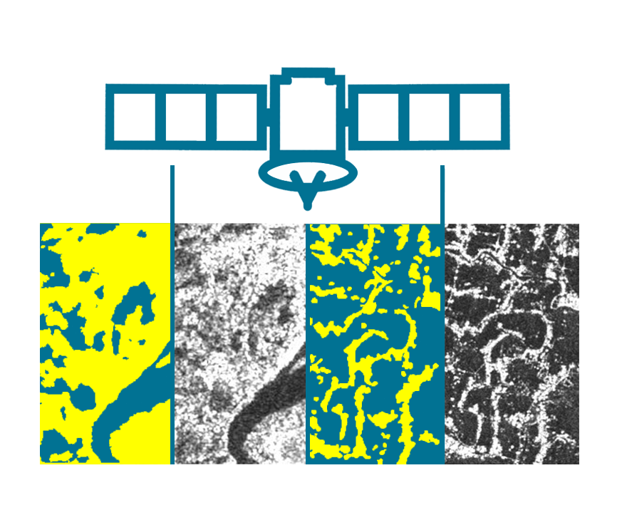
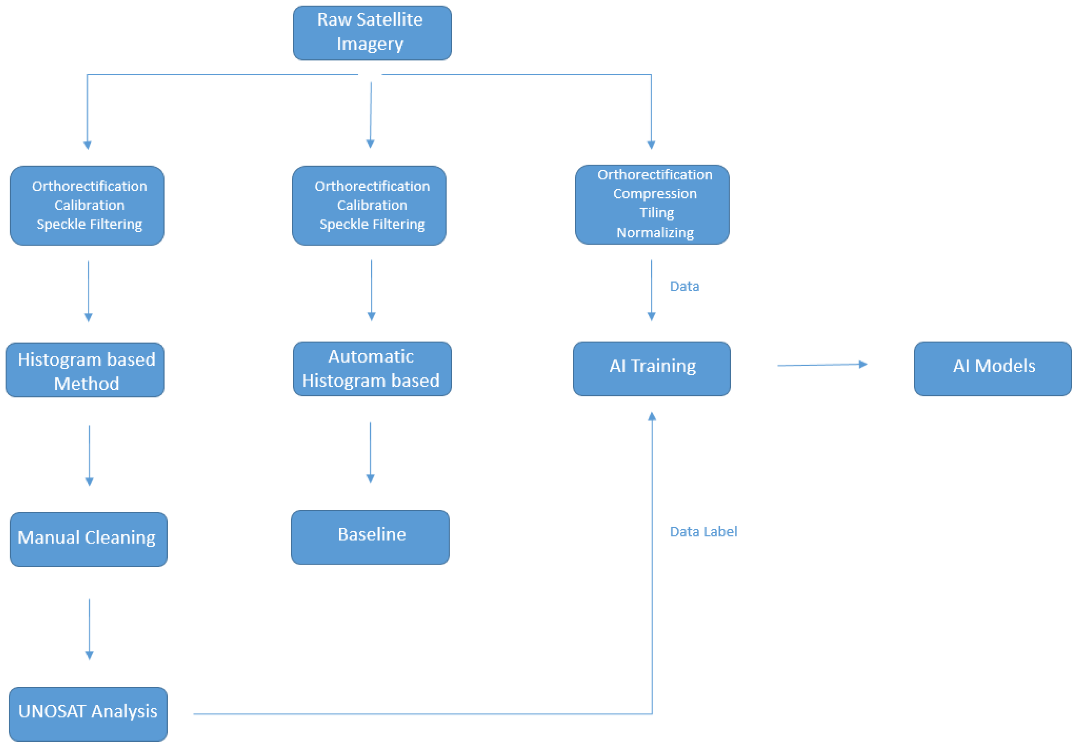
In this paper we present a fully automated machine learning based solution for rapid mapping, significantly decreasing the time required to produce a flood map, while achieving a high level of precision in comparison to existing classical methodologies involving significant manual intervention. The model is trained on a fully open-source dataset presented here, which we compile from imagery frequently used in disaster response situations. Furthermore, this dataset contains analysis performed during rapid mapping response scenarios and so presents an ideal test bed for trialing rapid mapping automation techniques. We believe this to be the largest and most diverse SAR dataset that machine learning based flood mapping models have been developed for and tested against. The methodology employed for the creation of the labels used for model training consists of a classical histogram based method followed by extensive manual cleaning and visual inspection as explain in Section 2.2. In addition, we design a simple linear baseline model against which to compare our more complex machine learning approaches as explained in Section 2.4. Our methodology does not require any additional pre-processing or input data, apart from orthorectification using a digital elevation model (DEM), as well as computationally inexpensive tiling, compression and normalisation as explain in Section 2.3, thereby making it a strong contender for fully automated pipelines. Moreover, this method only requires the use of open-source Sentinel-1 SAR imagery and can, if required, be fine-tuned to the analysis area by adding human-in-the-loop (HITL) network adaptation into the mapping pipeline [51]. While this fine-tuning is not necessarily required in our circumstances, we discuss how it can be naturally incorporated into the pipeline with minimal extra time cost and may aid in alleviating difficulties experienced in classical SAR analysis. Since flooding generally occurs adjacent to existing bodies of water, flood detection usually includes the detection of all water bodies, including those permanent to the scene. Since permanent water bodies are usually already mapped and can be subtracted out to measure flood growth, we go beyond other studies in explicitly examining the performance of our methodology in both general water detection, as well as just flood detection. We finish this paper by presenting a cost-benefit analysis, comparing our methodology to currently employed tools and highlight the applicability of this technique to rapid mapping for disaster response, including setting out a potential work flow which incorporates model validation and improvement. This work has been carried out in collaboration with several United Nations (UN) entities, including UNOSAT, upon whose workflow we base our comparison. For further information, please visit the GitHub project (https://github.com/UNITAR-UNOSAT/UNOSAT-AI-Based-Rapid-Mapping-Service). For clarity, a general overview of the comparisons made in this paper is depicted in Figure 1.
2. Materials and Methods
2.1. Dataset
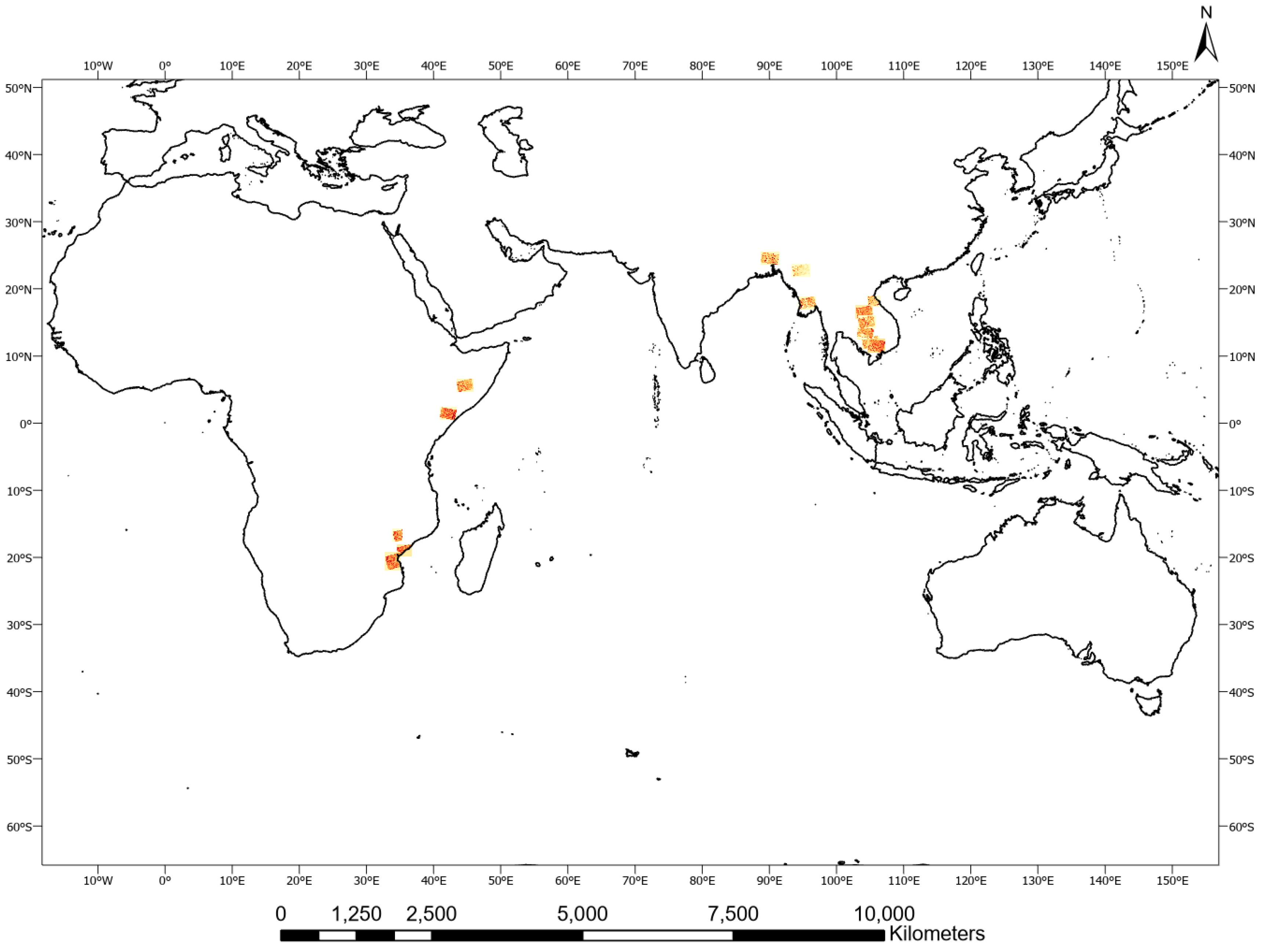
The UNOSAT Flood Dataset [52], has been created for this study using Copernicus Sentinel-1 satellite imagery acquired in Interferometric Wide Swath (IW) and provided as Level-1 Ground Range Detected (GRD) products at a resolution of 10 m × 10 m with corresponding flood vectors stored in shapefile format (see Figure 2). Each image was downloaded from the Copernicus Open Access Hub [53] in order to work on free and open-source data thereby facilitating the deployment of our methodology more broadly (see Table 1 and Table A1 for more details on the dataset).
The dataset consists of the VV polarization of the SAR imagery with their corresponding flood extent boundaries. These boundaries were taken from preexisting UNOSAT analyses conducted over a five year period generated using the commonly used histogram based method (also known as the threshold method) and followed by extensive manual cleaning and visual inspection for noise reduction and precision validation (see Section 2.2). Flood maps generated using this method were used as labels for training our machine learning models. In addition, we experimented with applying a variety of pre and post-processing techniques to the SAR data and assessed its impact on model performance (see Section 2.3). It should be noted that we make no assessment of the thematic accuracy of the “labels" created using the techniques mentioned in Section 2.2 and used here for model training and inference. The potential for thematic accuracy assessments and field-level feedback for model improvement are discussed in Section 4.5.
2.2. Histogram Based Method and Label Generation
The aim of flood detection analysis using satellite imagery is to extract water signatures and convert them to cleaned vector data. In both radar and optical imagery bands, there is a contrast between water and non-water pixels. In the former case, water pixels generally appear significantly darker than non-water pixels after the usual processing applied by the imagery provider. Using a histogram based method is common practice when identifying water pixels in SAR imagery for disaster mapping [21,54,55,56,57].
When using this method, a sample of pixel values is manually taken from the visible flood extent in the radar image to estimate the range of pixel values that represent water. All pixels that are within that pixel value range are then selected by the algorithm. Often, experiments will be conducted with multiple thresholds to determine which value provides the most accurate output based largely on visual inspection and comparison with pre-flood information (i.e., data on the location of rivers and other existing water bodies). A standard end-to-end pipeline for rapid flood analysis, following the work of [21,54,55,56,57], is described below:
- A raw satellite image is imported, pre-processed and calibrated through radiometric correction. After this, the image undergoes speckle filtering followed by orthorectification using a DEM.
- Multiple thresholds are then determined to separate water and land through manual pixel sampling and applied to the image. Running the analysis for each threshold value can take from five to ten minutes each time using standard GIS mapping software. This extraction may either underestimate or overestimate the flood and therefore expert knowledge provided by an analyst is crucial in determining the best threshold value.
- The new raster images will have two values: the ‘1’ values representing the threshold extraction, and the ‘0’ values representing the corresponding pixels that were above the threshold. A new raster image is created for each chosen threshold.
- Since the selected extraction is an approximation, it requires filtering to smooth the edges of the water signature. Majority Filtering [58] is applied to reducing noise and fill in ‘holes’ in the water extent.
- A Focal Statistics method [59] is then applied to help further smooth and remove additional noise.
- The best raster according to the analyst is converted to a vector.
- The flood vector is further cleaned by manual inspection to: remove Zero Grid values to save only the flooded area; remove the imagery border; further reduce noise; fill in any remaining holes and remove any other obvious non-water elements.
- The river and other water resources that were present in the pre-flood analysis are then filtered out and excluded from the flooded area.
As can be seen, this methodology involves much expert manual intervention and cleaning to produce a flood map. Limitations of this methodology are possible false positive/negative values in areas of radar overlays, foreshortening, and shadows in hilly and mountainous areas which may affect algorithmic performance. Dense urban areas and smooth areas like roads and dry sand can further affect performance. Furthermore, ‘holes’ in the dataset are pixels or groups of pixels formed where a water signature was not detected. This may occur due to different signatures in the imagery such as hill shadow in a mountainous area, waves and boats in the water, and vegetation or structures like bridges that may cause false water signatures in the extraction.
The generation of labeled data denoting water extent can depend on a variety of external factors. Human errors must be taken into consideration since, even though the analyst follows a strict workflow, the flood boundaries are chosen based on human experience. The quality of the flood map is also influenced by time restrictions since rapid assessment flood maps must frequently be delivered in a few days. Moreover, sending feedback from the flooded regions to the map provider may not always be possible during a humanitarian emergency.
For completeness, potential human biases were estimated by conducting four independent analyses, each following the procedure described above, on a random subset of the images comprising our dataset. In each case, the difference between the archived and a new analysis of the same image was calculated. The analyses were found to differ by 5% on average in both classes, which serves as a lower bound on the variability of the labels used. In addition, in an attempt to minimize the human error, the entire dataset was reviewed through visual inspection by two different geospatial analysts with necessary modifications made to increase consistency. The flood vectors generated with this method were used as labels for our machine learning approaches. The analyses can be downloaded from the UNOSAT Flood Portal [60], and the UNOSAT page on the Humanitarian Data Exchange [61].
2.3. Data Processing for Machine Learning
To assess their impact on model performance, we experimented with a variety of data processing techniques. First, a terrain correction was applied using the orbit file as is standard procedure when delivering the final output. After testing various image pre-processing techniques prior to model training, including speckle filtering and calibration, we observed best performance when such processing was minimised to just orthorectification and compression to 8-bit. We perform this latter step since we found it to make image storage and manipulation more memory efficient without hindering overall performance. By reducing the necessary pre-processing, the time required to produce a map is also reduced. Concerning the labels, a binary mask was generated from the shapefiles where the flood pixels were labeled as one and the background as zero. These masks were clipped with the corresponding satellite image.
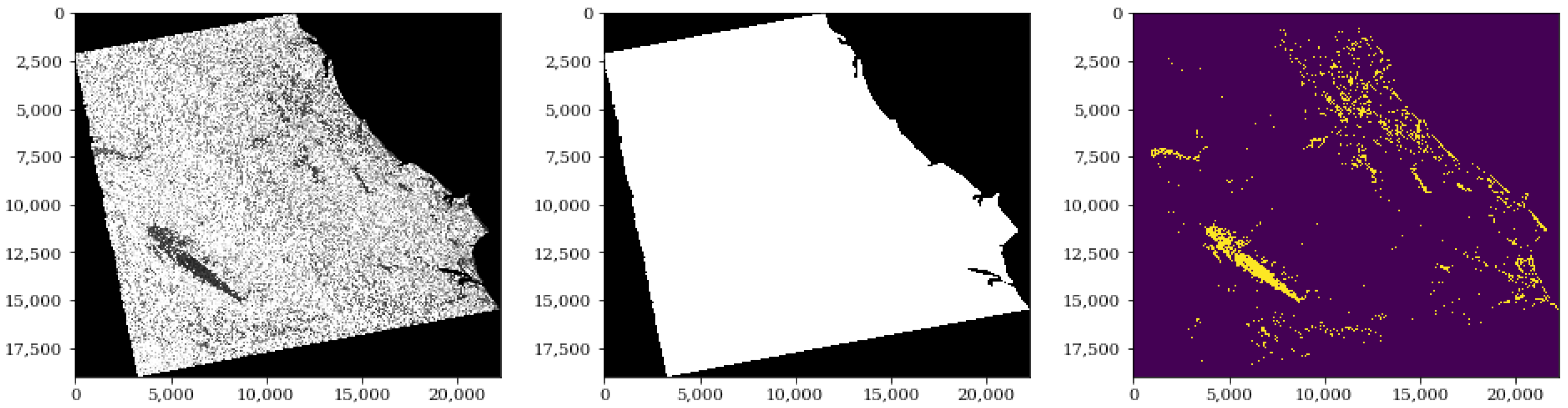
The image comes with a black frame around it that can have different default values such as nan, -inf, and others. The sea areas can also be characterized by outliers from shadows due to waves and high values due to ships. For the purposes of the labels, the sea was originally assigned as water up to a certain distance from the coastline which varied each time. Therefore, for consistency, the sea and the black frame around the image were masked out using the image extent and a global coastal shapefile, as shown in Figure 3. These regions were not included in the dataset. Moreover, to avoid confusing the network, existing water bodies, such as rivers, were added back to the labeled data in order for the network to learn to detect all water pixels as opposed to only newly flooded regions.
Feeding a neural network with the entire satellite image is not computationally feasible, due to their large memory footprint. Therefore, we tiled the images, and their corresponding labels, prior to training. Different tile sizes were tested, with best performance being observed with tiles sized 256 × 256 pixels. For clarity, throughout this paper we refer to ‘images’ as the raw SAR imagery obtained from the image provider and ‘tiles’ as the output from tiling the images.
The dataset was split into training, validation and testing sets following a ratio 80:10:10. The training dataset is used to train the candidate algorithms, the validation dataset is used to tune the hyperparameters (e.g., the architecture, batch size etc.), and the test dataset is used to obtain the performance characteristics on tiles completely unseen by the model. The test set is independent of the training dataset, but it likely follows the same probability distribution as the training dataset since tiles in this set come from the same original image as tiles in the training and validation sets. In order to test performance more rigorously, we also present results derived from inference on tiles from a completely unseen image and location (see Section 3.2). The UNOSAT Flood Dataset and its tiles are shown in Table 1.
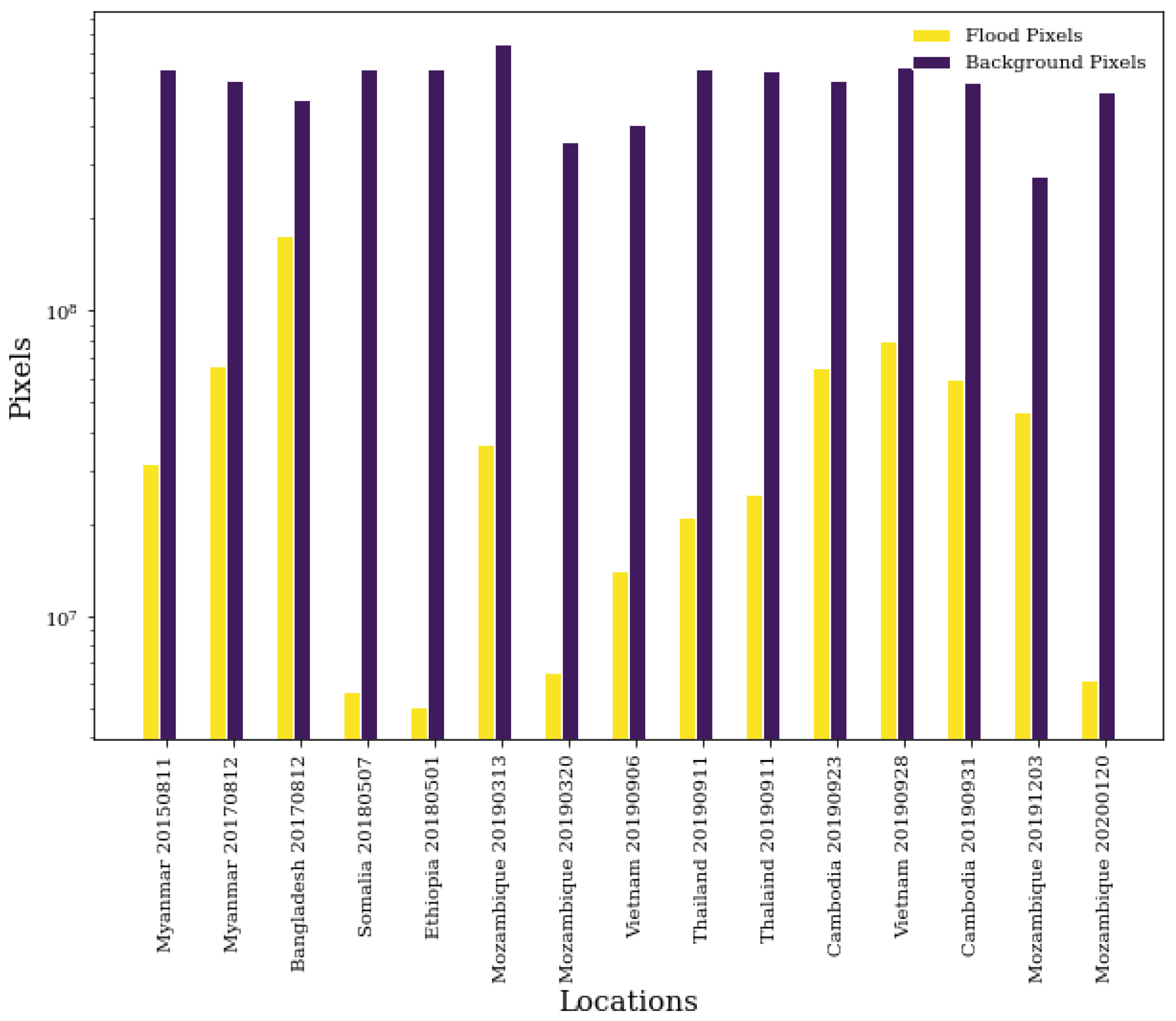
As shown in Table 2 and Figure 4, the dataset is also highly imbalanced with water pixels making up only 6% of the dataset. Such imbalances can have a significant effect on model performance due to the optimization strategies commonly used, and therefore we aim to mitigate this effect. In doing so, we under-sampled at the tile level by excluding all tiles that only contained background pixels. In order to maintain the structure of the tiles, under-sampling at the pixel level to reach a 50:50 ratio between classes was not possible. However, by performing tile under-sampling, the water to background pixel ratio was increased from 6% to 16% and also resulted in a training speed increase.
2.4. Automatic Histogram Based Method
2.5. Convolutional Neural Networks
Convolutional neural networks have been developed for many segmentation tasks, including several in remote sensing. We test various existing neural network architectures for flood identification and compare these against the method described in Section 2.2 and our baseline. Specifically we assess the performance of the well used U-Net model [64], and an alternative model, XNet [65].
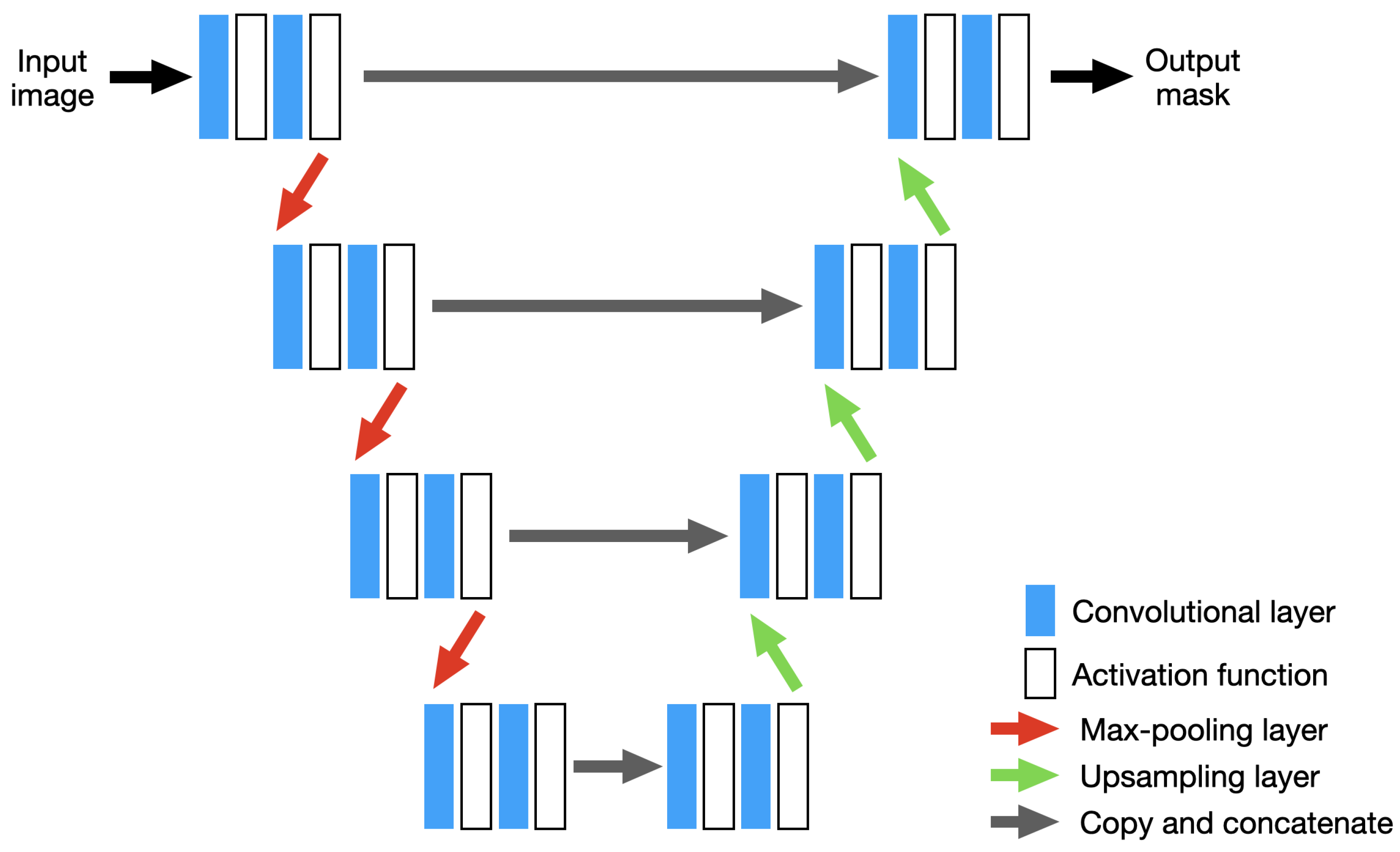
Both U-Net and XNet are convolutional neural networks consisting of encoder and decoder modules as well as utilizing weight sharing. The encoder module consists of a series of convolutional layers for feature extraction, along with max-pooling layers which downsample the input. The decoder is applied after feature extraction and performs upsampling to generate a segmentation mask of equal dimension to the input. The decoder also consists of further convolutional layers which allows for additional feature extraction and thus produces a dense feature map.
U-Net, shown in Figure 5, consists of an encoder for capturing context, and a symmetric decoder which allows for precise localization of features in the tile. The encoder consists of a stack of the convolutional layers followed by rectified liner unit (ReLU) activation functions to add non-linearity to the model, and max-pooling layers for downsampling. The decoder consists of convolutional and upsampling layers. Through using feature concatenation between each level, denoted “copy and concatenate” in Figure 5, precise pixel localization has been found to be enhanced [64]. Here, the feature maps saved during the downsamping/encoder stage are concatenated with the output of the convolution layers during the upsampling/decoder stage. Neither U-Net nor XNet contain any dense layers and therefore can accept tiles of any size.
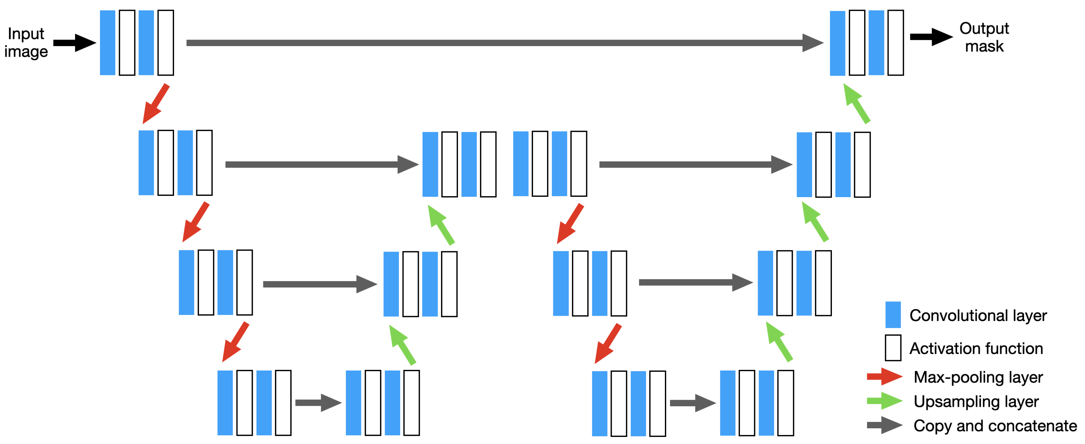
XNet, shown in Figure 6, consists of many of the same features contained in U-Net. However, instead of following the encoder-decoder structure shown in Figure 5, this architecture consists of a symmetric encoder-decoder-encoder-decoder structure. By containing multiple decoder stages alongside avoiding large serial downsampling of the input tile, XNet is designed to be sensitive to boundary level detail, particularly around small structures, while still achieving strong performance on largescale structures [65]. As with U-Net, XNet also leverages feature concatenation between encoder and decoder stages to help avoid the loss of important information between the downsampling and upsampling stages.
2.6. Transfer Learning
Transfer Learning is a machine learning method where a pre-trained model is used as a starting point for another model with a similar architecture. Using pre-trained models allows for the leveraging of previously learnt features, often on different datasets (which may help with generalizability), and can greatly speed up training and development time. Transfer learning is often used in applications where the labeled datasets are small, and training a neural network from scratch can be challenging due to its computational complexity.
Deep neural networks generally extract relevant information using a hierarchical approach. Initial layers detect high-level features such as corners and edges which are necessary for many image recognition problems, while the later layers detect more sophisticated features which are likely more domain specific. Due to this structure, neural networks are highly suited to transfer learning.
In the case of neural networks, a common approach is to alter the architecture of the model you wish to use such that part of it conforms to the design of another pre-trained model. The weights from the pre-trained model are then ported into the architecture you wish to train. Training of the entire architecture can then be performed, starting from the pre-trained weight values, or a subset of the model layers can be trained at different time steps. This latter method can help with model performance, as well as training speed.
In this study, we test the performance of training a U-Net style architecture as described above, but with the encoding/downsampling stage replaced with a ResNet architecture [66] which has been pre-trained on the ImageNet database [67] (see Figure 7). Since ResNet was originally designed for image classification, in order to connect the ResNet ‘backbone’ the classification layers has been removed such that all convolutional layers remain, but any flattening and dense layers for classification have been eliminated. By making this alteration, the modified ResNet architecture acts purely as a feature encoder in line with the encoder description provided in Section 2.5 and contains potentially useful information for high level feature extraction such as edge detection and general shape recognition.
2.7. Comparison Algorithms
We test a variety of automated algorithms and compare each performance against the method described in Section 2.2 for label generation. As a simple baseline to justify the use of more complex techniques, we use the automatic histogram based method described in Section 2.4. Here we minimize the mean squared-error between the labels and the output of the linear model applied after the necessary pre-processing steps.
Against this baseline we test several neural network architectures with different hyper-parameter values and compare their performance, while also accounting for the difference in training and testing time between the automatic histogram based method and the neural networks. We train XNet [65] and U-Net [64] architectures, both implemented in Keras [68] with a Tensorflow backend [69]. All input tiles are normalized prior to training and inference by applying mean subtraction and min/max scaling.
In addition, we test a transfer learning approach by training a U-Net architecture with a ResNet-34 [66] backbone structure implemented in the fastai library [70]. The model is trained using a one-cycle policy and fine-tuned using discriminative and slanted triangular learning rates [71]. Input tiles are normalized using ImageNet [67] statistics.
2.8. Computational Platform and Evaluation Criteria
We trained our models on Amazon Web Service (AWS) instances using NVIDIA Tesla K80 GPUs. The models were also tested using PulseSatellite, a collaborative satellite image analysis tool enabling HITL style model interaction, for compatibility and to test the possibility of deployment [51].
Given an input tile, the segmentation techniques described above assign a class to each pixel. In this study, a binary segmentation is performed and thus two outcomes are possible: positive or negative, which correspond respectively to water and background regions. The classifier output can be listed as:
- True Positive (TP): Water pixels correctly classified as water
- True Negative (TN): Background pixels correctly classified as background
- False Positive (FP): Background pixels incorrectly classified as water
- False Negative (FN): Water pixels incorrectly classified as background
There are a variety of metrics that can be used to evaluate the segmentation. For instance, pixel accuracy reports the percentage of pixels in the tiles that are correctly classified irrespective of their class. However, this metric can be misleading when the class of interest is poorly represented. To avoid this, precision, recall, the critical success index (CSI) (The CSI is equivalent to the intersection over union (IoU) of the water class) and F1 scores are commonly used [74,75,76]:
Precision is the fraction of relevant instances among the retrieved instances, i.e., it is the the ”purity” of the positive predictions relative to the labels. In other words, the precision illustrates how many of the positive predictions matched the labeled annotations. Recall is the fraction of the total amount of relevant instances that were actually retrieved, i.e., it describes the ”completeness” of the positive predictions relative to the labels. In other words, of all objects annotated in the labeled data, the recall denotes how many have been captured as positive predictions. As shown here, the F1 score is just the harmonic mean of the precision and recall and is equivalent to the dice similarity coefficient, thereby providing a metric which combines both the precision and recall statistics into one number. The CSI is also highly related to the F1 score and is provided here for clarity since it is a common metric to use in such mapping exercises. For a discussion on the similarities and trade offs of both the F1 and CSI metrics, see [76].
Besides the commonly used evaluation metrics for segmentation, it is relevant to also define the impact of this study in a broader context. Since rapid response is crucial during a humanitarian crisis, the time saved compared with using the methodology described in Section 2.2 is used as an impact metric. The time was calculated from when the image was initially accessed to the delivery of the final map (see Section 4.3).
2.9. Neural Network Hyper-Parameter Tuning
Given the variety of architectures being tested, as well as limited compute resources available, hyper-parameter tuning was carried out by manually varying parameters found to be particularly effective in improving model performance. If parameters were tested which did not have a significant impact on performance then these were sometimes not varied in later tests due to computational efficiency. Performance was measured using the precision, recall, CSI and F1 statistics presented in Equations (3)–(6).
For the case of the XNet and U-Net models, the learning rate was set to and varied by an order of magnitude with no immediate effect on performance. In the case of the U-Net+ResNet transfer learning approach, we utilized the fastai ‘learning rate finder’ tool to assist in choosing the learning rate for each training phase. Moreover, different ResNet depths (i.e., the number of skip-connection modules included in the backbone) were tested, although this too made minimal difference and so a smaller backbone was chosen for computational efficiency. The XNet and U-Net models were set to use a kernel size of 3 × 3 with a stride of 1, as a trade off between incorporating additional contextual information and memory efficiency, with the U-Net+ResNet kernel sizes and strides set to the default values.
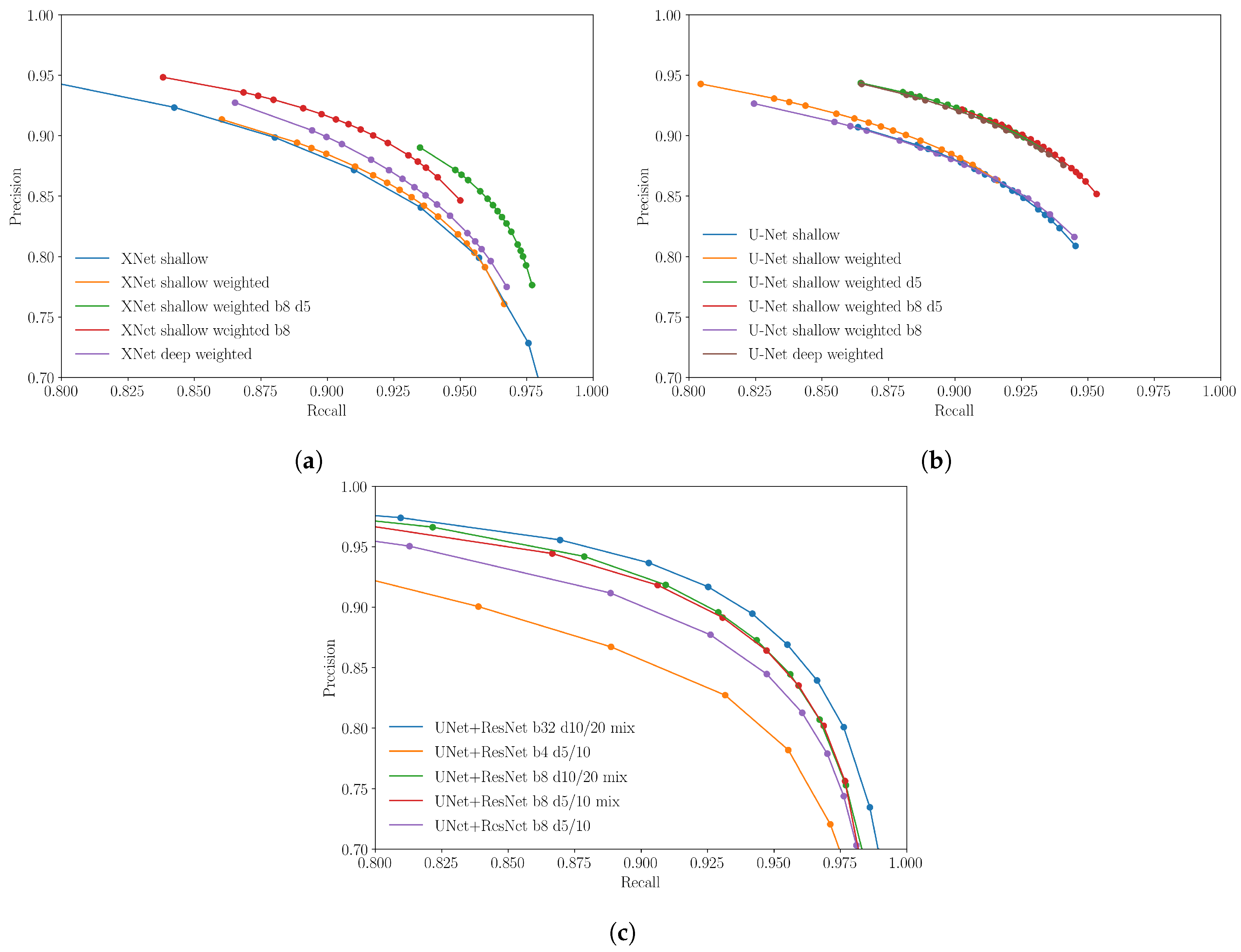
In Figure 8 we present results obtained by varying the batch size, number complete passes over the training set during model training, the use of a weighted loss function (giving greater weight to the flooded pixels in proportion to their imbalance in the dataset), changes in filter depths of the convolutional layers and the use of mixed precision during the training phase (i.e., the use of both 16 and 32-bit floating point numbers in the model during training). Details of the model setups are provided in Table 3 which also serves as a key for curves shown in Figure 8 and those shown subsequently.
Figure 8a,b show the performance of the XNet and U-net architectures with various hyper-parameter configurations. Two different filter depth configurations are tested: ‘deep’ and ‘shallow’, with the former being four times the size of the latter (see Table 3). Since we see that filter depth seems to have little effect on model performance in the ranges tested, for computational efficiency we assess the impact of the remaining hyper-parameters on models with smaller filter depths. When it comes to training the larger and more complex U-Net+ResNet model, we assume this depth variation to have similarly little effect and so did not assess its impact for this model. Here we take the default fastai filter depth sizes for both the U-Net and ResNet backbone.
When training the XNet and U-Net models, we test using both weighted and unweighted loss functions to account for the unbalanced dataset. This was also found to have minimal effects in comparison to other hyper-parameters and so we kept the weighted loss for the U-Net+ResNet model since we feel this may enable greater generalizability in future scenarios where datasets may be even more imbalanced.
Given the large size of the training dataset, when training the XNet and U-Net models, each epoch only passed over a fraction of the total training set. By default, we ensured the model is passed the same number of tiles as is contained in the training set once before Early Stopping is introduced. By increasing this to five passes we see that this can have a significant impact on model performance. This is to be expected given the diversity of the training set and the relatively few times the model is likely to see a given tile.
We discover mixed results when increasing the batch size from 3 to 8, with XNet performance increasing with the batch size and not increasing further with the number of passes over the dataset, whereas in the U-Net case the converse is found. In general we also do not see a significant difference in performance if one chooses to use either the XNet or U-Net architecture. Final testing to isolate the number of times a tile is shown to the model, and its batch size, is therefore only carried out on the U-Net architecture.
In Figure 8c we present the results for similar tests performed on the UNet+ResNet model which utilizes transfer learning. These curves show similar characteristics to those shown in Figure 8a,b and therefore suggests that the addition of transfer learning does not have a significant impact in this example. Another feature of testing carried out at this stage was the effectiveness of mixed precision. In general, using mixed precision is designed to decrease training time and has also been observed in certain circumstances to improve performance. Although the best performing model here has been trained with mixed precision, the differentiating factor from the other mixed precision models appears to be the number of times the whole training data is passed to the model during training, as well as some improvement coming from varying the batch size.
3. Results
3.1. Experimental Results
In this section we present the results of the different methodologies as applied to an unseen test set after hyper-parameter tuning. The test set was made up on 5813 tiles from across the different images and locations in the training set (see Section 2.3).
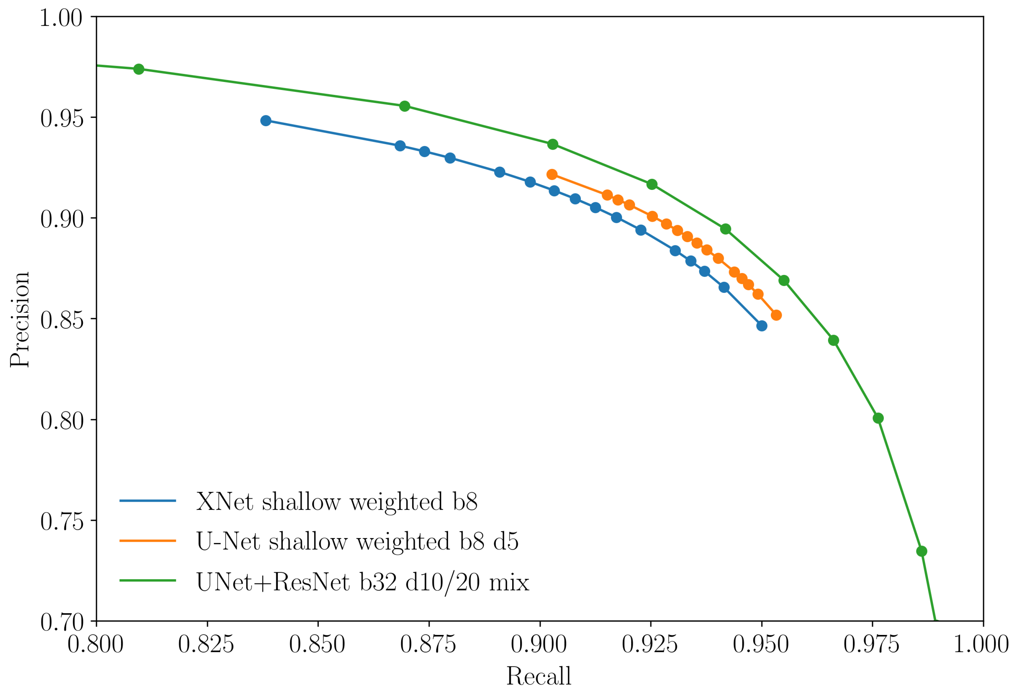
In Figure 9 we plot the best performing model for each of the three different architectures tested. While it should be noted that these curves are not wholly equivalent since the hyper-parameters chosen for one model inform those applied to the next, in Table 4 we can clearly see that the neural network based approaches significantly outperform the linear baseline. Higher precision suggests the neural network’s ability to identify a bigger proportion of correct positive identifications, thereby decreasing the number of pixels that an analyst would have to manually clean. Higher recall refers to a greater percentage of total relevant results correctly classified by the neural network.
For additional rigour, the F1 scores quoted in Table 4 are for the best threshold value according to model performance on the validation set as evaluated using the F1 score. Moreover, from these results we see that neural network approaches are also able to achieve strong performance in comparison to the labels created using the time consuming process described in Section 2.2.
While the models do not significantly differ in performance, the results presented in Figure 9 show that when using the U-Net+ResNet model, the choice of threshold can have a more significant effect on precision/recall statistics than in the case of the XNet and U-Net architectures. In most cases, the threshold producing the best F1 score might be chosen and so this threshold sensitivity may not be important. However, cleaning noise in a flood extent is easier than adding in missing flooded pixels and so a higher precision might be favourable (at the reasonable expense of recall). In order to allow for greater variability in the choice of precision/recall tradeoff, the U-Net+ResNet model may therefore be the most favourable, although the more computationally expensive.
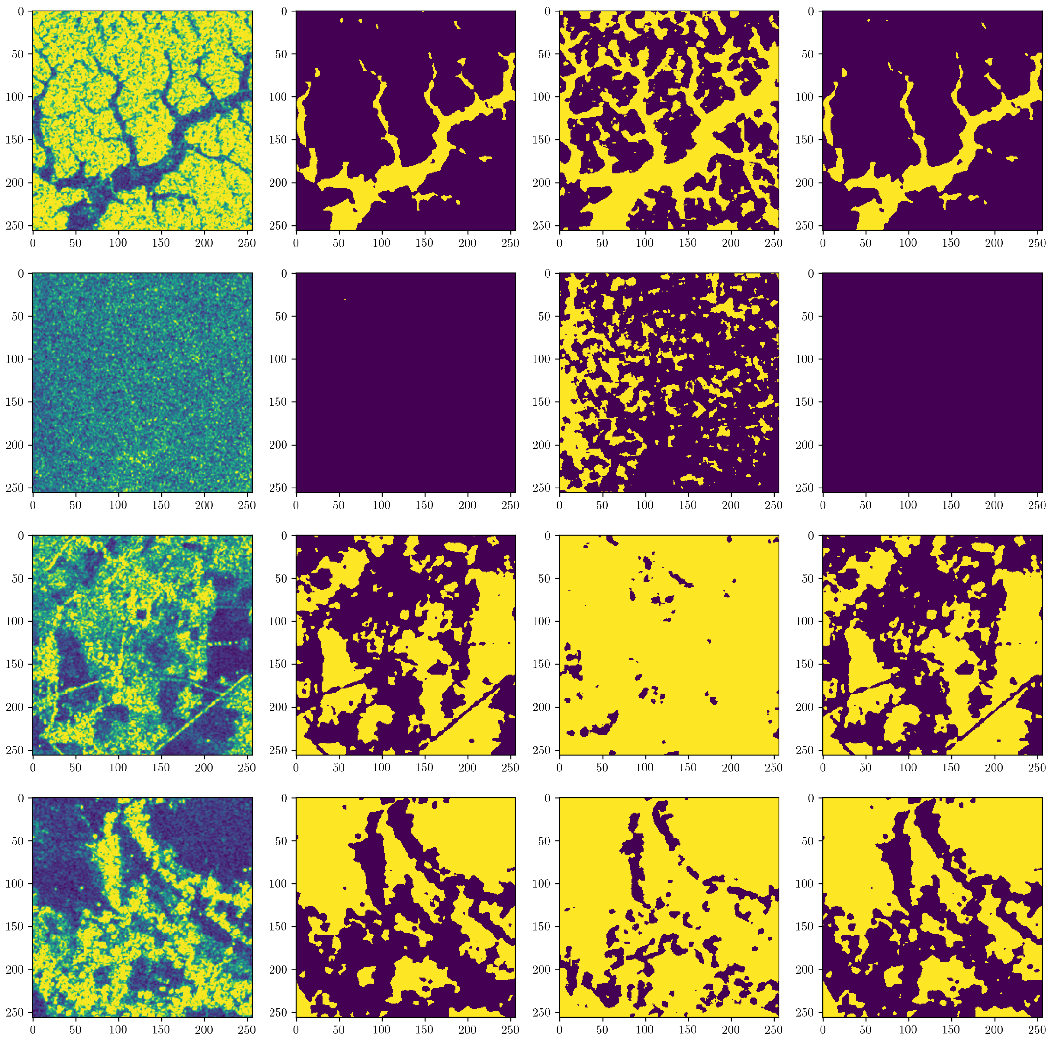
Example outputs of the best performing U-Net+ResNet, after probability thresholding, can be seen in Figure 10. In particular, we see the neural network’s ability to detect the flood area with little difference in comparison to the labeled data. The baseline (third column in Figure 10) was generated using the automatic threshold based method and would require significantly more noise reduction in post-processing. More examples of well detected tiles from both the baseline and this neural network, particularly highlighting severe flooded regions, can be seen in Appendix B.
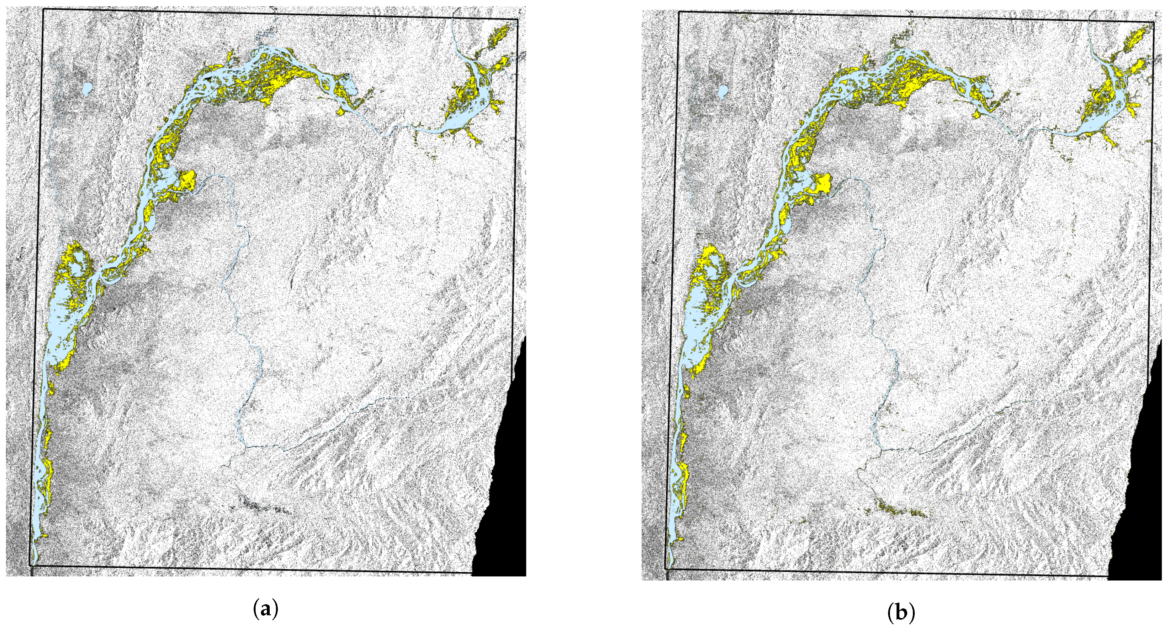
3.2. Sagaing Region—18 July 2019
To further test the generalizability of our model, we demonstrate performance on a set of tiles compiled from one completely unseen location. The U-Net+ResNet model was tested over the Sagaing Region, Myanmar on 18 July 2019. The image was downloaded by Copernicus Hub [53] and compared to the UNOSAT analysis (Shapefile and GeoDatabase with analysis extent over Sagaing are available at: https://www.unitar.org/maps/map/2921). In addition, to test how the model can be used in an operational fully-automated flood mapping setting, tests were performed to determine results both on overall water detection ability (as performed above) as well as only on the flooded regions. The Global Surface Water Dataset [77] was used to subtract permanent water from the model prediction which was then compared to the classically generated flood extent mask, thereby testing performance on the regions of greatest interest, i.e., just the flooded regions. A comparison of the model output to the labels can be found in Figure 11.
A common issue when performing CNN based image segmentation are border artifacts. We mitigate these by tiling the image with a stride less than the tile dimensions thereby ensuring overlap. In addition to this we clip the tiles to remove the exterior 2-pixels. In overlapping regions, we take the average of the inferred pixel values.
The results of this analysis are presented in Table 5. Here we see that the model performance on water detection is comparable to that presented on the test set in Table 4; however, performance on flood only regions is marginally lower. This is not necessarily surprising since the flooded regions may well present slightly different characteristics compared with combining all water bodies together as we did when creating labels for training the model. We also notice that the accuracy score changes little between the two comparisons since the background clearly dominates in this example, therefore presenting a good test of the model’s ability to detect ‘no flood’ in background-only tiles. During previous training, validation and testing, background-only tiles were removed to better balance the datasets, and reduce training time. In the example presented here, these tiles have not been removed since they would be unknown in an operational context, but we can see that this does not significantly affect the performance.
4. Discussion
4.1. Comparison to the Literature
As shown above, we compare various neural network methodologies for the detection of flooded pixels in SAR imagery. In doing so, performance is measured against commonly used classical techniques [21,54,55,56,57], followed by extensive manual cleaning and visual inspection, which were used to generate labeled data for training, validation and testing. Moreover, we designed an automated version of these classical methods against which we benchmark our performance. By building this automated benchmark, which essentially acts as a linear model, we aim to justify the development of a more complex approach, such as that of a neural network.
As can be seen in Table 4, the neural network approaches greatly outperform the baseline automated method, while also achieving F1 scores above the 92% level averaged over the entire testing dataset. Indeed, since this performance is achieved over a significantly large dataset with different land formations, we demonstrate the generalizabiility of our approach to different environmental conditions. Furthermore, in Section 3.2 we provide an analysis of model performance on tiles from a completely unseen image and location. In this case, Table 5 demonstrates further strong performance against the classically created labels, both on total water detection, as well as flood specific detection.
As discussed in the Introduction, Zhang et al. [49] and Kang et al. [50] both develop CNNs for water detection in SAR imagery. These studies focus on a relatively small selection of regions and have been trained on water masks generated by hand, rather than benchmarking against the more detailed classically generated masks with manual cleaning such as those presented in this paper. In comparison to the results presented in these studies, our model shows similar or better performance. Specifically, Kang et al. achieve F1 scores of between 0.90 and 0.94 per location, with 0.90 being achieved on their totally independent image (Study 3), as opposed to the 0.95 achieved in our example. Comparing with Zhang et al. is more challenging since their methodology was developed for water and shadow identification. However, their overall accuracy achieved on studies with reasonable mean intersection of unions (MIoUs) is in the region of 88–91%, thus scoring lower than our methodology.
As mentioned previously, further to our method being comparable, or performing better than, previous related works, we also make an explicit check on our model’s ability to classify flood-only pixels, as opposed to all water bodies in an image. We think this analysis is essential since achieving strong metrics on flood specific detection is the key task required during operational rapid mapping. Indeed, while we agree with the issues raised in [50], surrounding previous studies not using independent imagery for testing and comparison, we propose a further recommendation that future modelling investigations present performance of their techniques on both general water detection, as well as specifically quoting metrics for flood-only detection (i.e., all water detected minus permanent water bodies).
While we show strong performance against existing methodologies of flood detection using solely SAR imagery, our results are also comparable to, and in several cases outperform, machine learning methods that require the use of optical imagery. Specifically, the works of Mateo-Garcia et al. [33] and Benoudjit et al. [40] use a set up comparable to ours, since they use the same label generation techniques but without the additional manual cleaning and visual inspection that we perform to improve the quality of our training data. In the former, the authors achieve F1 scores between 0.80–0.88 depending on the resolution of the images in the dataset, whereas in the latter the authors achieve F1 scores between 0.73–0.90 depending on the environment being tested. Again, the results presented in Table 4 demonstrate that our methodology produces similar or better scores on comparable flood maps without the need for optical data.
4.2. Applications to Humanitarian Situations, Disaster Relief and Rapid Mapping Services
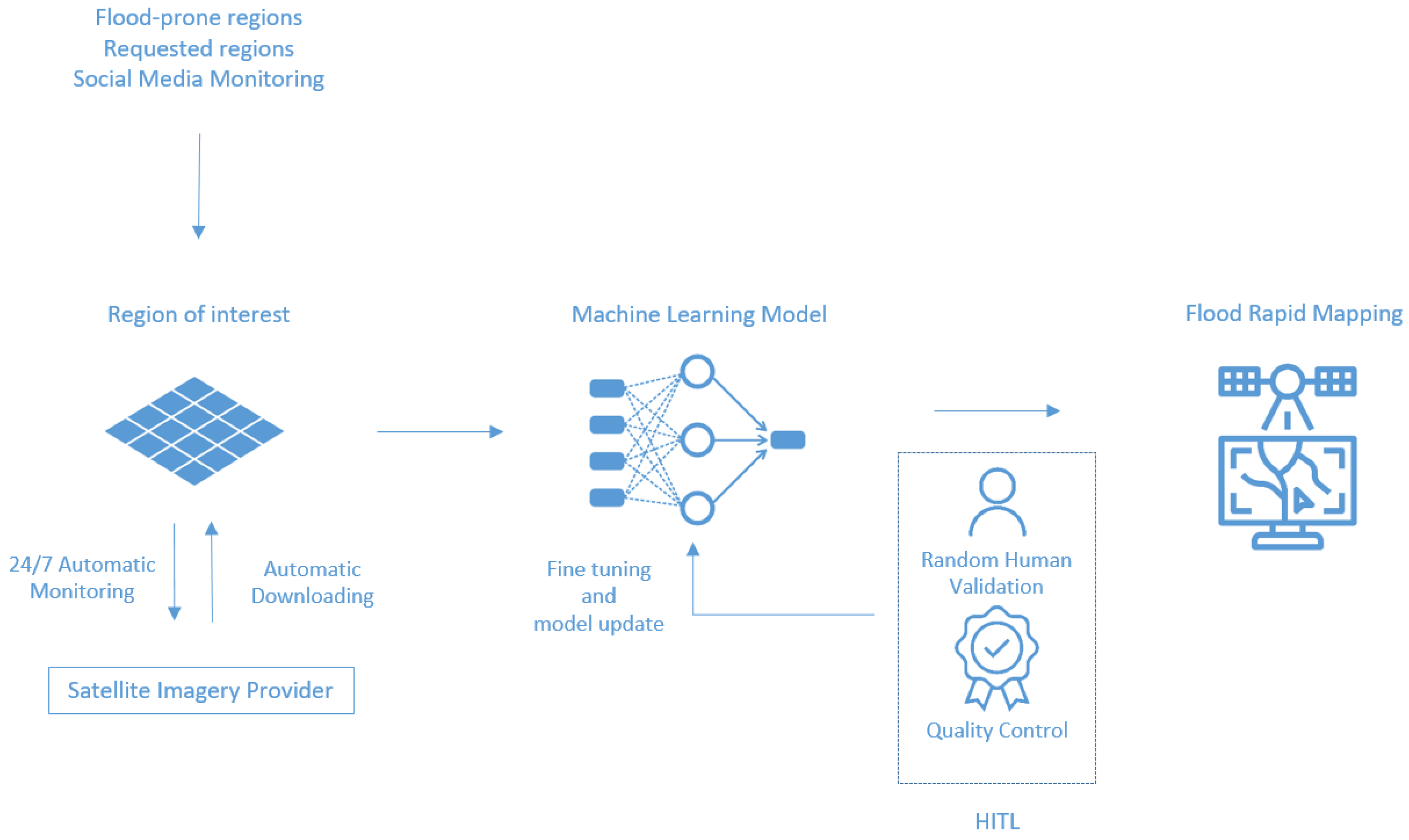
Given these promising results, a fully automated pipeline similar to that of [25] can be implemented whereby images of flood-prone areas are automatically downloaded and processed to output disaster maps. Such an automatic AI-based flood mapping workflow could download and pre-process SAR imagery from data sources such as the Copernicus Hub and feed this into a neural network that outputs a flood segmentation mask. This tool would potentially allow for query, download, and pre-processing of Sentinel-1 imagery through an interface that communicates with the Scihub Copernicus platform [53], and ESA SNAP [78], a desktop software used for pre-processing satellite images. A possible configuration of such an automatic pipeline is shown in Figure 12.
Additionally, such models can be integrated into human-in-the-loop (HITL) systems for random validation testing and iterative model performance enhancement, such as that presented by Logar et al. [51]. By utilizing such systems, if there is a location in which the model is failing then expert analysis can be fed back into the model either to fine-tune it to the specific situation at hand, or to generally increase model performance by expanding the training set. In these circumstances, since the model would not necessarily be required to be completely retrained [3], this procedure can be a relatively inexpensive process.
As highlighted previously, one of the significant advantages of this study is that the models have been trained and tested on flood masks generated from operational rapid mapping response scenarios which represent the desired outcome to be reproduced. Since the results presented here demonstrate high metric scores across a wide range of locations, and have specifically shown the ability to generalize to tiles from completely unseen images and locations, with appropriate validation and checks, our method has been deemed appropriate by experts for testing in disaster response situations. Moreover, one of the crucial bottlenecks in humanitarian disaster response is the time between requests for analysis and the final result. While we shall discuss the speed up gained through using a neural network based approach in the next section, it should also be noted that such an automated system would allow for 24/7 monitoring and surveillance. In such instances, partner organisations could make map requests and receive a rapid response without analysts needing the ability to respond immediately. Since emergency responders need timely information as fast as possible when responding to disaster situations, such a system could translate into numerous lives saved.
4.3. Cost Effectiveness Analysis
The financial implications of analysis is of great importance to organisations undertaking rapid mapping, as they are are often operating on tight and restricted budgets. We perform a Cost Effectiveness Analysis (CEA) comparing the widely used threshold method with the solutions presented in this paper. A CEA is a ’type of value-for-money analysis that compares the relative costs of different alternatives that achieve different amounts of the same impact’ [79]. CEA is often used in the health sector where it is inappropriate to associate an economic value to human life. The output of the analysis is expressed in terms of the Effectiveness-Cost ratio (EC ratio) between affected people and total cost. The methodology with the highest EC ratio is the most effective, and therefore affects a greater number of people for each cost unit. Three methodologies were compared: the histogram based method as followed by an expert analyst, the automatic histogram based method used as baseline, and the U-Net+ResNet neural network based approach (which is the most computationally expensive of the three architectures to train and perform validation on).
Firstly, the time of each activity, shown in Table 6, must be monitored in order to quantify the cost of each methodology. The personnel costs are based on the salary for a UN GIS analyst and a UN GIS senior analyst, are set respectively at $26 per hour and $44 per hour according to the United Nations Remuneration Rate [80]. Other costs, i.e., electricity, administration, computational, and others are not taken into account. Using a histogram based method requires 6 h for the UN GIS analysis to download and process the image and 1 h for the UN GIS senior analyst to perform quality control. By using a single GPU, the automatic histogram based method requires 30 min for automatic download and pre-processing, 5 min for segmentation by the algorithm and 2 h for the quality control and cleaning. The neural network approach, however, requires only 20 minutes for the automatic download and pre-processing since less of the latter was found to be required. Tiling and inference takes 5 min and final quality control, if needed, can take up to 1 hour. Therefore the entire workflow for this methodology requires 1 hour and 25 min with a UN GIS senior analyst only becoming involved at the quality control stage.
The number of ‘affected people’ was calculated by studying a Bangladesh analysis that occurred on 12 August 2017 with the zonal statistics. Here, the number of affected people was set to 1,432,222 supposing a scenario of a severe flood event. Based on these assumptions, the EC ratio is computed for each methodology as shown in Table 7.
Using the automatic histogram based method or a neural network for flood segmentation will decrease the cost by 65% and 78% respectively, and the overall time needed for delivering a map by 63% and 80% as compared to existing workflows employed at agencies such as UNOSAT. However, using a neural network has a higher effectiveness concerning the number of people affected per unit currency. Specifically, with one single dollar, the neural network approach could potentially impact 360% more people compared to the current approach.
The Cost Effectiveness Analysis shows that both of the automated approaches are cheaper and less time-consuming. However, the effectiveness of a methodology during a natural disaster also relies on the ability to provide more updates during the same time period, which can be delivered by the neural network based method. The latter does not require any human intervention, beside a potential quality check, allowing the technology to be scalable to a 24/7 monitoring system. Moreover, such technology provides better results compared to the other methodologies analyzed.
4.4. CO2 Emission Related to Experiments and Deployment
This section aims for transparency on the CO2 emission of the experiments and to start a conversation on how to prevent unnecessary experiments and compensate for such emissions. Experiments were conducted using Amazon Web Services in region us-east-2, which has a carbon efficiency of 0.57 kgCO2eq/kWh. A cumulative of 1894 hours of computation was performed on hardware of type Tesla K80 (TDP of 300 W). Total emissions are estimated to be 323.87 kgCO2eq of which 0 percents were directly offset by the cloud provider. Estimations were conducted using the Machine Learning Impact calculator presented in [81].
A CO2 compensation should be considered during any production phase, such as a 24/7 monitoring platform, which will contribute an estimated total emission of 0.51 kgCO2eq a day considering that only the inference part is done on the cloud and by keeping all 24/7 monitoring to local machines. A CO2 compensation strategy is currently under investigation in order to deploy a zero net emission model for all intensive image analysis and remote sensing procedures. We encourage others to carefully monitor future CO2 emission related to experiments and deployments of artificial intelligence technologies.
4.5. Further Research
This research study focused on the development of flood segmentation techniques and exploring how these might be integrated into a fully automated pipelines (as discussed in Section 4.2). However, to enhance the impact of the AI-based methodology in the local communities affected by natural disasters, a technological and social partnership is needed. Protocols must be put in place between the data providers and the end beneficiaries in order to minimize unnecessary and costly procedures in the disaster relief chain [82].
Social media monitoring for flood events [83,84,85], real time events and risk detection platforms [86] has been shown to be effective in producing relevant alerts for disaster response. Such technology could be integrated prior to data acquisition to localize where the disaster occurs and automatically trigger the generation of a flood map. Timely information and image acquisition could therefore leverage the speed of the AI-based method and its potential independence from human intervention. It would also reduce the time needed to report the event to the relevant organizations leading to faster humanitarian support.
In addition to finding new ways to augment the processing pipeline for rapid response, we encourage others to test the generalizability of this approach across even more landscapes and situations, as well as perform testing on data generated using different classical water detection techniques beyond those presented in Section 2.2. Since the masks used here for model training and testing were generated in situations requiring rapid response to disaster situations, field-level feedback was not incorporated into the mapping process. A future line of research could be to train a model on data generated in collaboration with field operations, which is highly expensive to collect, but could be used to produce a model of an equivalent standard, thus potentially surpassing current classical methodologies in terms of thematic accuracy.
5. Conclusions
The ability to perform rapid mapping in disaster situations is essential to assisting national and local governments, NGOs and emergency services, enabling information to be gathered over large distances and visualised for planned response. Non-governmental, national and international agencies currently spend many hours, using a variety of manual and semi-automated classical image processing techniques, resulting in highly detailed maps of flood extent boundaries.
In this work we present a machine learning based approach to further automate and increase the speed of rapid flood mapping processes, while achieving sufficiently good performance metrics for deployment across a broad range of environment landscapes and conditions. By using convolutional neural networks trained on a wide variety of flood maps created using SAR imagery, we are able to produce results which are comparable, or outperform, previous more limited studies of SAR flood segmentation, as well as methods which also include the use of optical imagery not required by our methodology. In addition, our approach requires minimal pre-processing before the image is fed into the network, thereby speeding up inference time, and does not rely on many additional external data sources.
In this work, we not only demonstrate model performance over a wide ranging, diverse dataset of images taken from some of the most disaster prone areas of the world, but also explicitly present statistics on both unseen tiles gained from images that have been partially seen by the model, as well as unseen tiles derived from completely unseen images. Furthermore, we assess model performance on the usual analysis task of water detection, as has been carried out in previous studies, as well as specifically focusing on the model’s ability to detect new flooded regions which are additional to the permanent water in the image. Building on previous recommendations, such as those by Kang et al. [50], we hope future studies also take a similar approach to assessing model performance rather than solely focusing on water detection.
Through using a machine learning based approach there is also potential to increase the impact to end beneficiaries during humanitarian assistance by allowing for the implementation of live streaming mapping services triggered by direct partner requests or automatic activations. By enabling flood mapping to be completed automatically in a fraction of the time, teams on the ground are able to respond more quickly to disaster situations.
Using the existing histogram based method, a flood map can be provided in 24 h; however, floods change quickly thereby rapidly rendering maps outdated. Additionally, because an analyst takes many hours to producing a flood map, the frequency with which maps can be created is limited to the number of analysts. By using the method presented in this paper, flooded regions can be identified in a significantly shorter time period using fully automated methods, allowing the dissemination of more timely information and enabling new workflows to be developed.
Rapid flood mapping is a crucial source of information, and a speed up in this process could have extremely meaningful repercussions for disaster response procedures.
Author Contributions
Conceptualization, L.B. and J.B.; Methodology, E.N, J.B. and S.B.; Software, E.N. and J.B.; Validation, E.N, J.B., S.B. and L.B.; Formal Analysis, E.N. and J.B.; Investigation, E.N., J.B., S.B. and L.B.; Resources, E.N., J.B., L.B. and S.B.; Data Curation, E.N. and S.B.; Writing—Original Draft Preparation, E.N. and J.B.; Writing—Review and Editing, E.N., J.B., S.B. and L.B.; Visualization, E.N. and J.B.; Supervision, E.N., J.B., L.B. and S.B.; Project Administration, L.B.; Funding Acquisition, J.B. and L.B. All authors have read and agree to the published version of the manuscript.
Funding
E.N., L.B. and S.B. are with the United Nations Institute for Training and Research’s (UNITAR) Operational Satellite Applications Programme (UNOSAT) supported by the Norwegian Agency for Development Cooperation concerning rapid mapping and disaster response. J.B. is with the United Nations Global Pulse innovation initiative supported by the Governments of Sweden, Netherlands and Germany and the William and Flora Hewlett Foundation. J.B. is also supported by the UK Science and Technology Facilities Council (STFC) grant number ST/P006744/1.
Acknowledgments
This project has received access to public cloud services from the CERN openlab, a public-private partnership through which CERN collaborates with leading ICT companies and other research organisations. J.B. is also grateful for the support of the Institute for Data Science (IDAS) and the Institute for Particle Physics Phenomenology (IPPP), both at Durham University, UK. All the authors thank UNOSAT Geospatial Analysts in Geneva and Bangkok office for their crucial support. We thank Vanessa Guglielmi, Jakrapong Tawala, Teodoro Hunger, and Jialin Yan for the creation and revision of the dataset. We thank Teodoro Hunger and Sami Tabbara for the support on the analysis over Sagaing Region and the work done on the operational fully-automated pipeline respectively. We thank João Fernandes, Sofia Vallecorsa, Ignacio Peluaga Lozada, Marion Devouassoux, and Dominique Cressatti from CERN IT Department for providing access to the IT infrastructure and for the constant support provided from the beginning of this project. We thank Tomaz Logar for help with technical implementation and Einar Bjorgo and Miguel Luengo-Oroz for continuing guidance and support throughout this project.
Conflicts of Interest
The authors declare no conflict of interest and the funders had no role in the design of the study; in the collection, analyses, or interpretation of data; in the writing of the manuscript, or in the decision to publish the results.
Abbreviations
The following abbreviations are used in this manuscript:
| AWS | Amazon Web Service |
| AI | Artificial Intelligence |
| CEA | Cost Effectiveness Analysis |
| CNNs | Convolutional Neural Networks |
| CSI | Critical Success Index |
| EC | Effectiveness-Cost |
| ESA | European Space Agency |
| DEM | Digital Elevation Model |
| FP | False Positive |
| FN | False Negative |
| FCN | Fully Convolutional Network |
| GRD | Ground Range Detected |
| HITL | Human-in-the-loop |
| IoU | Intersection of Union |
| IW | Wide Swath |
| MIoU | Mean Intersection of Union |
| NGO | Non Profit Organisation |
| NDWI | Normalized Difference Water Index |
| NRT | Near Real Time |
| ReLU | Rectified Linear Unit |
| SAR | Synthetic Aperture Radar |
| TP | True Positive |
| TN | True Negative |
| UN | United Nations |
| UNITAR-UNOSAT | United Nations Institute for Training and Research Operational Satellite Applications Programme |
Appendix A. Copernicus Imagery

Table A1.
Location, event date, image name that can be download from the Copenicus Open Access Hub [53].
Table A1.
Location, event date, image name that can be download from the Copenicus Open Access Hub [53].
| Location | Event Date | Image Name |
|---|---|---|
| Myanmar | 11 August 2015 | S1A_IW_GRDH_1SSV_20150811T114721_20150811T114746_007215_009DE4_C4E2.tif |
| Myanmar | 08 May 2016 | S1A_IW_GRDH_1SSV_20160805T114607_20160805T114632_012465_0137A7_ACBC.tif |
| Bangladesh | 12 August 2017 | S1A_IW_GRDH_1SDV_20170812T235532_20170812T235557_017897_01E03B_AF9D.tif |
| Somalia | 01 August 2018 | S1A_IW_GRDH_1SDV_20180501T025444_20180501T025509_021705_025710_8835.tif |
| Ethiopia | 07 May 2018 | S1B_IW_GRDH_1SDV_20180507T151605_20180507T151630_010817_013C63_C906.tif |
| Mozambique | 13 March 2019 | S1A_IW_GRDH_1SDV_20190313T161522_20190313T161557_026321_02F156_A8A9.tif |
| Mozambique | 20 March 2019 | S1A_IW_GRDH_1SDV_20190320T160818_20190320T160843_026423_02F51E_5018.tif |
| Vietnam | 06 September 2019 | S1A_IW_GRDH_1SDV_20190906T110524_20190906T110549_028900_0346B3_457F.tif |
| Thailand | 11 September 2009 | S1A_IW_GRDH_1SDV_20190911T111310_20190911T111335_028973_034937_0BA8.tif |
| Thailand | 11 September 2009 | S1A_IW_GRDH_1SDV_20190911T111245_20190911T111310_028973_034937_C91D.tif |
| Cambodia | 23 September 2019 | S1A_IW_GRDH_1SDV_20190923T111155_20190923T111220_029148_034F2E_9682.tif |
| Vietnam | 28 September 2019 | S1B_IW_GRDH_1SDV_20190928T224435_20190928T224504_018244_0225A5_DC47.tif |
| Cambodia | 31 September 2019 | S1A_IW_GRDH_1SDV_20190927T225300_20190927T225325_029213_03516D_B4A3.tif |
| Mozambique | 03 December 2019 | S1A_IW_GRDH_1SDV_20191203T030914_20191203T030939_030178_0372DB_368F.tif |
| Mozambique | 20 January 2020 | S1B_IW_GRDH_1SDV_20200120T160700_20200120T160729_019902_025A5F_CDF4.tif |
| Sagaing Region | 18 July 2019 | S1A_IW_GRDH_1SDV_20190718T233107_20190718T233132_028178_032ED3_94DF.tif |
| Sagaing Region | 18 July 2019 | S1A_IW_GRDH_1SDV_20190718T233132_20190718T233157_028178_032ED3_6748.tif |
Appendix B. Tile Results
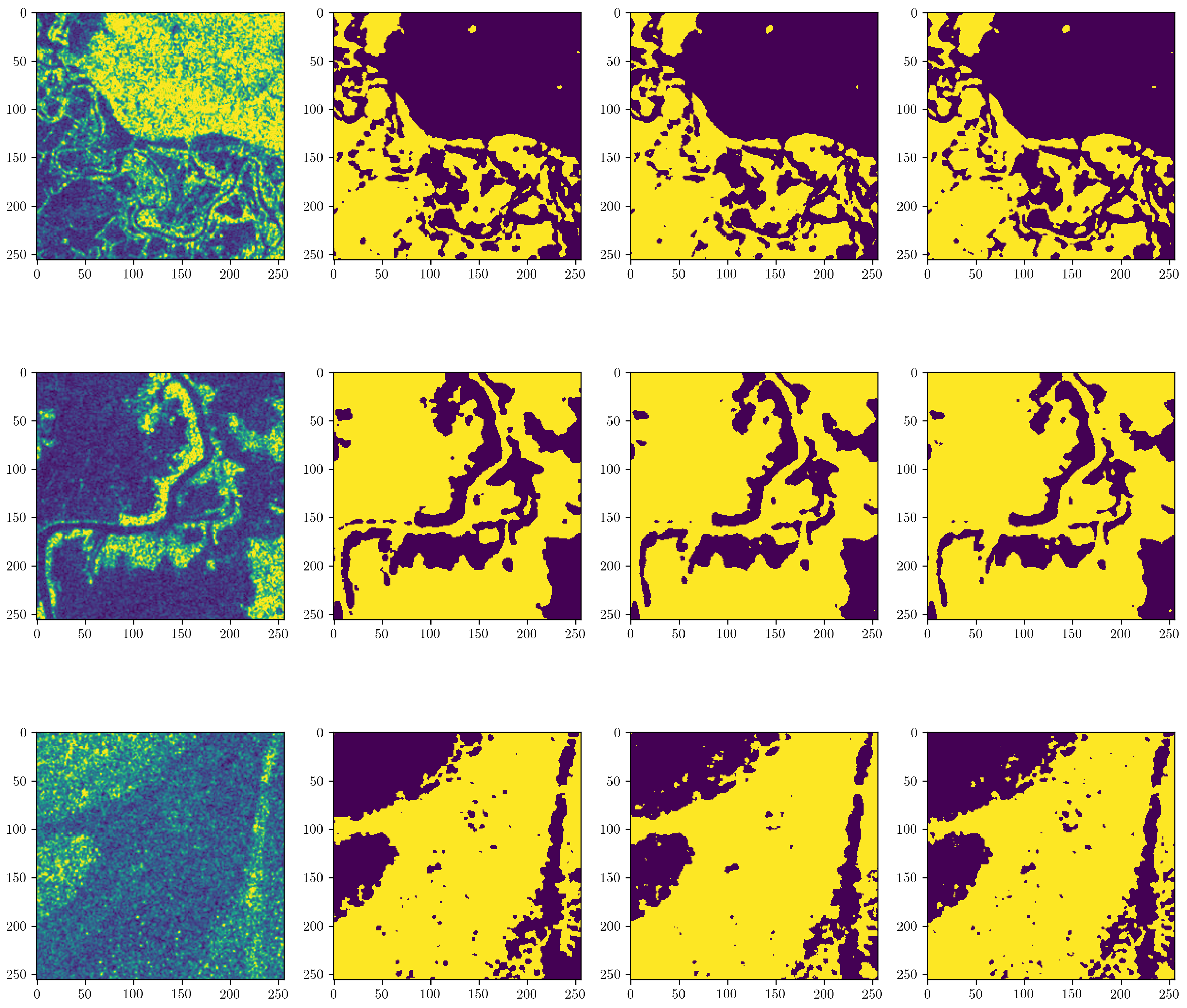
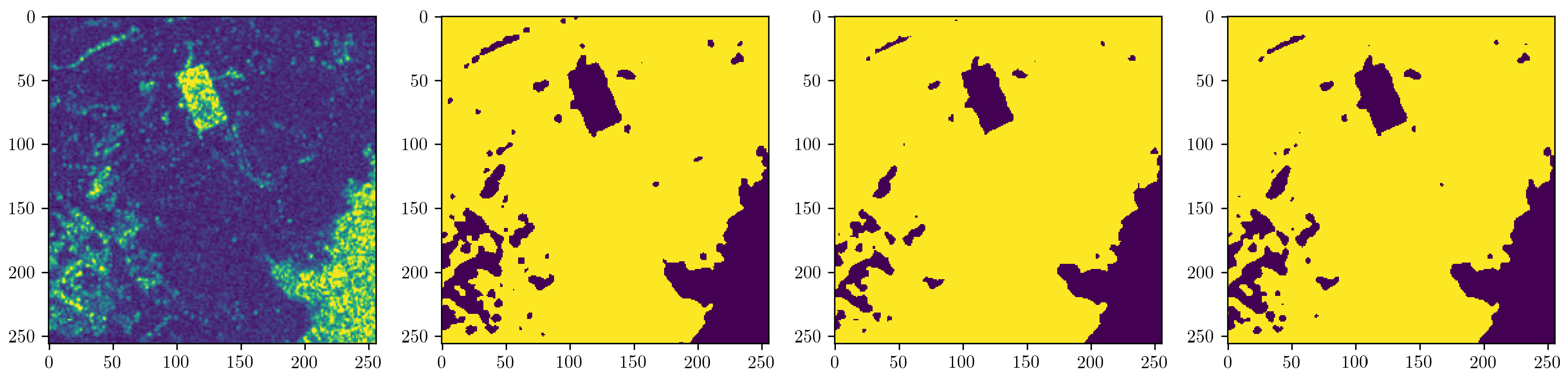
Figure A1.
From left to right: raw SAR tiles using the viridis colormap followed by tiles of different analyses esponding to classical histogram based, baseline and neural network predictions. The background is displayed in purple and flood in yellow.
Figure A1.
From left to right: raw SAR tiles using the viridis colormap followed by tiles of different analyses esponding to classical histogram based, baseline and neural network predictions. The background is displayed in purple and flood in yellow.


References
- Centre for Research on the Epidemiology of Disasters. The Human Cost of Weather-Related Disasters 1995–2015; United Nations Office for Disaster Risk Reduction: Geneva, Switzerland, 2015. [Google Scholar]
- Swiss, R. Flood—An Underestuimated Risk: Inspect, Inform, Insure. Available online: https://media.swissre.com/documents/Flood.pdf (accessed on 4 August 2020).
- Quinn, J.A.; Nyhan, M.M.; Navarro, C.; Coluccia, D.; Bromley, L.; Luengo-Oroz, M. Humanitarian applications of machine learning with remote-sensing data: Review and case study in refugee settlement mapping. Philos. Trans. R. Soc. A Math. Phys. Eng. Sci. 2018, 376, 20170363. [Google Scholar] [CrossRef] [PubMed] [Green Version]
- Serpico, S.B.; Dellepiane, S.; Boni, G.; Moser, G.; Angiati, E.; Rudari, R. Information Extraction From Remote Sensing Images for Flood Monitoring and Damage Evaluation. Proc. IEEE 2012, 100, 2946–2970. [Google Scholar] [CrossRef]
- Schumann, G.; Brakenridge, G.; Kettner, A.; Kashif, R.; Niebuhr, E. Assisting Flood Disaster Response with Earth Observation Data and Products: A Critical Assessment. Remote Sens. 2018, 10, 1230. [Google Scholar] [CrossRef] [Green Version]
- UNITAR’s Operational Satellite Applications Programme—UNOSAT. Rapid Mapping Service. Available online: https://www.unitar.org/maps/unosat-rapid-mapping-service (accessed on 4 August 2020).
- McFeeters, S.K. The use of the Normalized Difference Water Index (NDWI) in the delineation of open water features. Int. J. Remote Sens. 1996, 17, 1425–1432. [Google Scholar] [CrossRef]
- Rogers, A.; Kearney, M. Reducing signature variability in unmixing coastal marsh Thematic Mapper scenes using spectral indices. Int. J. Remote Sens. 2004, 25, 2317–2335. [Google Scholar] [CrossRef]
- Ji, L.; Zhang, L.; Wylie, B. Analysis of Dynamic Thresholds for the Normalized Difference Water Index. Photogramm. Eng. Remote Sens. 2009, 75, 1307–1317. [Google Scholar] [CrossRef]
- Memon, A.A.; Muhammad, S.; Rahman, S.; Haq, M. Flood monitoring and damage assessment using water indices: A case study of Pakistan flood-2012. Egypt. J. Remote Sens. Space Sci. 2015, 18, 99–106. [Google Scholar] [CrossRef] [Green Version]
- Moreira, A.; Prats-Iraola, P.; Younis, M.; Krieger, G.; Hajnsek, I.; Papathanassiou, K.P. A tutorial on synthetic aperture radar. IEEE Geosci. Remote Sens. Mag. 2013, 1, 6–43. [Google Scholar] [CrossRef] [Green Version]
- Covello, F.; Battazza, F.; Coletta, A.; Lopinto, E.; Fiorentino, C.; Pietranera, L.; Valentini, G.; Zoffoli, S. COSMO-SkyMed an existing opportunity for observing the Earth. J. Geodyn. 2010, 49, 171–180. [Google Scholar] [CrossRef] [Green Version]
- Werninghaus, R. TerraSAR-X mission. In SAR Image Analysis, Modeling, and Techniques VI; Posa, F., Ed.; International Society for Optics and Photonics: Bellingham, WA, USA, 2004; Volume 5236, pp. 9–16. [Google Scholar] [CrossRef]
- Mason, D.; Giustarini, L.; Garcia-Pintado, J.; Cloke, H. Detection of flooded urban areas in high resolution Synthetic Aperture Radar images using double scattering. Int. J. Appl. Earth Obs. Geoinf. 2014, 28, 150–159. [Google Scholar] [CrossRef] [Green Version]
- Chini, M.; Pulvirenti, L.; Pierdicca, N. Analysis and Interpretation of the COSMO-SkyMed Observations of the 2011 Japan Tsunami. IEEE Geosci. Remote Sens. Lett. 2012, 9, 467–471. [Google Scholar] [CrossRef]
- Pulvirenti, L.; Chini, M.; Pierdicca, N.; Boni, G. Use of SAR Data for Detecting Floodwater in Urban and Agricultural Areas: The Role of the Interferometric Coherence. IEEE Trans. Geosci. Remote Sens. 2016, 54, 1532–1544. [Google Scholar] [CrossRef]
- Chaabani, C.; Chini, M.; Abdelfattah, R.; Hostache, R.; Chokmani, K. Flood Mapping in a Complex Environment Using Bistatic TanDEM-X/TerraSAR-X InSAR Coherence. Remote Sens. 2018, 10, 1873. [Google Scholar] [CrossRef] [Green Version]
- Chini, M.; Pelich, R.; Pulvirenti, L.; Pierdicca, N.; Hostache, R.; Matgen, P. Sentinel-1 InSAR Coherence to Detect Floodwater in Urban Areas: Houston and Hurricane Harvey as A Test Case. Remote Sens. 2019, 11, 107. [Google Scholar] [CrossRef] [Green Version]
- Rudner, T.G.J.; Rußwurm, M.; Fil, J.; Pelich, R.; Bischke, B.; Kopacková, V.; Bilinski, P. Multi3Net: Segmenting Flooded Buildings via Fusion of Multiresolution, Multisensor, and Multitemporal Satellite Imagery. In Proceedings of the AAAI Conference on Artificial Intelligence, Honolulu, HI, USA, 27 January–1 February 2019; 2019; Volume 33, pp. 702–709. [Google Scholar]
- Pierdicca, N.; Pulvirenti, L.; Boni, G.; Squicciarino, G.; Chini, M. Mapping Flooded Vegetation Using COSMO-SkyMed: Comparison With Polarimetric and Optical Data Over Rice Fields. IEEE J. Sel. Top. Appl. Earth Obs. Remote Sens. 2017, 10, 2650–2662. [Google Scholar] [CrossRef]
- Chini, M.; Hostache, R.; Giustarini, L.; Matgen, P. A Hierarchical Split-Based Approach for Parametric Thresholding of SAR Images: Flood Inundation as a Test Case. IEEE Trans. Geosci. Remote Sens. 2017, 55, 6975–6988. [Google Scholar] [CrossRef]
- Martinis, S.; Kersten, J.; Twele, A. A fully automated TerraSAR-X based flood service. ISPRS J. Photogramm. Remote Sens. 2015, 104, 203–212. [Google Scholar] [CrossRef]
- Pulvirenti, L.; Pierdicca, N.; Chini, M.; Guerriero, L. An algorithm for operational flood mapping from Synthetic Aperture Radar (SAR) data using fuzzy logic. Nat. Hazards Earth Syst. Sci. 2011, 11, 529–540. [Google Scholar] [CrossRef] [Green Version]
- Mason, D.C.; Davenport, I.J.; Neal, J.C.; Schumann, G.J.; Bates, P.D. Near Real-Time Flood Detection in Urban and Rural Areas Using High-Resolution Synthetic Aperture Radar Images. IEEE Trans. Geosci. Remote Sens. 2012, 50, 3041–3052. [Google Scholar] [CrossRef] [Green Version]
- Twele, A.; Cao, W.; Plank, S.; Martinis, S. Sentinel-1-based flood mapping: A fully automated processing chain. Int. J. Remote Sens. 2016, 37, 2990–3004. [Google Scholar] [CrossRef]
- Cao, W.; Martinis, S.; Plank, S. Automatic SAR-based flood detection using hierarchical tile-ranking thresholding and fuzzy logic. In Proceedings of the 2017 IEEE International Geoscience and Remote Sensing Symposium (IGARSS), Worth, TX, USA, 23–28 July 2017; pp. 5697–5700. [Google Scholar]
- Amitrano, D.; Di Martino, G.; Iodice, A.; Riccio, D.; Ruello, G. Unsupervised Rapid Flood Mapping Using Sentinel-1 GRD SAR Images. IEEE Trans. Geosci. Remote Sens. 2018, 56, 3290–3299. [Google Scholar] [CrossRef]
- Garcia-Garcia, A.; Orts-Escolano, S.; Oprea, S.; Villena-Martinez, V.; Martinez-Gonzalez, P.; Garcia-Rodriguez, J. A survey on deep learning techniques for image and video semantic segmentation. Appl. Soft Comput. 2018, 70, 41–65. [Google Scholar] [CrossRef]
- Guo, Y.; Liu, Y.; Georgiou, T.; Lew, M.S. A review of semantic segmentation using deep neural networks. Appl. Soft Comput. 2018, 7, 87–93. [Google Scholar] [CrossRef] [Green Version]
- Lary, D.J.; Alavi, A.H.; Gandomi, A.H.; Walker, A.L. Machine learning in geosciences and remote sensing. Geosci. Front. 2016, 7, 3–10. [Google Scholar] [CrossRef] [Green Version]
- Ma, L.; Liu, Y.; Zhang, X.; Ye, Y.; Yin, G.; Johnson, B.A. Deep learning in remote sensing applications: A meta-analysis and review. ISPRS J. Photogramm. Remote Sens. 2019, 152, 166–177. [Google Scholar] [CrossRef]
- Chang, Y.L.; Anagaw, A.; Chang, L.; Wang, Y.; Hsiao, C.Y.; Lee, W.H. Ship detection based on YOLOv2 for SAR imagery. Remote Sens. 2019, 11, 786. [Google Scholar] [CrossRef] [Green Version]
- Mateo-Garcia, G.; Oprea, S.; Smith, L.J.; Veitch-Michaelis, J.; Schumann, G.; Gal, Y.; Baydin, A.G.; Backes, D. Artificial Intelligence for Humanitarian Assistance and Disaster Response Workshop, 33rd Conference on Neural Information Processing Systems (NeurIPS), Vancouver, Canada. arXiv, 2019; arXiv:1910.03019. [Google Scholar]
- Lamovec, P.; Mikoš, M.; Oštir, K. Detection of Flooded Areas using Machine Learning Techniques: Case Study of the Ljubljana Moor Floods in 2010. Disaster Adv. 2013, 6, 4–11. [Google Scholar]
- Lamovec, P.; Velkanovski, T.; Mikoš, M.; Ošir, K. Detecting flooded areas with machine learning techniques: Case study of the Selška Sora river flash flood in September 2007. J. Appl. Remote Sens. 2013, 7. [Google Scholar] [CrossRef] [Green Version]
- Yang, L.; Tian, S.; Yu, L.; Ye, F.; Qian, J.; Qian, Y. Deep Learning for Extracting Water Body from Landsat Imagery. Int. J. Innov. Comput. Inf. Control 2015, 11, 1913–1929. [Google Scholar]
- Chen, Y.; Fan, R.; Yang, X.; Wang, J.; Latif, A. Extraction of Urban Water Bodies from High-Resolution Remote-Sensing Imagery Using Deep Learning. Water 2018, 10, 585. [Google Scholar] [CrossRef] [Green Version]
- Isikdogan, F.; Bovik, A.C.; Passalacqua, P. Surface Water Mapping by Deep Learning. IEEE J. Sel. Top. Appl. Earth Obs. Remote Sens. 2017, 10, 4909–4918. [Google Scholar] [CrossRef]
- Tong, X.; Luo, X.; Liu, S.; Xie, H.; Chao, W.; Liu, S.; Liu, S.; Makhinov, A.; Makhinova, A.; Jiang, Y. An approach for flood monitoring by the combined use of Landsat 8 optical imagery and COSMO-SkyMed radar imagery. ISPRS J. Photogramm. Remote Sens. 2018, 136, 144–153. [Google Scholar] [CrossRef]
- Benoudjit, A.; Guida, R. A Novel Fully Automated Mapping of the Flood Extent on SAR Images Using a Supervised Classifier. Remote Sens. 2019, 11, 779. [Google Scholar] [CrossRef] [Green Version]
- Kussul, N.; Shelestov, A.; Skakun, S. Grid system for flood extent extraction from satellite images. Earth Sci. Inform. 2008, 1, 105. [Google Scholar] [CrossRef] [Green Version]
- Skakun, S. A Neural Network Approach to Flood Mapping Using Satellite Imagery. Comput. Inform. 2010, 29, 1013–1024. [Google Scholar]
- Bioresita, F.; Puissant, A.; Stumpf, A.; Malet, J.P. A Method for Automatic and Rapid Mapping of Water Surfaces from Sentinel-1 Imagery. Remote Sens. 2018, 10, 217. [Google Scholar] [CrossRef] [Green Version]
- Insom, P.; Cao, C.; Boonsrimuang, P.; Liu, D.; Saokarn, A.; Yomwan, P.; Xu, Y. A Support Vector Machine-Based Particle Filter Method for Improved Flooding Classification. IEEE Geosci. Remote Sens. Lett. 2015, 12, 1943–1947. [Google Scholar] [CrossRef]
- Mohammadimanesh, F.; Salehi, B.; Mahdianpari, M.; Gill, E.; Molinier, M. A new fully convolutional neural network for semantic segmentation of polarimetric SAR imagery in complex land cover ecosystem. ISPRS J. Photogramm. Remote Sens. 2019, 151, 223–236. [Google Scholar] [CrossRef]
- Iino, S.; Ito, R.; Doi, K.; Imaizumi, T.; Hikosaka, S. CNN-based generation of high-accuracy urban distribution maps utilising SAR satellite imagery for short-term change monitoring. Int. J. Image Data Fusion 2018, 9, 302–318. [Google Scholar] [CrossRef]
- He, C.; He, B.; Tu, M.; Wang, Y.; Qu, T.; Wang, D.; Liao, M. Fully Convolutional Networks and a Manifold Graph Embedding-Based Algorithm for PolSAR Image Classification. Remote Sens. 2020, 12, 1467. [Google Scholar] [CrossRef]
- Li, Y.; Martinis, S.; Wieland, M. Urban flood mapping with an active self-learning convolutional neural network based on TerraSAR-X intensity and interferometric coherence. ISPRS J. Photogramm. Remote Sens. 2019, 152, 178–191. [Google Scholar] [CrossRef]
- Zhang, P.; Chen, L.; Li, Z.; Xing, J.; Xing, X.; Yuan, Z. Automatic Extraction of Water and Shadow from SAR Images Based on a Multi-Resolution Dense Encoder and Decoder Network. Sensors 2019, 19, 3576. [Google Scholar] [CrossRef] [PubMed] [Green Version]
- Kang, W.; Xiang, Y.; Wang, F.; Wan, L.; You, H. Flood Detection in Gaofen-3 SAR Images via Fully Convolutional Networks. Sensors 2018, 18, 2915. [Google Scholar] [CrossRef] [Green Version]
- Logar, T.; Bullock, J.; Nemni, E.; Bromley, L.; Quinn, J.A.; Luengo-Oroz, M. PulseSatellite: A tool using human-AI feedback loops for satellite image analysis in humanitarian contexts. In Proceedings of the Thirty-Fourth AAAI Conference on Artificial Intelligence, New York, NY, USA, 7–12 February 2020; pp. 13628–13629. [Google Scholar]
- UNOSAT. UNOSAT Flood Dataset. 2019. Available online: http://floods.unosat.org/geoportal/catalog/main/home.page (accessed on 4 August 2020).
- European Commission European Space Agency. Copernicus Open Access Hub. Available online: https://scihub.copernicus.eu/dhus/#/home (accessed on 4 August 2020).
- UNITAR’s Operational Satellite Applications Programme—UNOSAT. Standard Operation Procedures for Flood Map; UNOSAT Training; UNOSAT: Geneva, Switzerland, 2019. [Google Scholar]
- Cao, H.; Zhang, H.; Wang, C.; Zhang, B. Operational Flood Detection Using Sentinel-1 SAR Data over Large Areas. Water 2019, 11, 786. [Google Scholar] [CrossRef] [Green Version]
- Sree, M.; Kumar, L.; Bhatt, C.M.; Srinivasa Rao, G.; Veerubhotla, B. Optimization of Threshold Ranges for Rapid Flood Inundation Mapping by Evaluating Backscatter Profiles of High Incidence Angle SAR Images. Int. J. Disaster Risk Sci. 2012, 2012, 113–122. [Google Scholar] [CrossRef] [Green Version]
- Martinis, S.; Twele, A.; Voigt, S. Towards operational near real-time flood detection using a split-based automatic thresholding procedure on high resolution TerraSAR-X data. Nat. Hazards Earth Syst. Sci. 2009, 9, 303–314. [Google Scholar] [CrossRef]
- Arcmap. Majority Filtering. Available online: https://desktop.arcgis.com/en/arcmap/latest/tools/spatial-analyst-toolbox/majority-filter.htm (accessed on 4 August 2020).
- Arcmap. Focal Statistics. Available online: https://desktop.arcgis.com/de/arcmap/10.3/tools/spatial-analyst-toolbox/focal-statistics.htm#L_ (accessed on 4 August 2020).
- UNOSAT. UNOSAT Flood Portal. 2007. Available online: http://floods.unosat.org/geoportal/catalog/main/home.page (accessed on 4 August 2020).
- UNOSAT. Humanitarian Data Exchange. Available online: https://data.humdata.org/organization/un-operational-satellite-appplications-programme-unosat (accessed on 4 August 2020).
- Bergstra, J.; Bardenet, R.; Bengio, Y.; Kégl, B. Algorithms for Hyper-parameter Optimization. In Proceedings of the 24th International Conference on Neural Information Processing Systems, Guangzhou, China, 14–18 November 2011; pp. 2546–2554. [Google Scholar]
- Bergstra, J.; Komer, B.; Eliasmith, C.; Yamins, D.; Cox, D. Hyperopt: A Python library for model selection and hyperparameter optimization. Comput. Sci. Discov. 2015, 8. [Google Scholar] [CrossRef]
- Ronneberger, O.; Fischer, P.; Brox, T. U-Net: Convolutional Networks for Biomedical Image Segmentation. In Medical Image Computing and Computer-Assisted Intervention; Navab, N., Hornegger, J., Wells, W., Frangi, A., Eds.; MICCAI 2015. Lecture Notes in Computer Science; Springer: Cham, Switzerland, 2015; Volume 9351. [Google Scholar] [CrossRef]
- Bullock, J.; Cuesta-Lázaro, C.; Quera-Bofarull, A. XNet: A convolutional neural network (CNN) implementation for medical X-ray image segmentation suitable for small datasets. In Medical Imaging 2019: Biomedical Applications in Molecular, Structural, and Functional Imaging; Gimi, B., Krol, A., Eds.; International Society for Optics and Photonics: Bellingham, WA, USA, 2019; Volume 10953, pp. 453–463. [Google Scholar] [CrossRef] [Green Version]
- He, K.; Zhang, X.; Ren, S.; Sun, J. Deep Residual Learning for Image Recognition. In Proceedings of the 2016 IEEE Conference on Computer Vision and Pattern Recognition (CVPR), Las Vegas, NV, USA, 27–30 June 2016; pp. 770–778. [Google Scholar]
- Deng, J.; Dong, W.; Socher, R.; Li, L.; Kai, L.; Li, F.F. ImageNet: A large-scale hierarchical image database. In Proceedings of the 2009 IEEE Conference on Computer Vision and Pattern Recognition, Miami, FL, USA, 22–24 June 2009; pp. 248–255. [Google Scholar]
- Chollet, F. Keras. 2015. Available online: https://github.com/fchollet/keras (accessed on 3 August 2020).
- Abadi, M.; Agarwal, A.; Barham, P.; Brevdo, E.; Chen, Z.; Citro, C.; Corrado, G.S.; Davis, A.; Dean, J.; Devin, M.; et al. TensorFlow: Large-Scale Machine Learning on Heterogeneous Systems. 2015. Available online: https://www.tensorflow.org (accessed on 3 August 2020).
- Howard, J. Fastai. 2018. Available online: https://github.com/fastai/fastai (accessed on 4 August 2020).
- Smith, L.N. Cyclical learning rates for training neural networks. In Proceedings of the 2017 IEEE Winter Conference on Applications of Computer Vision (WACV), Santa Rosa, CA, USA, 24–31 March 2017; pp. 464–472. [Google Scholar]
- Goodfellow, I.; Bengio, Y.; Courville, A. Deep Learning; MIT Press: Cambridge, MA, USA, 2016. [Google Scholar]
- Kingma, D.P.; Ba, J. Adam: A Method for Stochastic Optimization. arXiv, 2014; arXiv:1412.6980. [Google Scholar]
- Branco, P.; Torgo, L.; Ribeiro, R.P. A Survey of Predictive Modelling under Imbalanced Domains. ACM Comput. Surv. 2016, 49. [Google Scholar] [CrossRef]
- He, H.; Ma, Y. Imbalanced Learning: Foundations, Algorithms, and Applications, 1st ed.; Wiley-IEEE Press: Hoboken, NJ, USA, 2013. [Google Scholar]
- Jolliffe, I.T. The Dice co-efficient: A neglected verification performance measure for deterministic forecasts of binary events. Meteorol. Appl. 2016, 23, 89–90. [Google Scholar] [CrossRef]
- Pekel, J.F.; Cottam, A.; Gorelick, N.; Belward, A.S. High-resolution mapping of global surface water and its long-term changes. Nature 2016, 540, 418–422. [Google Scholar] [CrossRef] [PubMed]
- ESA. Sentinel Application Platform (SNAP) Toolboxs. Available online: http://step.esa.int/main/toolboxes/snap/ (accessed on 4 August 2020).
- UK Space Agency International Partnerships Programme (IPP). 2017. Available online: https://www.gov.uk/government/collections/uk-space-missions-case-studies-and-programmes#international-partnership-programme (accessed on 4 August 2020).
- UN Salaries, Allowances, Benefits and Job Classification, 2019–2014. Available online: https://www.un.org/Depts/OHRM/salaries_allowances/salary.htm (accessed on 4 August 2020).
- Lacoste, A.; Luccioni, A.; Schmidt, V.; Dandres, T. Quantifying the Carbon Emissions of Machine Learning. arXiv, 2019; arXiv:1910.09700. [Google Scholar]
- Raymond, N.; Achkar, Z.A. Data Preparedness: Connecting Data, Decision-Making and Humanitarian Response; Signal Program on Human Security and Technology, Standards and Ethics Series; Harvard Humanitarian Initiative: Cambridge, MA, USA, 2016; Volume 1. [Google Scholar]
- Wang, R.Q.; Mao, H.; Wang, Y.; Rae, C.; Shaw, W. Hyper-resolution monitoring of urban flooding with social media and crowdsourcing data. Comput. Geosci. 2018, 111, 139–147. [Google Scholar] [CrossRef] [Green Version]
- de Bruijn, J.; de Moel, H.; Jongman, B.; Wagemaker, J.; Aerts, J.C. TAGGS: Grouping Tweets to Improve Global Geoparsing for Disaster Response. J. Geovis. Spat. Anal. 2018, 2. [Google Scholar] [CrossRef] [Green Version]
- Jongman, B.; Wagemaker, J.; Romero, B.R.; De Perez, E.C. Early Flood Detection for Rapid Humanitarian Response: Harnessing Near Real-Time Satellite and Twitter Signals. ISPRS Int. J. Geo-Inf. 2015, 4, 2246–2266. [Google Scholar] [CrossRef] [Green Version]
- Dataminr. Real-Time AI for Event and Risk Detection. Available online: https://www.dataminr.com/ (accessed on 4 August 2020).
Figure 1.
Overview of our general workflow. The histogram based method, the baseline and the neural network are computed using Sentinel-1 satellite imagery with different pre-processing steps as explained in Section 2.2, Section 2.3 and Section 2.4 respectively. The orthorectified imagery and the UNOSAT analysis are used to train the candidate algorithm as explain in Section 2.3. The neural network and baseline performances are then compared against the classically generated labels.

Figure 2.
Locations included in the UNOSAT Flood Dataset.

Figure 3.
The analysis of Vietnam on the 6th September 2019 with the corresponding label. The left image displays the satellite imagery using the greyscale colormap. The dark region around the image on the left is the frame that comes with any image combined with the sea. The image in the middle shows the mask in white used to define the region of interest. The image on the right shows the water label in yellow using the viridis colormap.

Figure 4.
The number of pixels for each class in a given image. Each image is listed in the same order as used in Table 1 and Table A1.

Figure 5.
U-Net architecture using 3 × 3 convolutional layers and ReLU activation functions. Filter depths of each level are given in Table 3.
Figure 5.
U-Net architecture using 3 × 3 convolutional layers and ReLU activation functions. Filter depths of each level are given in Table 3.

Figure 6.
XNet architecture using 3 × 3 convolutional layers and ReLU activation functions. Filter depths of each level are given in Table 3.
Figure 6.
XNet architecture using 3 × 3 convolutional layers and ReLU activation functions. Filter depths of each level are given in Table 3.

Figure 7.
Transfer learning process starting from a random neural network applying pre-trained weights on ImageNet to fine tune on a new dataset Credits.
Figure 7.
Transfer learning process starting from a random neural network applying pre-trained weights on ImageNet to fine tune on a new dataset Credits.

Figure 8.
Precision-recall curves for different experiments: (a) XNet trials; (b) U-Net trials; (c) U-Net+ResNet trials. The curves show the precision and recall values at different probability thresholds ranging from 0.01 to 0.99.
Figure 8.
Precision-recall curves for different experiments: (a) XNet trials; (b) U-Net trials; (c) U-Net+ResNet trials. The curves show the precision and recall values at different probability thresholds ranging from 0.01 to 0.99.

Figure 9.
Precision-recall curves of the best XNet, U-Net and U-Net+ResNet models after hyper-parameter tuning.
Figure 9.
Precision-recall curves of the best XNet, U-Net and U-Net+ResNet models after hyper-parameter tuning.

Figure 10.
From left to right: raw SAR tiles displayed using the viridis colormap followed by tiles of different analyses corresponding to classical histogram based, baseline and neural network predictions. The background is displayed in purple and flood in yellow.
Figure 10.
From left to right: raw SAR tiles displayed using the viridis colormap followed by tiles of different analyses corresponding to classical histogram based, baseline and neural network predictions. The background is displayed in purple and flood in yellow.

Figure 11.
Analysis of Sagaing Region on the 18th July 2019 with permanent water and labels. The images show the area of interest in black outline and the permanent water in light-blue. (a) shows the classically generated label in yellow. (b) shows the machine learning prediction in yellow. Neither the label nor the prediction include any permanent water.

Figure 12.
A possible configuration for a fully automated pipeline for AI-based Rapid Mapping. The image related to the region of interest would be automatically downloaded and ingested into the machine learning model which outputs flood polygons. The region of interest could be defined by flood-prone regions, regions requested by the user, or automatically triggered by additional data input such as social media monitoring. In addition, a random human validation could be integrated to test and fine-tune the model.

Table 1.
Location, event date and image size for each analysis in the UNOSAT Flood Dataset. Due to the very large size of the satellite images, a tiling process was needed (as explained in Section 2.3). Therefore the number of tiles of size 256 × 256 pixels is also shown.
Table 1.
Location, event date and image size for each analysis in the UNOSAT Flood Dataset. Due to the very large size of the satellite images, a tiling process was needed (as explained in Section 2.3). Therefore the number of tiles of size 256 × 256 pixels is also shown.
| Location | Event Date | Image Size | Number of Tiles |
|---|---|---|---|
| Myanmar | 11 August 2015 | 21,486 × 30,312 | 3467 |
| Myanmar | 08 May 2016 | 21,601 × 29,409 | 3666 |
| Bangladesh | 12 August 2017 | 21,486 × 31,111 | 6990 |
| Somalia | 01 May 2018 | 22,086 × 28,223 | 1977 |
| Ethiopia | 07 May 2018 | 21,953 × 28368 | 4087 |
| Mozambique | 13 March 2019 | 29,657 × 26,488 | 6282 |
| Mozambique | 20 March 2019 | 22,618 × 16,159 | 1021 |
| Vietnam | 06 September 2019 | 18,999 × 22,267 | 2227 |
| Thailand | 11 September 2019 | 21,729 × 29,362 | 6217 |
| Thailand | 11 September 2019 | 21,687 × 29,559 | 5811 |
| Cambodia | 23 September 2019 | 21,812 × 29,055 | 4701 |
| Vietnam | 28 September 2019 | 24,453 × 29,041 | 5258 |
| Cambodia | 31 September 2019 | 21,698 × 28,768 | 3169 |
| Mozambique | 03 December 2019 | 20,382 × 15,915 | 2066 |
| Mozambique | 20 January 2020 | 20,292 × 26,194 | 1189 |
| Total | 58,128 |
Table 2.
Quantitative comparison of the training, validation, and test sets. The numbers displayed are the number of pixels for each class and each set.
Table 2.
Quantitative comparison of the training, validation, and test sets. The numbers displayed are the number of pixels for each class and each set.
| Class | Training Set | Validation Set | Test Set | Class Weights |
|---|---|---|---|---|
| Background | 2,549,444,681 | 319,232,826 | 318,887,583 | 0.16 |
| Water | 498,044,855 | 61,662,406 | 62,007,649 | 0.84 |
| Total | 3,047,489,536 | 380,895,232 | 380,895,232 | 1.00 |
Table 3.
Hyper-parameter tuning experimental setups for different architectures. Here we vary the batch size, number of times the training dataset is passed to the model during training (For the XNet and U-Net models, this number refers to the number of times the entire training dataset was passed to the model during training before Early Stopping was implemented. For the U-Net+ResNet case, the first number is the number of times the dataset was passed when training just the head nodes of the architecture, and the latter the number of times it was passed when training the entire network. In the latter case, at each epoch the validation loss was manually compared after training and the best model selected.), the use of a weighted loss function, the filter depth of the convolutional layers (where the numbers refer to the depths used symmetrically at each level of the architectures) and the use of mixed precision during training.
| Name | Batch Size | Dataset Passes | Weighted Loss | Filter Depth | Mixed |
|---|---|---|---|---|---|
| XNet shallow | 3 | 1 | [16,32,64,128] | ||
| XNet shallow weighted | 3 | 1 | x | [16,32,64,128] | |
| XNet shallow weighted b8 | 8 | 1 | x | [16,32,64,128] | |
| XNet shallow weighted b8 d5 | 8 | 5 | x | [16,32,64,128] | |
| XNet deep weighted | 3 | 1 | x | [56,128,256,512] | |
| U-Net shallow | 3 | 1 | [16,32,64,128] | ||
| U-Net shallow weighted | 3 | 1 | x | [16,32,64,128] | |
| U-Net shallow weighted d5 | 3 | 5 | x | [16,32,64,128] | |
| U-Net shallow weighted b8 | 8 | 1 | x | [16,32,64,128] | |
| U-Net shallow weighted b8 d5 | 8 | 5 | x | [16,32,64,128] | |
| U-Net deep weighted | 3 | 1 | x | [56,128,256,512] | |
| UNet+ResNet b4 d5/10 | 4 | 5/10 | x | [64,128,256,512,1204] | |
| UNet+ResNet b8 d5/10 mix | 8 | 5/10 | x | [64,128,256,512,1204] | x |
| UNet+ResNet b8 d5/10 | 8 | 5/10 | x | [64,128,256,512,1204] | |
| UNet+ResNet b8 d10/20 mix | 8 | 10/20 | x | [64,128,256,512,1204] | x |
| UNet+ResNet b32 d10/20 mix | 32 | 10/20 | x | [64,128,256,512,1204] | x |
Table 4.
Overall quantitative comparison.
| Model | Accuracy | Precision | Recall | Critical Success Index | F1/Dice |
|---|---|---|---|---|---|
| Baseline | 91% | 62% | 84% | 0.55 | 0.71 |
| XNet | 97% | 91% | 91% | 0.81 | 0.91 |
| U-Net | 97% | 91% | 92% | 0.83 | 0.91 |
| U-Net+ResNet | 97% | 91% | 92% | 0.77 | 0.92 |
Table 5.
Quantitative comparison over Sagaing Region, Myanmar—18 July 2019.
| Model | Class | Accuracy | Precision | Recall | Critical Success Index | F1/Dice |
|---|---|---|---|---|---|---|
| U-Net+ResNet | Water | 99% | 93% | 97% | 0.90 | 0.95 |
| U-Net+ResNet | Flood | 99% | 82% | 97% | 0.79 | 0.89 |
Table 6.
Time per activity for the three methodologies investigated during the Cost-Effectiveness Analysis.
Table 6.
Time per activity for the three methodologies investigated during the Cost-Effectiveness Analysis.
| Histogram Based Method | Baseline | Neural Network | |
|---|---|---|---|
| Download | 6h | 2 min | 2 min |
| Pre-processing | 28 min | 18 min | |
| Flood Detection | 5 min | 5 min | |
| Cleaning | 1 h | - | |
| Quality Control | 1 h | 1 h | 1 h |
| Total Time | 7 h | 2 h 35 min | 1 h 30 min |
Table 7.
Cost Effectiveness Analysis.
| Histogram Based Method | Baseline | Neural Network | |
|---|---|---|---|
| Total time | 7 h | 2 h 35 min | 1 h 30 min |
| Cost (C) | $201 | $71 | $44 |
| EC ratio | 7117 | 20,208 | 32,737 |
© 2020 by the authors. Licensee MDPI, Basel, Switzerland. This article is an open access article distributed under the terms and conditions of the Creative Commons Attribution (CC BY) license (http://creativecommons.org/licenses/by/4.0/).
Share and Cite
MDPI and ACS Style
Nemni, E.; Bullock, J.; Belabbes, S.; Bromley, L. Fully Convolutional Neural Network for Rapid Flood Segmentation in Synthetic Aperture Radar Imagery. Remote Sens. 2020, 12, 2532. https://0-doi-org.brum.beds.ac.uk/10.3390/rs12162532
AMA Style
Nemni E, Bullock J, Belabbes S, Bromley L. Fully Convolutional Neural Network for Rapid Flood Segmentation in Synthetic Aperture Radar Imagery. Remote Sensing. 2020; 12(16):2532. https://0-doi-org.brum.beds.ac.uk/10.3390/rs12162532
Chicago/Turabian StyleNemni, Edoardo, Joseph Bullock, Samir Belabbes, and Lars Bromley. 2020. "Fully Convolutional Neural Network for Rapid Flood Segmentation in Synthetic Aperture Radar Imagery" Remote Sensing 12, no. 16: 2532. https://0-doi-org.brum.beds.ac.uk/10.3390/rs12162532
Note that from the first issue of 2016, this journal uses article numbers instead of page numbers. See further details here.