Application of Convolutional Neural Network for Spatiotemporal Bias Correction of Daily Satellite-Based Precipitation

Abstract

Spatiotemporal precipitation data is one of the essential components in modeling hydrological problems. Although the estimation of these data has achieved remarkable accuracy owning to the recent advances in remote-sensing technology, gaps remain between satellite-based precipitation and observed data due to the dependence of precipitation on the spatiotemporal distribution and the specific characteristics of the area. This paper presents an efficient approach based on a combination of the convolutional neural network and the autoencoder architecture, called the convolutional autoencoder (ConvAE) neural network, to correct the pixel-by-pixel bias for satellite-based products. The two daily gridded precipitation datasets with a spatial resolution of 0.25° employed are Asian Precipitation-Highly Resolved Observational Data Integration towards Evaluation (APHRODITE) as the observed data and Precipitation Estimation from Remotely Sensed Information using Artificial Neural Networks-Climate Data Record (PERSIANN-CDR) as the satellite-based data. Furthermore, the Mekong River basin was selected as a case study, because it is one of the largest river basins, spanning six countries, most of which are developing countries. In addition to the ConvAE model, another bias correction method based on the standard deviation method was also introduced. The performance of the bias correction methods was evaluated in terms of the probability distribution, temporal correlation, and spatial correlation of precipitation. Compared with the standard deviation method, the ConvAE model demonstrated superior and stable performance in most comparisons conducted. Additionally, the ConvAE model also exhibited impressive performance in capturing extreme rainfall events, distribution trends, and described spatial relationships between adjacent grid cells well. The findings of this study highlight the potential of the ConvAE model to resolve the precipitation bias correction problem. Thus, the ConvAE model could be applied to other satellite-based products, higher-resolution precipitation data, or other issues related to gridded data.

1. Introduction

Precipitation is one of the key components of the hydrological cycle [1], and data related to it are often employed as the primary input data for rainfall–runoff models. Adequate and accurate precipitation information is required not only for climate studies but, also, for water resource management, as well as for forecasting extreme events such as floods or droughts [2,3]. Nowadays, precipitation data can be obtained from various sources. The network of ground-based rainfall gauges using automatic or semi-automatic sensors is one of the most widely used data sources because of its accuracy and recorded historical data series. An important characteristic of gauge-based rainfall data is that they are point data and represent an area defined by a limited radius around the location of the device [4]. Moreover, the density of the measuring stations is uneven between areas, and their locations are often in favor of the accessible lower-lying areas [5]. Therefore, it is necessary to have a high-resolution spatial dataset that can effectively capture the variations in spatial precipitation.

Satellite-based precipitation products covering a large area over an extended time interval have received growing interest from scientists, as such data promise to comprise a reliable source [5]. Several gridded satellite-based precipitation products with high resolution and global (or near-global) coverage are now available, such as the Tropical Rainfall Measuring Mission (TRMM) product with a resolution of 0.25° [6], the Precipitation Estimation from Remotely Sensed Information using Artificial Neural Networks (PERSIANN) product with a resolution of 0.25° [7,8], the Climate Hazards Center InfraRed Precipitation with Station data (CHIRPS) product with a resolution of 0.05° [9], and the Climate Prediction Center morphing technique (CMORPH) product with a grid resolution of 8 km [10]. Precipitation information obtained from these products constitutes a valuable data source for distributed hydrological models, especially for areas wherein the density of ground-based rainfall gauges is low or for large river basins spanning many countries. The differences between satellite-based precipitation products are mainly characterized by measured technologies and data-retrieval algorithms. The effectiveness of using gridded satellite-derived precipitation products as inputs to rainfall-runoff models has been previously reported [2,4,11,12,13,14,15]. However, certain limitations of satellite-based precipitation datasets have also been identified in several studies [3,16]. According to Derin and Yilmaz [17], satellite-derived precipitation products generally find it difficult to represent values in complex terrain areas, because these areas are characterized by high spatial variations. Moreover, the characteristics of the study area, such as geographic location, topographic features, and vegetation cover, also have a considerable influence on the hydrological performance of satellite precipitation products [5,18].

Therefore, the reanalysis of satellite-based precipitation products by region is necessary before these data can be used for climate studies or rainfall-runoff modeling. The widely used method of reanalyzing satellite-based products is the precipitation bias correction. The nature of the bias correction depends closely on the density of the ground-based gauge networks and the retrieval algorithms. There have been a variety of bias correction methods developed to solve this problem—for instance, the linear scaling [19], multiplicative [20], distribution mapping [21,22], and genetic algorithm [23] methods. After being corrected by one of the bias correction methods, the adjusted precipitation was exploited as the input of the hydrological model for a case study basin. The basins selected for the aforementioned studies are generally medium-sized basins for which a network of rain gauges is available. With respect to the large river basins flowing through many countries, collecting data over a long time period is a challenging task because of the data-sharing policy of the national meteorological agencies of the countries involved.

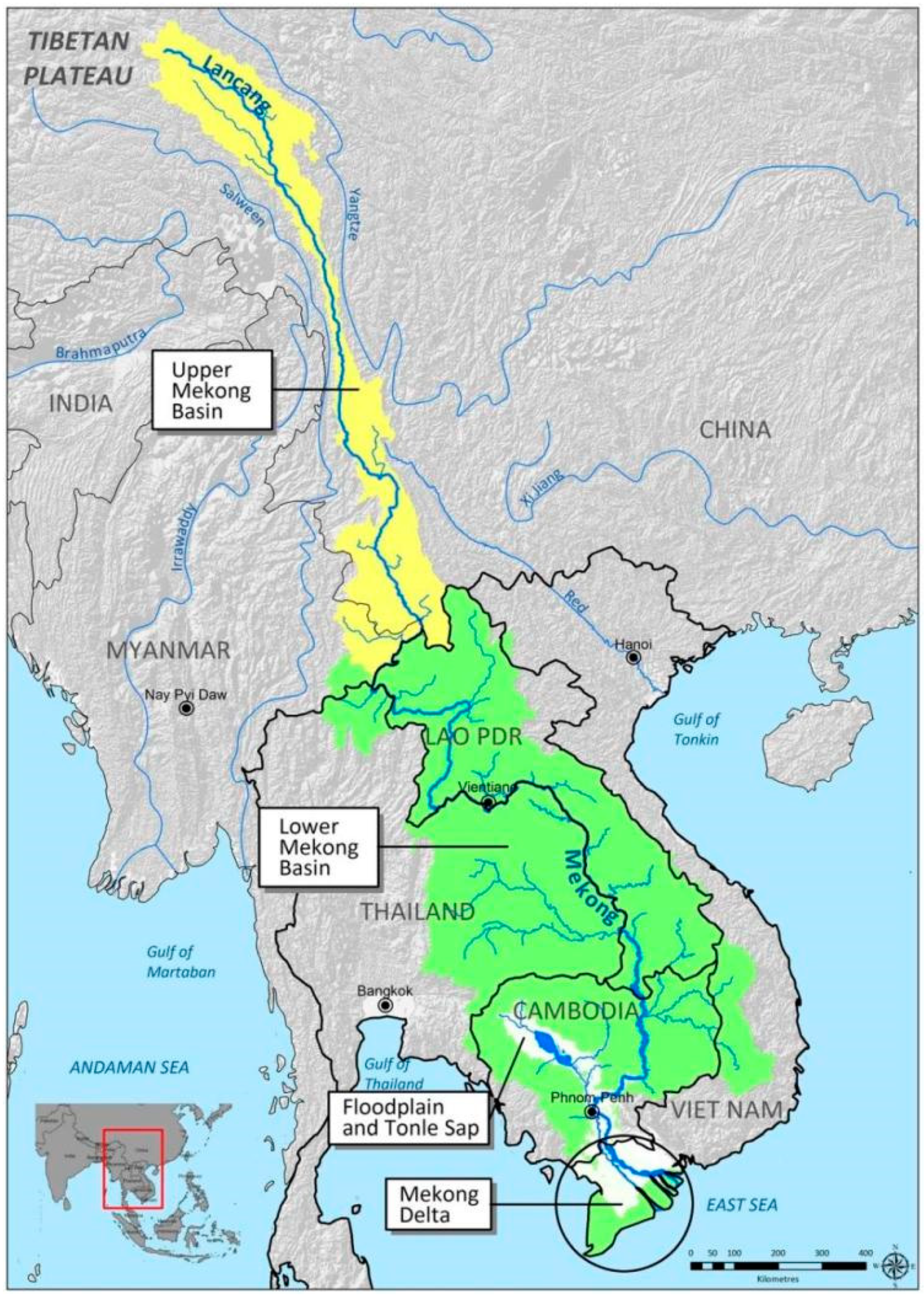
In this study, a bias correction method based on the convolution neural network (CNN) model was developed for the purpose of reanalyzing satellite-derived precipitation data. Additionally, the Mekong River basin has been selected, because it is one of the largest river basins in the world [24]. The Mekong River basin covers six countries (mostly developing countries) with a variety of climates and topographical features. The reliable information on precipitation for the Mekong River basin will be useful in forecasting extreme events such as floods or droughts.

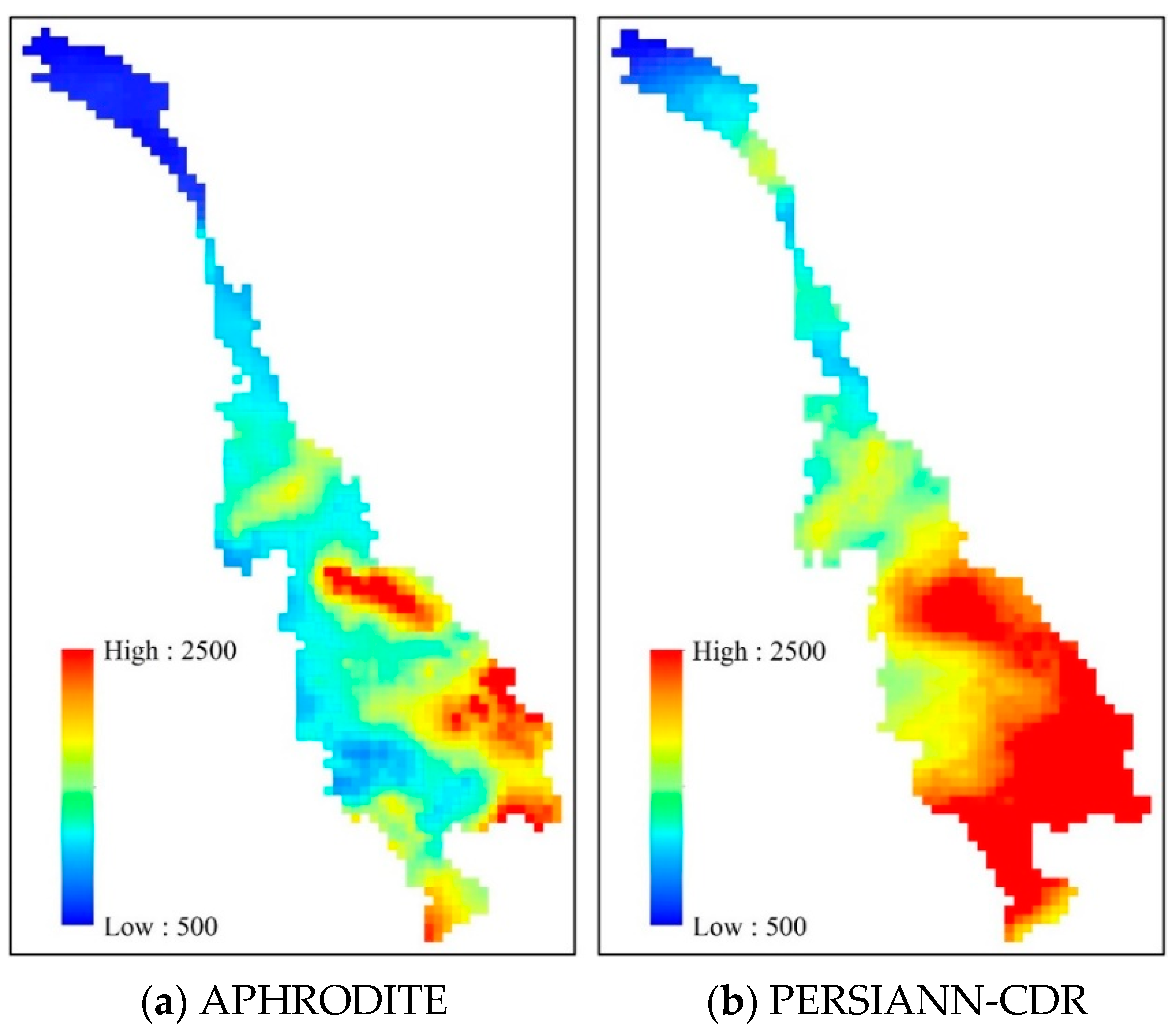
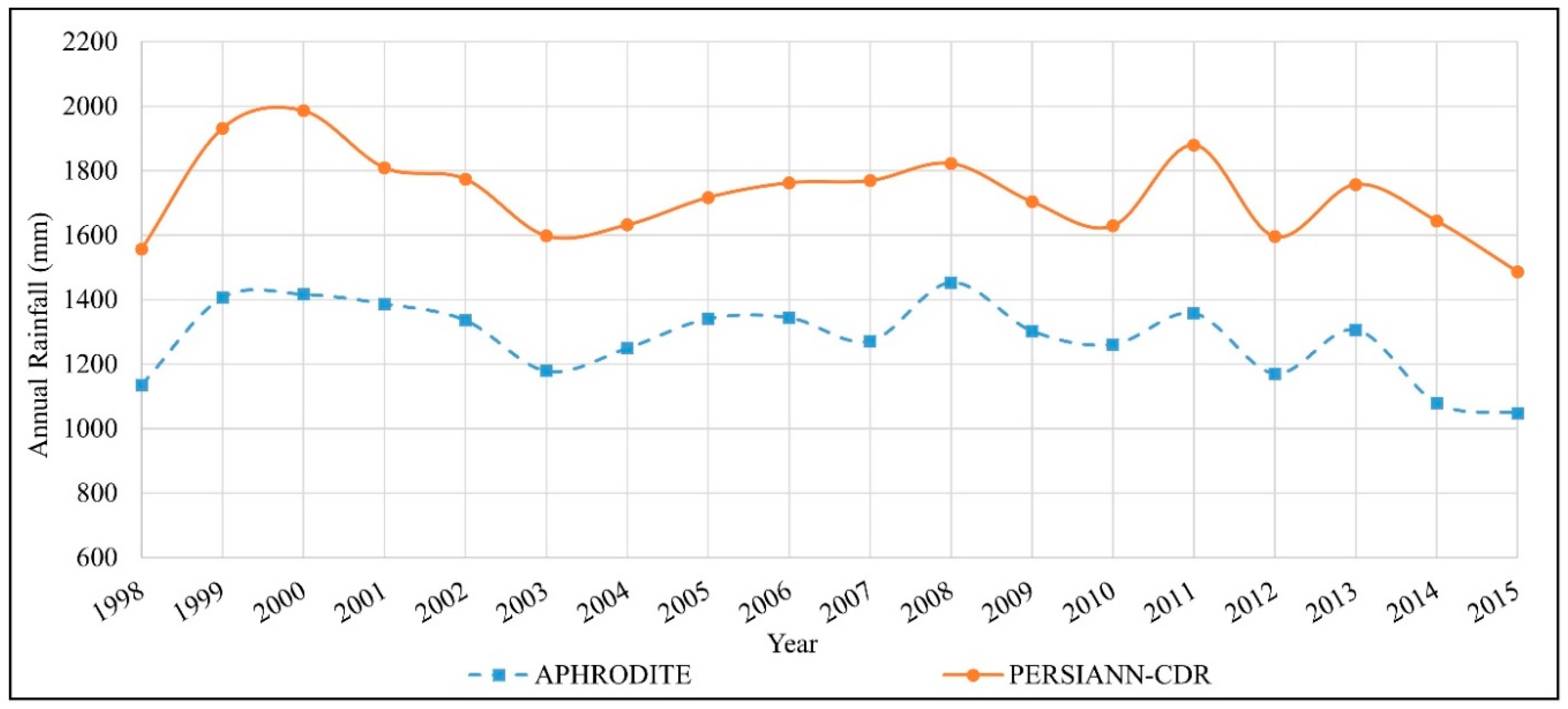
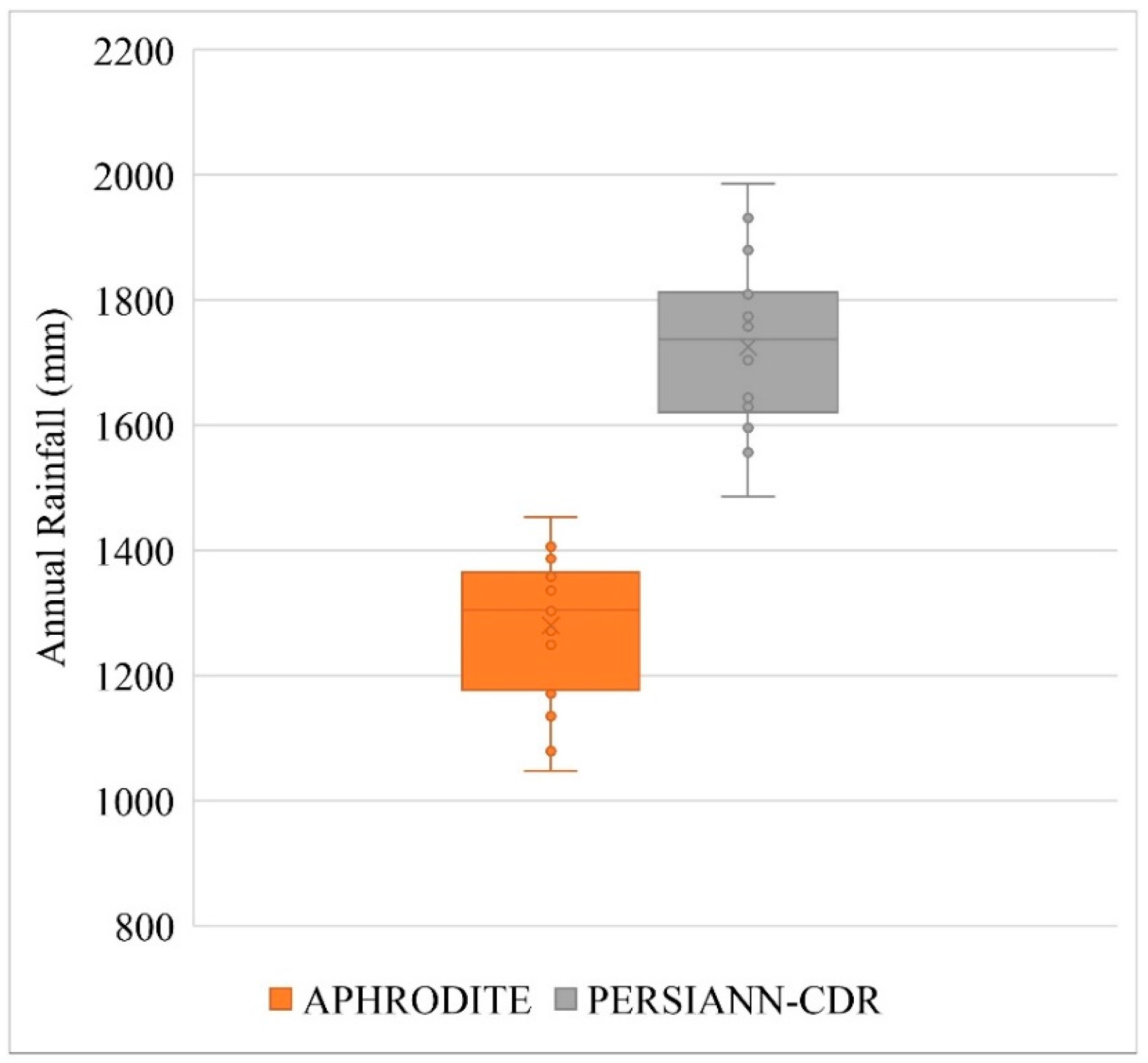
The two gridded precipitation data sources used in this study are the Precipitation Estimation from Remotely Sensed Information using Artificial Neural Networks-Climate Data Record (PERSIANN-CDR) [25] and Asian Precipitation-Highly Resolved Observational Data Integration Towards Evaluation of Water Resources (APHRODITE) [26]. PERSIANN-CDR is a product of the PERSIANN family products, which is useful for research on a scale suitable for extreme weather events [25]. Moreover, PERSIANN-CDR products are available and could be easily accessed for various purposes [8]. Meanwhile, APHRODITE is the gridded precipitation product of an international cooperation program conducted by the Japanese Meteorological Agency and other countries through the collection and analysis from thousands of Asian stations [26]. Therefore, APHRODITE datasets are often considered as observation data for research in the Mekong Region, [27,28,29] as well as for Asia [30,31]. However, a considerable limitation of studies using APHRODITE precipitation data is the availability of this data, which is only available up to 2015 (available 1998-2015 for version V1901), since this is a product conducted through international cooperation projects (APHRODITE projects).

With the aim of producing a more up-to-date dataset than that of the APHRODITE product (which was paused in 2015), sufficiently reliable for the Mekong basin studies, a convolutional autoencoder (ConvAE) neural network model was constructed to correct the rainfall bias from satellite-based products. PERSIANN-CDR is considered a satellite-derived precipitation product, while APHRODITE is referred to as a gauge-based observation product, and both of these products have the same spatial resolution of 0.25°. In addition to the ConvAE neural network model, another bias correction method based on the standard deviation statistic was also applied to correct the pixel-to-pixel bias for the satellite-based products. The performance from these two methods has been examined by comparing statistical properties—for example: mean, standard deviation, distribution, and correlation with an independent observation dataset.

2. Data and Methodology

2.1. Data and Study Area

2.1.1. PERSIANN–CDR Product

PERSIANN-CDR (Precipitation Estimation from Remotely Sensed Information using Artificial Neural Networks-Climate Data Record) is a gridded satelliteFigure precipitation data product among the PERSIANN family products and was developed by researchers at the Center for Hydrometeorology and Remote Sensing (CHRS) at the University of California, Irvine, CA, USA [8]. PERSIANN-CDR precipitation data are generated based on the PERSIANN algorithm using infrared brightness temperature data from Gridded Satellite (GridSat)-B1 as the input and then corrected by the monthly products from the Global Rainfall Climate Project (GPCP) [25]. PERSIANN-CDR provides daily precipitation products with a spatial resolution of 0.25° × 0.25° and a spatial coverage of 60° S–60° N latitude from 1983 to the present time, with a delay of three months [8]. PERSIANN-CDR data are available at http://chrsdata.eng.uci.edu/.

2.1.2. APHRODITE Product

APHRODITE (Asian Precipitation-Highly Resolved Observational Data Integration towards Evaluation of Water Resources) is a project conducted by the Research Institute for Humanity and Nature (RIHN) and the Meteorological Research Institute of Japan Meteorological Agency (MRI/JMA). It generates daily gridded precipitation products by collecting and analyzing rain gauge observation data from thousands of stations throughout Asia. In addition, rainfall data from gauge stations are provided by national meteorological agencies of other countries and undergo quality control before construction of the APHRODITE dataset [32]. The number of rain gauge stations used ranges from 5000 to 12,000, including data on the daily and monthly rain [26]. The key algorithm in building a dataset is the interpolation algorithm from data points to grid cells with sizes of 0.05° using the weighted average method of Spheremap [33]. These data are then corrected utilizing other data sources and grouped into grid cells with sizes of 0.25° or 0.5°, according to the weighted average method by area. In this study, the APHRODITE precipitation data product version V1901 (MA), available from 1998 to 2015, was exploited with a daily temporal resolution and a spatial resolution of 0.25°. The APHRODITE products are available at http://aphrodite.st.hirosaki-u.ac.jp/.

2.1.3. Study Area

The Mekong River is one of the largest river systems in the world, with a length of approximately 4763 km [24]. Originating from the Himalayas (China), it flows through Myanmar, Thailand, Laos, Cambodia, and Vietnam before flowing into the East Sea. The Mekong River has an abundant flow with a mean annual discharge of approximately 446 km³, and its basin covers a large area of 810,000 km² [24]. The Mekong River basin is often divided into upper and lower basins. The Upper Mekong Basin (UMB) is located in China, where it is known as the Lancang River. Upstream flows account for only a small portion of the total annual flow of the Mekong River at approx. 15–20% [34]. The Lower Mekong Basin (LMB) starts at the border between China and Lao PDR and stretches into the East Sea. Based on 2015 estimates, there are approximately 65 million people living within the LMB [24]. The location of the Mekong River basin is shown in Figure 1.

One of the important features of the Mekong River basin is the diversity of the climate it experiences, which ranges from temperate to tropical. Thus, the distribution of precipitation in the catchment is also uneven both spatially and temporally due to the topographic characteristics. The natural hydrological regime of the Mekong River has a large difference in the dry season flow (from December to May) and the wet season (from June to November) caused by the southwest monsoon. The annual flood season in the Mekong River usually lasts for four months, from July to October. The flow during this period accounts for 80–90% of the total annual flow [35] and plays an important role in the LMB. As mentioned above, the distribution of the mean annual rainfall over the basin is highly variable. According to a previous report [36], the annual rainfall decreases along the west away from the mountains, with a clear east–west rainfall gradient. The annual rainfall in the UMB ranges from 600 mm in the Tibetan Plateau to 1700 mm in the mountains of Yunnan, China. For the LMB, the annual average rainfall ranges from 1291 mm to 1992 mm per year over the period 1901–2010 [24].

In this study, the Mekong River basin was selected as the case study, and the two rainfall products described above (PERSIANN-CDR and APHRODITE) were used for different purposes. Both of these products are daily gridded precipitation data products with a spatial resolution of 0.25°. While PERSIANN-CDR products are employed as satellite-based precipitation data, APHRODITE products are used as observed precipitation data. Brief information on the two gridded rainfall data is provided in

Table 1. Description of the gridded precipitation datasets used in this study. APHRODITE: Asian Precipitation-Highly Resolved Observational Data Integration towards Evaluation and PERSIANN-CDR: Precipitation Estimation from Remotely Sensed Information using Artificial Neural Networks-Climate Data Record.

Dataset	Version	Spatial/Temporal Resolution	Area Coverage	Time Coverage	Sources
APHRODITE	V1901	0.25°/daily	Monsoon Asia	1998–2015	[26]
PERSIANN	CDR	0.25°/daily	Near-global	1983–present	[25]

.

The daily rainfall data series was collected for 18 years, from 1998 to 2015, due to the APHRODITE projects having been paused in 2015. These data were then processed for the purpose of producing a raster dataset on precipitation for the Mekong basin. The cell size of the raster dataset was 0.25° × 0.25° (referenced to a spatial resolution of 0.25°). For the Mekong River basin, the total number of grid cells in each raster file was 6000, which corresponded to a pixel matrix with 100 rows and 60 columns. Figure 2 illustrates the precipitation spatial distribution over the Mekong River basin in 2000. This was the year of the most severe event in terms of the area inundated in over 70 years, which corresponds to an average recurrence interval of 1:50 years at Kratie Station [34].

Both precipitation products depict the trend of the spatial rainfall distribution driven primarily by topography and precipitation decreases to the west away from the mountains. However, the distribution of rainfall in 2000 over the Mekong basin was highly variable, especially in the LMB. While areas of high precipitation in excess of 2000 mm were found only in the North-Central of Lao PDR and the eastern mountainous region bordering Vietnam in the APHRODITE product (Figure 2a), the PERSIANN-CDR product indicated that high precipitation was found in most of the areas over the LMB (Figure 2b). In addition, summary of the mean annual precipitation of the Mekong River basin during the 18-year study period is illustrated in Figure 3 and Figure 4.

During the study period (18 years), both gridded precipitation products presented a high correlation of the mean annual precipitation. Figure 3 and Figure 4 also demonstrate the overestimation trend of PERSIANN-CDR precipitation data when compared to APHRODITE precipitation data. In addition, there existed considerable gaps between the satellite-derived precipitation data (PERSIANN-CDR) and observed data (APHRODITE) due to the dependence of precipitation on the spatiotemporal distribution, as well as the specific characteristics of the area. The biggest gap in annual precipitation between the two products was recorded in 2000 to be approx. 570 mm. This study presents an efficient approach based on a CNN model to reanalyze satellite-based precipitation data for the Mekong River basin.

2.2. Methodology

2.2.1. Convolutional Neural Network

A convolutional neural network (CNN or ConvNet) is a class of deep neural networks that have proven very effective in contexts of computer vision, such as image recognition, classification, or identifying objects. Similar to ordinary neural networks, CNNs are made up of neurons that have learnable weights and biases. However, CNN architecture is designed with a clear assumption that inputs are the 2D structure of an input image. This allows CNN to encode certain properties into their architecture and then perform a more efficient forwarding function and significantly reduce the number of parameters in the network compared to conventional neural networks [37]. In addition, a CNN has a grid topology for processing data, which enables them to be more efficient when working with spatial data.

The structure of a CNN model is usually a combination of three kinds of layers: the convolution layer, the pooling layer, and the fully connected layer (this layer may not be needed for some problems). These layers are often arranged in a chain for a simple CNN model, either stacked or combined with other architectures to construct complex CNN models. Depending on the different problems, the number of layers and the order of the layers may vary. With respect to the gridded precipitation bias correction problem, a deep-learning neural network model has been proposed based on a combination of a convolutional neural network and autoencoder architecture, called the convolutional autoencoder (ConvAE) neural network.

Autoencoders comprise a type of artificial neural network that belongs to the unsupervised learning category in terms of deep-learning classification. The autoencoder is designed with the purpose of copying its input data to its output [38]. The network architecture of an autoencoder usually consists of two parts: the encoder and the decoder. An encoder employs the process of learning how to compress and encode data effectively by reducing the data dimension and by passing the noise. A decoder involves the process of reconstructing the encoded data above into a representation that is as close to the input data as possible. A typical architecture of an autoencoder is illustrated in Figure 5.

The ConvAE neural network model was constructed in this study for the purpose of adjusting the bias of the satellite-derived precipitation products (PERSIANN-CDR) for the Mekong River basin. The observed data used for comparison with the corrected data from PERSIANN-CDR precipitation is the APHRODITE precipitation. Both products are daily gridded precipitation data with a spatial resolution of 0.25° and have been described in detail in Section 2.1 (Data and Study Area).

2.2.2. Statistical Method

In addition to the ConvAE neural network model, a statistical-based approach (the standard deviation method) was also applied to reanalyze the PERSIANN-CDR precipitation data. The main purpose of this method is to adjust satellite-based data such that corrected data has similar statistical properties (for example: mean, standard deviation, probability distribution, or correlation matrices) as the measured data in the same period. The correction of the spatiotemporal precipitation bias between the two gridded products, from satellite-derived data to observed data, is carried out by pairing each of the grid cell value pairs corresponding to the two products in the Mekong River basin for comparison. Therefore, a modified formula based on the standard deviation method is proposed to adjust the satellite-based precipitation according to both the average observed data and observed variance (refer to Immerzeel [40] and Bouwer et al. [41]), as follows:

$${a^{\prime }}_{sat}=\left(\frac{a_{sat}-{\overline{a}}_{sat,j}}{{\sigma }_{sat,j}}\right).{\sigma }_{obs,j}+{\overline{a}}_{obs,j}$$

(1)

where ${a^{\prime }}_{sat}$ is the corrected precipitation data from the satellite-based precipitation data, $a_{sat}$ the uncorrected precipitation data (or satellite-based data), ${\overline{a}}_{sat,j}$ the average of the satellite-based precipitation data corresponding month jth (January–December) over the study period, ${\sigma }_{sat,j}$ the standard deviation of the satellite-based precipitation data corresponding month jth over the study period, ${\sigma }_{obs,j}$ the standard deviation of the observed precipitation data corresponding month jth over the study period, and ${\overline{a}}_{obs,j}$ the average of the observed precipitation data corresponding month jth over the study period. All variables described in Equation (1) are basic information corresponding to a grid cell in the Mekong River basin.

2.2.3. Performance Metric Index

In order to evaluate the performance of the gridded precipitation bias correction methods, several statistical indicators were applied to measure the difference between the corrected and observed data by comparing the average pixel-by-pixel difference. Let (x₁, y₁) and (x₂, y₂),…, (x_n, y_n) be n pairs of values from two different datasets. These parameters are calculated as follows:

$$NSE=1-\frac{{\displaystyle \sum _{i=1}^n{\left(x_i-y_i\right)}^2}}{{\displaystyle \sum _{i=1}^n{\left(x_i-\overline{x}\right)}^2}}$$

(2)

$$RMSE=\sqrt{\frac{1}{n}{\displaystyle \sum _{i=1}^n{\left(x_i-y_i\right)}^2}}$$

(3)

$$MAD=\frac{1}{n}{\displaystyle \sum _{i=1}^n\left|x_i-y_i\right|}$$

(4)

$$Bias=\frac{1}{n}{\displaystyle \sum _{i=1}^n\left(x_i-y_i\right)}=\overline{x}-\overline{y}$$

(5)

where NSE means the Nash–Sutcliffe efficiency, RMSE means the root mean square error, MAD means the mean absolute difference, and $\overline{x}$ and $\overline{y}$ are the mean values of the two data sources, respectively.

In addition to the aforementioned indicators, the covariance (Cov) and correlation (Corr) are also important indicators when evaluating the spatial and temporal fluctuations of two data sources.

$$Cov=\frac{1}{n}{\displaystyle \sum _{i=1}^n\left(x_i-\overline{x}\right)}\left(y_i-\overline{y}\right)$$

(6)

$$Corr=\frac{Cov}{{\sigma }_x{\sigma }_y}$$

(7)

with ${\sigma }_x$ and ${\sigma }_y$ denoting the standard deviations of x and y.

3. Model Application

This study has proposed two approaches, (1) based on the ConvAE model, and (2) the statistical method, to reanalyze the satellite-derived precipitation. Besides, the results of this study are closely related to open-source software libraries. Accordingly, the programming language used throughout the study was Python [42]. Several processes such as data processing, data management, or data visualization were accomplished using Numpy [43], Pandas [44], and Matplotlib [45] libraries. For the ConvAE model, our work exploited a Python deep-learning library, Keras—A high-level neural network API (application programming interface) [46]—and used TensorFlow [47] as the backend. All ConvAE models were implemented on Google Colaboratory (also known as Colab), which is a free Google cloud service based on the Jupyter Notebook [48].

3.1. ConvAE Neural Network

For the ConvAE network model, the input data (PERSIANN-CDR) and target data (APHRODITE) were two daily gridded precipitation products and have the same grid size of 100 × 60, as stated above. Similar to other neural network models, the performance of the ConvAE model undergoes careful evaluation through training, validation, and testing. All of the 18-year data available were divided into three nonoverlapping datasets for these three purposes. The first dataset employed for the purpose of training the model covered 14 years (1998–2011). The second dataset, spanning 2 years (2011–2013), was used for the purpose of validating the model performance. The remaining dataset, spanning the period 2014–2015 (2 years), was used to objectively verify the performance of the model through comparison with two corrected datasets from the ConvAE neural network model and standard deviation method.

For most CNN models, there is no specific reference structure for the selection of layers, number of layers, and order of layers, as well as the hyperparameters inside the model. Proposing an optimal architecture is usually based on a careful trial and error evaluation process. With respect to the precipitation bias correction problem from satellite-based products, several ConvAE models developed based on typical structures, such as VGGNet [49] or Unet [50], were also considered. However, the corrected data from these models were not satisfactory when compared to the observed data.

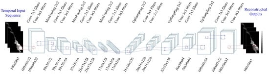
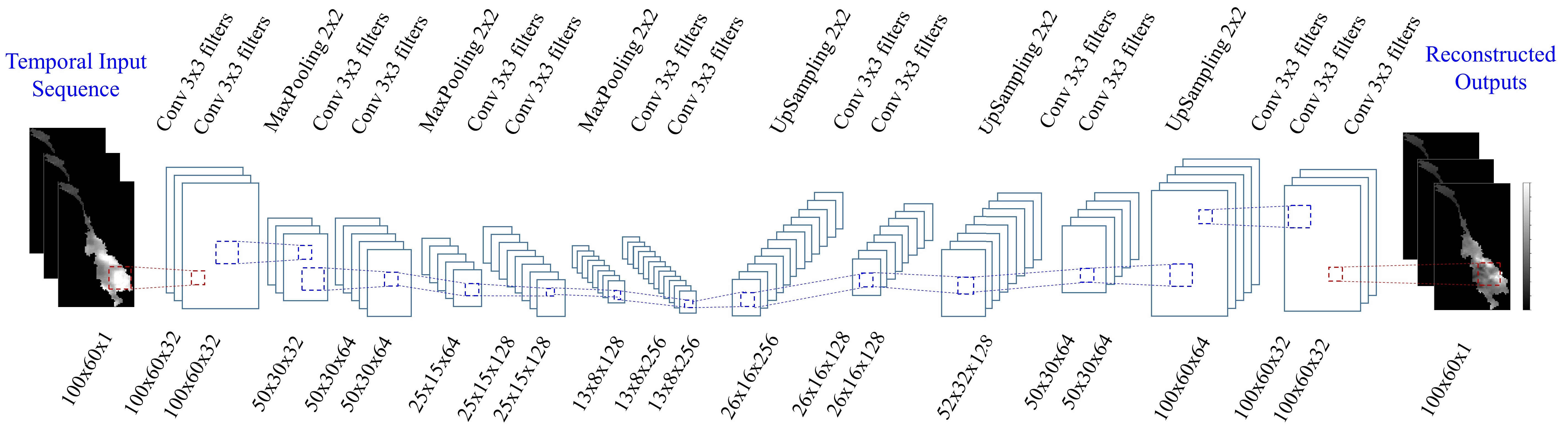
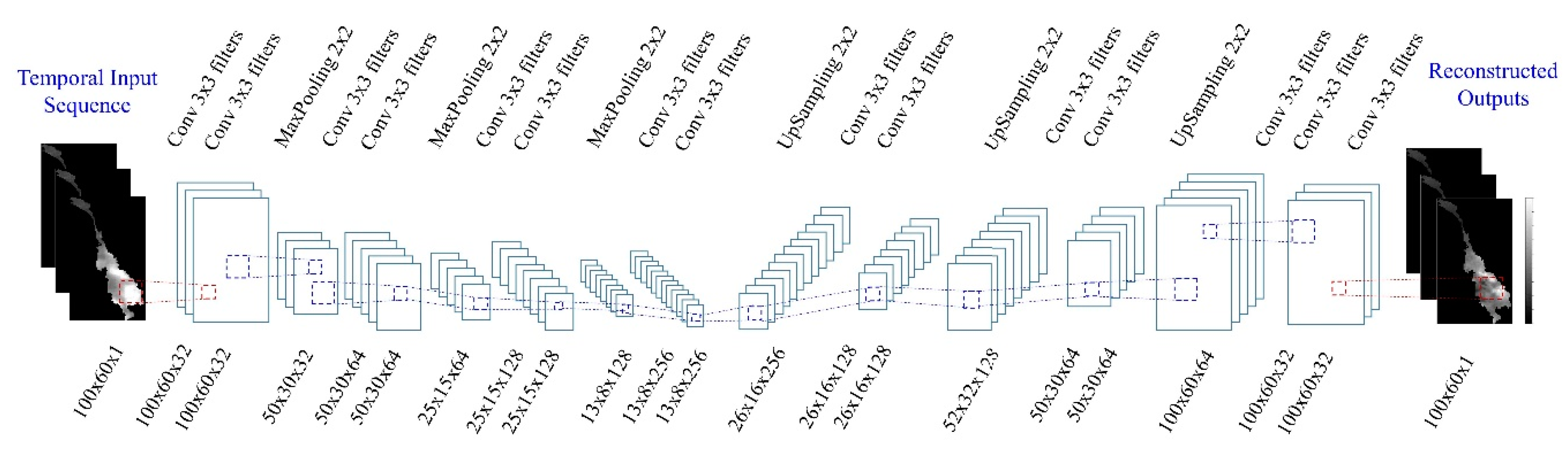
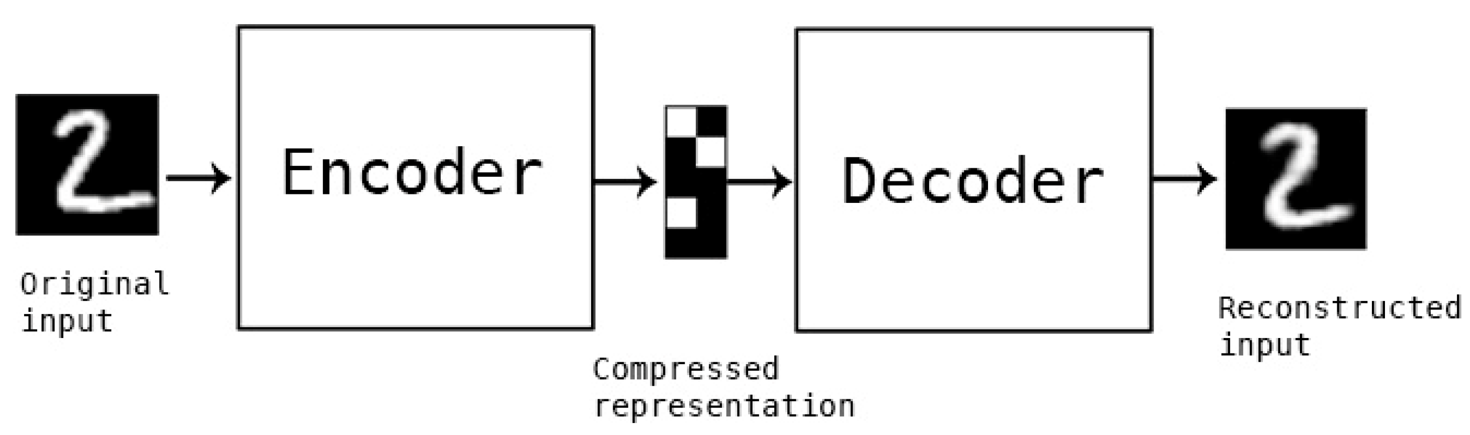
According to Karpathy [37], the most prevalent form of CNN architecture is stacking several convolution layers, followed by pooling layers, and repeating this pattern until the desired spatial dimension is reached. In this study, the proposed ConvAE model has the structure illustrated in Figure 6, which is a combination of two network architectures, the encoder network, and the decoder network.

The model’s input and target data are raster data (2-dimensional) and have the same dimensions of 100 × 60 × 1, where the parameters correspond to the height, width, and depth in the CNN model [37], respectively. In the first part, the encoder architecture, the arrangement of two convolution layers is stacked before every pooling layer, with the idea of making the network model larger and deeper to better capture the complex features of the input data [37].

For the convolution layer, the filter parameter is referred to as the number of output filters in convolution required to generate feature maps by applying convolution operations. The recommended number of filters in this study started at 32 and then increased to 64, 128, and 256 in the deeper layer. The selection of the number of filters has a power function of 2, with the aim to save computer resources when processing data. In addition to the number of filters, the kernel size parameter is also an important parameter in the convolution layer, specifying the width and height of the 2D convolution window [46]. According to Rosebrock [51], the kernel size values are usually odd numbers, and large kernel values (5 × 5 or 7 × 7) are often considered to be applied to data larger than 128 × 128 in order to quickly reduce the spatial dimensions. For this study, the recommended kernel size value in the convolution layers is 3 × 3, because the spatial dimension of the input data is only 100 × 60.

Adding a pooling layer after the convolution layer is a popular pattern used for arranging layers within the CNN. The pooling operation is applied on each feature map (which is created after the convolution operation) using the pool size parameters to produce a new set with the same number of feature maps; however, the dimension of each feature map will be reduced. The size of the pooling operation (pool size) is smaller than the size of the feature map, and a pool size value of 2 × 2 pixels is usually applied to each pooling operation [52]. This means the spatial dimension of the feature map will be halved (both horizontal and vertical) after the pooling operation. Moreover, AveragePooling and MaxPooling are two widely used functions to reduce the spatial dimension of a feature map. While AveragePooling calculates the average value for a patch on a feature map, the MaxPooling chooses the maximum value. Before deciding MaxPooling was the pooling function in this study, a comparison of the model performance was carried out by applying the two mentioned above functions in turn. The results indicated that the MaxPooling function is better at capturing higher values than the AveragePooling function.

In the decoder part, reconstructing the encoded data is implemented using a combination of each UpSampling layer with two stacked convolution layers and repeating until the desired format is reached. The UpSampling layer is simply understood as a way of scaling up of the data using the nearest neighbor algorithm or bilinear interpolation. Here, a size parameter of (2, 2) inside the UpSampling layer has been selected to simply double the dimensions of the input. In accordance with each UpSampling layer, the number of filters in the convolution layers decreases from 256 to 128, 62, and, finally, 32 after reaching the desired size of 100 × 60. At the last convolution layer, the number of filters was set to 1 so that the reconstructed data had the same output size as the input size.

In addition to the construction of the ConvAE model structure, one of the important issues for deep-learning neural network problems is the selection of hyperparameters, such as loss function, optimization algorithm, or the number of epochs for the training process. The recommended parameters in this study have undergone careful evaluation and comparison of performance. The proposed loss function is the mean square error (MSE), which has shown superior performance compared to other loss functions, such as the mean absolute error. Along with the loss function, the Adam optimization algorithm [53] was considered suitable for this study; it is widely applied in studies of deep-learning applications. Additionally, the ConvAE model has been established to record the necessary information during the training and validation processes. Besides, the recommended number of epochs in the ConvAE model was 5000, with a batch size of 32. Finally, in order for the ConvAE model to be effectively adjusted, the early stopping technique was applied to prevent overfitting problems (if possible) [54], and the model checkpoint technique was developed to save the model performance information before the model stopped.

3.2. Standard Deviation Method

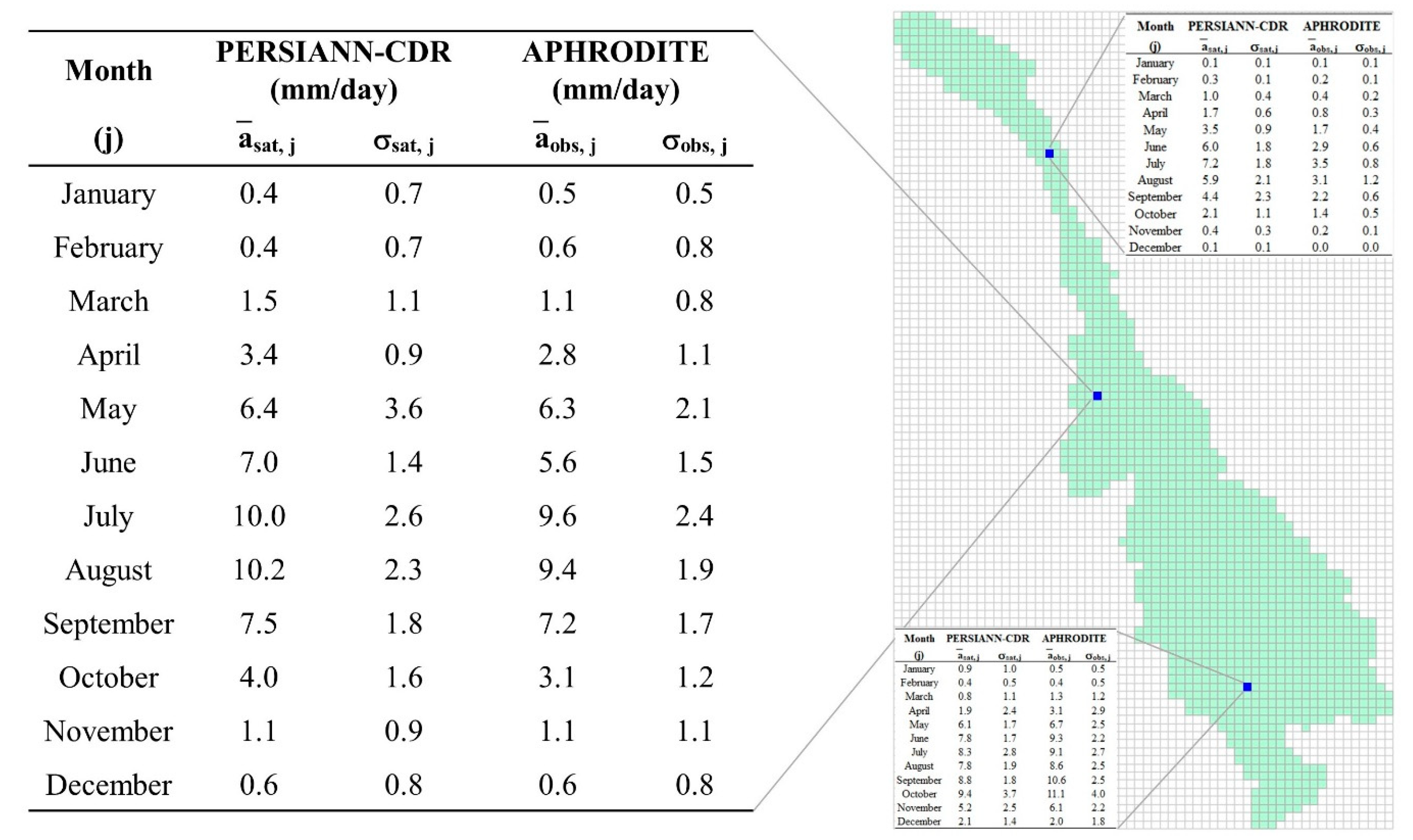
For the standard deviation method, data were corrected from PERSIANN-CDR products based on Equation (1). All available data for 18 years were divided into two independent datasets. The statistical dataset for 1998 to 2013 (16-year baseline period) was used to calculate the statistical indicators mentioned in Equation (1) of the PERSIANN-CDR and APHRODITE precipitation products. The remaining 2-year dataset (2014–2015) was employed to examine the performance of the statistical method and compare it with the corrected data acquired from the ConvAE model.

Both of the gridded precipitation products had the same dimensions of 100 × 60 after processing, with the total number of cells being 6000. Due to the fact that this study was conducted in the Mekong River basin, 1112 grid cells were counted in the catchment, and other cells outside the catchment were ignored. From the data for a 16-year baseline period, statistical properties such as the mean and the standard deviation corresponding to each month of the two products were calculated. Note that each grid cell has different statistical properties. The basic statistical properties of a grid cell in the Mekong basin are illustrated in Figure 7.

The two-year independent dataset (2014–2015) was used to evaluate the method performance through the cell-by-cell pairing of the corrected data and observed data, for which the corrected data were calculated using Equation (1) from the PERSIANN-CDR product.

4. Results and Discussion

In this section, an independent dataset (testing dataset) spanning two years (2014–2015) was adopted to evaluate the performance of two methods of correcting the daily precipitation bias from satellite-based products. First, the PERSIANN-CDR data were employed as the input for the models to generate two corrected datasets, which correspond to the two methods mentioned above. Then, these corrected data were used to evaluate the performance of the two methods by comparison with the gauge-based data (APHRODITE).

As for the ConvAE neural network model, before verification using a testing dataset was performed, the model underwent the training and validation process, as described in Section 3.1. Conducting a validation step is necessary to select the optimal parameters of the model and to prevent overfitting problems often faced when working with neural networks. In this study, we skipped presenting the results of the validation step. Instead, the optimal parameters of the model obtained from the validation step were used to conduct the testing step.

4.1. Temporal Correlation

The performance metric indicators used to evaluate the temporal correlation between the observed and corrected precipitation products over the Mekong River basin during the testing period are the MAD, RMSE, and NSE. The comparison results are depicted in

Table 2. Total annual precipitation over the Mekong basin during the testing period. ConvAE: convolutional autoencoder.

Process	Year	Observed (mm/Year)	Corrected by ConvAE (mm/Year)	Corrected by Statistic (mm/Year)	Satellite-Based (mm/Year)
Testing	2014	1086	1125	1025	1661
	2015	1050	1095	823	1498
Average rainfall (mm/year)		1068	1110	924	1579

and

Table 3. Temporal correlation of the monthly total precipitation between the corrected products and observed data during the testing period. MAD: mean absolute difference, RMSE: root mean square error, and NSE: Nash–Sutcliffe efficiency.

Compared with Observed	Testing Period (Month)	MAD (mm/Month)	RMSE (mm/Month)	NSE
ConvAE	24	12.6	19.1	0.97
Statistic	24	22.3	38.4	0.83
Satellite	24	43.1	54.1	0.61

, and Figure 8 and Figure 9.

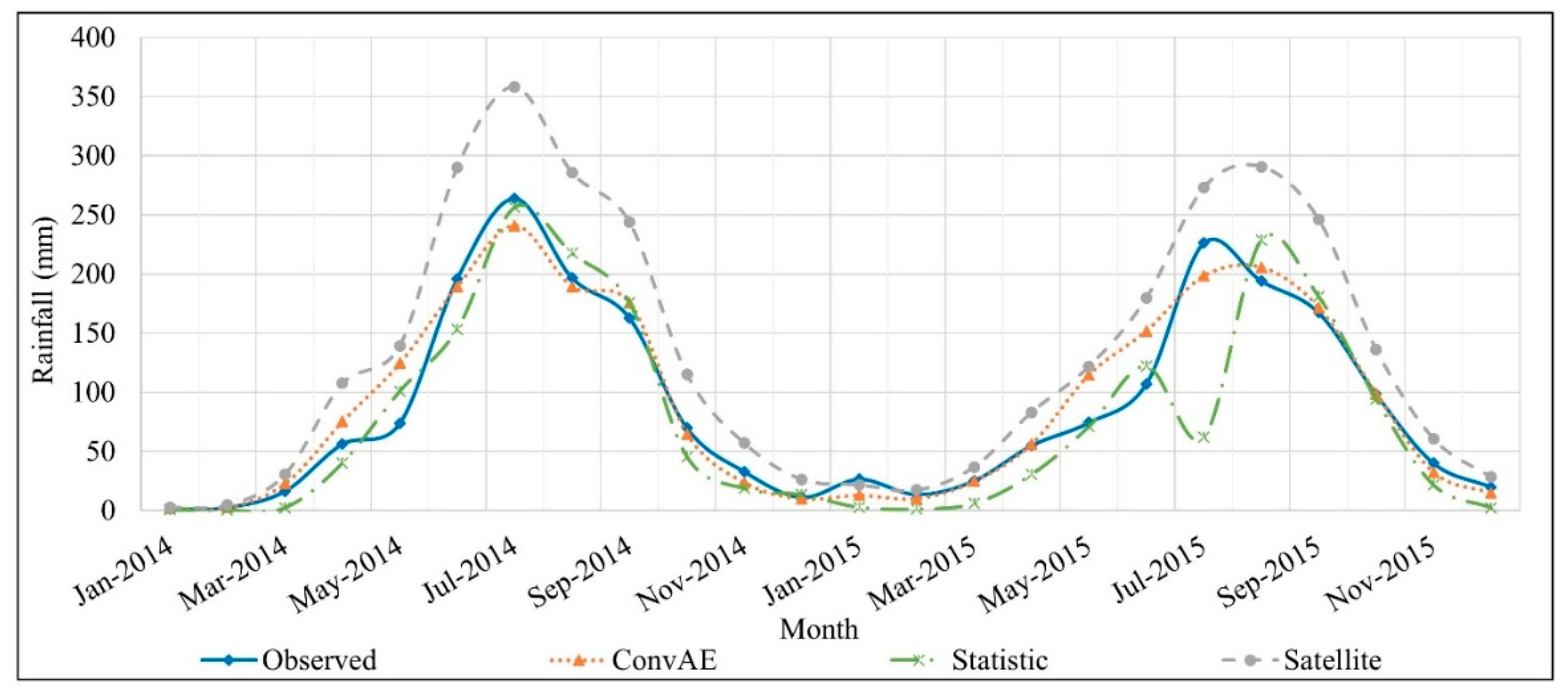
Table 2 provides information on the mean annual precipitation over the Mekong basin corresponding to the rainfall products during the two-year testing period from January 2014 to December 2015. Overall, the satellite-based precipitation shows a tendency to be overestimated compared to the observed data. Over the Mekong River basin, the average annual rainfall based on the observed data (APHRODITE) was only 1068 mm, an amount smaller by about 500 mm than the corresponding amount given by the satellite-based data (PERSIANN-CDR). For the two corrected precipitation products, the ConvAE model exhibits better performance with the standard deviation method; the values of the average annual rainfall for these two products are 1110 mm and 924 mm, respectively.

An opposite trend was witnessed more clearly when the total monthly precipitation obtained from the products was of interest (see Table 3 and Figure 8). Comparing correlations between the corrected data series and observed data, the ConvAE model illustrated superior performance compared to the statistical method, with an NSE value of 0.97 and a MAD value of 12.6 mm. The values corresponding to the two indices, NSE and MAD, for the statistical methods were modest at 0.83 and 22.3 mm, respectively. Additionally, Figure 8 also indicates the uncertainty of the standard deviation method, as the total amount of rainfall adjusted in July 2015 was abnormal compared to that in the remaining months. One of the reasonable causes of the irregularity in the total corrected precipitation could be the satellite-based data.

4.2. Probability Distribution

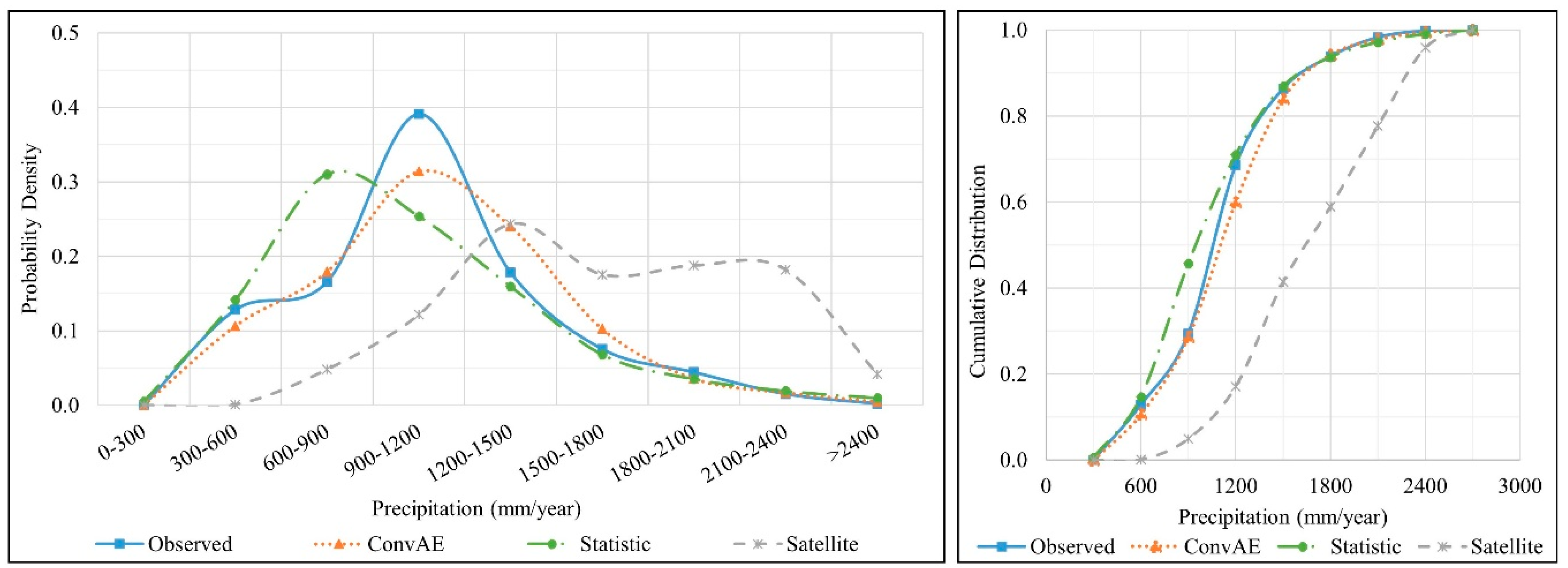
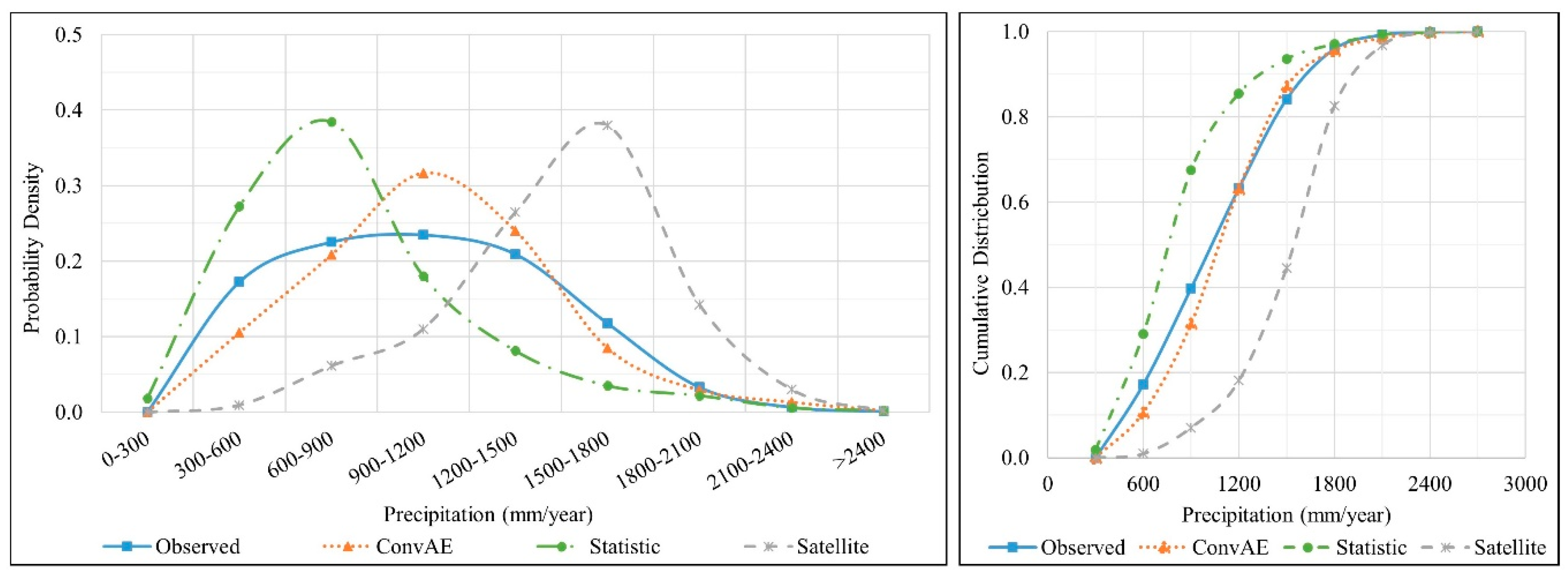
In addition to comparing the mean annual precipitation correlation of the products over the Mekong River basin, the probability distribution of the rainfall data by grid cell was also considered. The probability density function (PDF) and cumulative distribution function (CDF) are two statistical functions utilized to describe the probability distribution of the total precipitation by grid cells. The probability distribution of the total rainfall in the two-year testing period (2014–2015) is shown in Figure 9 and Figure 10.

As can be seen in Figure 9 and Figure 10, corrected precipitation data from satellite-based products demonstrate a certain similarity to observed data. For the statistical method, the two-year corrected data reveals that this model continues to exhibit uncertainty, which is more evident in the PDF curves of both 2014 and 2015. By contrast, the ConvAE model continues to illustrate a stable performance not only through the PDF curve but, also, through the CDF curve. With respect to the observed data, the annual precipitation measured in the Mekong River basin was concentrated in the range of 900 mm to 1200 mm, which accounted for nearly 40% in 2014 and approximately 25% in 2015. In contrast to the observed rainfall products, the satellite-based rainfall product illustrated significant differences in both the probability distribution and precipitation intensity. Specifically, the total rainfall measured in 2014 mainly ranged from 1200 mm to 2400 mm (accounting for approximately 79%) and ranged from 1200 mm to 2100 mm (about 78%) in 2015.

As for the two corrected rainfall products, Figure 9 and Figure 10 also reveal that the ConvAE model outperforms the statistical method. Although the statistical method achieves notable performance when evaluating the temporal correlation with the NSE value of 0.83 and the RMSE value of 38.4 mm (Table 3), the probability distribution of this precipitation product shows a low correlation with the observed precipitation. In addition, the adjusted rainfall from the statistical method was mainly in the range of 600 mm to 900 mm for the two-year testing period, accounting for well above 31% for 2014 and nearly 38% for 2015.

In the case of the ConvAE model, the corrected data indicated better agreement with the observed data in terms of the PDF and CDF. The total annual precipitation recorded in the Mekong basin from the ConvAE model had the same probability distribution pattern with the observed data in both years of testing. Moreover, this value chiefly ranged from 900 mm to 1200 mm and accounted for the similarity percentage for both years at about 31%.

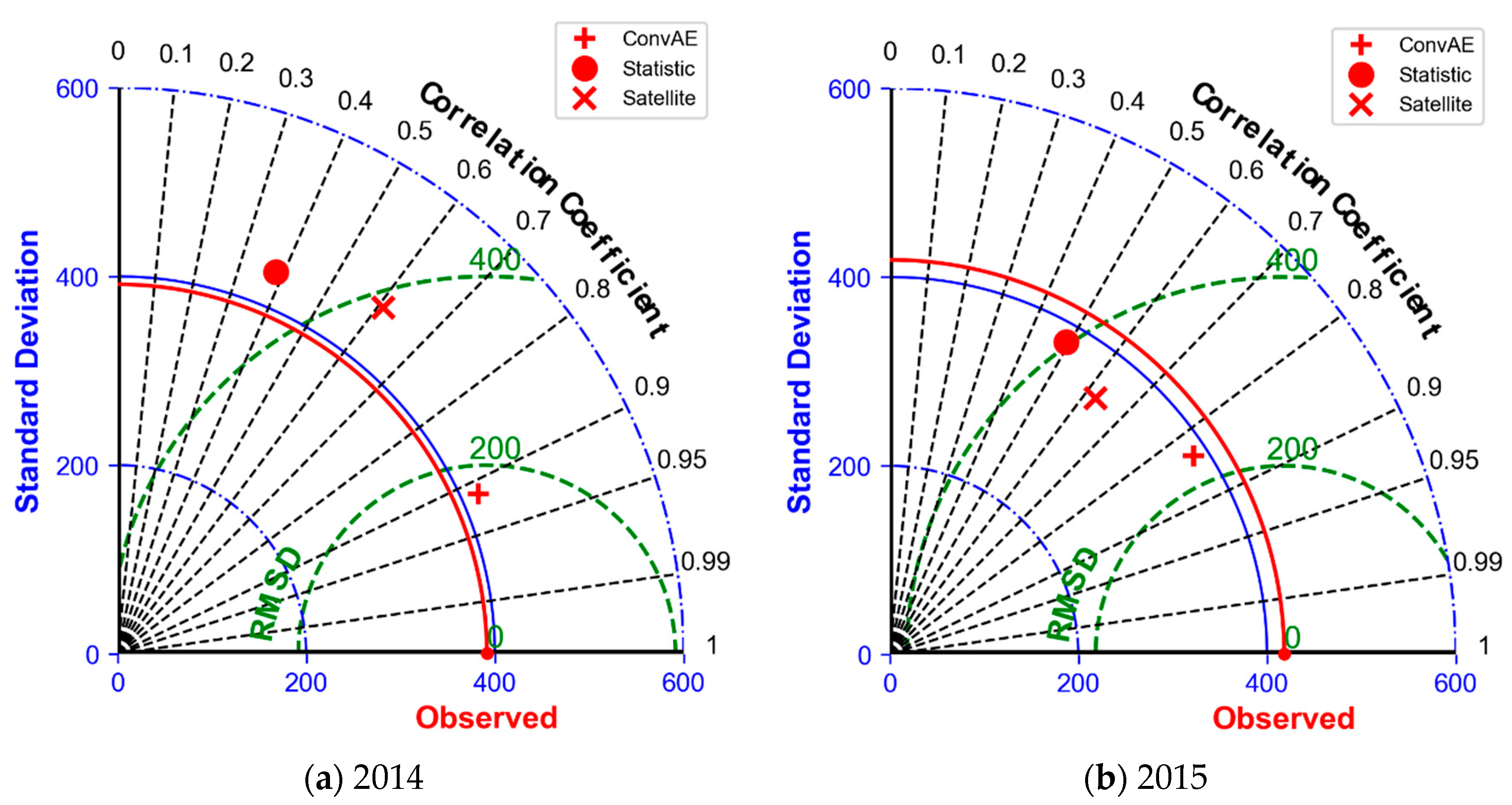
In addition, another statistical comparison was also conducted to evaluate the correlation of the annual precipitation per grid cell between the rainfall products. These statistical criteria are presented in the Taylor diagram (Figure 11).

In the Taylor diagrams [55,56], these datasets represent the total annual rainfall of each grid cell across the Mekong basin, corresponding to the precipitation products based on the observed, ConvAE, statistic, and satellite, respectively. It can be seen that the ConvAE model generally outperforms other products, with higher correlation coefficients (about 0.91 for 2014 and 0.84 for 2015) and lower in terms of the RMSD and standard deviations in both years of the testing period. For 2014, the ConvAE model agrees well with the observations, with a standard deviation of 410 mm/year compared to the observed value of 390 mm/year. Meanwhile, the statistical model illustrates poorer performance than the satellite-based product when the evaluation criteria such as the correlation coefficients and RMSD are significantly lower (see Figure 11a).

In the case of 2015 (Figure 11b), the Taylor diagram recorded a similar trend as in 2014, where the ConvAE model performed the best performance, while the statistical model depicted uncertainty. The poor performance of the statistical method results from all the statistical values represented in the Taylor diagram, including a correlation coefficient of 0.50, an RMSD value of 400 mm/year, and a standard deviation of 390 mm year. The satellite-based data have a moderate correlation coefficient (only 0.62 compared to 0.84 of the ConvAE model); however, there is less spatial variation than the other two models (with a standard deviation of 350 mm/year compared to the observed value of 420 mm/year).

An overview of the comparison of the temporal correlation and probability distribution has revealed an instability and uncertainty of the statistical method in adjusting the rainfall products in the Mekong River basin. Although the mean annual rainfall across the basin in the two-year testing was 924 mm/year, which is close to the observed value of 1068 mm/year (see Table 2 and Table 3), the annual rainfall per grid cell exhibited an opposite trend (see Figure 11). On the other hand, a stable high performance was noted in the case of the ConvAE model in both comparisons conducted above.

4.3. Spatial Correlation

In addition to taking into account the temporal correlation, a comparison of the spatial correlation between the corrected precipitation data and observed data was also conducted to evaluate the effectiveness of the two bias corrective methods. The spatial correlation between the precipitation products was assessed by comparing the average pixel-by-pixel differences (by RMSE, MAD, and bias values) and correlation index (Corr). The spatial distribution pattern of the precipitation products is illustrated in Figure 12, Figure 13 and Figure 14. The comparative results in the two-year testing dataset are summarized in

Table 4. Spatial correlation of the annual precipitation between the corrected products and observed data during the testing period.

Compared with Observed	2014			2015
	ConvAE	Statistic	Satellite	ConvAE	Statistic	Satellite
RMSE (mm/year)	174	467	690	236	463	561
MAD (mm/year)	134	355	582	187	368	481
Bias (mm/year)	39	−61	574	46	−226	448
Correlation	0.91	0.32	0.61	0.84	0.46	0.63

.

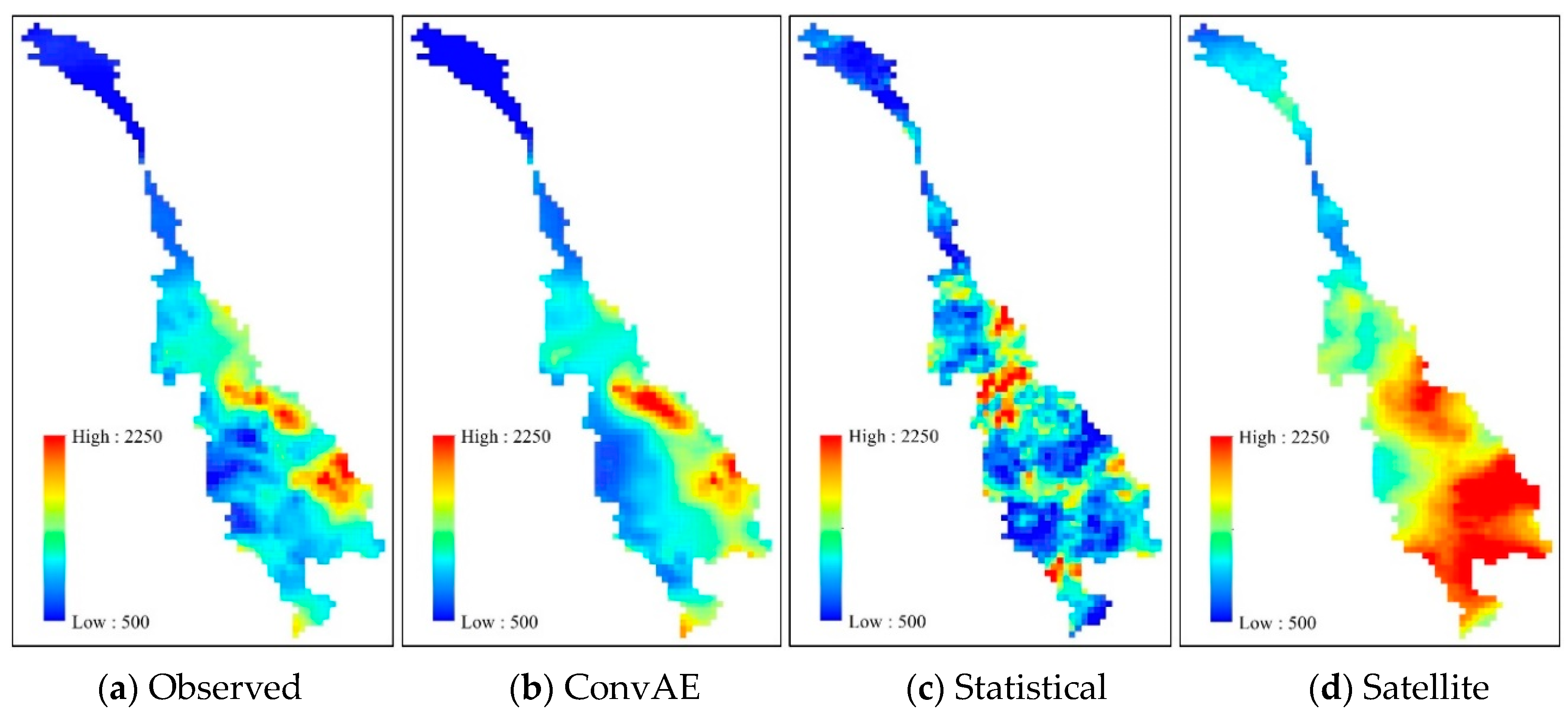
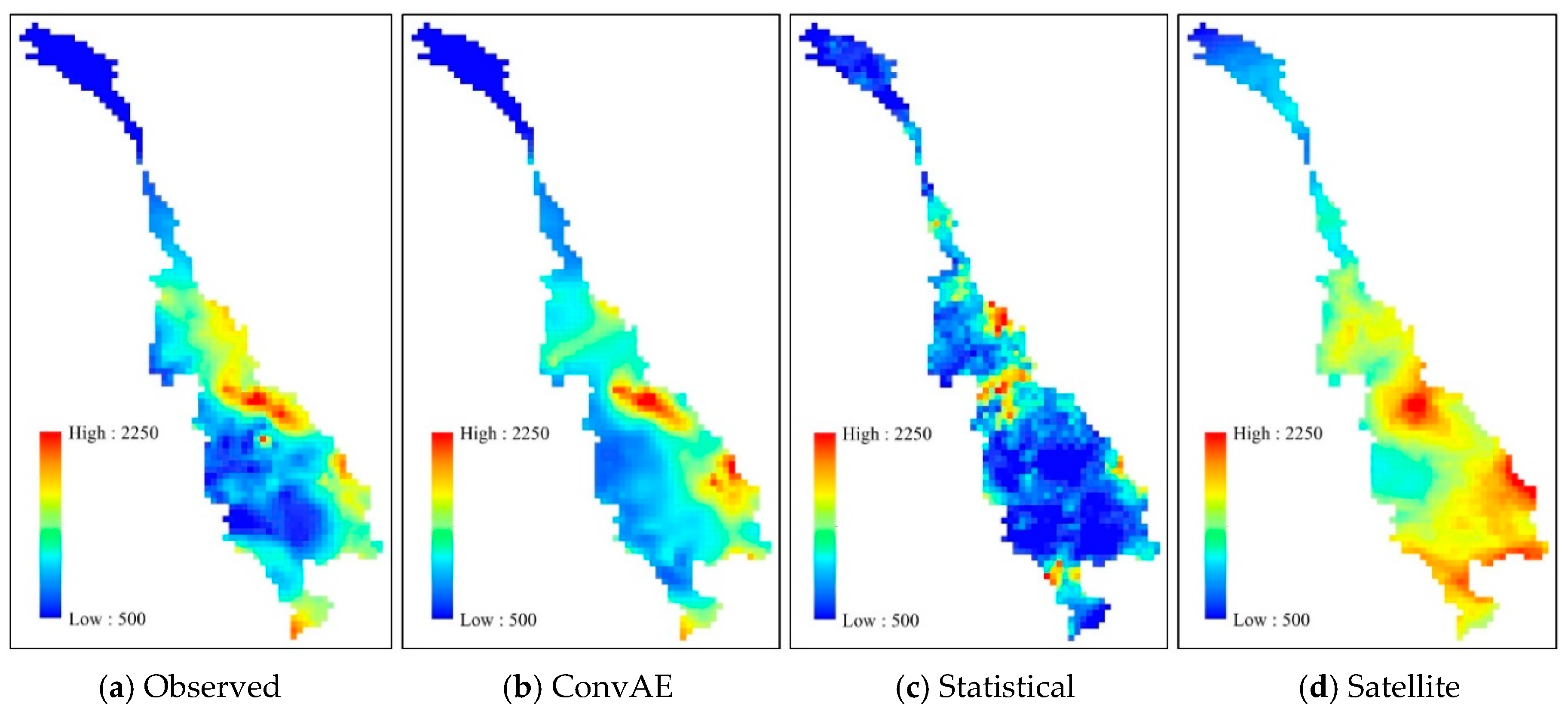
With the visualization of the gridded products, the spatial distribution of the annual precipitation could be clearly identified in Figure 12 and Figure 13. In general, there were significant differences between the precipitation products and the uneven annual rainfall distribution over the Mekong River basin, ranging from roughly 250 mm to well above 2250 mm. Moreover, the LMB received much higher average annual precipitation than the UMB. The recorded information from the observed data revealed that the North-Central of Lao PDR and the eastern mountainous areas bordering Vietnam are the places receiving the largest rainfall of the year (more than 2000 mm).

A similar pattern of rainfall distribution was also noted in the case of the monthly precipitation. Figure 14 illustrates the spatial distribution of the precipitation in August 2014, which is one of the months experiencing the largest precipitation of the year in the Mekong basin. The visualized images again obviously illustrate that satellite-based precipitation products are overestimated in terms of the annual precipitation and monthly precipitation, especially in the LMB. With respect to the two corrected rainfall products, the spatial distribution patterns point out two opposite trends. While the ConvAE model proved a close relationship with the observed rainfall data, the adjusted precipitation from the statistical method demonstrated the opposite trend. Table 4 provides quantitative information on the differences between the precipitation products.

As can be seen in Table 4, the figures again indicate the effectiveness of the ConvAE model in both verification years. The correlation coefficient (Corr) value of the ConvAE model that measures the agreement with observed data in the spatial distribution by pixel-by-pixel was 0.91 and 0.84 for 2014 and 2015, respectively. In addition, other indicators of the ConvAE model—For example, the RMSE of 174 mm, MAD of 134 mm, and bias of 39 mm in 2014—Also demonstrated the smallest pixel-by-pixel difference. For satellite-based precipitation, the overestimation was clearly evident from the MAD and bias indicators (where bias was a positive value). Moreover, the average of the annual rainfall difference with the observed data over the Mekong River basin had a large gap, an amount of 574 mm for 2014 and 448 mm for 2015. However, the satellite-based precipitation products achieved remarkable spatial correlation. The correlation values in the two years of the testing period were 0.61 and 0.63, respectively, which were higher than those given by the statistical methods and smaller than the ConvAE model.

Another important fact was also identified in the case of corrected data from the statistical method. In spite of indicating an impressive temporal correlation compared to the observed data with an NSE value of 0.83 (see Table 3), Table 4 reveals the uncertainty of the statistical method in the spatial distribution, as well as spatial correlation. The correlation values for this method were only 0.32 for 2014 and 0.46 for 2015, which were the lowest values out of the three products mentioned in Table 4. Besides, the bias value is a negative number, which means that the average of the annual precipitation by grid cell of the statistical method is smaller than the observed data, an amount corresponding to −61 mm in 2014 and −226 mm in 2015.

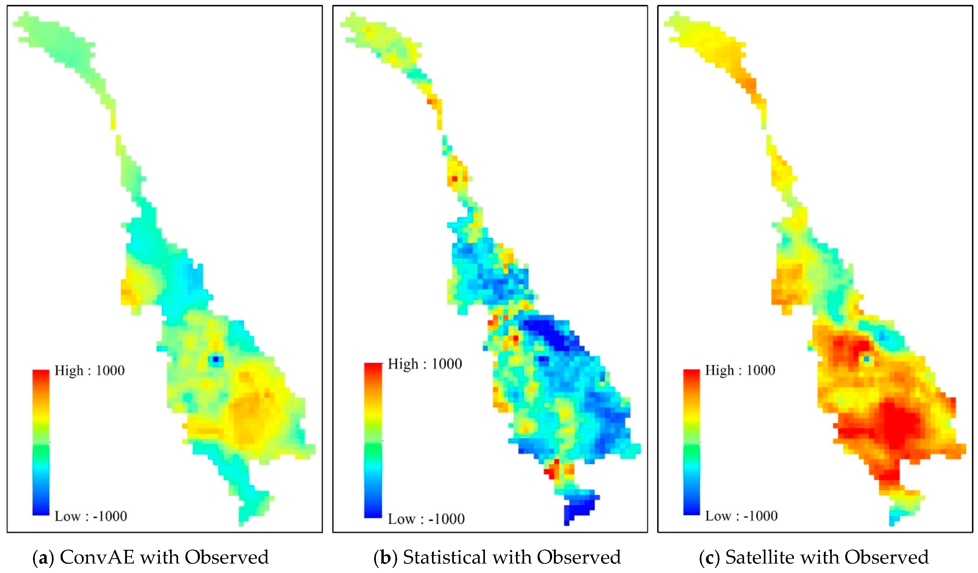
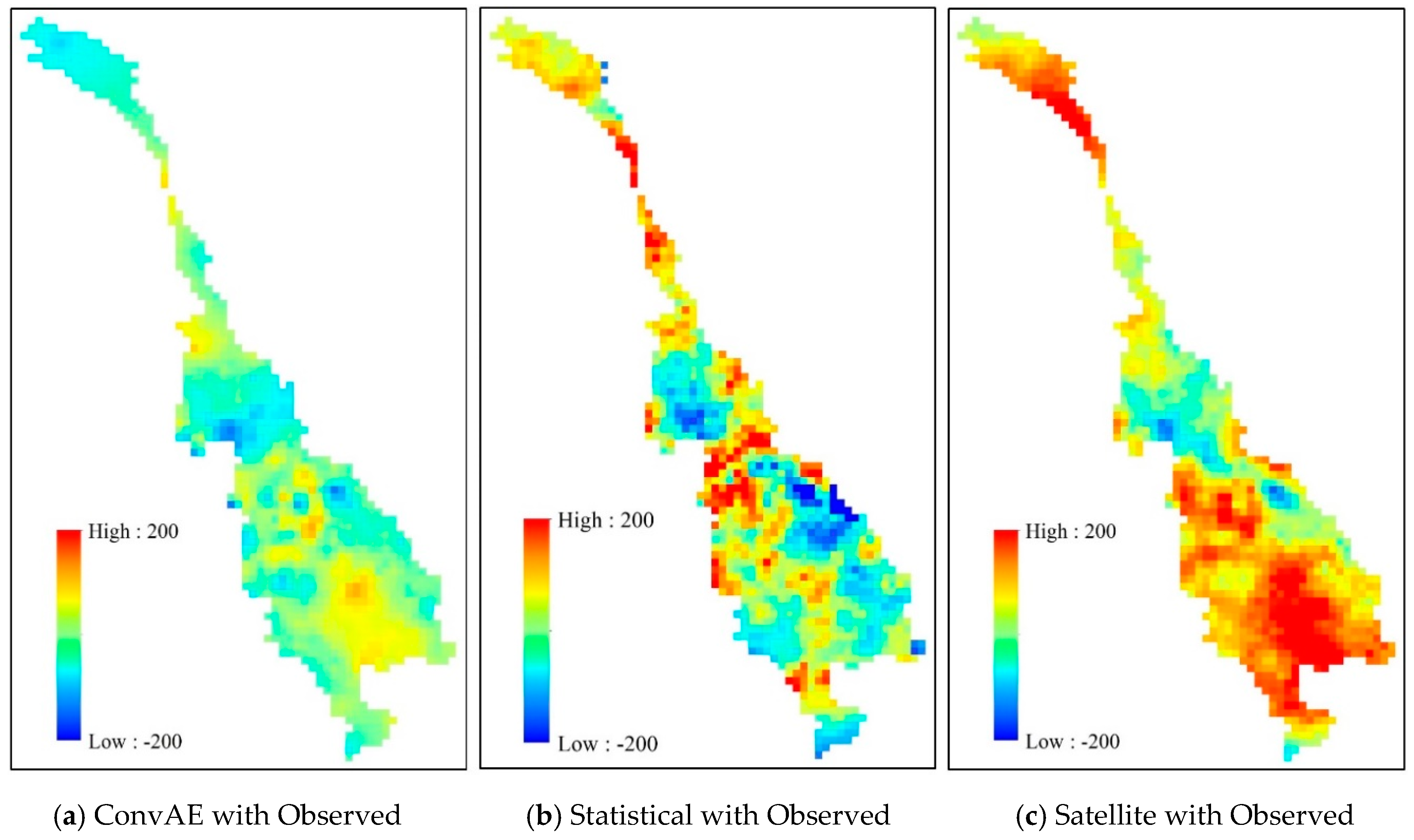
4.4. Spatial Bias Correlation

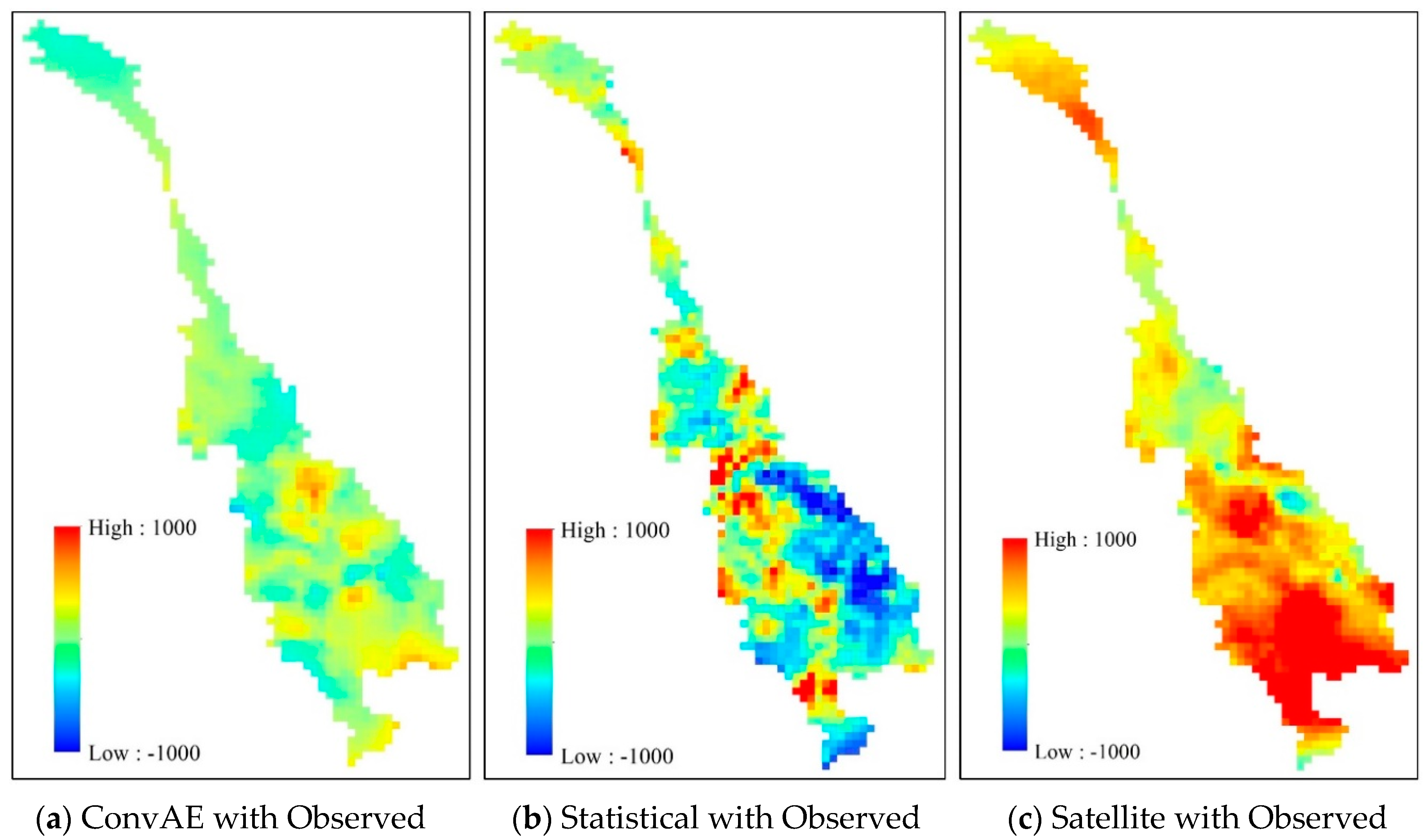
Finally, pixel-by-pixel precipitation differences between the corrected products and observed data are also of interest and have been visualized in Figure 15, Figure 16 and Figure 17.

The spatial bias distribution of the precipitation products is obtained by comparing pixel-by-pixel between the precipitation products and observation data and then calculating the difference of each pair of these pixels. Positive values of the pixels simply implied that the compared precipitation was higher than the observed precipitation, and so on. In order to clearly illustrate the pixel-by-pixel differences between the compared precipitation products and observed data, a fixed scale was applied to visualize the results. This scale ranged from −1000 mm to 1000 mm for the annual rainfall bias (Figure 15 and Figure 16) and ranged from −200 mm to 200 mm for the monthly rainfall bias (Figure 17).

Overall, the ConvAE model demonstrated the lowest bias distribution among the three products described. The satellite-based precipitation again evidently expressed overestimation, especially in the LMB, where the pixel-by-pixel bias of this product was mostly positive, with a difference of more than 1000 mm noted for the annual rainfall. Meanwhile, the instability and uncertainty were recorded in the case of the statistical methods in terms of both the annual rainfall and monthly rainfall. The precipitation spatial bias pattern of this method depicted the considerable differences between the pixels over the Mekong River basin. It can be seen that, despite the facts of the bias value, the average of the pixel-by-pixel difference was not high (see Table 4), with an amount of 37 mm for 2014 and −61 mm for 2015; the spatial bias of the precipitation fluctuated sharply.

In the case of the ConvAE model, there was a satisfactory agreement between the adjusted precipitation and the observed data in the testing phase of the two years. Furthermore, the spatial distribution pattern of the precipitation bias gave information on the pixel-by-pixel difference of the ConvAE model as being negligible compared to the statistical method or satellite-based product. However, the precipitation data of 2015 showed an anomaly of a grid cell, where the adjusted data was much smaller than the observed data (see Figure 16a). This was also the location that recorded unusually heavy rainfall in 2015 (more than 2250 mm) compared to the other precipitation products (see Figure 13). The cause of this anomaly may be the observed data.

5. Conclusions

This paper proposes an effective approach based on the CNN model, called the ConvAE model, to address the problem of daily gridded precipitation bias correction from satellite-derived precipitation data. In addition to the ConvAE model, another bias correction method based on the statistical method, called the standard deviation method, was also introduced in this study. The performance of the bias correction methods was carefully evaluated by comparing the corrected data with observed data in terms of both the temporal correlation and spatial correlation. The Mekong River basin was selected as the case study area, because it is one of the largest river basins in the world, covering six countries (most of which are developing countries). Therefore, reliable information on the precipitation over the Mekong River basin is valuable in forecasting extreme events such as floods or droughts.

With respect to the standard deviation method, the adjusted precipitation indicated a noticeable result in the temporal correlation. However, this model has revealed instability and uncertainty in terms of the probability distribution, spatial correlation, and spatial bias distribution of precipitation. In contrast to the standard deviation method, the ConvAE model demonstrated superior and more stable performances in most comparisons conducted in this study. Moreover, the precipitation spatial distribution patterns illustrated the outstanding performance of the ConvAE model compared to the standard deviation method in describing the spatial relationships between adjacent grid cells. This could be explained by the ConvAE model constructed on the idea of the CNN model, which has proved very effective in the field of computer vision. Meanwhile, the standard deviation method considers pixels as independent values and does not take into account the spatial relationship of precipitation. Another advantage of the ConvAE model is the ability to capture extreme rainfall events and rainfall distribution trends due to the design of architectural layers inside the ConvAE model, i.e., the convolutional and pooling layers.

Despite the fact that the precipitation bias correction problem was effectively solved by the ConvAE model, some limitations need to be considered. The results of this study depend closely on the gridded precipitation data sources. In particular, PERSIANN-CDR is exploited as a satellite-derived precipitation dataset, and APHRODITE is considered as an observed precipitation dataset. Both of these gridded daily precipitation products have the same spatial resolution of 0.25°. APHRODITE is the gridded precipitation product of the international cooperation program; therefore, they are closely related to the data sources provided by the countries in the region of interest. Moreover, precipitation data are usually used in conjunction with hydrological models to simulate rainfall–runoff processes for a specific basin. This is a limitation of this study as a result of the rainfall-runoff process, which has not been illustrated.

For hydrological studies in large areas, such as the Mekong basin, which spans many countries, updating the rainfall data continuously is an important requirement to ensure an accurate rainfall-runoff process simulation. However, it is difficult to construct updated rainfall datasets at the same time because of the close reliance on data collection and the distribution methods of the countries involved. On the other hand, satellite-based precipitation data with various products, availability, and coverage of a large area may be a good suggestion for large study basins, if these data are well-calibrated both spatially and temporally by the proposed technique.

This study is the first step towards enhancing our understanding of the application of deep-learning neural network models to hydrological-related problems. The findings of this study highlighted the potential of the ConvAE model in the daily precipitation bias correction problem. In the context of the APHRODITE project being paused (from 2015), the corrected data source from the ConvAE model promises to be a reliable alternative data source. Furthermore, the ConvAE model could be applied to other satellite-based precipitation products, higher-resolution precipitation data (for example, the spatial resolution of 0.05° and radar data), or other problems related to gridded data.

References

1. Schuurmans, J.M.; Bierkens, M.F.P. Effect of spatial distribution of daily rainfall on interior catchment response of a distributed hydrological model. Hydrol. Earth Syst. Sci. 2007, 11, 677–693. [Google Scholar] [CrossRef] [Green Version]
2. Liu, X.; Yang, T.; Hsu, K.; Liu, C.; Sorooshian, S. Evaluating the streamflow simulation capability of PERSIANN-CDR daily rainfall products in two river basins on the Tibetan Plateau. Hydrol. Earth Syst. Sci. 2017, 21, 169–181. [Google Scholar] [CrossRef] [Green Version]
3. Sun, Q.; Miao, C.; Duan, Q.; Ashouri, H.; Sorooshian, S.; Hsu, K.-L. A review of global precipitation data sets: Data sources, estimation, and intercomparisons. Rev. Geophys. 2018, 56, 79–107. [Google Scholar] [CrossRef] [Green Version]
4. Collischonn, B.; Collischonn, W.; Tucci, C.E.M. Daily hydrological modeling in the Amazon basin using TRMM rainfall estimates. J. Hydrol. 2008, 360, 207–216. [Google Scholar] [CrossRef]
5. López López, P.; Immerzeel, W.W.; Rodríguez Sandoval, E.A.; Sterk, G.; Schellekens, J. Spatial downscaling of satellite-based precipitation and its impact on discharge simulations in the Magdalena river basin in Colombia. Front. Earth Sci. 2018, 6, 68. [Google Scholar] [CrossRef] [Green Version]
6. Huffman, G.J.; Bolvin, D.T.; Nelkin, E.J.; Wolff, D.B.; Adler, R.F.; Gu, G.; Hong, Y.; Bowman, K.P.; Stocker, E.F. The TRMM multisatellite precipitation analysis (TMPA): Quasi-global, multiyear, combined-sensor precipitation estimates at fine scales. J. Hydrometeorol. 2007, 8, 38–55. [Google Scholar] [CrossRef]
7. Hsu, K.-l.; Gao, X.; Sorooshian, S.; Gupta, H.V. Precipitation estimation from remotely sensed information using artificial neural networks. J. Appl. Meteorol. 1997, 36, 1176–1190. [Google Scholar] [CrossRef]
8. Nguyen, P.; Shearer, E.J.; Tran, H.; Ombadi, M.; Hayatbini, N.; Palacios, T.; Huynh, P.; Braithwaite, D.; Updegraff, G.; Hsu, K.; et al. The CHRS data portal, an easily accessible public repository for PERSIANN global satellite precipitation data. Sci. Data 2019, 6, 180296. [Google Scholar] [CrossRef] [Green Version]
9. Funk, C.; Peterson, P.; Landsfeld, M.; Pedreros, D.; Verdin, J.; Shukla, S.; Husak, G.; Rowland, J.; Harrison, L.; Hoell, A.; et al. The climate hazards infrared precipitation with stations—A new environmental record for monitoring extremes. Sci. Data 2015, 2, 150066. [Google Scholar] [CrossRef] [Green Version]
10. Joyce, R.J.; Janowiak, J.E.; Arkin, P.A.; Xie, P. CMORPH: A method that produces global precipitation estimates from passive microwave and infrared data at high spatial and temporal resolution. J. Hydrometeorol. 2004, 5, 487–503. [Google Scholar] [CrossRef]
11. Ashouri, H.; Nguyen, P.; Thorstensen, A.; Hsu, K.-l.; Sorooshian, S.; Braithwaite, D. Assessing the efficacy of high-resolution satellite-based PERSIANN-CDR precipitation product in simulating streamflow. J. Hydrometeorol. 2016, 17, 2061–2076. [Google Scholar] [CrossRef]
12. Miao, C.; Ashouri, H.; Hsu, K.-L.; Sorooshian, S.; Duan, Q. Evaluation of the PERSIANN-CDR daily rainfall estimates in capturing the behavior of extreme precipitation events over China. J. Hydrometeorol. 2015, 16, 1387–1396. [Google Scholar] [CrossRef] [Green Version]
13. Sorooshian, S.; Hsu, K.-L.; Gao, X.; Gupta, H.V.; Imam, B.; Braithwaite, D. Evaluation of PERSIANN system satellite-based estimates of tropical rainfall. Bull. Am. Meteorol. Soc. 2000, 81, 2035–2046. [Google Scholar] [CrossRef] [Green Version]
14. Vu, T.T.; Li, L.; Jun, K.S. Evaluation of multi-satellite precipitation products for streamflow simulations: A case study for the Han River basin in the Korean Peninsula, East Asia. Water 2018, 10, 642. [Google Scholar] [CrossRef] [Green Version]
15. Javanmard, S.; Yatagai, A.; Nodzu, M.I.; BodaghJamali, J.; Kawamoto, H. Comparing high-resolution gridded precipitation data with satellite rainfall estimates of TRMM_3B42 over Iran. Adv. Geosci. 2010, 25, 119–125. [Google Scholar] [CrossRef] [Green Version]
16. Meng, J.; Li, L.; Hao, Z.; Wang, J.; Shao, Q. Suitability of TRMM satellite rainfall in driving a distributed hydrological model in the source region of Yellow River. J. Hydrol. 2014, 509, 320–332. [Google Scholar] [CrossRef]
17. Derin, Y.; Yilmaz, K.K. Evaluation of multiple satellite-based precipitation products over complex topography. J. Hydrometeorol. 2014, 15, 1498–1516. [Google Scholar] [CrossRef] [Green Version]
18. Kim, J.P.; Jung, I.W.; Park, K.W.; Yoon, S.K.; Lee, D. Hydrological utility and uncertainty of multi-satellite precipitation products in the mountainous region of South Korea. Remote Sens. 2016, 8, 608. [Google Scholar] [CrossRef] [Green Version]
19. Chaudhary, S.; Dhanya, C.T. Investigating the Performance of Bias Correction Algorithms on Satellite-Based Precipitation Estimates; SPIE: Bellingham, WA, USA, 2019; Volume 11149. [Google Scholar]
20. Saber, M.; Yilmaz, K.K. Evaluation and bias correction of satellite-based rainfall estimates for modelling flash floods over the mediterranean region: Application to Karpuz River Basin, Turkey. Water 2018, 10, 657. [Google Scholar] [CrossRef] [Green Version]
21. Piani, C.; Haerter, J.O.; Coppola, E. Statistical bias correction for daily precipitation in regional climate models over Europe. Theor. Appl. Climatol. 2010, 99, 187–192. [Google Scholar] [CrossRef] [Green Version]
22. Valdés-Pineda, R.; Demaría, E.M.C.; Valdés, J.B.; Wi, S.; Serrat-Capdevilla, A. Bias correction of daily satellite-based rainfall estimates for hydrologic forecasting in the Upper Zambezi, Africa. Hydrol. Earth Syst. Sci. Discuss. 2016, 2016, 1–28. [Google Scholar] [CrossRef] [Green Version]
23. Pratama, A.W.; Buono, A.; Hidayat, R.; Harsa, H. Bias Correction of Daily Satellite Precipitation Data Using Genetic Algorithm. In Proceedings of the 4th International Symposium on LAPAN-IPB Satellite for Food Security and Environmental Monitoring, Bogor, Indonesia, 9–11 October 2017. IOP Conf. Series Earth Environ. Sci. 2018, 149, 012071. [Google Scholar] [CrossRef]
24. MRC. State of the Basin Report 2018; Mekong River Commission: Vientiane, Laos, 2019. [Google Scholar]
25. Ashouri, H.; Hsu, K.-L.; Sorooshian, S.; Braithwaite, D.K.; Knapp, K.R.; Cecil, L.D.; Nelson, B.R.; Prat, O.P. PERSIANN-CDR: Daily precipitation climate data record from multisatellite observations for hydrological and climate studies. Bull. Am. Meteorol. Soc. 2015, 96, 69–83. [Google Scholar] [CrossRef] [Green Version]
26. Yatagai, A.; Kamiguchi, K.; Arakawa, O.; Hamada, A.; Yasutomi, N.; Kitoh, A. APHRODITE: Constructing a long-term daily gridded precipitation dataset for asia based on a dense network of rain gauges. Bull. Am. Meteorol. Soc. 2012, 93, 1401–1415. [Google Scholar] [CrossRef]
27. Dandridge, C.; Lakshmi, V.; Bolten, J.; Srinivasan, R. Evaluation of satellite-based rainfall estimates in the lower Mekong River basin (Southeast Asia). Remote Sens. 2019, 11, 2709. [Google Scholar] [CrossRef] [Green Version]
28. Try, S.; Lee, G.; Yu, W.; Oeurng, C.; Jang, C. Large-scale flood-inundation modeling in the Mekong River basin. J. Hydrol. Eng. 2018, 23, 05018011. [Google Scholar] [CrossRef]
29. Try, S.; Tanaka, S.; Tanaka, K.; Sayama, T.; Oeurng, C.; Uk, S.; Takara, K.; Hu, M.; Han, D. Comparison of gridded precipitation datasets for rainfall-runoff and inundation modeling in the Mekong River basin. PLoS ONE 2020, 15, e0226814. [Google Scholar] [CrossRef] [Green Version]
30. Yatagai, A.; Arakawa, O.; Kamiguchi, K.; Kawamoto, H.; Nodzu, M.I.; Hamada, A. A 44-year daily gridded precipitation dataset for asia based on a dense network of rain gauges. SOLA 2009, 5, 137–140. [Google Scholar] [CrossRef] [Green Version]
31. Chen, C.-J.; Senarath, S.U.S.; Dima-West, I.M.; Marcella, M.P. Evaluation and restructuring of gridded precipitation data over the greater Mekong subregion. Int. J. Climatol. 2017, 37, 180–196. [Google Scholar] [CrossRef]
32. Hamada, A.; Arakawa, O.; Yatagai, A. An automated quality control method for daily rain-gauge data. Glob. Environ. Res. 2011, 15, 165–172. [Google Scholar]
33. Willmott, C.J.; Rowe, C.M.; Philpot, W.D. Small-Scale Climate Maps: A sensitivity analysis of some common assumptions associated with grid-point interpolation and contouring. Am. Cartogr. 1985, 12, 5–16. [Google Scholar] [CrossRef]
34. MRC. Overview of the Hydrology of the Mekong Basin; Mekong River Commission: Vientiane, Laos, 2005; p. 73. [Google Scholar]
35. MRC. Annual Mekong Flood Report 2010; Mekong River Commission: Vientiane, Laos, 2011; p. 76. [Google Scholar]
36. MRC. Planning Atlas of the Lower Mekong River Basin; Mekong River Commission: Vientiane, Laos, 2011. [Google Scholar]
37. Karpathy, A. CS231n: Convolutional Neural Networks for Visual Recognition. Available online: http://cs231n.github.io/convolutional-networks/ (accessed on 10 September 2019).
38. Hubens, N. Deep Inside: Autoencoders. Available online: https://towardsdatascience.com/deep-inside-autoencoders-7e41f319999f (accessed on 10 January 2020).
39. Chollet, F. Building Autoencoders in Keras. Available online: https://blog.keras.io/building-autoencoders-in-keras.html (accessed on 6 June 2019).
40. Immerzeel, W.W. Bias Correction for Satellite Precipitation Estimation Used by the MRC Mekong Flood Forecasting System; FutureWater Report 94; FutureWater: Wageningen, The Netherlands, 2010. [Google Scholar]
41. Bouwer, L.M.; Aerts, J.C.J.H.; van de Coterlet, G.M.; van de Giesen, N.; Gieske, A.S.M.; Mannaerts, C.M. Evaluating Downscaling Methods for Preparing Global Circulation Model GCM Data for Hydrological Impact Modelling. In Climate Change in Contrasting River Basins: Adaptation Strategies for Water, Food and Environment; Aerts, J.C.J.H., Droogers, P., Eds.; CABI: Wallingford, UK, 2004; pp. 25–47. [Google Scholar]
42. Rossum, G. Python Tutorial; CWI (Centre for Mathematics and Computer Science): Amsterdam, The Netherlands, 1995. [Google Scholar]
43. Van Der Walt, S.; Colbert, S.C.; Varoquaux, G. The NumPy array: A structure for efficient numerical computation. Comput. Sci. Eng. 2011, 13, 22–30. [Google Scholar] [CrossRef] [Green Version]
44. McKinney, W. Data Structures for Statistical Computing in Python. In Proceedings of the 9th Python in Science Conference, Austin, TX, USA, 28 June–3 July 2020; pp. 51–56. [Google Scholar]
45. Hunter, J.D. Matplotlib: A 2D graphics environment. Comput. Sci. Eng. 2007, 9, 90–95. [Google Scholar] [CrossRef]
46. Chollet, F. Keras. Available online: https://github.com/fchollet/keras (accessed on 6 June 2019).
47. Abadi, M.; Agarwal, A.; Barham, P.; Brevdo, E.; Chen, Z.; Citro, C.; Corrado, G.S.; Davis, A.; Dean, J.; Devin, M.; et al. TensorFlow: Large-scale machine learning on heterogeneous distributed systems. arXiv 2016, arXiv:1603.04467. [Google Scholar]
48. Google. Colaboratory: Frequently Asked Questions. Available online: https://research.google.com/colaboratory/faq.html (accessed on 6 June 2019).
49. Simonyan, K.; Zisserman, A. Very deep convolutional networks for large-scale image recognition. arXiv 2014, arXiv:1409.1556. [Google Scholar]
50. Ronneberger, O.; Fischer, P.; Brox, T. U-Net: Convolutional networks for biomedical image segmentation. arXiv 2015, arXiv:1505.04597. [Google Scholar]
51. Rosebrock, A. Keras Conv2D and Convolutional Layers. Available online: https://www.pyimagesearch.com/2018/12/31/keras-conv2d-and-convolutional-layers/ (accessed on 10 January 2020).
52. Brownlee, J. A Gentle Introduction to Pooling Layers for Convolutional Neural Networks. Available online: https://machinelearningmastery.com/pooling-layers-for-convolutional-neural-networks/ (accessed on 15 January 2020).
53. Kingma, D.P.; Ba, J. Adam: A method for stochastic optimization. arXiv 2014, arXiv:1412.6980. [Google Scholar]
54. Srivastava, N.; Hinton, G.; Krizhevsky, A.; Sutskever, I.; Salakhutdinov, R. Dropout: A simple way to prevent neural networks from overfitting. J. Mach. Learn. Res. 2014, 15, 1929–1958. [Google Scholar] [CrossRef]
55. Taylor, K.E. Summarizing multiple aspects of model performance in a single diagram. J. Geophys. Res. Atmos. 2001, 106, 7183–7192. [Google Scholar] [CrossRef]
56. Rochford, P. SkillMetrics. Available online: https://github.com/PeterRochford/SkillMetrics (accessed on 20 January 2020).
Figure 1. Mekong River basin [24].
Remotesensing 12 02731 g001
Figure 2. Spatial distribution of the precipitation of two gridded products in the Mekong basin in 2000. APHRODITE: Asian Precipitation-Highly Resolved Observational Data Integration towards Evaluation and PERSIANN-CDR: Precipitation Estimation from Remotely Sensed Information using Artificial Neural Networks-Climate Data Record.
Remotesensing 12 02731 g002
Figure 3. Mean annual rainfall of the Mekong River basin from 1998 to 2015.
Remotesensing 12 02731 g003
Figure 4. Box plot of the mean annual rainfall over the Mekong River basin from 1998 to 2015.
Remotesensing 12 02731 g004
Figure 5. Illustration for an autoencoder architecture [39].
Remotesensing 12 02731 g005
Figure 6. Convolutional autoencoder (ConvAE) model the structure for the precipitation bias correction problem. Here, “100 × 60 × 1” refers to “height × width × depth”. With the 2D data, the default value of depth is 1.
Remotesensing 12 02731 g006
Figure 7. Statistical properties of a grid cell in the Mekong basin.
Remotesensing 12 02731 g007
Figure 8. Comparing the correlation of the monthly total precipitation of the data sources over the Mekong basin during the testing period.
Remotesensing 12 02731 g008
Figure 9. Probability distribution of the total precipitation by grid cells in 2014.
Remotesensing 12 02731 g009
Figure 10. Probability distribution of the total precipitation by grid cells in 2015.
Remotesensing 12 02731 g010
Figure 11. Taylor diagram showing the correlation coefficient, standard deviation, and root mean square deviation (RMSD) from the precipitation products based on the observed, ConvAE, statistic, and satellite, respectively.
Remotesensing 12 02731 g011
Figure 12. Spatial distribution pattern of the precipitation products in 2014.
Remotesensing 12 02731 g012
Figure 13. Spatial distribution pattern of the precipitation products in 2015.
Remotesensing 12 02731 g013
Figure 14. Spatial distribution pattern of the precipitation products in August 2014.
Remotesensing 12 02731 g014
Figure 15. Spatial bias distribution pattern of the precipitation products compared to the observed data in 2014.
Remotesensing 12 02731 g015
Figure 16. Spatial bias distribution pattern of the precipitation products compared to the observed data in 2015.
Remotesensing 12 02731 g016
Figure 17. Spatial bias distribution pattern of the precipitation products compared to the observed data in August 2014.
Remotesensing 12 02731 g017