Identifying Soil Erosion Processes in Alpine Grasslands on Aerial Imagery with a U-Net Convolutional Neural Network


Abstract
:
1. Introduction
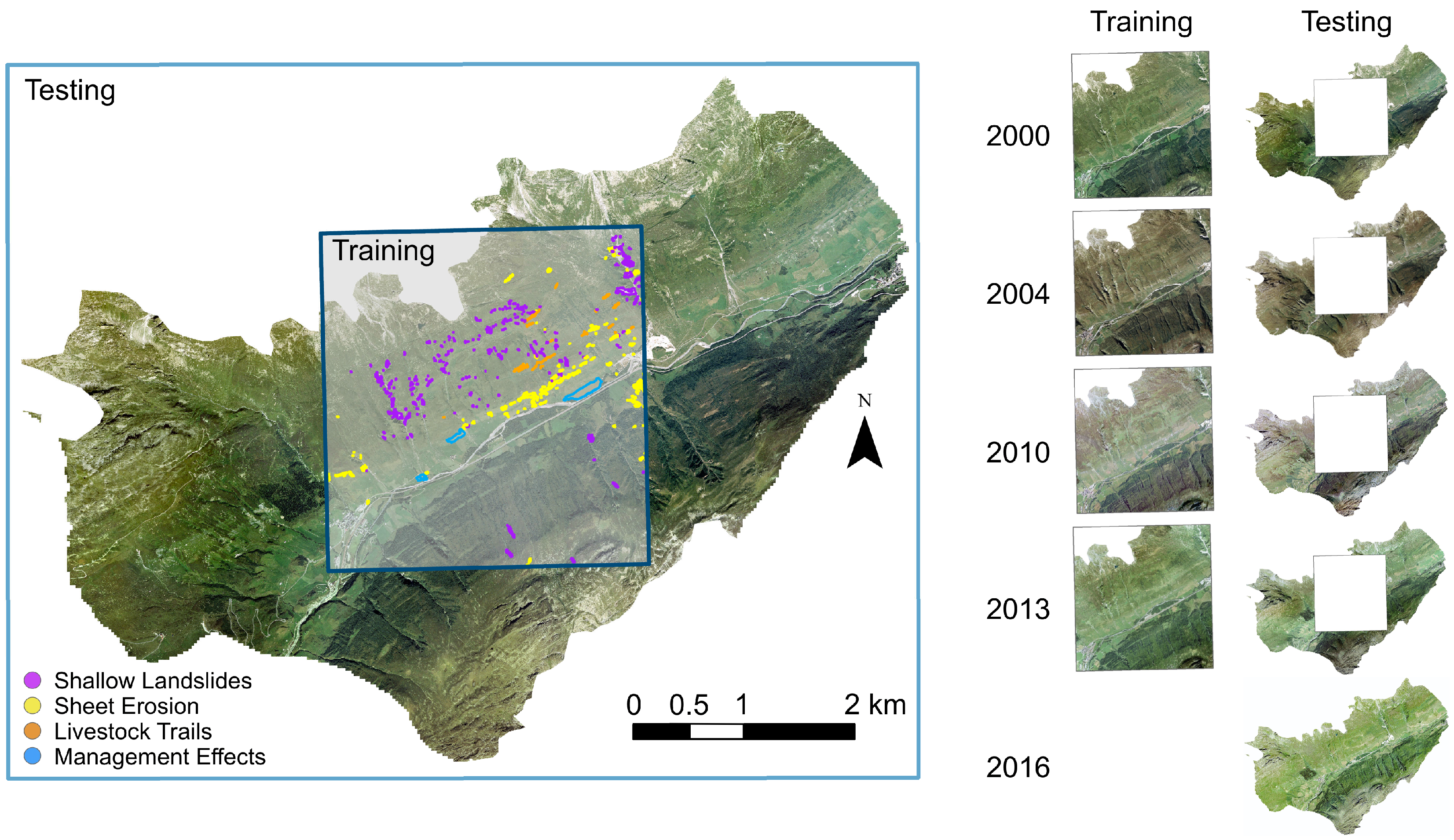
2. Study Area
3. Data Sets
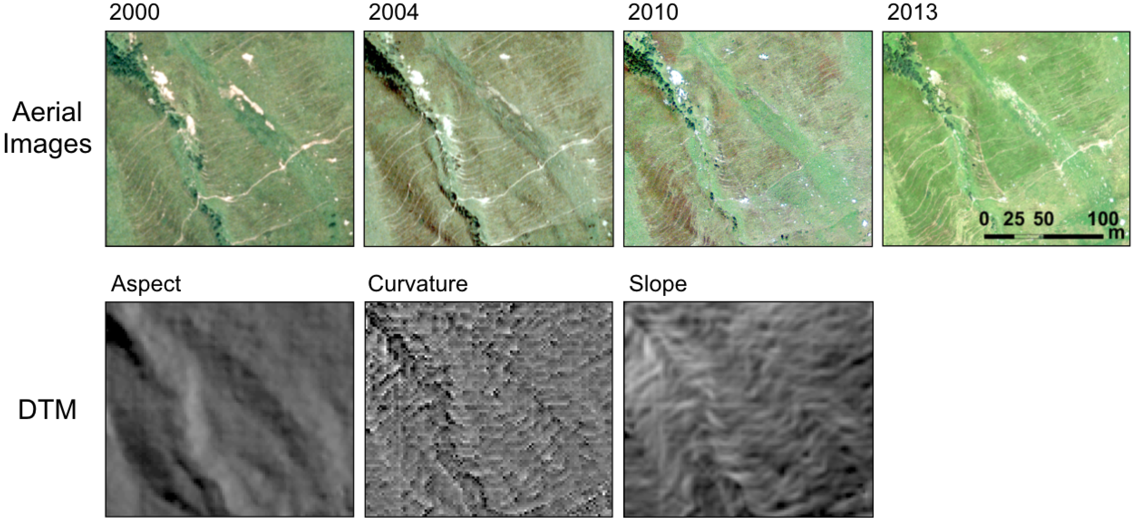
3.1. Aerial Imagery
3.2. Digital Terrain Model
3.3. Training Data
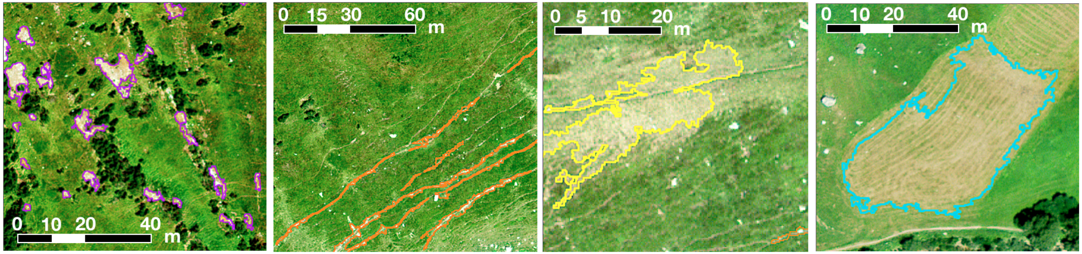
3.3.1. Training Labels
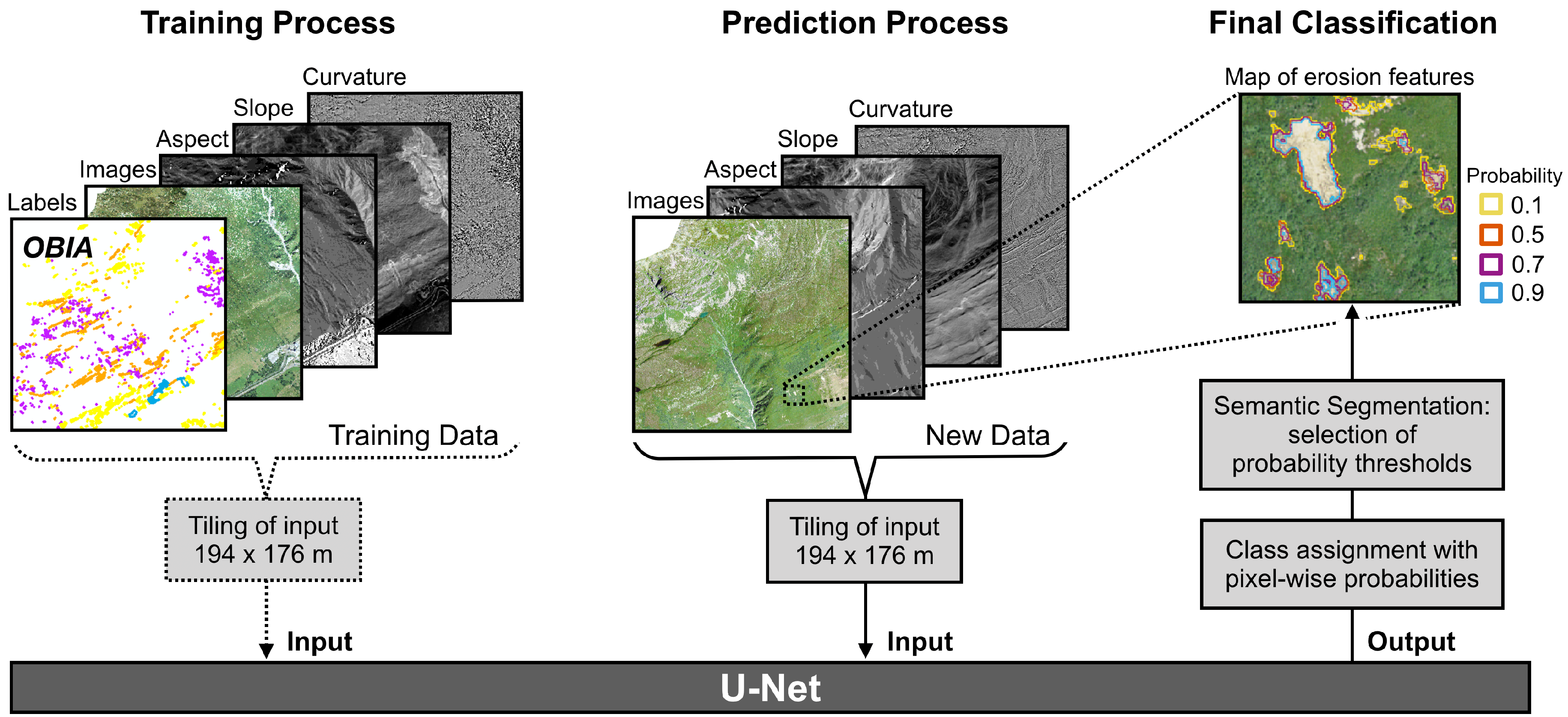
4. Methodology
4.1. Object-Based Image Analysis
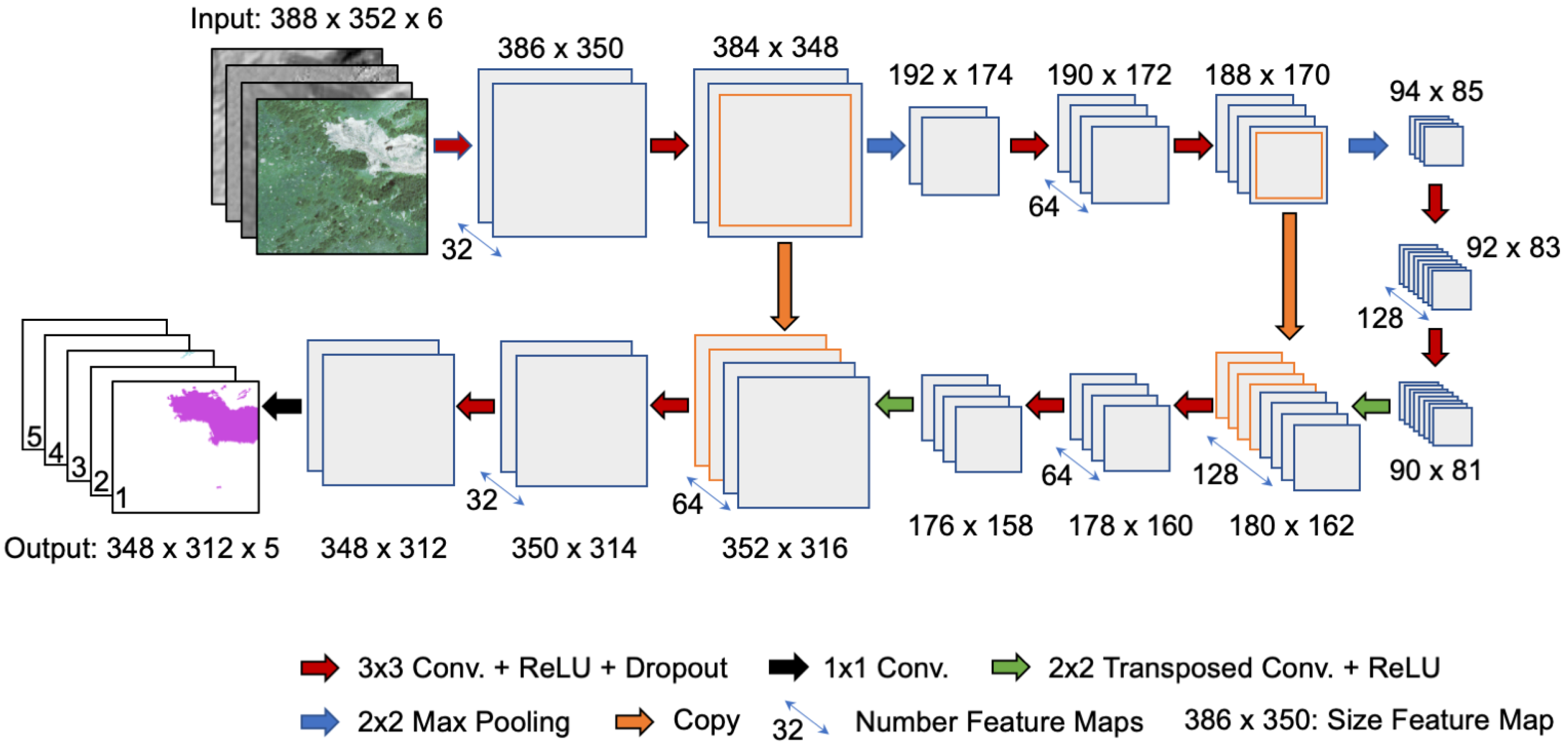
4.2. Neural Network Architecture
4.3. Training Process
4.4. Details on the Evaluation
5. Results and Discussion
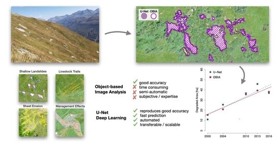
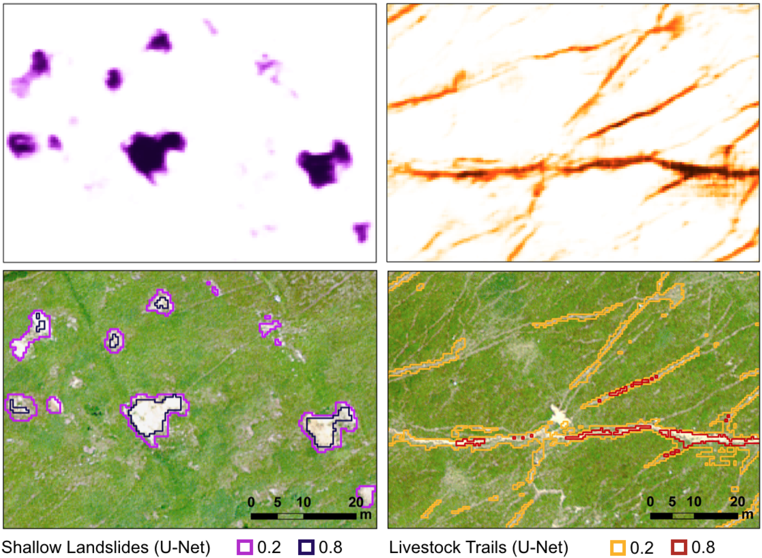
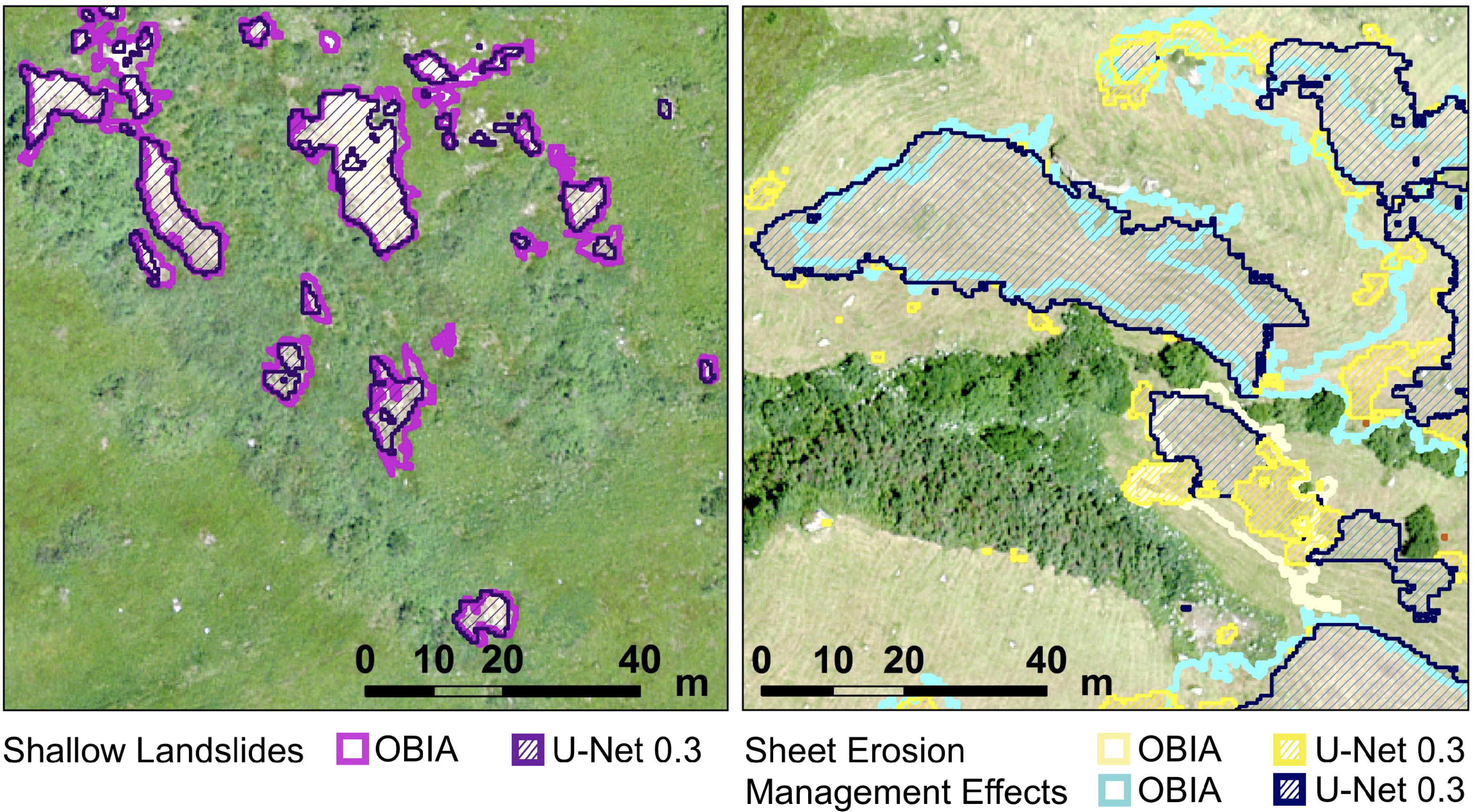
5.1. Segmentation of Soil Erosion Sites
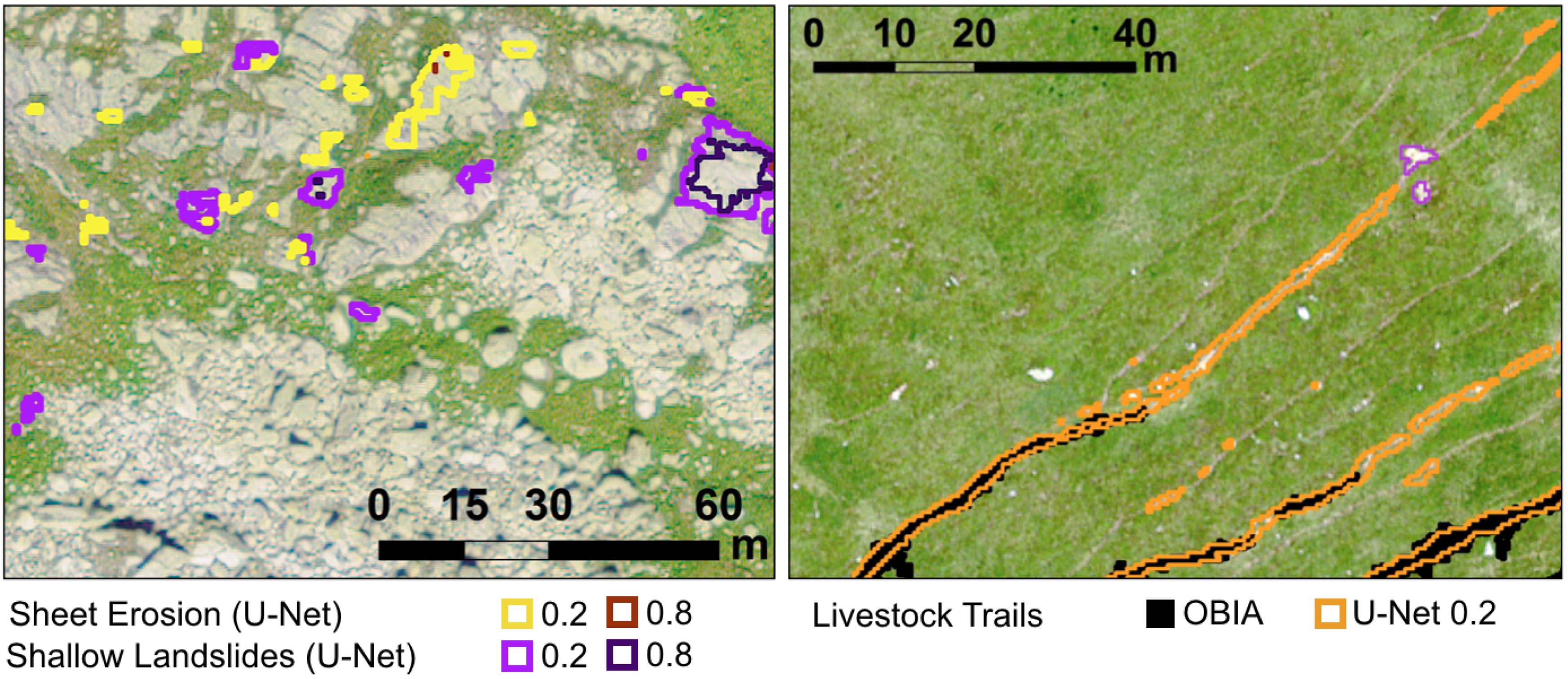
5.2. Threshold Selection
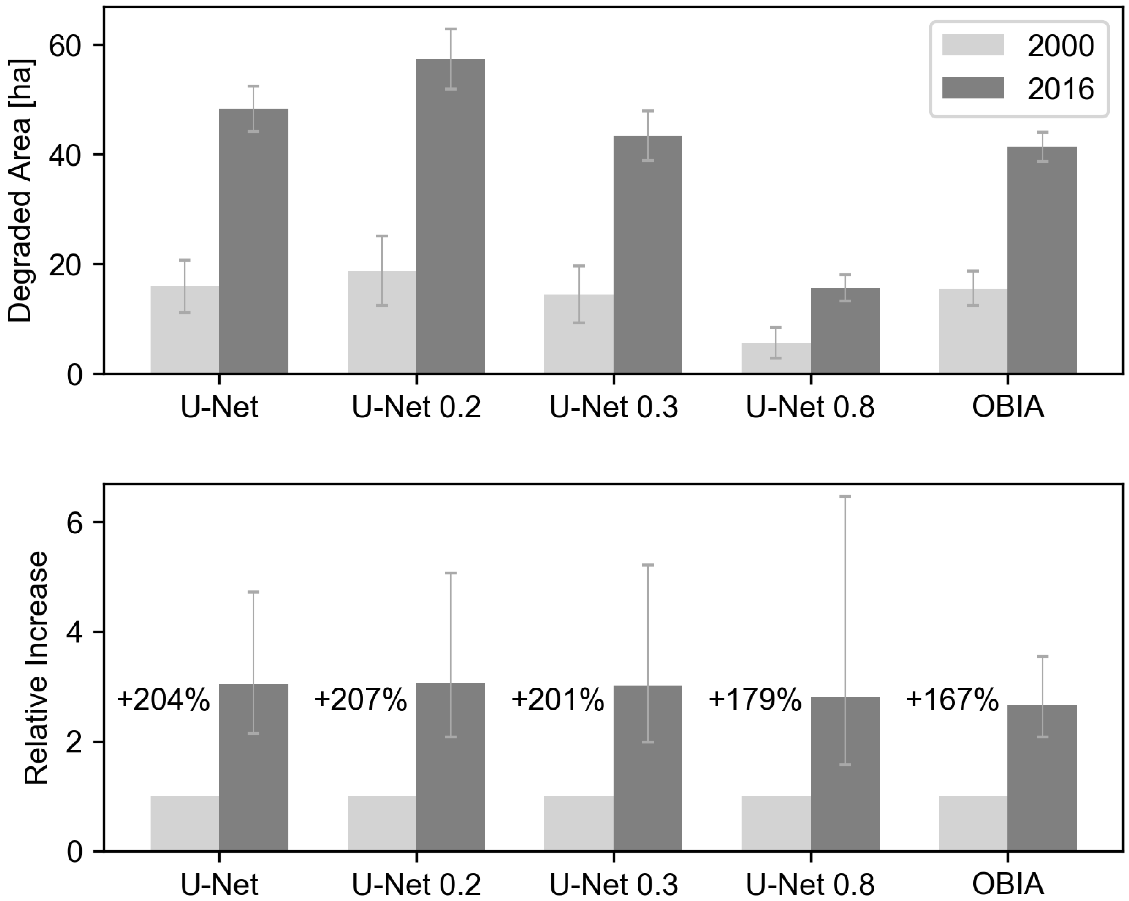
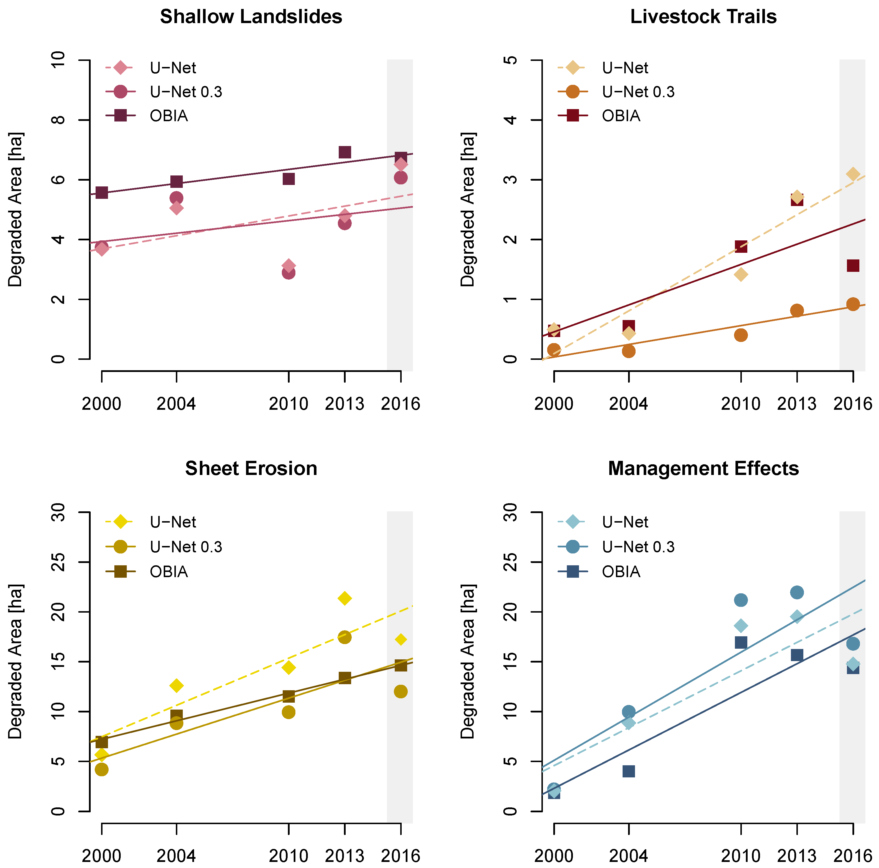
5.3. Trend Analysis of Soil Erosion Sites
5.4. Deep Learning and OBIA
6. Conclusions
Supplementary Materials
Author Contributions
Funding
Acknowledgments
Conflicts of Interest
Abbreviations
| OBIA | Object-based image analysis |
| DTM | Digital terrain model |
| RGB | Red, Green and Blue spectral bands |
| CNN | Convolutional Neural Networks |
| U-Net | Name of Convolutional Neural Network architecture |
| GPU | Graphics Processing Unit |
| UAV | Unmanned Aerial Vehicle |
References
- EEA. Regional Climate Change and Adaptation—The Alps Facing The Challenge of Changing Water Resources; Technical Report 8; European Environmental Agency: Copenhagen, Denmark, 2009. [Google Scholar]
- Fuhrer, J.; Beniston, M.; Fischlin, A.; Frei, C.; Goyette, S.; Jasper, K.; Pfister, C. Climate risks and their impact on agriculture and forests in Switzerland. Clim. Chang. 2006, 79, 79–102. [Google Scholar] [CrossRef] [Green Version]
- Meusburger, K.; Alewell, C. Impacts of anthropogenic and environmental factors on the occurrence of shallow landslides in an alpine catchment (Urseren Valley, Switzerland). Nat. Hazards Earth Syst. Sci. 2008, 8, 509–520. [Google Scholar] [CrossRef] [Green Version]
- Nearing, M.; Pruski, F.; O’Neal, M. Expected climate change impacts on soil erosion rates: A review. J. Soil Water Conserv. 2004, 59, 43–50. [Google Scholar]
- Scheurer, K.; Alewell, C.; Bänninger, D.; Burkhardt-holm, P. Climate and land-use changes affecting river sediment and brown trout in alpine countries—A review. Environ. Sci. Pollut. Res. 2009, 16, 232–242. [Google Scholar] [CrossRef] [Green Version]
- Tasser, E.; Mader, M.; Tappeiner, U. Effects of land use in alpine grasslands on the probability of landslides. Basic Appl. Ecol. 2003, 4, 271–280. [Google Scholar] [CrossRef]
- Zweifel, L.; Meusburger, K.; Alewell, C. Spatio-temporal pattern of soil degradation in a Swiss Alpine grassland catchment. Remote Sens. Environ. 2019, 235, 111441. [Google Scholar] [CrossRef]
- Apollo, M.; Andreychouk, V.; Bhattarai, S.S. Short-term impacts of livestock grazing on vegetation and track formation in a high mountain environment: A case study from the Himalayan Miyar Valley (India). Sustainability 2018, 10, 951. [Google Scholar] [CrossRef] [Green Version]
- Torresani, L.; Wu, J.; Masin, R.; Penasa, M.; Tarolli, P. Estimating soil degradation in montane grasslands of North-eastern Italian Alps (Italy). Heliyon 2019, 5, e01825. [Google Scholar] [CrossRef] [Green Version]
- Wiegand, C.; Geitner, C. Shallow erosion in grassland areas in the Alps. What we know and what we need to investigate further. In Challenges for Mountain Regions: Tackling Complexity; Boehlau Verlag: Wien, Austria, 2010; pp. 76–83. [Google Scholar]
- Alder, S.; Prasuhn, V.; Liniger, H.; Herweg, K.; Hurni, H.; Candinas, A.; Gujer, H.U. A high-resolution map of direct and indirect connectivity of erosion risk areas to surface waters in Switzerland-A risk assessment tool for planning and policy-making. Land Use Policy 2015, 48, 236–249. [Google Scholar] [CrossRef]
- Bircher, P.; Liniger, H.P.; Prasuhn, V. Comparing different multiple flow algorithms to calculate RUSLE factors of slope length (L) and slope steepness (S) in Switzerland. Geomorphology 2019, 346, 106850. [Google Scholar] [CrossRef]
- Meusburger, K.; Bänninger, D.; Alewell, C. Estimating vegetation parameter for soil erosion assessment in an alpine catchment by means of QuickBird imagery. Int. J. Appl. Earth Obs. Geoinf. 2010, 12, 201–207. [Google Scholar] [CrossRef]
- Meusburger, K.; Steel, A.; Panagos, P.; Montanarella, L.; Alewell, C. Spatial and temporal variability of rainfall erosivity factor for Switzerland. Hydrol. Earth Syst. Sci. 2012, 16, 167–177. [Google Scholar] [CrossRef] [Green Version]
- Prasuhn, V.; Liniger, H.; Gisler, S.; Herweg, K.; Candinas, A.; Clément, J.P. A high-resolution soil erosion risk map of Switzerland as strategic policy support system. Land Use Policy 2013, 32, 281–291. [Google Scholar] [CrossRef]
- Schmidt, S.; Alewell, C.; Meusburger, K. Mapping spatio-temporal dynamics of the cover and management factor (C-factor) for grasslands in Switzerland. Remote Sens. Environ. 2018, 211, 89–104. [Google Scholar] [CrossRef]
- Schmidt, S.; Alewell, C.; Meusburger, K. Monthly RUSLE soil erosion risk of Swiss grasslands. J. Maps 2019, 15, 247–256. [Google Scholar] [CrossRef] [Green Version]
- Schmidt, S.; Tresch, S.; Meusburger, K. Modification of the RUSLE slope length and steepness factor (LS-factor) based on rainfall experiments at steep alpine grasslands. MethodsX 2019, 6, 219–229. [Google Scholar] [CrossRef]
- Fischer, F.K.; Kistler, M.; Brandhuber, R.; Maier, H.; Treisch, M.; Auerswald, K. Validation of official erosion modelling based on high-resolution radar rain data by aerial photo erosion classification. Earth Surf. Proc. Land 2018, 43, 187–194. [Google Scholar] [CrossRef]
- Alewell, C.; Borrelli, P.; Meusburger, K.; Panagos, P. Using the USLE: Chances, challenges and limitations of soil erosion modelling. Int. Soil Water Conserv. Res. 2019, 7, 203–225. [Google Scholar] [CrossRef]
- D’Oleire-Oltmanns, S.; Marzolff, I.; Peter, K.D.; Ries, J.B. Unmanned aerial vehicle (UAV) for monitoring soil erosion in Morocco. Remote Sens. 2012, 4, 3390–3416. [Google Scholar] [CrossRef] [Green Version]
- Eisank, C.; Hölbling, D.; Friedl, B.; Chin, Y. Expert knowledge for object-based landslide mapping in Taiwan. South-Eastern Eur. J. Earth Observ. 2014, 3, 347–350. [Google Scholar]
- Guzzetti, F.; Mondini, A.C.; Cardinali, M.; Fiorucci, F.; Santangelo, M.; Chang, K.T. Landslide inventory maps: New tools for an old problem. Earth-Sci. Rev. 2012, 112, 42–66. [Google Scholar] [CrossRef] [Green Version]
- Hölbling, D.; Friedl, B.; Eisank, C. An object-based approach for semi-automated landslide change detection and attribution of changes to landslide classes in northern Taiwan. Earth Sci. Inform. 2015, 8, 327–335. [Google Scholar] [CrossRef] [Green Version]
- Hölbling, D.; Betts, H.; Spiekermann, R.; Phillips, C. Identifying spatio-temporal landslide hotspots on North Island, New Zealand, by analyzing historical and recent aerial photography. Geosciences 2016, 6, 48. [Google Scholar] [CrossRef] [Green Version]
- Hölbling, D.; Abad, L.; Dabiri, Z.; Prasicek, G.; Tsai, T.t.; Argentin, A.l. Mapping and analyzing the evolution of the Butangbunasi landslide using Landsat time series with respect to heavy rainfall events during Typhoons. Appl. Sci. 2020, 10, 630. [Google Scholar] [CrossRef] [Green Version]
- Martha, T.R.; Kerle, N.; van Westen, C.J.; Jetten, V.; Vinod Kumar, K. Object-oriented analysis of multi-temporal panchromatic images for creation of historical landslide inventories. ISPRS J. Photogramm. Remote Sens. 2012, 67, 105–119. [Google Scholar] [CrossRef]
- Shruthi, R.B.V.; Kerle, N.; Jetten, V. Object-based gully feature extraction using high spatial resolution imagery. Geomorphology 2011, 134, 260–268. [Google Scholar] [CrossRef]
- Wang, B.; Zhang, Z.; Wang, X.; Zhao, X.; Yi, L.; Hu, S. Object-based mapping of gullies using optical images: A case study in the black soil region, Northeast of China. Remote Sens. 2020, 12, 487. [Google Scholar] [CrossRef] [Green Version]
- Wiegand, C.; Rutzinger, M.; Heinrich, K.; Geitner, C. Automated extraction of shallow erosion areas based on multi-temporal ortho-imagery. Remote Sens. 2013, 5, 2292–2307. [Google Scholar] [CrossRef] [Green Version]
- Ma, L.; Liu, Y.; Zhang, X.; Ye, Y.; Yin, G.; Johnson, B.A. Deep learning in remote sensing applications: A meta-analysis and review. ISPRS J. Photogramm. Remote Sens. 2019, 152, 166–177. [Google Scholar] [CrossRef]
- Heydari, S.S.; Mountrakis, G. Meta-analysis of deep neural networks in remote sensing: A comparative study of mono-temporal classification to support vector machines. ISPRS J. Photogramm. Remote Sens. 2019, 152, 192–210. [Google Scholar] [CrossRef]
- Huang, B.; Zhao, B.; Song, Y. Urban land-use mapping using a deep convolutional neural network with high spatial resolution multispectral remote sensing imagery. Remote Sens. Environ. 2018, 214, 73–86. [Google Scholar] [CrossRef]
- Yuan, Q.; Shen, H.; Li, T.; Li, Z.; Li, S.; Jiang, Y.; Xu, H.; Tan, W.; Yang, Q.; Wang, J.; et al. Deep learning in environmental remote sensing: Achievements and challenges. Remote Sens. Environ. 2020, 241, 111716. [Google Scholar] [CrossRef]
- Ronneberger, O.; Fischer, P.; Brox, T. U-net: Convolutional networks for biomedical image segmentation. In Proceedings of the Medical Image Computing and Computer-assisted intervention—MICCAI 2015, Munich, Germany, 5–9 October 2015; Volume 9351, pp. 234–241. [Google Scholar]
- Yuan, M.; Liu, Z.; Wang, F. Using the wide-range attention u-net for road segmentation. Remote Sens. Lett. 2019, 10, 506–515. [Google Scholar] [CrossRef]
- Zhang, Z.; Liu, Q.; Wang, Y. Road Extraction by Deep Residual U-Net. IEEE Geosci. Remote Sens. Lett. 2018, 15, 749–753. [Google Scholar] [CrossRef] [Green Version]
- Alshaikhli, T.; Liu, W.; Maruyama, Y. Automated method of road extraction from aerial images using a deep convolutional neural network. Appl. Sci. 2019, 9, 4825. [Google Scholar] [CrossRef] [Green Version]
- Wulamu, A.; Shi, Z.; Zhang, D.; He, Z. Multiscale Road Extraction in Remote Sensing Images. Comput. Intel. Neurosci. 2019, 2019, 1–9. [Google Scholar] [CrossRef] [Green Version]
- Xu, Y.; Wu, L.; Xie, Z.; Chen, Z. Building extraction in very high resolution remote sensing imagery using deep learning and guided filters. Remote Sens. 2018, 10, 144. [Google Scholar] [CrossRef] [Green Version]
- Yi, Y.; Zhang, Z.; Zhang, W.; Zhang, C.; Li, W.; Zhao, T. Semantic segmentation of urban buildings from VHR remote sensing imagery using a deep convolutional neural network. Remote Sens. 2019, 11, 1774. [Google Scholar] [CrossRef] [Green Version]
- Ivanovsky, L.; Khryashchev, V.; Pavlov, V.; Ostrovskaya, A. Building detection on aerial images using U-NET neural networks. In Proceedings of the Conference of Open Innovation Association, FRUCT, Moscow, Russia, 8–12 April 2019; pp. 116–122. [Google Scholar]
- Mboga, N.; Georganos, S.; Grippa, T.; Lennert, M.; Vanhuysse, S.; Wolff, E. Fully convolutional networks and geographic object-based image analysis for the classification of VHR imagery. Remote Sens. 2019, 11, 597. [Google Scholar] [CrossRef] [Green Version]
- Yang, J.; Guo, J.; Yue, H.; Liu, Z.; Hu, H.; Li, K. CDnet: CNN-based cloud detection for remote sensing imagery. IEEE Trans. Geosci. Remote Sens. 2019, 57, 6195–6211. [Google Scholar] [CrossRef]
- Flood, N.; Watson, F.; Collett, L. Using a U-net convolutional neural network to map woody vegetation extent from high resolution satellite imagery across Queensland, Australia. Int. J. Appl. Earth Obs. 2019, 82, 101897. [Google Scholar] [CrossRef]
- Kattenborn, T.; Eichel, J.; Fassnacht, F.E. Convolutional Neural Networks enable efficient, accurate and fine-grained segmentation of plant species and communities from high-resolution UAV imagery. Sci. Rep. 2019, 9, 17656. [Google Scholar] [CrossRef] [PubMed]
- Hamdi, Z.M.; Brandmeier, M.; Straub, C. Forest damage assessment using deep learning on high resolution remote sensing data. Remote Sens. 2019, 11, 1976. [Google Scholar] [CrossRef] [Green Version]
- Baumhoer, C.A.; Dietz, A.J.; Kneisel, C.; Kuenzer, C. Automated extraction of antarctic glacier and ice shelf fronts from Sentinel-1 imagery using deep learning. Remote Sens. 2019, 11, 2529. [Google Scholar] [CrossRef] [Green Version]
- Bundzel, M.; Jaščur, M.; Kováč, M.; Lieskovský, T.; Sinčák, P.; Tkáčik, T. Semantic segmentation of airborne lidar data in maya archaeology. Remote Sens. 2020, 12, 1–22. [Google Scholar] [CrossRef]
- Wyss, R. Die Urseren-Zone—Lithostratigraphie und Tektonik. Eclogae Geol. Hel. 1986, 79, 731–767. [Google Scholar]
- IUSS Working Group WRB. World Reference Base for Soil Resources; IUSS Working Group WRB: Wageningen, The Netherlands, 2006; pp. 1–128. [Google Scholar]
- Alewell, C.; Egli, M.; Meusburger, K. An attempt to estimate tolerable soil erosion rates by matching soil formation with denudation in Alpine grasslands. J. Soils Sediments 2015, 15, 1383–1399. [Google Scholar] [CrossRef] [Green Version]
- Swisstopo. Swissimage. Das Digitale Farborthophotomosaik der Schweiz; Swisstopo: Wabern, Switzerland, 2010.
- Swisstopo. SwissALTI3D. Das hoch aufgelöste Terrainmodell der Schweiz; Swisstopo: Wabern, Switzerland, 2014.
- Kingma, D.P.; Ba, J.L. Adam: A method for stochastic optimization. In Proceedings of the 3rd International Conference on Learning Representations, ICLR 2015, San Diego, CA, USA, 7–9 May 2015; pp. 1–15. [Google Scholar]
- Abadi, M.; Barham, P.; Chen, J.; Chen, Z.; Davis, A.; Dean, J.; Devin, M.; Ghemawat, S.; Irving, G.; Isard, M.; et al. TensorFlow: A System for Large-Scale Machine Learning. In Proceedings of the 12th USENIX Symposium on Operating Systems Design and Implementation (OSDI ’16), Savannah, GA, USA, 1 November 2016; pp. 265–283. [Google Scholar]
- Akeret, J.; Chang, C.; Lucchi, A.; Refregier, A. Radio frequency interference mitigation using deep convolutional neural networks. Astron. Comput. 2017, 18, 35–39. [Google Scholar] [CrossRef] [Green Version]
- Alewell, C.; Meusburger, K.; Brodbeck, M.; Bänninger, D. Methods to describe and predict soil erosion in mountain regions. Landsc. Urban Plan. 2008, 88, 46–53. [Google Scholar] [CrossRef]
- Meusburger, K.; Alewell, C. Soil Erosion in the Alps; Federal Office for the Environment FOEN: Bern, Switzerland, 2014; p. 118. [Google Scholar]
- Konz, N.; Baenninger, D.; Konz, M.; Nearing, M.; Alewell, C. Process identification of soil erosion in steep mountain regions. Hydrol. Earth Syst. Sci. 2010, 14, 675–686. [Google Scholar] [CrossRef] [Green Version]
- Konz, N.; Prasuhn, V.; Alewell, C. On the measurement of alpine soil erosion. Catena 2012, 91, 63–71. [Google Scholar] [CrossRef]
- Guirado, E.; Tabik, S.; Alcaraz-Segura, D.; Cabello, J.; Herrera, F. Deep-learning Versus OBIA for scattered shrub detection with Google Earth Imagery: Ziziphus lotus as case study. Remote Sens. 2017, 9, 1220. [Google Scholar] [CrossRef] [Green Version]
- Fu, Y.; Liu, K.; Shen, Z.; Deng, J.; Gan, M.; Liu, X.; Lu, D.; Wang, K. Mapping impervious surfaces in town-rural transition belts using China’s GF-2 imagery and object-based deep CNNs. Remote Sens. 2019, 11, 280. [Google Scholar] [CrossRef] [Green Version]
- Zhang, C.; Sargent, I.; Pan, X.; Li, H.; Gardiner, A.; Hare, J.; Atkinson, P.M. An object-based convolutional neural network (OCNN) for urban land use classification. Remote Sens. Environ. 2018, 216, 57–70. [Google Scholar] [CrossRef] [Green Version]
- Lu, H.; Ma, L.; Fu, X.; Liu, C.; Wang, Z.; Tang, M.; Li, N. Landslides information extraction using Object-Oriented Image Analysis paradigm based on Deep Learning and Transfer Learning. Remote Sens. 2020, 12, 752. [Google Scholar] [CrossRef] [Green Version]
- Prakash, N.; Manconi, A.; Loew, S. Mapping landslides on EO data: Performance of deep learning models vs. Traditional machine learning models. Remote Sens. 2020, 12, 346. [Google Scholar] [CrossRef] [Green Version]
- Ghorbanzadeh, O.; Blaschke, T.; Gholamnia, K.; Meena, S.R.; Tiede, D.; Aryal, J. Evaluation of different machine learning methods and deep-learning convolutional neural networks for landslide detection. Remote Sens. 2019, 11, 196. [Google Scholar] [CrossRef] [Green Version]
- Pan, X.; Zhao, J.; Xu, J. An object-based and heterogeneous segment filter convolutional neural network for high-resolution remote sensing image classification. Int. J. Remote Sens. 2019, 40, 5892–5916. [Google Scholar] [CrossRef]


| Data Set | Derivative | Spectral Bands | Spatial Res. | Recording Date | |
|---|---|---|---|---|---|
| Aerial Image | Red, Green, Blue | 0.5 m | 24 August | 2000 | |
| Red, Green, Blue | 0.5 m | 9 September | 2004 | ||
| Red, Green, Blue | 0.25 m | 20 July | 2010 | ||
| Red, Green, Blue | 0.25 m | 1 August | 2013 | ||
| Red, Green, Blue | 0.25 m | 20 July | 2016 | ||
| Digital Terrain | Slope | 2 m | |||
| Model (DTM) | Aspect | 2 m | |||
| Curvature | 2 m |
| Scores | U-Net |
|---|---|
| Recall | 84% |
| Precision | 73% |
| F | 78% |
Publisher’s Note: MDPI stays neutral with regard to jurisdictional claims in published maps and institutional affiliations. |
© 2020 by the authors. Licensee MDPI, Basel, Switzerland. This article is an open access article distributed under the terms and conditions of the Creative Commons Attribution (CC BY) license (http://creativecommons.org/licenses/by/4.0/).
Share and Cite
Samarin, M.; Zweifel, L.; Roth, V.; Alewell, C. Identifying Soil Erosion Processes in Alpine Grasslands on Aerial Imagery with a U-Net Convolutional Neural Network. Remote Sens. 2020, 12, 4149. https://0-doi-org.brum.beds.ac.uk/10.3390/rs12244149
Samarin M, Zweifel L, Roth V, Alewell C. Identifying Soil Erosion Processes in Alpine Grasslands on Aerial Imagery with a U-Net Convolutional Neural Network. Remote Sensing. 2020; 12(24):4149. https://0-doi-org.brum.beds.ac.uk/10.3390/rs12244149
Chicago/Turabian StyleSamarin, Maxim, Lauren Zweifel, Volker Roth, and Christine Alewell. 2020. "Identifying Soil Erosion Processes in Alpine Grasslands on Aerial Imagery with a U-Net Convolutional Neural Network" Remote Sensing 12, no. 24: 4149. https://0-doi-org.brum.beds.ac.uk/10.3390/rs12244149