Article

Improved Estimation of Regional Surface Mass Variations from GRACE Intersatellite Geopotential Differences Using a Priori Constraints

1
School of Geodesy and Geomatics, Wuhan University, Wuhan 430079, China
2
MOE Key Laboratory of Fundamental Physical Quantities Measurement, Institute of Geophysics, School of Physics, Huazhong University of Science and Technology, Wuhan 430074, China
3
Center for Space Research, University of Texas at Austin, Austin, TX 78759, USA
*
Author to whom correspondence should be addressed.
Remote Sens. 2020, 12(16), 2553; https://0-doi-org.brum.beds.ac.uk/10.3390/rs12162553
Submission received: 24 June 2020 / Revised: 30 July 2020 / Accepted: 6 August 2020 / Published: 8 August 2020
(This article belongs to the Special Issue Geodesy for Gravity and Height Systems)

Abstract

:
We presented an improved method for estimation of regional surface mass variations from the Gravity Recovery and Climate Experiment (GRACE)-derived precise intersatellite geopotential differences using a priori constraints. An alternative analytic formula was proposed to incorporate the K-band ranging (KBR) range rate into the improved energy balance equation, and precise geopotential differences were estimated from GRACE Level-1B data based on the remove-compute-restore (RCR) technique, which avoids the long-wavelength gravity signals being absorbed by empirical parameters. To reduce the ill condition for inversion of regional mass variations from geopotential differences, a priori information from hydrological models was used to construct the constraint equations, and the optimal regularization parameters were adaptively determined based on iterative least-squares estimation. To assess our improved method, a case study of regional mass variations’ inversion was carried out over South America on 2° × 2° grids at monthly intervals from January 2005 to December 2010. The results show that regional mascon solutions inverted from geopotential differences estimated by the RCR technique using hydrological models as a priori constraints can retain more signal energy and enhance regional mass variation inversion. The spatial distributions and annual amplitudes of geopotential difference-based regional mascon solutions agree well with the official GRACE mascon solutions, although notable differences exist in spatial patterns and trends, especially in small basins. In addition, our improved method can robustly estimate the mascon solutions, which are less affected by the a priori information. The results from the case study have clearly demonstrated the feasibility and effectiveness of the proposed method.

1. Introduction

Over the past 16 plus years, surface mass variations derived from the Gravity Recovery and Climate Experiment (GRACE) satellite gravimetry has significantly improved our ability to study the terrestrial water cycle, ice sheets and mountain glacier mass balance, sea level change, and ocean bottom pressure variations, as well as to understand responses to changes in the global climate system [1,2]. The traditional approach for modeling surface mass variations is based on the time-variable gravity field, which is represented by spherical harmonic (SH) basis functions [3,4], and surface mass variations obtained from GRACE Level-2 monthly SH solutions, e.g., the Center for Space Research (CSR), Geoforschungszentrum (GFZ), and Jet Propulsion Laboratory (JPL) published RL05/06 SH solutions [5,6,7,8,9] can reach a spatial resolution of ~300 km [10,11], or even better than 300 km through enhanced processing techniques [12,13]. However, without using constraints or a priori information, GRACE SH solutions have typically suffered from poor observability of east-west gradients, resulting in the longitudinal stripes that are conventionally removed by spatial filtering [14,15]. Spatial smoothing and filtering have a tendency to attenuate the real geophysical signals, which further degrades the spatial resolution of GRACE-estimated surface mass variations [16,17,18]. Therefore, several dedicated correction methods [17,19,20,21] were developed for improving the effective spatial resolution of GRACE SH solutions, which can help detect surface mass variations at small regional scales [13].
In addition to the traditional SH basis functions approach, an alternative way to estimate surface mass variations from GRACE is to use the mass concentration (mascon) approach. The mascon approach can estimate surface mass variations directly from intersatellite K-band ranging (KBR) measurements (Level-1B data), and the longitudinal stripes are suppressed by applying constraints [11,22,23,24,25,26,27]. Because the mascon parameters are nonlinear functions of the KBR observations, the final mascon solutions are conventionally estimated by the least-squares iterative algorithm, in which the partial derivatives of the KBR observations with respect to mascon parameters are computed by the dynamic method. Theoretically, unconstrained global mascon solutions are equivalent to unconstrained SH solutions, but mascon parameters are particularly easy to use with various types of constraints, which result in less signal loss and spatial leakage [11,22,25]. Several institutes, including JPL, CSR and the Goddard Space Flight Center (GSFC), have generated global GRACE mascon solutions (e.g., JPL and CSR RL05/06 mascon solutions [24,25,26,28], and GSFC mascon solutions [11,29]) based on the dynamic method, which can be directly applied to the analysis of surface mass variations. In addition, several studies fit mascon parameters to SH coefficients from monthly GRACE SH solutions [30,31,32,33], but these are not true mascon solutions in the sense that there are no direct connections between mascon parameters and KBR observations [24,26].
Due to the nonlinear relationship between mascon parameters and KBR observations, as well as the time-consuming calculations of the dynamic method, an alternative estimation of mascon parameters from GRACE intersatellite geopotential differences based on the energy balance approach was widely studied in the past decade [34,35,36,37,38]. The advantages of this method are twofold. First, the mascon parameters are linear functions of the geopotential differences, and can be conveniently estimated in least-squares solutions without any iterative corrections. Second, the GRACE intersatellite geopotential differences are in situ gravimetric observables, as a quantity with explicit geophysical interpretation [34,39], which can directly reflect surface mass variations compared with that of geometric KBR data. In general, there are two steps for inferring these mascon solutions. The first step is to estimate intersatellite geopotential differences from GRACE KBR observations and global positioning system (GPS) orbits, along with non-gravitational accelerations using the energy balance equation. The second step is to convert intersatellite geopotential differences into surface mass variations, which are usually expressed in terms of the equivalent water height (EWH) through a downward continuation process.
Some previous studies have been done on precise estimation of in situ intersatellite geopotential differences from GRACE Level-1B data. Based on numerical approximation of the energy balance equation presented by Jekeli [40], Han et al. [41] attempted to adjust the KBR range-rate, GPS orbit, and accelerometer data simultaneously through a non-linear least-squares estimation with fixed constraints; Tangdamrongsub et al. [38] employed the same strategy to estimate geopotential differences but via stochastic constraints. In order to further improve the accuracy of geopotential differences, Ramillien et al. [36] computed the potential rotation term by considering the static part of the gravitational; Guo et al. [42] presented a more accurate formulation of the potential rotation term, which includes the contributions of time-variable components of the gravitational potential. As the energy integral does not explicitly contain the precise KBR range-rate measurements, Shang et al. [39] introduced an analytic alignment equation to incorporate the residual KBR range-rate into the energy balance equation based on the reconstruction of the related reference orbit, which is more accurate than using the approximate correction terms presented by Jekeli [40]. However, intersatellite geopotential differences estimated from the above procedures may still contain systematic errors from the KBR measurements. The most common method to reduce the systematic errors is to absorb these errors by using empirical parameters (e.g., two cycle-per-revolution (CPR) parameters used in Han et al. [41] and Tangdamrongsub et al. [38], four CPR parameters used in Ramillien et al. [37]), but these empirical parameters would also weaken the temporal gravity signals, especially the long-wavelength components [37,39,43,44]. For example, several studies (e.g., Ramillien et al. [37], Frédéric Frappart et al. [43], and Ramillien et al. [44]) used the low degrees of SH solutions to complement the missing long-wavelength information of surface mass variations. Unlike the previous studies, we will employ the remove-compute-restore (RCR) technique to retain the temporal gravity signals to the full extent, and extract precise intersatellite geopotential differences based on an improved energy balance equation.
In the second step, the intersatellite geopotential differences are expressed as a function of surface mass variations, and are conventionally downward-continued from satellite altitude to the Earth’s surface by Newton’s formula of gravitational potential [34,35,36,37,38]. However, the noises in intersatellite geopotential differences will be amplified, and the estimation of mascon parameters is a well-known ill-posed problem. Therefore, regularization strategies have been employed to find numerically stable mascon solutions from intersatellite geopotential differences, either based on singular value decomposition (SVD) and L-curve analysis [36], or by introducing spatial constraints [37], and these regularization methods were verified from the inversion of surface mass variations over South America at 10- to 30-day intervals using different sizes of blocks. Besides, Han et al. [34] introduced a priori information equation to estimate the mascon parameters by an iterative least-squares estimation. Tangdamrongsub et al. [38] constructed space-domain and space-time covariance functions using a priori hydrological knowledge to obtain stable mascon solutions, in which the optimal regularization parameters were determined based on the L-curve criterion. Because the L-curve criterion is an empirical method to find the optimal regularization parameters, it is often a tedious job to solve for the mascon solutions with certain time intervals from a long period of GRACE data. In order to adaptively determine the optimal regularization parameters according to the data themselves, inspired by the work of Han et al. [34], we will make full use of a priori information to obtain the stable mascon solutions based on the iterative least-squares estimation.
Mascon solutions do not suffer from spectral truncation effects like in GRACE SH solutions, and can offer surface mass variations with higher spatio-temporal resolution at the regional scale [25,34,36,38]. Compared with the inversion of global mascon solutions, estimation of regional surface mass variations in the form of regional mascon solutions are computationally convenient because they can be estimated from a small subset of the global GRACE KBR data. In this study, we focused on the inversion of regional mascon solutions from GRACE intersatellite geopotential differences using a priori constraints. Firstly, we present an alternative analytic formula to incorporate the KBR range-rate into the energy balance equation, and estimate the precise in situ intersatellite geopotential differences from GRACE Level-1B data based on the RCR technique using the energy integral. Secondly, we employ an adaptive algorithm to determine the optimal regularization parameters based on the iterative least-squares method using hydrological model outputs as a priori constraints. Finally, a case study of regional mass variations’ inversion over South America on 2° × 2° geographic grids at monthly intervals from January 2005 to December 2010 is presented, and our solutions are compared to the official GRACE mascon solutions to demonstrate the feasibility of the proposed methods.

2. Methods and Data

2.1. Improved Energy Balance Equation

Due to the approximation of the potential rotation term in the energy integral developed by Jekeli [40], we follow a more accurate formulation of the potential rotation term presented by Guo et al. [42], and an improved energy balance equation can be formulated in the geocentric inertial frame for a single satellite as follows [39]:
V E = 1 2 | r ˙ | 2 w · ( r × r ˙ ) t 0 t a · ( r ˙ w × r ) d t E 0 ,
where V E is the Earth’s gravitational potential; r and r ˙ are the orbit position and velocity in the inertial frame; w is the angular velocity vector of the Earth-fixed frame with respect to the inertial frame; a = V T + f includes the non-conservative force f , as well as the forces derived from high-frequency time-variable gravitational potential V T (due to N-body perturbation, solid Earth tides, ocean tides, pole tides, atmosphere and ocean signals, etc.); the integration in Equation (1) is from the initial time t 0 to t ; and E 0 is a constant of integration.
The in situ intersatellite geopotential difference between GRACE’s two satellites can be derived according to Equation (1) as:
V 12 E = V 2 E V 1 E = 1 2 ( r ˙ 2 + r ˙ 1 ) · r ˙ 12 w · ( r 2 × r ˙ 2 r 1 × r ˙ 1 ) t 0 t ( a 2 · ( r ˙ 2 w × r 2 ) a 1 · ( r ˙ 1 w × r 1 ) ) d t E 12 0 ,
where the subscripts represent two GRACE satellites (‘1’, ‘2’) and their difference (‘12’). Because the energy integral in Equation (2) does not explicitly contain the KBR range-rate measurements, Shang et al. [39] introduced an alignment equation to update the relative velocity vector r ˙ 12 by using the precise range-rate ρ ˙ . Unlike the alignment equation, we simply decompose the relative velocity vector r ˙ 12 into the line-of-sight (LOS) direction and its orthogonal direction, which is in the plane containing the relative position vector r 12 and relative velocity vector r ˙ 12 , and the range-rate ρ ˙ can be incorporated into the first term on the right side of Equation (2) (called kinetic energy term) as follows:
E 12 k = 1 2 ( r ˙ 2 + r ˙ 1 ) · ( ( r ˙ 12 · e 12 ) e 12 + ( r ˙ 12 ( r ˙ 12 · e 12 ) e 12 ) ) = 1 2 ( r ˙ 2 + r ˙ 1 ) · ( ρ ˙ e 12 + ( r ˙ 12 ( r ˙ 12 · e 12 ) e 12 ) ) ,
where E 12 k is the difference of the kinetic energy between the two satellites, the range-rate ρ ˙ = r ˙ 12 · e 12 , and e 12 = r 12 | r 12 | is the LOS unit vector. Our numerical test based on one month of GRACE data showed that the root-mean-square (RMS) difference between Equation (3) and the alignment equation [39] for estimation of E 12 k is less than 5.0 × 10⁻⁷ m2/s2, which is negligible compared with the GRACE measurement accuracy.

2.2. Inversion Method of Regional Surface Mass Variations

The intersatellite geopotential difference V 12 E obtained from Equation (2) mainly includes static gravitational potential due to the solid Earth and time-variable part due to mass redistributions (including continental hydrology, postglacial rebound, earthquake, etc.). Here, we introduce a static reference geopotential U , and intersatellite geopotential difference due to mass changes, which is estimated from T 12 = V 12 E U 12 , and U 12 is the geopotential difference computed by the reference geopotential U . Then, the residual geopotential difference T 12 can be used to invert regional surface mass variations. The study area can be divided into regular geographical grids, and the center of the j th block is located at the colatitudes θ j and the longitude λ j , and its surface area is δ S j = R 2 Δ θ Δ λ sin θ j , in which R is the mean Earth’s radius, and Δ θ and Δ λ are the sampling angle intervals along the latitude and the longitude, respectively. For a given period Δ t = t t 0 , the surface mass change of the j th block δ m j can be expressed as:
δ m j ( θ j , λ j , Δ t ) = ρ w δ S j δ h j ( θ j , λ j , Δ t ) ,
where ρ w is the mean density of water (1000 kg/m3), and δ h j is the unknown EWH at location ( θ j , λ j ) during the period Δ t .
Based on Newton’s law of gravitation, the relationship between surface mass variations and geopotential difference at the satellite’s altitude can be expressed as follows [34,36,38]:
T 12 = G j = 1 M ( 1 l 2 j 1 l 1 j ) δ m j ,
in which G is the Newtonian constant (6.673 × 10⁻¹¹ m3kg−1s−2), M is the total number of blocks in the study area, and l 1 j and l 2 j are distances between each GRACE satellite (‘1’, ‘2’) and the center of the j th block, which can be expressed as [36]:
1 l 1 , 2 j = 1 R n = 0 ( R r 1 , 2 ) n + 1 P n ( cos ψ 1 , 2 j ) ,
where P n is the Legendre polynomial of order n , and c o s ψ 1 , 2 j = c o s θ j c o s θ 1 , 2 + s i n θ j s i n θ 1 , 2 c o s ( λ j λ 1 , 2 ) , ( r 1 , θ 1 , λ 1 ) , and ( r 2 , θ 2 , λ 2 ) are the geocentric radius, geocentric co-latitude, and longitude for each GRACE satellite (‘1’, ‘2’). Substituting Equation (4) and Equation (6) into Equation (5), and considering the load effects caused by the surface mass variations, we can obtain the observation equations to estimate regional mass variations from geopotential difference observables as follows:
T 12 = G ρ w R j = 1 M n = 0 δ S j δ h j ( 1 + k n ) ( ( R r 2 ) n + 1 P n ( c o s ψ 2 j ) ( R r 1 ) n + 1 P n ( c o s ψ 1 j ) ) ,
where k n are the load Love numbers that account for the elastic deformation potential for a viscoelastic Earth, and the values of load Love numbers were adopted from Wahr et al. [3]. It should be pointed out that in order to avoid the influence of edge effects on the regional mascon solutions, the boundary of calculation region should be expanded appropriately.

2.3. Adaptive Estimation Method Using a Priori Constraints

As it is known, recovering surface mass variations from geopotential differences based on Equation (7) is an ill-posed problem, because the noises will be amplified when geopotential difference data are downward continued from the satellite altitude to the Earth’s surface. Several studies employed regularization techniques (e.g., SVD, L-curve) [36], spatial constraints [37] and a priori constraints [38] to reduce the ill condition in the regional mass variation solution from GRACE. However, it is a tedious job to find the optimal regularization parameters for massive GRACE data processing. In this study, we used a priori constraints based on geophysical information (e.g., hydrological models) to stabilize the ill-posed problem, and adaptively determined the optimal regularization parameters from the data themselves based on the iterative least-squares estimation method.
The linear observation equation from Equation (7) for estimating surface mass variations can be expressed as follows:
y = A x + e ,     e ~ ( 0 , σ y 2 I ) ,
where y is the observation vector of residual geopotential differences, A is the design matrix, x is the EWH parameter vector to be estimated, e is the residual vector with zero expectation and identity cofactor matrix, and σ y 2 is the error variance of geopotential differences.
In order to stabilize the solutions, a stochastic model for the unknown parameter vector x is introduced based on the use of a priori information. Here, assuming that we have an a priori expectation x 0 and covariance matrix C x for the parameter vector x , the a priori information equations can be expressed as follows:
x 0 = I x x + e 0 ,     e 0 ( 0 , C x ) ,
where e 0 is the residual vector with zero expectation and covariance matrix C x , I x is the identity matrix associated to the parameter vector x .
The idea of regularization is to find the balance between the minimum norm of the residuals and that of the vector of unknown parameters relative to the a priori values. By minimizing A x y 2 + α x x 0 2 = m i n , the optimal solution can be determined as:
x ^ = ( A T A + α σ y 2 C x 1 ) 1 ( A T y + α σ y 2 C x 1 x 0 ) ,
in which α is a regularization parameter to balance the weights between the observations and the a priori information. Because both the regularization parameter α and error variance σ y 2 are unknown in Equation (10), we can estimate them together through variance component estimation [45] as follows:
α ^ σ ^ y 2 = y T y x ^ T ( 2 A T y ) + x ^ T ( A T A ) x ^ n o b s ( x 0 x ^ ) T C x 1 ( x 0 x ^ ) ,
in which n o b s is the number of observations.
As a result, we need to solve for x ^ and α ^ σ ^ y 2 iteratively using Equation (10) and Equation (11), respectively, starting with an initial value of α σ y 2 . In general, it is impossible to obtain the accurate a priori covariance matrix C x in Equation (10) and Equation (11), but it can be iterated starting from an initial covariance matrix. Here, we assume a stationary stochastic process for x , and the covariance matrix C x can be obtained from the empirical covariance function as follows:
C x ( d i j ) = σ x 2 e β d i j ,
where σ x 2 and β are the variance and correlation distance of the covariance function, and d i j is the distance between the centers of the i th block and the j th block. The empirical values of the covariance function are computed from the gridded values (e.g., a priori hydrological models) in the studied area as follows [38]:
C x ( d i j ) = 1 N i , j N f i f j , d Δ d 2 d i j d + Δ d 2 ,
where f i and f j are two surface mass variation values on two grid blocks separated by the distance d i j , N is the number of such pairs, and Δ d is an interval range (e.g., with a 2° grid interval). Then, σ ^ x 2 and β ^ can be estimated after linearization of Equation (12) based on the least-squares estimation.
Therefore, during the iterative process of solving for x ^ and α ^ σ ^ y 2 , we need to add one more step for C x in Equation (12), and the empirical values of covariance in Equation (13) for each iteration are computed from the intermediate estimates of x ^ . When the covariance matrix C x is updated using the intermediate estimates of x ^ , the next iteration of solving for x ^ and α ^ σ ^ y 2 is followed, and the final estimated x ^ can be obtained until the solutions converge.

2.4. Datasets Used in Our Study

2.4.1. GRACE Level-1B Data and Background Models

The GRACE Level-1B RL03 data (ftp://isdcftp.gfz-potsdam.de/grace/Level-1B/JPL/) from January 2005 to December 2010 were used to invert regional surface mass variations in this paper. The GRACE Level-1B data used in our study include KBR range-rate measurements (KBR1B) with a sampling rate of 5 s, satellite positions, and velocities (GNV1B) with a sampling rate of 5 s, accelerometer measurements (ACC1B) with a sampling rate of 1 s, and satellite attitude measurements (SCA1B) with a sampling rate of 1 s. To keep the sampling rate consistent with other data, ACC1B and SCA1B data were re-sampled to 5 s before the inversion of surface mass variations. It should be noted that the GRACE Level-1B RL03 data are identical to the data used for solving the GRACE RL06 SH solutions (e.g., GFZ, CSR, and JPL RL06 SH solutions) and the GRACE RL06 mascon solutions (e.g., JPL RL06M and CSR RL06M).
The background models used for estimating intersatellite geopotential differences are summarized in Table 1. These background models are basically consistent with GRACE Level-2 Processing Standards Document (for Level-2 Product Release 06) [6,7,8]. For instance, the static earth gravity filed was modeled by the GGM05C model [46], the third-body perturbations were computed based on JPL planetary and lunar ephemeris DE430 [47], and the solid earth tide, solid earth pole tide, and the contribution of general relativity were calculated according to International Earth Rotation Service (IERS) Conventions (2010) [48]. The EOT11 model [49] was employed to calculate the dynamic effects of ocean tide, and the Ray/Ponte model [50] was used to compute S1 and S2 air tidal contributions. The ocean pole tide was evaluated by the self-consistent equilibrium model of Desai [51]. In addition, the short period non-tidal variability in the atmosphere and oceans was reduced using the Atmosphere and Ocean De-aliasing Level-1B (AOD1B) RL06 products (ftp://isdcftp.gfz-potsdam.de/grace/Level-1B/GFZ/AOD/RL06/).

2.4.2. Global Land Data Assimilation System (GLDAS) Models

The Global Land Data Assimilation System (GLDAS) is a global hydrological model [52], jointly developed by the National Aeronautics and Space Administration’s (NASA) GSFC and the National Oceanic and Atmospheric Administration’s (NOAA) National Centers of Environmental Prediction (NCEP). The GLDAS model uses land surface modeling and data assimilation technology, and the published data mainly include the inputs and outputs of land surface parameters (soil moisture, soil temperature, evaporation, rainfall, runoff, and snow), and then obtain the near real-time information of land surface variations. In this study, soil moisture (0–200 cm), snow melt water, and plant canopy surface water estimates from the GLDAS Noah model (https://disc.gsfc.nasa.gov/datasets/GLDAS_NOAH10_M_2.1/summary?keywords=GLDAS) at monthly intervals with a spatial resolution of 1° × 1° were used to obtain the changes of terrestrial water storage (TWS). GLDAS-derived TWS changes were used as a priori information to reduce the ill condition for solving regional surface mass variations.

2.4.3. GRACE Mascon Solutions

In order to assess our inversion results, three GRACE mascon solutions, i.e., the CSR RL06 mascon solutions (CSR RL06M, http://www2.csr.utexas.edu/grace/RL06_mascons.html), JPL RL06 mascon solutions (JPL RL06M, https://grace.jpl.nasa.gov/data/get-data/jpl_global_mascons/), and GSFC mascon solutions (https://earth.gsfc.nasa.gov/geo/data/grace-mascons/), were used for comparisons. All these mascon solutions are presented as surface mass variations in terms of EWH, and mass variations in each mascon block are computed from KBR range-rate observations via partial derivatives with respect to SH expansion using the dynamic method [11,24,25,26]. Among them, CSR RL06M and JPL RL06M are estimated from GRACE Level-1B RL03 data, while GSFC mascon solutions are recovered from GRACE Level-1B RL02 data.
However, the data processing strategies of these three GRACE mascon solutions are different from each other. CSR RL06M are provided on 0.25° × 0.25° grids but computed on an equal area geodesic grid comprised of hexagonal tiles approximately 120 km wide (~1° × 1° at the equator). Constraints on the CSR mascons include the application of a time-variable regularization matrix from 200-km Gaussian smoothed regularized SH solutions, and separation of land and ocean signals to reduce leakage [26,28]. JPL RL06M are provided on 0.5° × 0.5° grids but estimated on a series of equal area 3° × 3° spherical caps, and the scale factors are provided to infer spatial variations among the 0.5° × 0.5° sub-blocks within each 3° × 3° block. The JPL mascons are constrained by a priori information from geophysical models, such as global hydrological model, ocean models, and altimetry data [24], and a coastline resolution improvement (CRI) filter is applied to reduce spatial leakage from land to oceans [25]. The GSFC mascon solutions are estimated on a global set of 1° arcdeg equal-area blocks, which are the same size of blocks as the final solutions provided. GSFC mascons employed the regularization constraint in the form of the signal auto-covariance matrix, which is constructed by spatio-temporal constraint equations [11,23].
It should be noted that the effective resolution of these mascon solutions is still limited by the native GRACE resolution (i.e., ~300 km), although high-resolution interpolated products are provided, spatial leakage will also be present in mascons [53]. In addition, the above three mascon solutions were applied several corrections, e.g., the C20 term replacement with Satellite Laser Ranging (SLR) estimates, geocenter correction with the degree-1 coefficients, and the glacial isostatic adjustment (GIA) correction.

2.4.4. GRACE Spherical Harmonic (SH) Solutions

The GRACE SH solutions were also used for comparisons. The CSR RL06 SH solutions (CSR RL06SH) up to the degree and order 96 (ftp://isdcftp.gfz-potsdam.de/grace/Level-2/CSR/RL06/) were used to infer regional surface mass variations, in which Gaussian filtering [3] with the averaging radius of 300 km and the decorrelation filter with P3M6 [14] were employed to mitigate the longitudinal stripes. In order to be consistent with the GRACE mascon solutions for later comparisons, the C20 term replacement, geocenter correction, and GIA correction were applied to GRACE SH solutions. Specifically, the C20 coefficients were replaced by the SLR solutions provided by the GRACE Science Data System (SDS) team [54], the degree-1 SH coefficients were added back to the GRACE SH solutions using the degree-1 components provided by the GRACE project as supplementary datasets (GRACE Technical Note 13) [55], and the GIA correction was applied based on the ICE6G-D model from Peltier et al. [56].

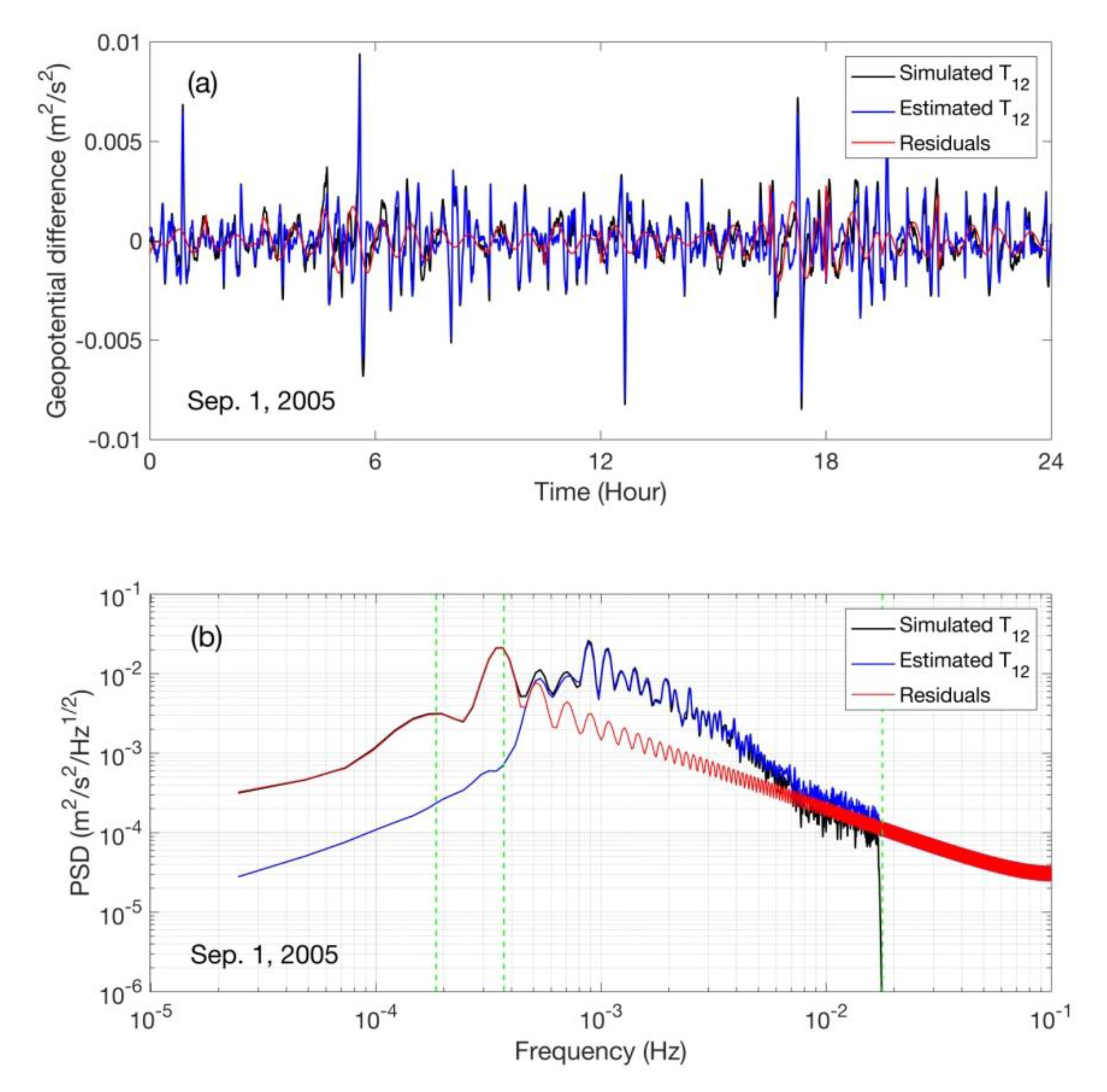
3. Geopotential Differences Estimation Based on the RCR Technique

The geopotential difference T 12 in Equation (7) due to surface mass changes can be obtained after the static geopotential and other high-frequency time-variable gravitational potential (listed in Table 1) are removed based on the energy balance Equation (2). However, the derived residual geopotential differences are contaminated by systematic errors, which are mainly caused by the KBR instrument and orbit errors [41,57,58], as well as the background model errors [39,59].
Because the orbit and background models used in Equation (2) are critical inputs, how to reduce the influences of orbit and background model errors is a key issue for precise estimation of geopotential differences. In this study, we treated the GNV1B orbit data as pseudo observations, and estimated purely dynamic orbits based on the dynamic integral approach. With the background models listed in Table 1, the dynamic orbits of two GRACE satellites were independently integrated every day. Meanwhile, the accelerometer data were simultaneously calibrated with respect to purely dynamic orbits. For each satellite, the estimated parameters include the initial state vectors (three positions and three velocities) and the accelerometer parameters (three biases and three scales in the three directions). When the purely dynamic orbits computed from the known background models were used as the input for energy integral Equation (2), the output geopotential differences would only contain time-variable gravity information contributed from the KBR range-rate measurements. The above similar technique had been used in previous studies on GRACE, such as Shang et al. [39], Zhao et al. [59], and Liu et al. [60].
In order to reduce systematic errors, especially at the low-frequency band (mainly due to KBR instrument errors), empirical parameters (i.e., bias, drift, and periodic components) are widely employed as follows [38,41]:
Δ T 12 = p 0 + p 1 t + p 2 c o s ( 2 π t T r e v ) + p 3 sin ( 2 π t T r e v ) + p 4 c o s ( 4 π t T r e v ) + p 5 s i n ( 4 π t T r e v ) ,
where Δ T 12 are the systematic errors; T r e v is the revolution period (~5400 s); p 0 , p 1 , p 2 , p 3 , p 4 , and p 5 are empirical parameters to be estimated, in which p 0 contains integration constant and system bias error, p 1 accounts for the drift error, p 2 and p 3 absorb the 1 CPR systematic errors, while p 4 and p 5 absorb the 2 CPR systematic errors. The parameters p 0 , p 1 , p 2 , and p 3 are estimated for every revolution, while p 4 and p 5 are estimated for every half revolution.
Unfortunately, the above empirical parameters used for mitigating systematic errors may absorb part of the temporal gravity signals as well, especially for the long-wavelength components [37,39,41,43]. In order to show the weakening effects of empirical parameters on temporal gravity signals, we did a simulation experiment as follows: First, 1 day of GRACE Level-1B data (e.g., 1 September 2005) were used to compute geopotential differences, and then the systematic errors were estimated through the empirical Equation (14); second, simulated geopotential differences (as the true values) for the day of 1 September 2005 were calculated using CSR RL06 SH solutions (truncated to degree and order 96 with the GGM05C static Earth gravity field removed); third, simulated geopotential differences were added with systematic errors that were estimated in the first step, then the above sum values were used to estimate the systematic errors again by using the empirical Equation (14), and the final estimated geopotential differences were obtained by subtracting the re-estimated systematic errors from the sum values. The two panels of Figure 1 show the (a) time series and (b) power spectral density (PSD) of the simulated geopotential difference using the CSR RL06 SH solutions (black solid curves), estimated geopotential difference using empirical parameters (blue solid curves), and geopotential difference residuals (red solid curves) for the day of 1 September 2005.
As shown in Figure 1a, compared with simulated geopotential differences, the variation ranges of the estimated geopotential difference time series are notably decreased, and the RMS of geopotential differences is reduced from 0.0015 to 0.0013 m2/s2, which means that about 13% of the geopotential difference signals were absorbed by the empirical parameters. In addition, the residuals time series is characterized by mostly low-frequency variations (due to the empirical parameters), and the influence of geopotential difference residuals cannot be ignored. From Figure 1b, we can see that the PSD of the estimated geopotential differences is decreased in the low-frequency band (especially at 1 CPR and 2 CPR), suggesting that the weakening effects of empirical parameters are mainly on long-wavelength temporal signals. It should be noted that, compared with the PSD of estimated geopotential differences, obvious decreases are observed in the simulated geopotential differences at the high-frequency band (up to 96 CPR). This is because the truncated CSR RL06 SH solutions up to the degree and order 96 were used for computing the simulated geopotential differences, which do not contain high-frequency temporal gravity signals.
In order to extract precise geopotential differences, and with the aim to preserve both the low- and high-frequency temporal gravity signals, the RCR technique was employed during the estimation of geopotential differences. In the present study, geopotential differences were computed in the following three steps. Firstly, the reference geopotential difference T 12 r e f was calculated by using CSR RL06 SH solutions up to the degree and order 50 (corresponding to a 400-km spatial resolution), in which the C20 coefficients were replaced by SLR solutions, and then T 12 r e f was removed from the geopotential difference T 12 that was computed based on the energy balance Equation (2). Secondly, through the empirical parameters fitting (EPF) using Equation (14), the systematic errors were estimated by using Δ T 12 R C R = EPF [ T 12 T 12 r e f ] , and the corrected geopotential difference was obtained by ( T 12 T 12 r e f ) Δ T 12 R C R . Thirdly, the reference geopotential difference T 12 r e f was added back to the corrected geopotential difference ( T 12 T 12 r e f ) Δ T 12 R C R , and the final estimated geopotential difference was T 12 Δ T 12 R C R .
Compared with the RCR technique, the traditional method for estimating the systematic errors is Δ T 12 = EPF [ T 12 ] , and the estimated geopotential difference is T 12 Δ T 12 . In order to illustrate the improvement of the RCR technique for estimation of the geopotential differences, Figure 2a,b show the global map of geopotential differences estimated by the traditional method and RCR technique for the month of September 2005 with the GGM05C static earth gravity field removed. Figure 2c shows the geopotential difference residuals obtained by subtracting estimates of the traditional method from those of the RCR technique. It can be seen from Figure 2a,b that geopotential differences are the direct reflections of surface mass changes, and signals estimated based on the RCR technique are obviously stronger than those of the traditional method in South America, Antarctic Peninsula, southern Africa, and Australia. However, there are also some regions with weakened signals, such as eastern Asia and North Atlantic. The RMS of geopotential differences (outliers are removed according to a 3-sigma rule) estimated by the traditional method and RCR technique are ~0.0022 and 0.0025 m2/s2, respectively. Figure 2c shows that geopotential difference residuals are mainly characterized by low-frequency gravity signals, which are absorbed by the empirical parameters used in the traditional method. Therefore, the RCR technique is helpful to retain the low-frequency gravity signals, and the inversion of surface mass variations at a full spectrum (both low and high frequency) can be obtained.

4. Results

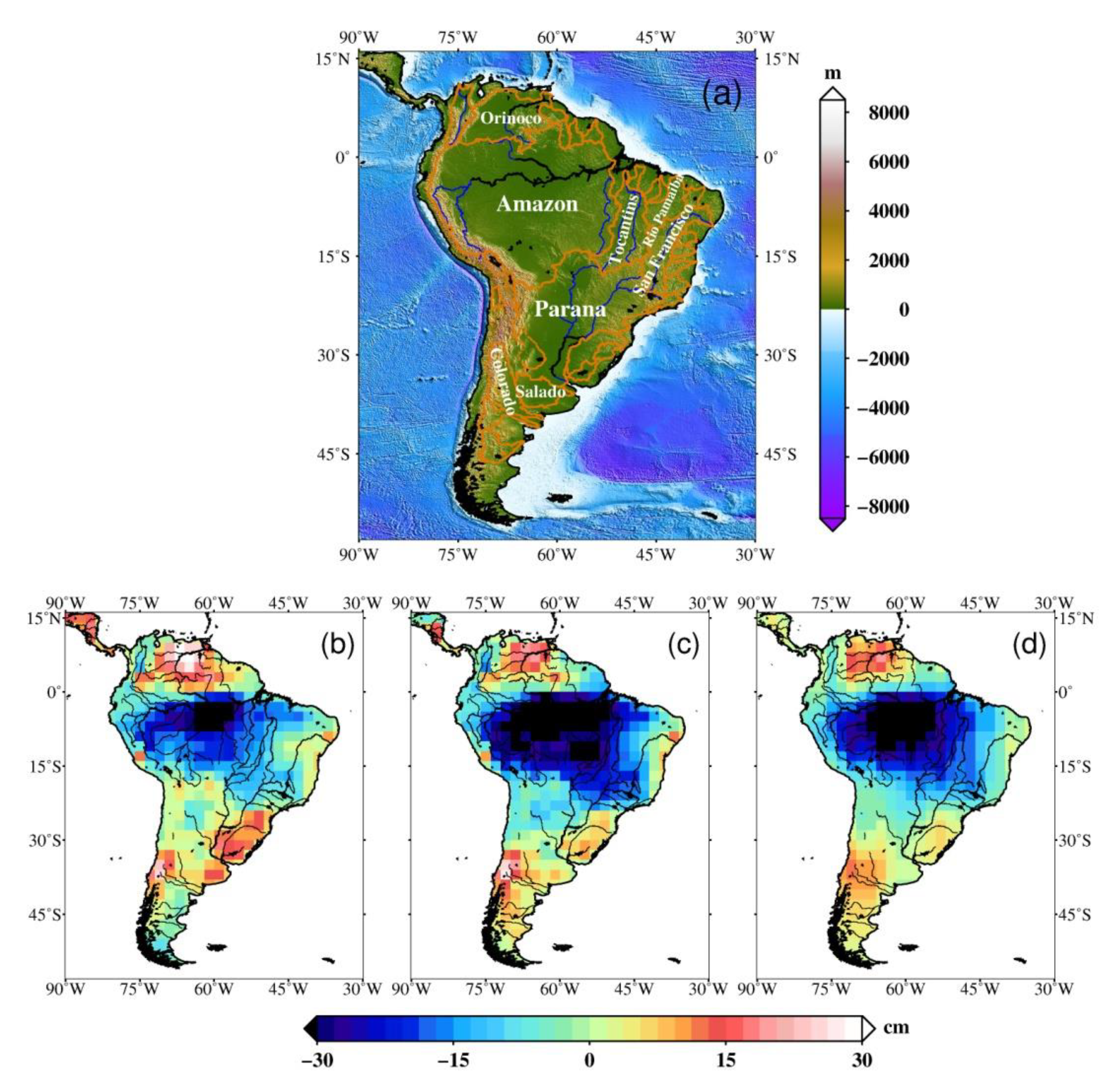
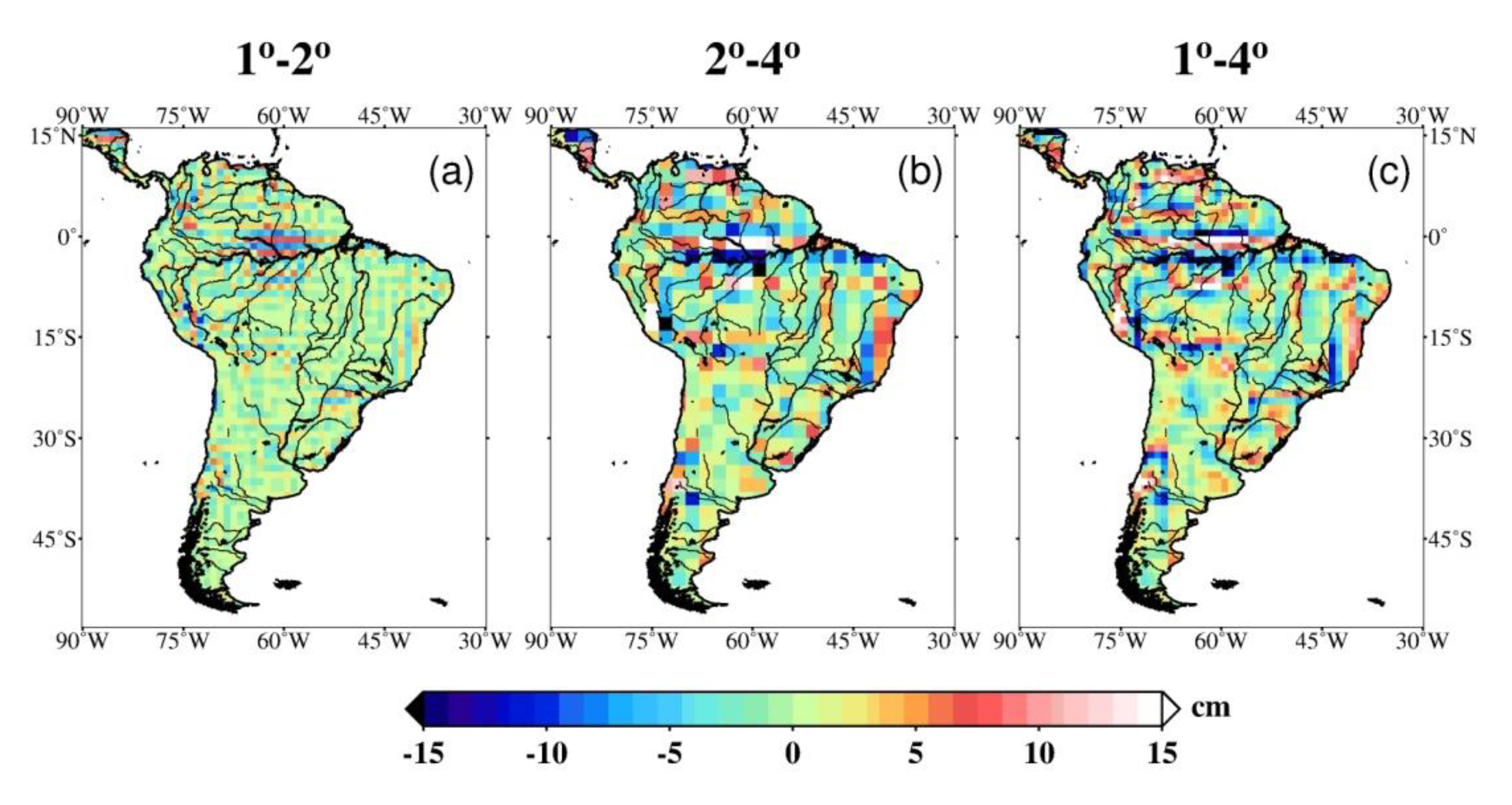
4.1. Preliminary Tests over South America

In order to verify the proposed method (and software), regional surface mass variations on 2° × 2° geographic grids over South America ([60°S–15°N, 90°W–30°W], see Figure 3a) were inverted from geopotential difference estimates in September 2005, and GLDAS-derived TWS changes were employed as a priori constraints to reduce the ill condition in regional mass estimations from GRACE. In this study, the optimal regularization parameters were determined based on the iterative least-squares estimation method. Specifically, we set initial values α = 1 and σ y 2 = 0.002 m2/s2 in Equation (10), and took the maximum value of EWH differences between two adjacent iterations to be less than 10−6 mm as the convergence condition. The final estimated mass variations can be obtained after about 10 iterations. Figure 3b,c show the regional surface mass variations over South America inverted from geopotential differences estimated by the traditional method and RCR technique in September 2005, respectively. Figure 3d presents the corresponding surface mass variations over South America derived from the CSR RL06 SH solutions with 300-km Gaussian smoothing and P3M6 decorrelation filtering for comparisons.
As shown in Figure 3, there are obvious differences in regional surface mass variations inverted from geopotential differences estimated by the traditional method and RCR technique. The mass variations over Amazon basin show substantially stronger negative anomalies in Figure 3c than in Figure 3b, while the mass variations over Orinoco basin (in the north), western part of Parana basin, and parts of southern South America (e.g., in Uruguay) show stronger positive anomalies in Figure 3b than in Figure 3c. However, compared with surface mass variations inverted from geopotential differences estimated by the traditional method, the results from geopotential differences estimated by the RCR technique are more consistent with CSR RL06 SH solutions. Moreover, mass variation signals in Figure 3c,d are stronger than those in Figure 3b, and the RMS of mass variations in Figure 3b–d are 13.7, 18.4, and 16.7 cm, respectively. The reason, as mentioned before, is that the empirical parameters used in the traditional method absorbed the long-wavelength gravity signals, and thus weakened the mass variation estimates. In addition, the signals of mass variations in Figure 3c are stronger than those in Figure 3d, which strongly suggests that the regional mascon solutions can retain more signal energy and enhance regional mass variation inversion.
To assess the effects of different block sizes on the inversion results, Figure 4 shows regional mass variations estimated on 1° × 1° grids, 2° × 2° grids, and 4° × 4° grids from geopotential differences computed by the RCR technique in September 2005 using GLDAS-derived TWS changes as a priori constraints, and the corresponding residuals between geopotential difference-estimated mass variations and GLDAS-derived TWS changes are also presented. Figure 5 shows the residuals between regional mass variations estimated on different mascon block sizes.
As shown in Figure 4, although the a priori information from GLDAS TWS changes can contribute to the final estimated mass variations, there are obvious differences between regional mass variation solutions and GLDAS-derived TWS changes, no matter what sizes of grids were used for the estimation. The residuals can be considered as the new contributions from GRACE observations to the final estimated regional mass variations, and the added value from GRACE data can obviously enhance the signals of mass variations over South America, especially in basins of Amazon, Orinoco, and Colorado, etc. Small mascon block sizes are expected to help to improve the level of details in estimated mass variations (e.g., from 4° × 4° to 2° × 2° grids), but there are no notable changes of signal amplitudes by decreasing the size of the mascon blocks, and no gains of details in our experiments (see Figure 4a–c). In addition, we can draw a similar conclusion from Figure 5 based on the residuals between regional mass variations estimated on different mascon block sizes. The RMS differences of the inversion results between 1° × 1° and 2° × 2° grids, 1° × 1° and 4° × 4° grids, 2 × 2° and 4° × 4° grids are ~1.6, 3.3, and 3.1 cm, respectively. Considering the intrinsic optimal spatial resolution of the GRACE data is limited at ~200–300 km, and the 1° × 1° regional mascon solution will have leakage errors, while the 2° × 2° grids computation seem enough to represent the GRACE resolution.

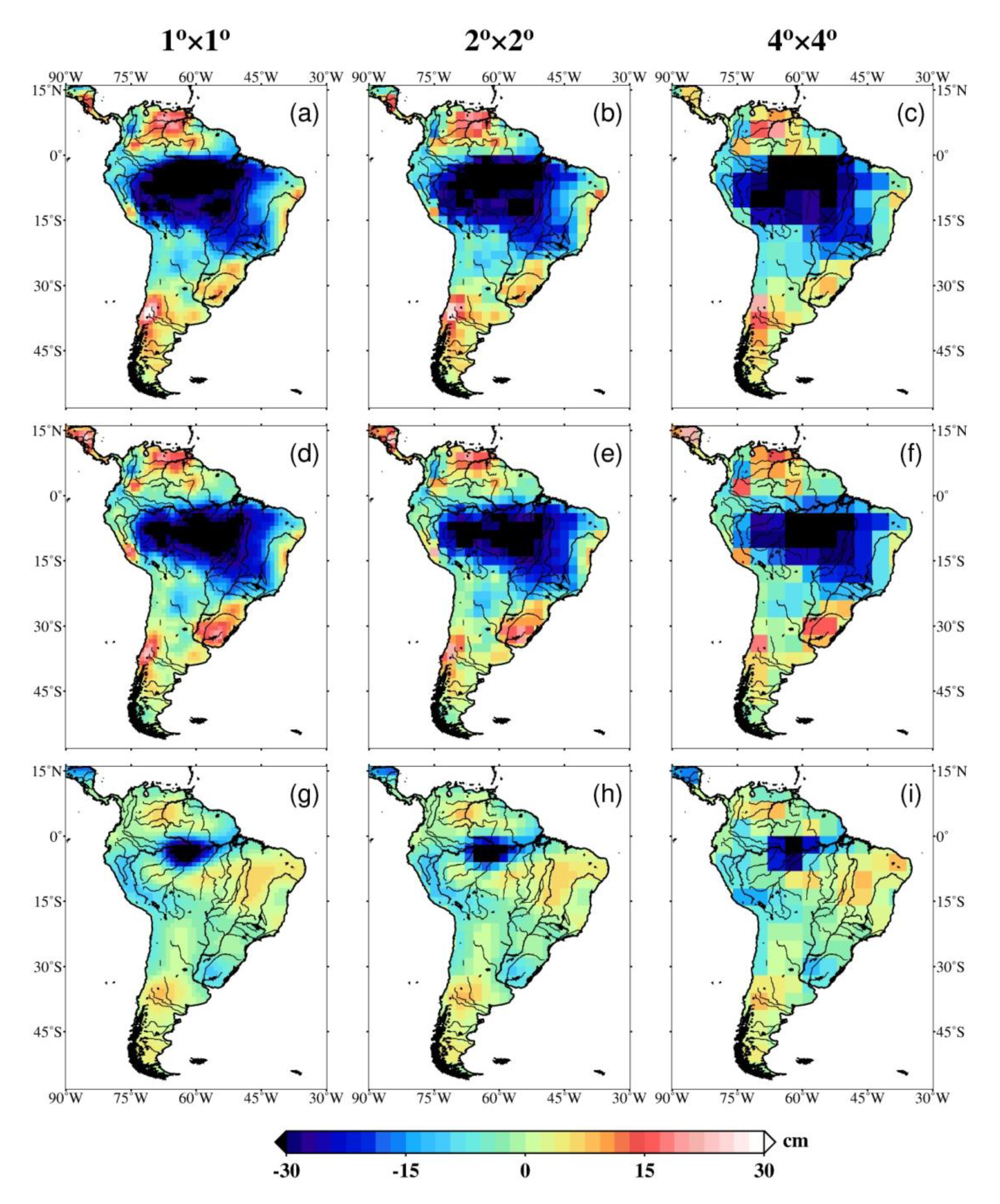
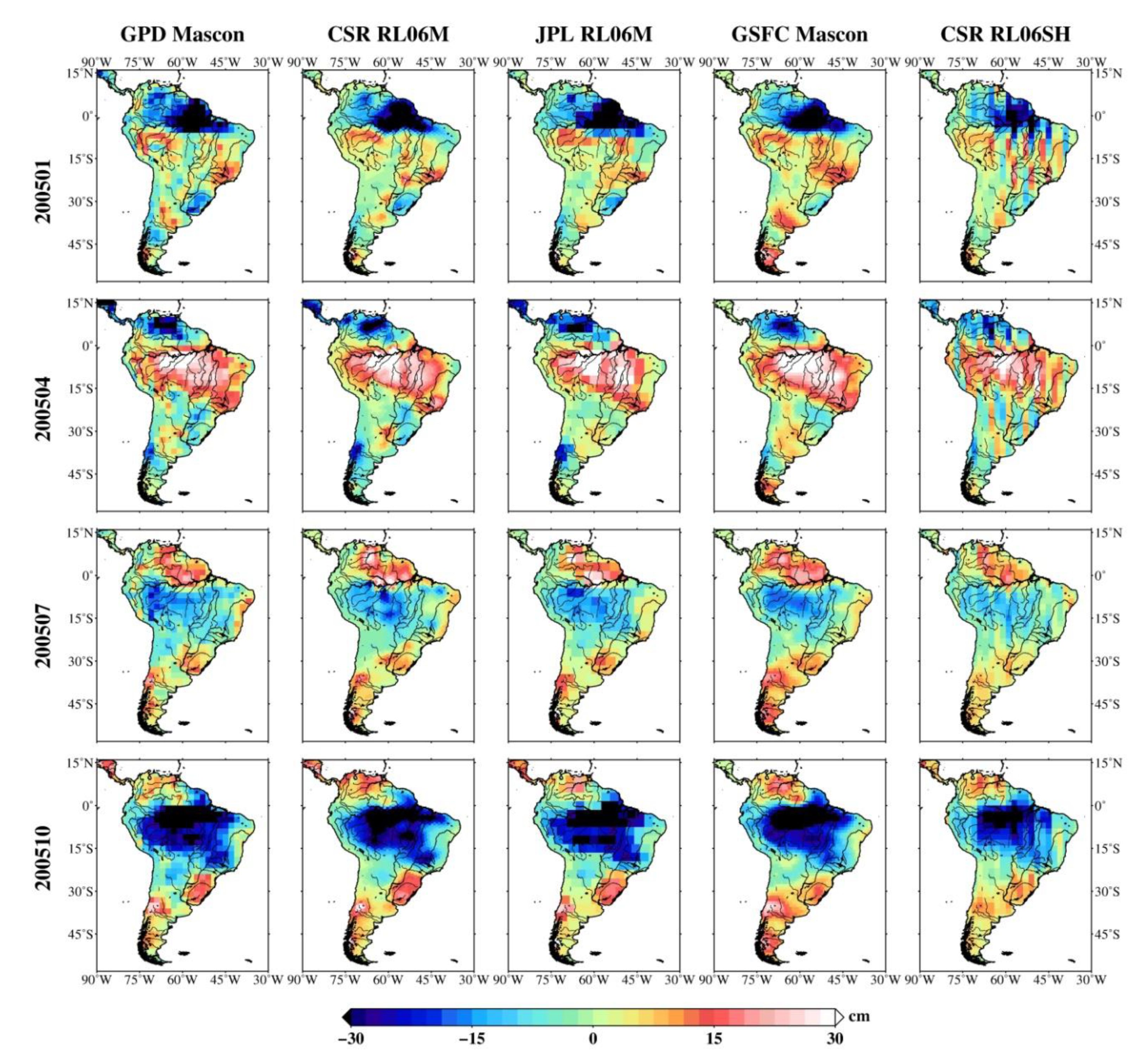
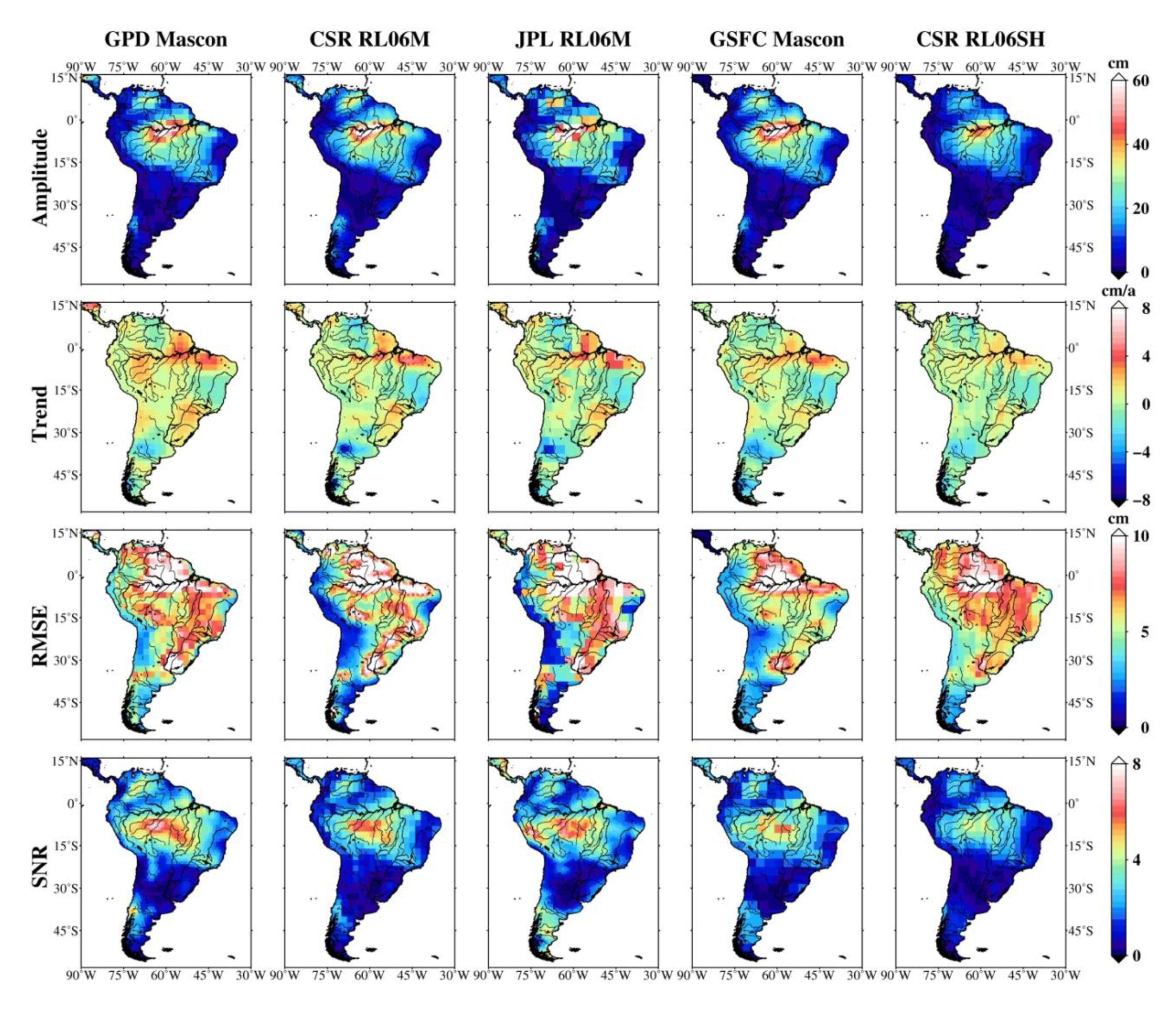
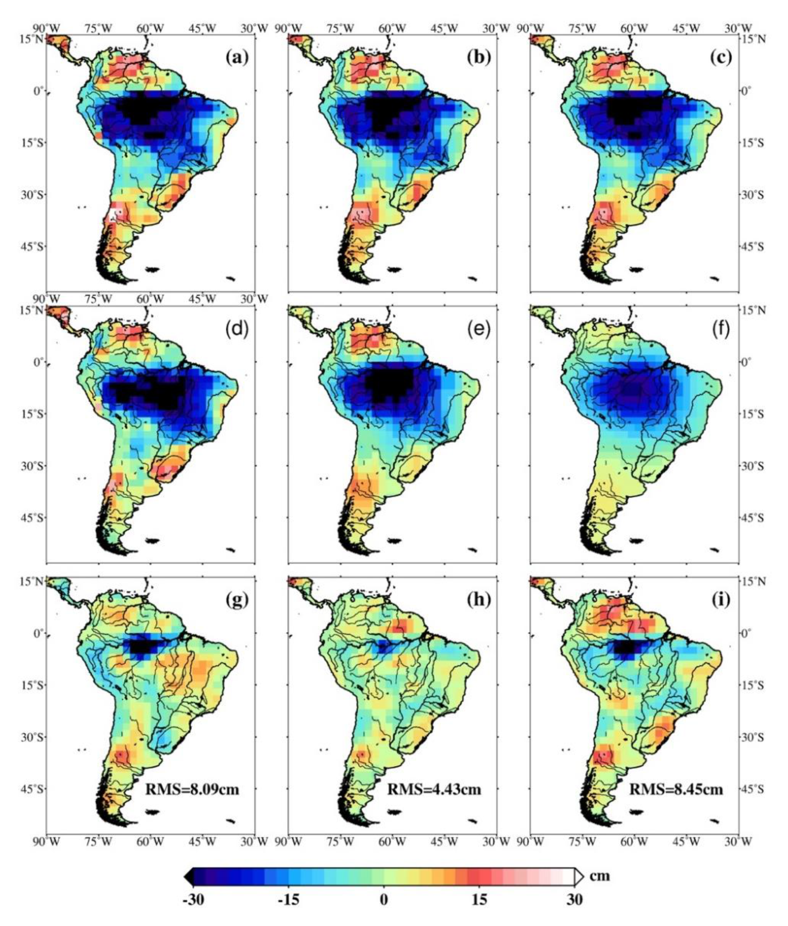
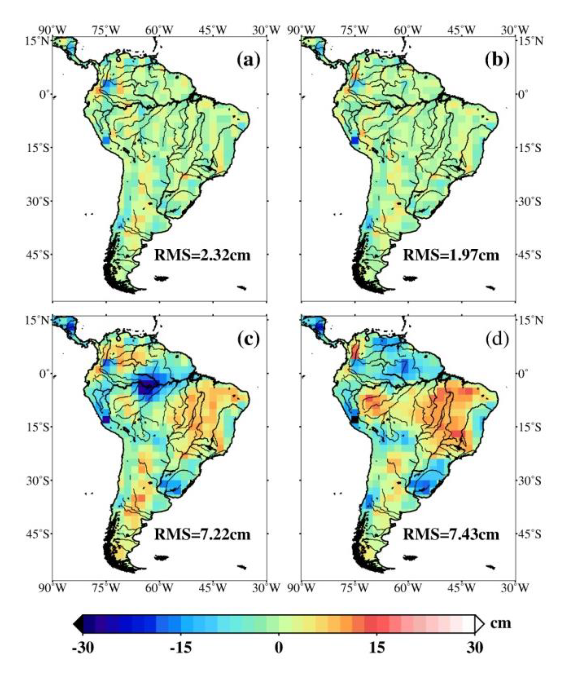
4.2. Spatial Distribution of Mass Changes over South America

To examine the performance of regional mass variations inverted from GRACE intersatellite geopotential differences, we employed the GRACE Level-1B RL03 data from January 2005 to December 2010 to calculate the precise geopotential differences based on the RCR technique, and estimated regional surface mass variations on 2° × 2°grids at monthly intervals over South America. We then compared the results with the official GRACE RL06 mascon solutions and SH solutions. It should be noted that all the mascon solutions and SH solutions had been applied with the corrections as mentioned in Section 2.4.4 (i.e., the C20 term replacement, the geocenter correction, and the GIA correction, unless otherwise mentioned). Figure 6 shows the spatial distributions of regional mass variations over South America in January (the first row), April (the second row), July (the third row), and October (the fourth row) 2005 from “the new” geopotential difference-based regional mascon solutions (hereinafter called GPD Mascon, the first column), CSR RL06 mascon solutions (CSR RL06M, the second column), JPL RL06 mascon solutions (JPL RL06M, the third column), GSFC mascon solutions (GSFC Mascon, the fourth column), and CSR RL06 SH solutions (CSR RL06SH, the fifth column), respectively.
As shown in Figure 6, both of the mascon solutions and the SH solutions can reflect the same spatial distribution characteristics of surface mass variations over South America in the four selected months. However, due to the spatial filtering in post-processing of GRACE SH solutions, the amplitudes of surface mass variations from CSR RL06SH are obviously smaller than those of the four mascon solutions. Moreover, there are apparent residual longitudinal stripes in CSR RL06SH (especially in January and April 2005), although the post-processing was applied to these SH solutions. The reason is that, unlike the mascon solutions, the GRACE SH solutions are solved without using any constraints or a priori information.
Comparing the four mascon solutions in Figure 6, we can see that all the mascon solutions reveal similar main characteristics of the mass changes over South America in the selected four months, but the details of the mass variations from the four mascons are different. For instance, as can be seen from the mass variations in January 2005, there are apparent positive anomalies in the Salado basin in GPD Mascon and GSFC Mascon, while these details are not obvious in CSR RL06M and JPL RL06M. For July 2005, the mass change signals of CSR RL06M and JPL RL06M are slightly stronger than those of GPD Mascon and GSFC Mascon in the Orinoco basin and the north of Amazon basin. From the four mascon solutions shown in April and October 2005, the strongest mass variations signals are mainly in the Amazon and Tocantins basins, and the distribution of mass variations over South America in April 2005 shows almost an inverse pattern compared with that in October 2005.
In addition, RMS differences between GPD Mascon and CSR RL06M, GPD Mascon and JPL RL06M, and GPD Mascon and GSFC Mascon for the four months in 2005 are listed in Table 2, and the ranges of RMS differences between the three official mascon solutions are also presented for comparisons. These results show that GPD Mascon appears closer to GSCF Mascon but differs much more from JPL RL06M. For example, the RMS differences between the GPD Mascon and CSR RL06M, GPD Mascon and JPL RL06M, and GPD Mascon and GSFC Mascon in April and October 2005 are 6.18 vs. 6.72 cm, 7.25 vs. 7.93 cm, and 5.42 vs. 5.46 cm, respectively. Meanwhile, differences among CSR RL06M, JPL RL06M, and GSCF Mascon are also obvious, e.g., the ranges of RMS differences between the three official mascon solutions are 5.87–6.75 cm in April 2005, and 5.67–6.70 cm in October 2005, respectively.
In order to better understand the surface mass variations inferred from different solutions over South America, a simultaneous fit of annual, semi-annual, trend, and bias was made to the time series for each mascon block of the above five solutions (i.e., GPD Mascon, CSR RL06M, JPL RL06M, GSFC Mascon, and CSR RL06SH). Figure 7 shows the spatial distributions of annual amplitudes (the first row), trends (the second row), root-mean-square error (RMSE, the third row), and signal-to-noise ratio (SNR, the fourth row) of mass variations over South America (over the period January 2005 to December 2010) derived from the five solutions, respectively.
As shown in Figure 7, the spatial patterns of the annual amplitudes and trends for the five solutions are consistent with each other, but the differences between each other can still be observed if we carefully examine these results at basin scale. An apparent observation is that annual amplitudes and trends over the Amazon basin are significantly larger in the four mascon solutions as compared to those from the CSR RL06SH results. Because the four mascon solutions are provided on different sizes of grids (not the real spatial resolutions), for better comparisons, we resampled the GPD Mascon, JPL RL06M, and GSFC Mascon into 0.25° × 0.25° grids, consistent with the CSR RL06M grid’s resolution. In terms of annual amplitudes, the correlation coefficients between GPD Mascon and the three other mascons (CSR RL06M, JPL RL06M, and GSFC Mascon) are ~0.95, 0.93, and 0.97, respectively. In terms of trends, the corresponding correlation coefficients are ~0.85, 0.79, and 0.88, respectively. The relatively lower correlation coefficients for the trends are attributed to the fact that temporal mass variations in South America are dominated by seasonal hydrological signals, and the long-term trend is usually small, and its uncertainty is relatively larger. Nevertheless, our results demonstrate that regional mass variations inverted from geopotential differences estimated by the RCR technique are comparable to those from the official GRACE mascon solutions, without using low degrees of SH solutions to complement the missing long-wavelength signal (unlike in the studies, e.g., Frédéric Frappart et al. [43] and Ramillien et al. [44]).
In addition, the RMSE of mass variation residuals and SNR were used to evaluate the errors and accuracies of different solutions. As mentioned above, a simultaneous fit was made to the time series for each mascon block, and mass variation residuals were obtained by removing the fitted signals from the mass change time series. Then, the residual RMSE for each block was estimated, and the SNR was computed as the quotient between the annual amplitude and RMSE. As can be seen from Figure 7, the RMSE patterns from the five solutions are similar in most of the regions. For example, the mean RMSEs in the Amazon basin are ~4.23, 4.24, 4.46, 4.11, and 3.34 cm for GPD Mascon, CSR RL06M, JPL RL06M, GSFC Mascon, and CSR RL06SH, respectively. Here, due to the spatial smoothing and filtering applied to the SH solutions, the mean RMSEs from CSR RL06SH in the Amazon basin are the smallest (compared with those of the mascon solutions). The SNR patterns from the five solutions are similar to those of the annual amplitudes shown in the top row of Figure 7. The mean SNR in the Amazon basin are ~4.65, 4.55, 4.56, 4.90, and 4.51 for GPD Mascon, CSR RL06M, JPL RL06M, GSFC Mascon, and CSR RL06SH, respectively. Again, these comparisons also suggest that the GPD Mascon solutions are comparable to the official GRACE mascons, and further demonstrate the effectiveness of solving regional mascon solutions using geopotential differences estimated by the RCR technique with a priori constraints.

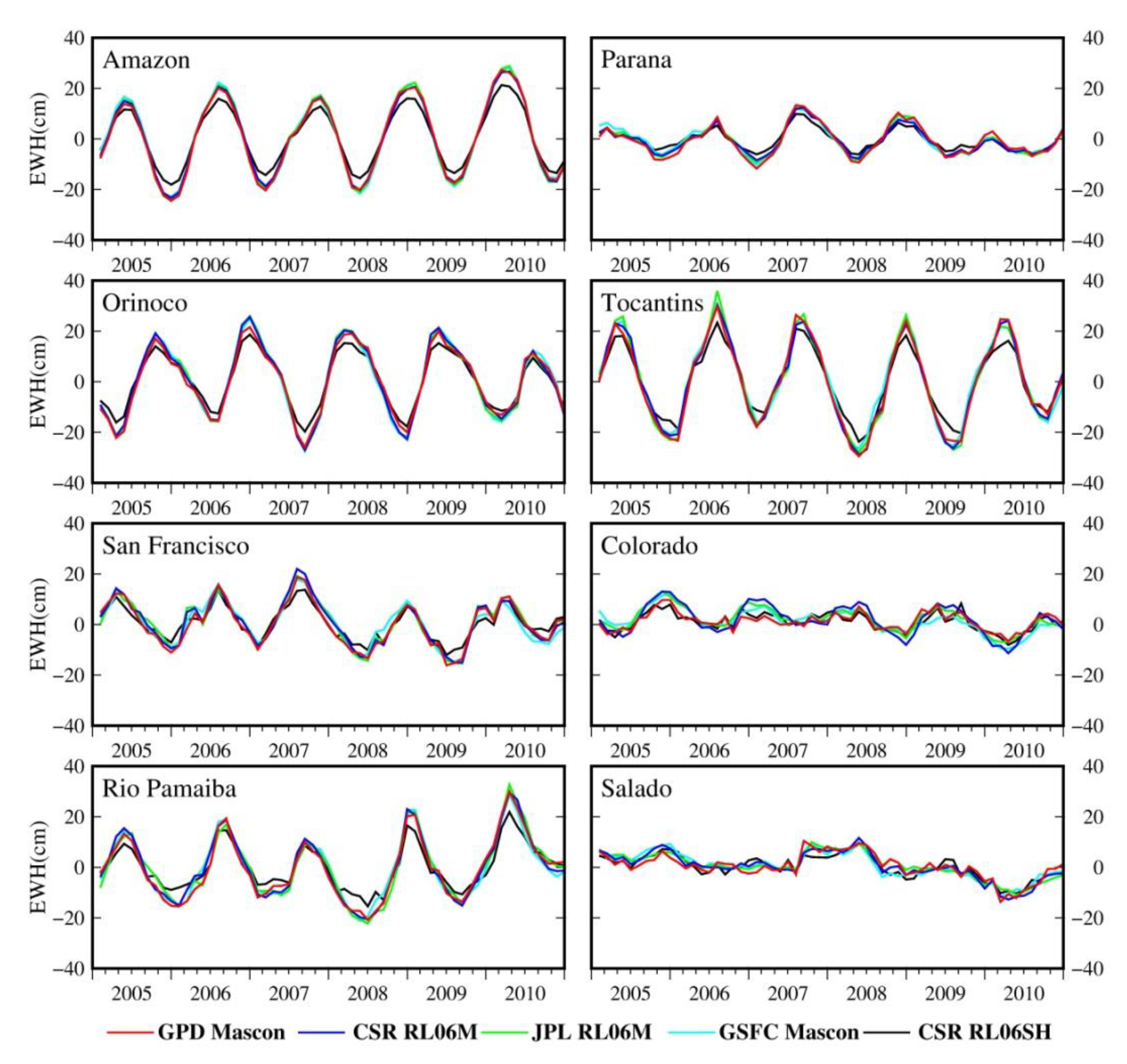
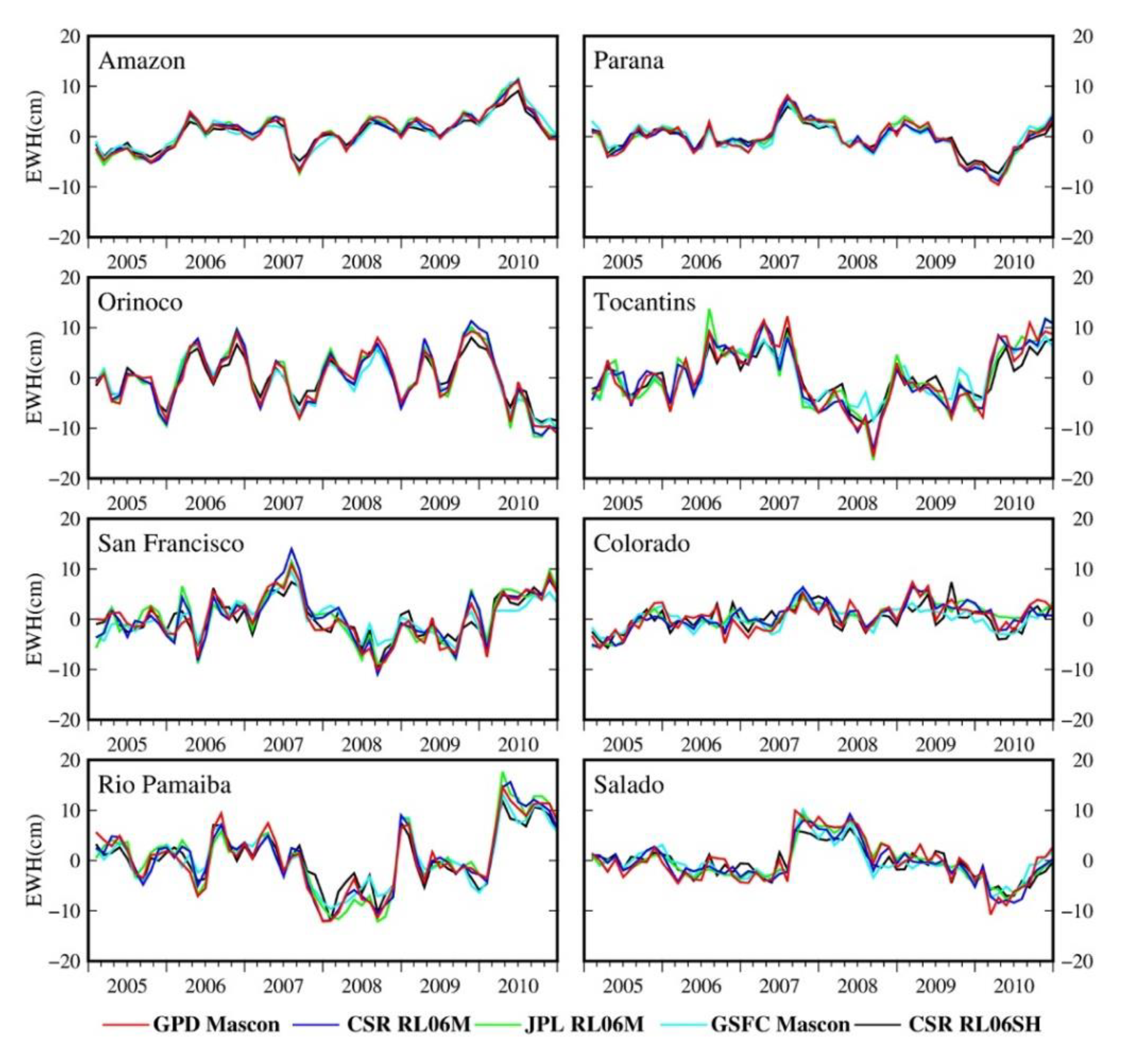
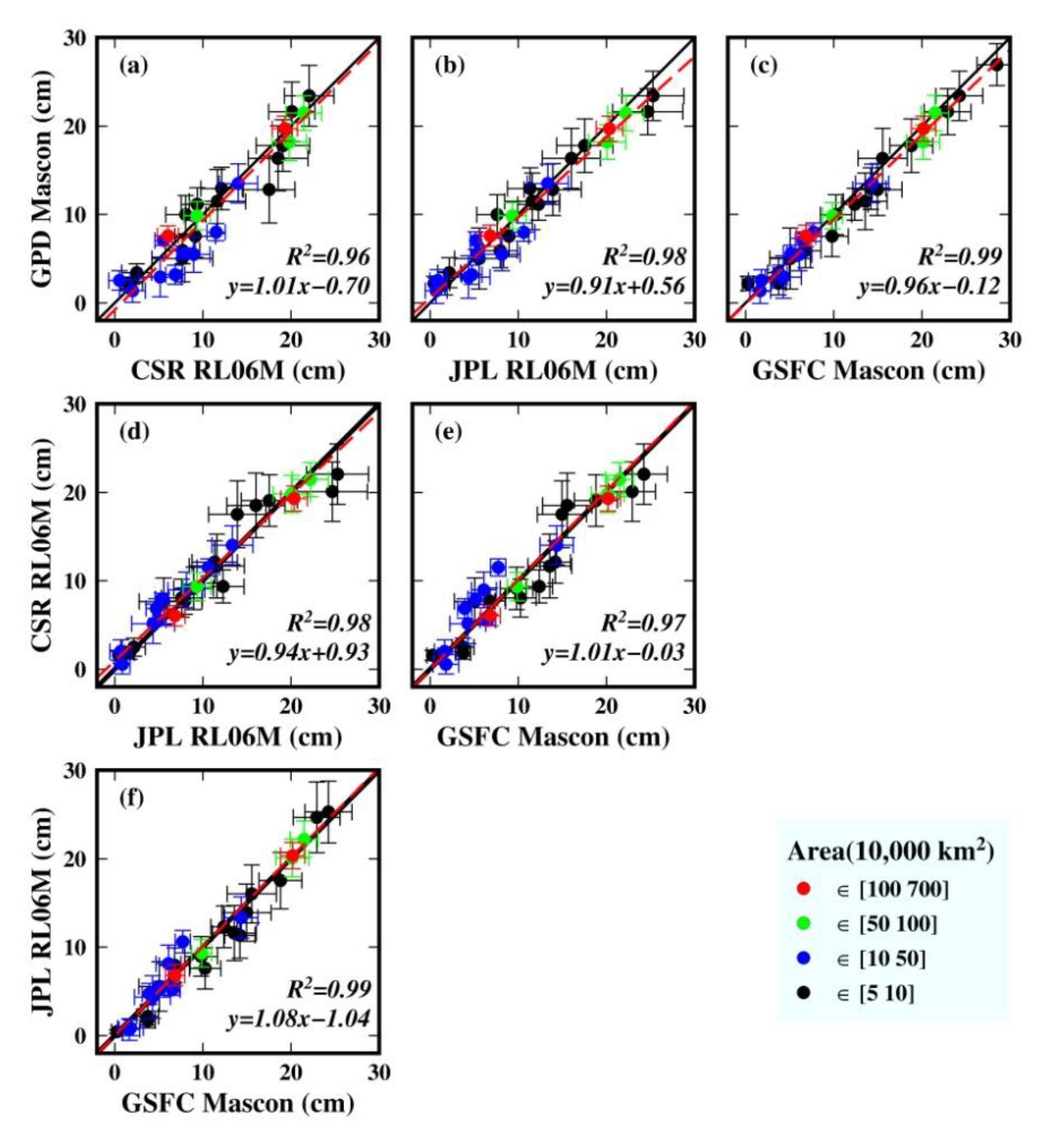
4.3. Basin-Scale Mass Changes over South America

In order to compare surface mass variations derived from different solutions over South America at the basin scale, mass variations over the eight largest basins (i.e., Amazon, Parana, Orinoco, Tocantins, San Francisco, Colorado, Rio Pamaiba, and Salado, see Figure 3a) were further analyzed. Figure 8 shows mass change time series for the eight basins over the period January 2005 to December 2010, derived from GPD Mascon, CSR RL06M, JPL RL06M, GSFC Mascon, and CSR RL06SH, respectively. Figure 9 presents the non-seasonal mass change time series for the eight basins, which were obtained by removing seasonal signals and long-term trends from the time series shown in Figure 8. Table 3 lists the corresponding annual amplitudes and trends of surface mass change time series for these eight basins, and the uncertainties correspond to a 95% confidence interval.
As can be seen from Figure 8, basin mass change time series from the five solutions (i.e., GPD Mascon, CSR RL06M, JPL RL06M, GSFC Mascon, and CSR RL06SH) agree well with each other, especially for the large river basins with stronger seasonal signals (e.g., in Amazon, Parana, and Orinoco). However, discrepancies are also obvious, especially in some small basins with weaker mass change signals (e.g., in Colorado and Salado). This is because the uncertainty estimated in small basins with weaker mass change signals is relatively large compared to mass change signals themselves. In addition, due to the spatial filtering applied to the SH solutions, mass change signals from CSR RL06SH over the eight basins are slightly smaller than those of the mascon solutions (which can also be found in Table 3).
As listed in Table 3, the annual amplitudes for the four mascon solutions agree well, especially in basins with stronger mass change signals (e.g., the Amazon, Parana, Orinoco, Tocantins, San Francisco, and Rio Pamaiba), and the differences of annual amplitudes are acceptable as compared to their uncertainties. Aside from the seasonal variability, basin-scale non-seasonal signals affected by extreme climate events, such as floods and droughts, are also of great interest. Figure 9 shows that the non-seasonal signals of the four mascon solutions for the eight basins are also consistent. For instance, in the case of the Amazon basin, the correlation coefficients of mass change time series between the four mascon solutions all reach up to 0.99. With the seasonal signals and linear trends removed, the correlation coefficients of mass change time series between GPD Mascon and the other three mascons (CSR RL06M, JPL RL06M, and GSFC Mascon) still reach up to 0.99, 0.98, and 0.97, respectively. In the Salado basin (the smallest of the eight basins), after removing the seasonal signals and linear trends, the correlation coefficients of mass change time series between GPD Mascon and CSR RL06M, JPL RL06M, and GSFC Mascon are ~0.91, 0.91, and 0.86, respectively. The excellent consistency among basin-scale mass changes from the four mascon solutions indicate that all these four mascon solutions perform fairly well at both seasonal and non-seasonal time scales.
The linear trends of the mass changes over the eight basins are small, and there are obvious differences between the estimated trends from these five different solutions (see Table 3). Moreover, the uncertainties for the estimated trends are relatively larger, and in some cases the estimated uncertainty is even greater than the trend itself. The obvious differences in trends can also be confirmed from the lower spatial correlation of trends as analyzed in Section 4.2 (see Figure 7). As mentioned before, basin-scale mass variations over South America are dominated by seasonal TWS changes, and trends are usually small and uncertainties are relatively larger, leading to poorer agreements in trends.
In order to further analyze the consistency among the four mascon solutions, a total of 30 river basins (with areas larger than 50,000 km2) over South America were selected for comparisons. Mass change time series of the basin average for the 30 basins over the period January 2005 to December 2010 were calculated, and simultaneous fits of seasonal terms and trends (mentioned in Section 4.2) were made to these time series. Figure 10 shows the scatterplot of annual amplitudes for the 30 river basins over South America obtained by comparing the four mascon solutions with each other, i.e., (a) GPD Mascon vs. CSR RL06M, (b) GPD Mascon vs. JPL RL06M, (c) GPD Mascon vs. GSFC Mascon, (d) CSR RL06M vs. JPL RL06M, (e) CSR RL06M vs. GSFC Mascon, and (f) JPL RL06M vs. GSFC Mascon over the period January 2005 to December 2010.
As shown in Figure 10, if the two mascon solutions in one panel agree perfectly, the filled cycle would align on the y = x line (black solid lines). However, if the scattered points for any two mascon solutions are distributed around that line, the corresponding fitting curve is the linear regression equation y = kx + b (given by the red dashed line), and the relative positions of the black solid line and the red dashed line can describe the consistency of annual amplitudes between the corresponding two solutions. We can see that for every panel in Figure 10, the red dashed lines are very close to the black solid lines and the correlation coefficients are all greater than 0.96, which indicate that the consistencies of annual amplitudes for the four mascon solutions are very good, even though notable differences can also be observed.
In general, when the slope of the red dashed line is less than 1.0, the y-axis values are smaller than those of the x-axis, e.g., GPD Mascon vs. JPL RL06M, GPD Mascon vs. GSFC Mascon, and CSR RL06M vs. JPL RL06M, as shown in Figure 10b–d, and vice versa from those in Figure 10a,e,f. In a particular case of GPD Mascon vs. CSR RL06M (Figure 10a), although the slope is greater than 1.0, the red dashed line is generally below the solid black line. In the sense of statistics, it means that the annual amplitudes of the 30 basins from GPD Mascon are slightly smaller than those from CSR RL06M. The relatively larger discrepancies in small basins among the four mascon solutions appear to be the main reason affecting the consistency.

5. Discussion

This study focused on applying the improved method to estimate regional mascon solutions using GRACE intersatellite geopotential differences, and the inversion results were examined through comprehensive comparisons with the official GRACE mascon solutions. A proper validation was not carried out through the use of independent in situ data. However, the comparative analysis shows that our geopotential difference-based regional mascon solutions (GPD Mascon) are comparable to the three official GRACE mascon solutions at the basin scale (i.e., the accuracies of these four mascon solutions are very similar), and have demonstrated the feasibility and effectiveness (and advantage) of the proposed method.
As can be seen from the comparative analysis, the spatial patterns and characteristics of mass variations over South America from GPD Mascon agree well with those from the three official GRACE mascon solutions (see Figure 6 and Figure 7), and the annual amplitudes of mass change time series from the four mascon solutions at the basin scale over South America show good consistency with each other (see Table 3 and Figure 10), and the non-seasonal signals from these four mascon solutions in larger basins are also in good agreement with each other (see Figure 9). However, notable differences among the four mascon solutions still exist, in particular at the basin scale. The reasons for this are twofold. Firstly, the mass variations inversion methods are different, i.e., all the official GRACE mascon solutions are directly solved from instrument observations based on the dynamic method, while the GPD Mascon solutions are computed from intermediate observations (i.e., intersatellite geopotential differences), which are estimated based on the energy balance approach. Therefore, different approximate errors in inversion models will lead to differences in the final estimated mass variations. Secondly, different processing strategies (e.g., regularization constraints, background models, sizes of mascon blocks, and data pre-processing, etc.) can also induce discrepancies between these mascon inversion results. For instance, even though the three official GRACE mascon solutions are all solved by the dynamic method, differences among them are also obvious. The main reason accounting for this includes the different regularization constraints and different sizes of mascon blocks for the three mascon solutions as introduced in Section 2.4.3.
In our case study, surface mass changes over South America are dominated by seasonal hydrological signals, thus TWS changes from hydrological models (i.e., GLDAS) are chosen as a priori information for the estimation of mascon solutions. As mentioned in Section 4.1, the a priori information from GLDAS-derived TWS changes can contribute to the final estimated mascon solutions, but how the a priori constraints can affect the output needs to be assessed. It is well known that hydrological models suffer from large uncertainties in regions that have poor-quality data (e.g., in high-mountain Asia), or even no data (e.g., in Greenland and Antarctic) [61,62,63]. Therefore, it is necessary to analyze the influences of different a priori information on the estimation of mascon solutions, especially if only the rough a priori information can be obtained. To assess the effects of different a priori constraints on the inversion results, we employed CSR RL06 SH solutions post-processed with different Gaussian smoothing radius as a priori models to estimate the mascons, and compared them with the previous results, which use GLDAS-derived TWS changes as a priori models. Figure 11 shows the regional mass variations estimated from geopotential differences in September 2005 by using different a priori models, and the corresponding residuals between estimated mass variations and the a priori models are presented. Figure 12 shows the corresponding residuals between the geopotential difference-estimated mascon solutions by using different a priori models, and also the residuals between the a priori models.
As shown in Figure 11a–c, there are only minor differences between the mascon solutions estimated by our improved method through using different a priori models. When taking the GLDAS-derived TWS changes, the CSR RL06 SH solution with 300-km Gaussian filtering, and the CSR RL06 SH solution with 750-km Gaussian filtering as a priori models, the RMS residuals between the estimated mass variations and the a priori models are ~8.09, 4.43, and 8.45 cm, respectively. This is true that the a priori model of CSR RL06 SH solutions with 300-km Gaussian filtering is closer to the estimated mascons. However, as shown in Figure 12, although there are obvious differences between the three a priori models (e.g., RMS residuals is larger than 7.0 cm), the estimated mascon solutions agree well with each other (e.g., RMS residuals is ~2.0 cm). This shows that our improved method can robustly estimate the mascon solutions, which are less affected by a priori information (even by using a rough a priori information). In other words, GRACE SH solution-derived TWS changes can be used as alternative a priori models when the quality of hydrological models is poor, or no a priori information can be obtained. Meanwhile, the resolution matrix [64] (i.e., ( A T A + α σ y 2 C x 1 ) 1 α σ y 2 C x 1 derived from Equation (10)) was used to analyze the relative contribution of a priori constraints to the mascon solutions. Our results show that when using GLDAS-derived TWS changes, CSR RL06 SH solutions with 300-km Gaussian filtering, and CSR RL06 SH solutions with 750-km Gaussian filtering as a priori models, the average contributions of a priori constraints to the final mascon solutions are ~11.8%, 12.9%, and 10.5%, respectively. It indicates that the contributions of a priori constraints to the mascon solutions are not dominant, and most contributions are from GRACE observations.

6. Conclusions

In this study, we presented an improved method for the estimation of regional mass variations from GRACE intersatellite geopotential differences using a priori constraints. Firstly, an alternative analytic formula was presented to incorporate the KBR range-rate into the improved energy balance equation, and precise intersatellite geopotential differences were estimated from GRACE Level-1B data based on the RCR technique, which can avoid the long-wavelength gravity signals to be absorbed by empirical parameters. Secondly, GLDAS-derived TWS changes were used as a priori constraints to reduce the ill condition for solving regional mass variations from geopotential difference data, and an adaptive algorithm was employed to determine the optimal regularization parameters based on iterative least-squares estimation. Thirdly, regional mascon solutions inverted from geopotential differences over South America on 2° × 2° grids at monthly intervals from January 2005 to December 2010 were compared to the official GRACE mascon solutions.
The results show that the regional mascon solutions inverted from geopotential differences estimated by the RCR technique using GLDAS hydrological models as a priori constraints can retain more signal energy and enhance regional mass variation inversion, and the final estimated mascon solutions are less affected by the a priori information. The spatial distribution characteristics of mass variations over South America from the geopotential difference-based regional mascon solutions (i.e., GPD Mascon) agree well with those from the three official GRACE mascon solutions (i.e., CSR RL06M, JPL RL06M, and GSFC Mascon). Additionally, the annual amplitudes of mass change time series derived from the four mascon solutions for the eight largest basins over South America show good consistencies with each other. Aside from the seasonal variability, the basin-scale non-seasonal signals from these four mascon solutions are also in good agreement with each other. However, obvious differences can be observed among the spatial patterns and trends derived from the four mascon solutions, especially in the small basins. The discrepancies are mainly due to different inversion methods with different error approximations and data processing strategies (regularization constraints, background models, sizes of mascon blocks, and data pre-processing, etc.) applied. In addition, differences in trends are also due to their small magnitudes, as mass variations over South America basins are dominated by seasonal hydrological signals. Despite the expected discrepancies, the GPD Mascon solutions are comparable to the three official mascon solutions at the basin scale, and without needing low degrees of SH solutions to complement the missing long-wavelength signal, which demonstrates the feasibility and advantage of the proposed method.
It should be noted that our GPD Mascon solutions did not account for the leakage effects across land–ocean boundaries (like the CRI filter used in JPL RL06M), which might affect the comparisons with the official GRACE mascon solutions. However, if the basin is large or far away from the ocean, the leakage effect is expected to be small. Our future work will include the implementation of leakage corrections to further improve the accuracy of geopotential difference-based regional mascon solutions. In addition, GRACE Follow-On is equipped with laser ranging interferometer (LRI), which can provide more accurate intersatellite ranging data, so we plan to use GRACE Follow-On data to further analyze and verify the geopotential difference-based method in the future.

Author Contributions

Conceptualization, B.Z. and Q.L.; Methodology, B.Z., Q.L. and Z.L.; Software, B.Z. and Q.L.; Validation, J.C., Q.L. and H.Z.; Data curation, B.Z., Q.L. and H.Z.; Funding acquisition, B.Z. and Q.L.; Writing—original draft preparation, B.Z. and Q.L.; Writing—review and editing, B.Z., J.C. and Z.L. All authors have read and agreed to the published version of the manuscript.

Funding

This research was funded by the National Key Research and Development Program of China (Grant No. 2018YFC1503503), the National Natural Science Foundation of China (Grant Nos. 41974015, 41504014, and 41474019), and the State Key Laboratory of Geo-information Engineering (No. SKLGIE2017-Z-1-2).

Acknowledgments

We are grateful to Center of Space Research (CSR) and Jet Propulsion Laboratory (JPL) for providing GRACE Level-1B data and GRACE RL06 spherical harmonic solutions and mascon solutions, Goddard Space Flight Center (GSFC) for providing GRACE mascon solutions, and Goddard Earth Sciences Data and Information Services Center (GES DISC) for providing GLDAS data. The authors would like to thank the three anonymous reviewers for their insightful comments, which help improve the presentation of the results.

Conflicts of Interest

The authors declare no conflict of interest.

References

  1. Tapley, B.D.; Watkins, M.M.; Flechtner, F.; Reigber, C.; Bettadpur, S.; Rodell, M.; Sasgen, I.; Famiglietti, J.; Landerer, F.W.; Chambers, D.P.; et al. Contributions of GRACE to Understanding Climate Change. Nat. Clim. Chang. 2019, 9, 358–369. [Google Scholar] [CrossRef]
  2. Chen, J. Satellite Gravimetry and Mass Transport in the Earth System. Geodesy Geodyn. 2019, 10, 402–415. [Google Scholar] [CrossRef]
  3. Wahr, J.; Molenaar, M.; Bryan, F. Time Variability of the Earth’s Gravity Field: Hydrological and Oceanic Effects and Their Possible Detection Using GRACE. J. Geophys. Res. Solid Earth. 1998, 103, 30205–30229. [Google Scholar] [CrossRef]
  4. Tapley, B.D.; Bettadpur, S.; Ries, J.C.; Thompson, P.F.; Watkins, M.M. GRACE Measurements of Mass Variability in the Earth System. Science 2004, 305, 503–505. [Google Scholar] [CrossRef] [Green Version]
  5. Save, H.; Bettadpur, S.; Tapley, B.D. Reducing Errors in the GRACE Gravity Solutions Using Regularization. J. Geodesy. 2012, 86, 695–711. [Google Scholar] [CrossRef]
  6. Bettadpur, S. UTCSR Level-2 Processing Standards Document For Level-2 Product Release 0006; GRACE Publication 327-742; The University of Texas at Austin: Austin, TX, USA, 2018. [Google Scholar]
  7. Yuan, D.N. JPL Level-2 Processing Standards Document for Level-2 Product Release 06; GRACE Publication 327-744; Jet Propulsion Laboratory, California Institute of Technology: La Cañada Flintridge, CA, USA, 2018.
  8. Dahle, C.; Flechtner, F.; Murböck, M.; Michalak, G.; Neumayer, K.; Abrykosov, O.; Reinhold, A.; König, R. GFZ Level-2 Processing Standards Document for Level-2 Product Release 06; GRACE Publication 327-743; GFZ German Research Centre for Geosciences: Potsdam, Germany, 2018. [Google Scholar]
  9. Dahle, C.; Murböck, M.; Flechtner, F.; Dobslaw, H.; Michalak, G.; Neumayer, K.H.; Abrykosov, O.; Reinhold, A.; König, R.; Sulzbach, R.; et al. The GFZ GRACE RL06 Monthly Gravity Field Time Series: Processing Details and Quality Assessment. Remote. Sens. 2019, 11, 2116. [Google Scholar] [CrossRef] [Green Version]
  10. Wahr, J.; Swenson, S.; Velicogna, I. Accuracy of GRACE Mass Estimates. Geophys. Res. Lett. 2006, 33, 178–196. [Google Scholar] [CrossRef] [Green Version]
  11. Luthcke, S.B.; Sabaka, T.; Loomis, B.D.; Arendt, A.; McCarthy, J.; Camp, J. Antarctica, Greenland and Gulf of Alaska Land-Ice Evolution from an Iterated GRACE Global Mascon Solution. J. Glaciol. 2013, 59, 613–631. [Google Scholar] [CrossRef]
  12. Devaraju, B.; Sneeuw, N. On the Spatial Resolution of Homogeneous Isotropic Filters on the Sphere. In International Association of Geodesy Symposia; Springer Science and Business Media LLC: Berlin, Germany, 2015; pp. 67–73. [Google Scholar] [CrossRef]
  13. Vishwakarma, B.D.; Devaraju, B.; Sneeuw, N. What Is the Spatial Resolution of GRACE Satellite Products for Hydrology? Remote Sens. 2018, 10, 852. [Google Scholar] [CrossRef] [Green Version]
  14. Swenson, S.; Wahr, J. Post-Processing Removal of Correlated Errors in GRACE Data. Geophys. Res. Lett. 2006, 33. [Google Scholar] [CrossRef]
  15. Klees, R.; Revtova, E.A.; Gunter, B.; Ditmar, P.; Oudman, E.; Winsemius, H.C.; Savenije, H.H. The Design of an Optimal Filter for Monthly GRACE Gravity Models. Geophys. J. Int. 2008, 175, 417–432. [Google Scholar] [CrossRef] [Green Version]
  16. Landerer, F.W.; Swenson, S.C. Accuracy of Scaled GRACE Terrestrial Water Storage Estimates. Water Resour. Res. 2012, 48. [Google Scholar] [CrossRef]
  17. Chen, J.; Wilson, C.R.; Li, J.; Zhang, Z. Reducing Leakage Error in GRACE-Observed Long-Term Ice Mass Change: A Case Study in West Antarctica. J. Geodesy. 2015, 89, 925–940. [Google Scholar] [CrossRef]
  18. Vishwakarma, B.D.; Devaraju, B.; Sneeuw, N. Minimizing the Effects of Filtering on Catchment Scale GRACE Solutions. Water Resour. Res. 2016, 52, 5868–5890. [Google Scholar] [CrossRef] [Green Version]
  19. Klees, R.; Zapreeva, E.A.; Winsemius, H.; Savenije, H.H. The Bias in GRACE Estimates of Continental Water Storage Variations. Hydrol. Earth Syst. Sci. 2007, 11, 1227–1241. [Google Scholar] [CrossRef] [Green Version]
  20. Long, D.; Longuevergne, L.; Scanlon, B.R. Global Analysis of Approaches for Deriving Total Water Storage Changes from GRACE Satellites. Water Resour. Res. 2015, 51, 2574–2594. [Google Scholar] [CrossRef] [Green Version]
  21. Vishwakarma, B.D.; Horwath, M.; Devaraju, B.; Groh, A.; Sneeuw, N. A Data-Driven Approach for Repairing the Hydrological Catchment Signal Damage Due to Filtering of GRACE Products. Water Resour. Res. 2017, 53, 9824–9844. [Google Scholar] [CrossRef]
  22. Rowlands, D.D.; Luthcke, S.B.; McCarthy, J.J.; Klosko, S.M.; Chinn, D.S.; Lemoine, F.G.; Boy, J.-P.; Sabaka, T.J. Global Mass Flux Solutions from GRACE: A Comparison of Parameter Estimation strategies—Mass Concentrations Versus Stokes Coefficients. J. Geophys. Res. Space Phys. 2010, 115. [Google Scholar] [CrossRef]
  23. Sabaka, T.J.; Rowlands, D.D.; Luthcke, S.B.; Boy, J.-P. Improving Global Mass Flux Solutions from Gravity Recovery and Climate Experiment (GRACE) through Forward Modeling and Continuous Time Correlation. J. Geophys. Res. Space Phys. 2010, 115. [Google Scholar] [CrossRef]
  24. Watkins, M.M.; Wiese, D.N.; Yuan, D.-N.; Boening, C.; Landerer, F.W. Improved Methods for Observing Earth’s Time Variable Mass Distribution With GRACE Using Spherical Cap Mascons. J. Geophys. Res. Solid Earth. 2015, 120, 2648–2671. [Google Scholar] [CrossRef]
  25. Wiese, D.N.; Landerer, F.W.; Watkins, M.M. Quantifying and Reducing Leakage Errors in the JPL RL05M GRACE Mascon Solution. Water Resour. Res. 2016, 52, 7490–7502. [Google Scholar] [CrossRef]
  26. Save, H.; Bettadpur, S.; Tapley, B.D. High-Resolution CSR GRACE RL05 Mascons. J. Geophys. Res. Solid Earth. 2016, 121, 7547–7569. [Google Scholar] [CrossRef]
  27. Scanlon, B.R.; Zhang, Z.; Save, H.; Wiese, D.N.; Landerer, F.W.; Long, D.; Longuevergne, L.; Chen, J. Global Evaluation of New GRACE Mascon Products for Hydrologic Applications. Water Resour. Res. 2016, 52, 9412–9429. [Google Scholar] [CrossRef]
  28. Save, H. CSR GRACE RL06 Mascon Solutions. 2019. Available online: https://0-doi-Org.brum.beds.ac.uk/10.18738/T8/UN91VR (accessed on 15 June 2020).
  29. Loomis, B.D.; Luthcke, S.B.; Sabaka, T.J. Regularization and Error Characterization of GRACE Mascons. J. Geodesy. 2019, 93, 1381–1398. [Google Scholar] [CrossRef] [PubMed]
  30. Jacob, T.; Wahr, J.; Pfeffer, W.T.; Swenson, S. Recent Contributions of Glaciers and Ice Caps to Sea Level Rise. Nature 2012, 482, 514–518. [Google Scholar] [CrossRef] [PubMed]
  31. Schrama, E.; Wouters, B.; Rietbroek, R. A Mascon Approach to Assess Ice Sheet and Glacier Mass Balances and Their Uncertainties from GRACE Data. J. Geophys. Res. Solid Earth. 2014, 119, 6048–6066. [Google Scholar] [CrossRef]
  32. Chen, T.; Shen, Y.; Chen, W. Mass Flux Solution in the Tibetan Plateau Using Mascon Modeling. Remote. Sens. 2016, 8, 439. [Google Scholar] [CrossRef] [Green Version]
  33. Ran, J.; Ditmar, P.; Klees, R.; Farahani, H.H. Statistically Optimal Estimation of Greenland Ice Sheet Mass Variations from GRACE Monthly Solutions Using an Improved Mascon Approach. J. Geodesy. 2017, 92, 299–319. [Google Scholar] [CrossRef] [PubMed] [Green Version]
  34. Han, S.-C.; Shum, C.K.; Braun, A. High-Resolution Continental Water Storage Recovery from low–low Satellite-to-Satellite Tracking. J. Geodyn. 2005, 39, 11–28. [Google Scholar] [CrossRef]
  35. Han, S.-C.; Alsdorf, D.; Shum, C.K.; Jekeli, C. Improved Estimation of Terrestrial Water Storage Changes from GRACE. Geophys. Res. Lett. 2005, 32, 99–119. [Google Scholar] [CrossRef]
  36. Ramillien, G.; Biancale, R.; Gratton, S.; Vasseur, X.; Bourgogne, S. GRACE-Derived Surface Water Mass Anomalies by Energy Integral Approach: Application to Continental Hydrology. J. Geodesy. 2011, 85, 313–328. [Google Scholar] [CrossRef]
  37. Ramillien, G.L.; Seoane, L.; Frappart, F.; Biancale, R.; Gratton, S.; Vasseur, X.; Bourgogne, S. Constrained Regional Recovery of Continental Water Mass Time-Variations from GRACE-Based Geopotential Anomalies over South America. Surv. Geophys. 2012, 33, 887–905. [Google Scholar] [CrossRef] [Green Version]
  38. Tangdamrongsub, N.; Hwang, C.; Shum, C.K.; Wang, L. Regional Surface Mass Anomalies from GRACE KBR Measurements: Application of L-Curve Regularization and a priori Hydrological Knowledge. J. Geophys. Res. Space Phys. 2012, 117, 11406. [Google Scholar] [CrossRef] [Green Version]
  39. Shang, K.; Guo, J.; Shum, C.K.; Dai, C.; Luo, J. GRACE Time-Variable Gravity Field Recovery Using an Improved Energy Balance Approach. Geophys. J. Int. 2015, 203, 1773–1786. [Google Scholar] [CrossRef]
  40. Jekeli, C. The Determination of Gravitational Potential Differences from Satellite-to-Satellite Tracking. Celest. Mech. Dyn. Astron. 1999, 75, 85–101. [Google Scholar] [CrossRef]
  41. Han, S.-C.; Shum, C.K.; Jekeli, C. Precise Estimation of in Situ Geopotential Differences from GRACE Low-Low Satellite-to-Satellite Tracking and Accelerometer Data. J. Geophys. Res. Space Phys. 2006, 111, 4411–4423. [Google Scholar] [CrossRef] [Green Version]
  42. Guo, J.Y.; Shang, K.; Jekeli, C.; Shum, C.K. On the Energy Integral Formulation of Gravitational Potential Differences from Satellite-to-Satellite Tracking. Celest. Mech. Dyn. Astron. 2015, 121, 415–429. [Google Scholar] [CrossRef]
  43. Frappart, F.; Seoane, L.; Ramillien, G. Validation of GRACE-Derived Terrestrial Water Storage from a Regional Approach over South America. Remote. Sens. Environ. 2013, 137, 69–83. [Google Scholar] [CrossRef] [Green Version]
  44. Ramillien, G.; Frappart, F.; Seoane, L. Application of the Regional Water Mass Variations from GRACE Satellite Gravimetry to Large-Scale Water Management in Africa. Remote. Sens. 2014, 6, 7379–7405. [Google Scholar] [CrossRef] [Green Version]
  45. Koch, K.R.; Kusche, J. Regularization of Geopotential Determination from Satellite Data by Variance Components. J. Geodesy. 2002, 76, 259–268. [Google Scholar] [CrossRef]
  46. Ries, J.; Bettadpur, S.; Eanes, R.; Kang, Z.; Ko, U.; McCullough, C.; Nagel, P.; Pie, N.; Poole, S.; Richter, T.; et al. The Combination Global Gravity Model GGM05C; Technical Memorandum, CSR-TM-16-01; The University of Texas at Austin: Austin, TX, USA, 2016. [Google Scholar]
  47. Folkner, W.M.; Williams, J.G.; Boggs, D.H.; Park, R.S.; Kuchynka, P. The Planetary and Lunar Ephemerides DE430 and DE431; IPN Progress Report; Jet Propulsion Laboratory, California Institute of Technology: Pasadena, CA, USA, 2014; Volume 42, p. 81.
  48. Petit, G.; Luzum, B. IERS Conventions (2010); IERS Technical Note No. 36; Verlag Des Bundesamts für Kartographie Und Geodäsie: Frankfurt Am Main, Germany, 2010; p. 179. [Google Scholar]
  49. Savcenko, R.; Bosch, W. EOT11a—empirical Ocean Tide Model from Multi-Mission Satellite Altimetry; Deutsches Geodätisches Forschungsinstitut: München, Germany, 2012; Volume 89, p. 49. [Google Scholar]
  50. Ray, R.D.; Ponte, R.M. Barometric Tides from ECMWF Operational Analyses. Ann. Geophys. 2003, 21, 1897–1910. [Google Scholar] [CrossRef] [Green Version]
  51. Desai, S.D. Observing the Pole Tide with Satellite Altimetry. J. Geophys. Res. Space Phys. 2002, 107, 3186. [Google Scholar] [CrossRef]
  52. Rodell, M.; Houser, P.; Jambor, U.; Gottschalck, J.; Mitchell, K.; Meng, C.-J.; Arsenault, K.R.; Cosgrove, B.; Radakovich, J.; Bosilovich, M.; et al. The Global Land Data Assimilation System. Bull. Am. Meteorol. Soc. 2004, 85, 381–394. [Google Scholar] [CrossRef] [Green Version]
  53. Chen, J.; Wilson, C.R.; Tapley, B.D.; Save, H.; Cretaux, J.-F. Long-Term and Seasonal Caspian Sea Level Change from Satellite Gravity and Altimeter Measurements. J. Geophys. Res. Solid Earth. 2017, 122, 2274–2290. [Google Scholar] [CrossRef]
  54. Loomis, B.D.; Rachlin, K.E.; Luthcke, S.B. Improved Earth Oblateness Rate Reveals Increased Ice Sheet Losses and Mass-Driven Sea Level Rise. Geophys. Res. Lett. 2019, 46, 6910–6917. [Google Scholar] [CrossRef]
  55. Landerer, F. Monthly Estimates of Degree-1 (Geocenter) Gravity Coefficients, Generated from GRACE (04-2002-06/2017) and GRACE-FO (06/2018 Onward) RL06 Solutions, GRACE Technical Note 13; the GRACE Project; NASA Jet Propulsion Laboratory: Pasadena, CA, USA, 2019.
  56. Peltier, W.R.; Argus, D.F.; Drummond, R. Comment on “An Assessment of the ICE-6G_C (VM5a) Glacial Isostatic Adjustment Model” by Purcell et al. J. Geophys. Res. Solid Earth. 2018, 123, 2019–2028. [Google Scholar] [CrossRef]
  57. Kim, J. Simulation Study of a Low-Low Satellite-to-Satellite Tracking Mission. Ph.D. Thesis, The University of Texas at Austin, Austin, TX, USA, 2000. [Google Scholar]
  58. Ditmar, P.; Encarnacao, J.D.T.D.; Farahani, H.H. Understanding Data Noise in Gravity Field Recovery on the Basis of Inter-Satellite Ranging Measurements Acquired by the Satellite Gravimetry Mission GRACE. J. Geodesy. 2011, 86, 441–465. [Google Scholar] [CrossRef] [Green Version]
  59. Zhao, Q.; Guo, J.; Hu, Z.; Shi, C.; Liu, J.; Cai, H.; Liu, X. GRACE Gravity Field Modeling With an Investigation on Correlation Between Nuisance Parameters and Gravity Field Coefficients. Adv. Space Res. 2011, 47, 1833–1850. [Google Scholar] [CrossRef]
  60. Liu, X.; Ditmar, P.; Siemes, C.; Slobbe, D.C.; Revtova, E.; Klees, R.; Riva, R.E.M.; Zhao, Q. DEOS Mass Transport Model (DMT-1) Based on GRACE Satellite Data: Methodology and Validation. Geophys. J. Int. 2010, 181, 769–788. [Google Scholar] [CrossRef] [Green Version]
  61. Werth, S.; Güntner, A. Calibration of a Global Hydrological Model with GRACE Data. In System Earth via Geodetic-Geophysical Space Techniques; Springer: Berlin/Heidelberg, Germany, 2010; pp. 417–426. [Google Scholar]
  62. Bi, H.; Ma, J.; Zheng, W.; Zeng, J. Comparison of Soil Moisture in GLDAS Model Simulations and in Situ Observations over the Tibetan Plateau. J. Geophys. Res. Atmos. 2016, 121, 2658–2678. [Google Scholar] [CrossRef] [Green Version]
  63. Scanlon, B.R.; Zhang, Z.; Save, H.; Sun, A.Y.; Schmied, H.M.; Van Beek, L.P.H.; Wiese, D.N.; Wada, Y.; Long, D.; Reedy, R.C.; et al. Global Models Underestimate Large Decadal Declining and Rising Water Storage Trends Relative to GRACE Satellite Data. Proc. Natl. Acad. Sci. USA 2018, 115, E1080–E1089. [Google Scholar] [CrossRef] [PubMed] [Green Version]
  64. Sneeuw, N. A Semi-Analytical Approach to Gravity Field Analysis from Satellite Observations. PhD Thesis, Technische Universität München, Munich, Germany, 2000. [Google Scholar]
Figure 1. (a) Time series and (b) power spectral density (PSD) of simulated geopotential difference using CSR RL06 SH solutions (black solid curves), estimated geopotential difference using empirical parameters (blue solid curves), and geopotential difference residuals (red solid curves) on 1 September 2005. The green dashed lines in Figure 1b from left to right show the frequencies of 1, 2, and 96 cycle-per-revolution (CPR), respectively.
Remotesensing 12 02553 g001
Figure 2. Global map of geopotential differences estimated by (a) the traditional method and (b) the remove-compute-restore (RCR) technique in September 2005 with the GGM05C static earth gravity field removed. (c) Residuals of geopotential difference obtained by subtracting (a) from (b).
Remotesensing 12 02553 g002
Figure 3. (a) Topographic map of South America and locations of the eight largest basins; regional solutions of surface mass variation over South America from geopotential differences estimated by the (b) traditional method and (c) RCR technique in September 2005; (d) surface mass variations over South America in September 2005 derived from CSR RL06 SH solutions.
Remotesensing 12 02553 g003
Figure 4. Regional surface mass variations estimated on (a) 1° × 1° grids, (b) 2° × 2° grids, and (c) 4° × 4° grids from geopotential differences computed by the RCR technique in September 2005 using GLDAS-derived terrestrial water storage (TWS) changes as a priori constraints; (df) show the a priori GLDAS-derived TWS changes on 1° × 1° grids, 2° × 2° grids, and 4° × 4° grids, respectively; (gi) show the corresponding residuals between estimated mass variations and GLDAS-derived TWS changes.
Remotesensing 12 02553 g004
Figure 5. Residuals between regional mass variations estimated on different sizes of mascon blocks. Residuals between (a) 1° × 1° and 2° × 2° grids, (b) 2° × 2° and 4° × 4° grids, and (c) 1° × 1°and 4° × 4° grids, respectively.
Remotesensing 12 02553 g005
Figure 6. Spatial distributions of regional mass variations over South America in January (the first row), April (the second row), July (the third row), and October (the fourth row) 2005 from geopotential difference-based regional mascon solutions (GPD Mascon, the first column), CSR RL06 mascon solutions (CSR RL06M, the second column), JPL RL06 mascon solutions (JPL RL06M, the third column), GSFC mascon solutions (GSFC Mascon, the fourth column), and CSR RL06 SH solutions (CSR RL06SH, the fifth column), respectively.
Remotesensing 12 02553 g006
Figure 7. Spatial distributions of annual amplitudes (the first row), trends (the second row), root-mean-square errors (RMSE, the third row), and signal-to-noise ratios (SNR, the fourth row) of mass variations over South America (over the period January 2005 to December 2010) derived from geopotential difference-based regional mascon solutions (GPD Mascon, the first column), CSR RL06 mascon solutions (CSR RL06M, the second column), JPL RL06 mascon solutions (JPL RL06M, the third column), GSFC mascon solutions (GSFC Mascon, the fourth column), and CSR RL06 SH solutions (CSR RL06SH, the fifth column), respectively.
Remotesensing 12 02553 g007
Figure 8. Surface mass change time series for the eight largest basins from January 2005 to December 2010 over South America. The mass change time series are derived from geopotential difference-based regional mascon solutions (GPD Mascon), CSR RL06 mascon solutions (CSR RL06M), JPL RL06 mascon solutions (JPL RL06M), GSFC mascon solutions (GSFC Mascon), and CSR RL06 SH solutions (CSR RL06SH), respectively.
Remotesensing 12 02553 g008
Figure 9. Non-seasonal mass change time series for the eight largest basins from January 2005 to December 2010 over South America. The no-seasonal time series are obtained by removing the seasonal signals and linear trends from mass changes time series of the geopotential difference-based regional mascon solutions (GPD Mascon), CSR RL06 mascon solutions (CSR RL06M), JPL RL06 mascon solutions (JPL RL06M), GSFC mascon solutions (GSFC Mascon), and CSR RL06 SH solutions (CSR RL06SH), respectively.
Remotesensing 12 02553 g009
Figure 10. Scatterplot of annual amplitudes for the 30 river basins over South America obtained by comparing the four mascon solutions with each other (i.e., (a) GPD Mascon vs. CSR RL06M, (b) GPD Mascon vs. JPL RL06M, (c) GPD Mascon vs. GSFC Mascon, (d) CSR RL06M vs. JPL RL06M, (e) CSR RL06M vs. GSFC Mascon, and (f) JPL RL06M vs. GSFC Mascon) over the period January 2005 to December 2010. Basins are color coded by areas, and the areas of 30 river basins are all over 50,000 km2. R2 in each panel represents the correlation coefficient, the linear equation (i.e., y = kx + b) describes the consistency of the annual amplitudes between the corresponding two solutions, and the error bars of the amplitude correspond to a 95% confidence interval.
Remotesensing 12 02553 g010
Figure 11. Regional surface mass variations estimated from geopotential differences in September 2005 by using different a priori models: (a) GLDAS-derived TWS changes, (b) CSR RL06 SH solution-derived TWS with 300-km Gaussian filtering, (c) CSR RL06 SH solution-derived TWS with 750-km Gaussian filtering; (df) show the a priori models corresponding to (ac); (gi) show the corresponding residuals between estimated mass variations and the a priori models.
Remotesensing 12 02553 g011
Figure 12. Residuals between the geopotential difference-estimated mascon solutions by: (a) using GLDAS-derived TWS and CSR RL06 SH solutions with 300-km Gaussian filtering as a priori models, (b) using GLDAS-derived TWS and CSR RL06 SH solutions with 750-km Gaussian filtering as a priori models; Residuals between the a priori models: (c) GLDAS-derived TWS and CSR RL06 SH solutions with 300-km Gaussian filtering, (d) GLDAS-derived TWS and CSR RL06 SH solutions with 750-km Gaussian filtering.
Remotesensing 12 02553 g012
Table 1. Summary of the background models used for estimating geopotential differences.
Force ModelSourceDescription
Static earth gravity fieldGGM05CDegree/order 360
Third-body perturbationJPL DE430Newtonian point mass model for the Sun, Moon and planets
Solid earth tideIERS 2010Degree 2, 3, and 4, including frequency independent and frequency dependent terms
Ocean tideEOT11aDegree/order 120, including 18 major waves and 238 secondary waves
Air tideRay and Ponte [50]S1 and S2, degree/order 30
Solid earth pole tideIERS 2010C21 and S21, linear model for the mean pole
Ocean pole tideDesai [51]Degree/order 100
General relativityIERS 2010Sun and Moon
Non-tidal atmosphere and ocean dealiasingAOD1B RL063 h data, degree/order 180
Table 2. Statistics of the root-mean-square (RMS) differences between the geopotential difference-based regional mascon solutions (GPD Mascon) and CSR RL06 mascon solutions (CSR RL06M), JPL RL06 mascon solutions (JPL RL06M), and GSFC mascon solutions (GSFC Mascon) in January, April, July, and October 2005 over South America, as well as the ranges of RMS differences among CSR RL06M, JPL RL06M, and GSFC Mascon. The abbreviations of GPD, CSR, JPL, and GSFC in the table represent GPD Mascon, CSR RL06M, JPL RL06M, and GSFC Mascon, respectively.
MonthRMS Differences (cm)Ranges of RMS
Differences (cm)
GPD vs. CSRGPD vs. JPLGPD vs. GSFC
January 20056.317.446.765.51–6.21
April 20056.187.255.425.87–6.75
July 20056.146.424.854.90–6.13
October 20056.727.935.465.67–6.70
Table 3. Statistics of the annual amplitudes and trends of surface mass change time series for the eight largest basins during the period from January 2005 to December 2010 over South America, and the uncertainties correspond to a 95% confidence interval. The mass change time series were derived from geopotential difference-based regional mascon solutions (GPD Mascon), CSR RL06 mascon solutions (CSR RL06M), JPL RL06 mascon solutions (JPL RL06M), GSFC mascon solutions (GSFC Mascon), and CSR RL06 SH solutions (CSR RL06SH), respectively.
BasinsGPD Mascon
(cm)
CSR RL06M
(cm)
JPL RL06M
(cm)
GSFC Mascon
(cm)
CSR RL06SH
(cm)
AmplitudesAmazon19.69 ± 1.4219.29 ± 1.4220.34 ± 1.5020.17 ± 1.3815.06 ± 1.12
Parana7.59 ± 1.186.04 ± 1.146.82 ± 1.166.84 ± 1.104.70 ± 0.92
Orinoco18.19 ± 1.9619.81 ± 2.1120.07 ± 2.1220.13 ± 1.8715.06 ± 1.55
Tocantins21.46 ± 2.0221.44 ± 1.9522.19 ± 2.0621.48 ± 1.5716.82 ± 1.51
San Francisco9.85 ± 1.489.35 ± 1.599.32 ± 1.589.87 ± 1.126.84 ± 1.29
Colorado3.19 ± 1.086.87 ± 1.094.73 ± 1.163.93 ± 0.803.29 ± 0.93
Rio Pamaiba13.50 ± 2.1814.02 ± 2.2013.35 ± 2.3314.36 ± 1.879.17 ± 1.75
Salado1.38 ± 1.452.01 ± 1.310.69 ± 1.231.66 ± 1.192.63 ± 1.10
TrendsAmazon1.08 ± 0.580.61 ± 0.580.67 ± 0.610.55 ± 0.560.40 ± 0.46
Parana0.93 ± 0.520.50 ± 0.490.42 ± 0.500.20 ± 0.460.24 ± 0.38
Orinoco−0.21 ± 0.80−0.95 ± 0.86−0.96 ± 0.87−0.71 ± 0.76−0.76 ± 0.63
Tocantins−0.34 ± 0.82−0.11 ± 0.79−0.21 ± 0.84−0.60 ± 0.64−0.06 ± 0.61
San Francisco−0.48 ± 0.61−1.24 ± 0.65−1.10 ± 0.64−1.19 ± 0.46−0.69 ± 0.53
Colorado−1.48 ± 0.44−2.66 ± 0.44−2.83 ± 0.47−2.52 ± 0.33−1.38 ± 0.38
Rio Pamaiba1.79 ± 0.891.06 ± 0.901.30 ± 0.951.20 ± 0.770.78 ± 0.72
Salado−1.40 ± 0.59−1.88 ± 0.54−1.90 ± 0.50−2.04 ± 0.48−1.42 ± 0.45

