Article

Assessment of Temporal Variations of Orthometric/Normal Heights Induced by Hydrological Mass Variations over Large River Basins Using GRACE Mission Data

by
Walyeldeen Godah
,
Malgorzata Szelachowska
*,
Jan Krynski
and
Jagat Dwipendra Ray
Institute of Geodesy and Cartography, Centre of Geodesy and Geodynamics, 27 Modzelewskiego St., 02-679 Warsaw, Poland
*
Author to whom correspondence should be addressed.
Remote Sens. 2020, 12(18), 3070; https://0-doi-org.brum.beds.ac.uk/10.3390/rs12183070
Submission received: 2 August 2020 / Revised: 16 September 2020 / Accepted: 17 September 2020 / Published: 19 September 2020
(This article belongs to the Special Issue Geodesy for Gravity and Height Systems)

Abstract

:
Almost half of the Earth’s land is covered by large river basins. Temporal variations of hydrological masses induce time-varying gravitational potential and temporal mass loading that deforms the Earth’s surface. These phenomena cause temporal variations of geoid/quasigeoid and ellipsoidal heights that result in temporal variations of orthometric/normal heights ΔHH*. The aim of this research is to assess ΔHH* induced by hydrological masses over large river basins using the Gravity Recovery and Climate Experiment (GRACE) satellite mission data. The results obtained reveal that for the river basin of a strong hydrological signal, ΔHH* reach 8 cm. These ΔHH* would be needed to reliably determine accurate orthometric/normal heights. The ΔHH* do not exceed ±1 cm in the case of the river basin of the weak hydrological signal. The relation between hydrological mass changes and ΔHH* was investigated. Correlations between ΔHH* and temporal variations of equivalent water thickness were observed in 87% of river basins subareas out of which 45% exhibit strong correlations. The ΔHH* determined over two river basins that characterize with the strongest and weakest temporal variations were analysed using the Principal Component Analysis method. The results obtained reveal that ΔHH* in subareas of the same river basin can significantly differ (e.g., ±2 cm in the Amazon basin) from each other, and are strongly associated with different spatio-temporal patterns of the entire river basin.

Graphical Abstract

1. Introduction

The orthometric/normal heights, defined as a distance between the geoid/quasigeoid surface and a point on the Earth’s surface measured along the real/normal plumb line, are substantially needed for scientific research, e.g., for studying crustal deformation, as well as for a wide range of engineering applications such as construction and infrastructure projects (i.e., roads, bridges, railways, dams, etc.). These heights are traditionally obtained using levelling measurements, and nowadays, more often by the combination of a high accuracy precise gravimetric geoid/quasigeoid height with an ellipsoidal height. In the last years, research of numerous teams, e.g., [1,2,3], conducted by the Commission 2 “Gravity Field” of the International Association of Geodesy (IAG), the Intercommission Committee on Theory (ICCT), Joint Study Group 0.15 (JSG 0.15) [4] was focused on determining the gravimetric geoid/quasigeoid height of a sub-centimetre accuracy. The current multi-constellation Global Navigation Satellite System (GNSS) allows determining ellipsoidal heights at a few millimetres accuracy level, e.g., [5]. Taking into the consideration the fact that geoid/quasigeoid and ellipsoidal heights are changing due to temporal mass variations within the Earth system, temporal variations of orthometric/normal heights should be considered to determine orthometric/normal heights of high accuracy.
Temporal variations of hydrological masses are considered one of the main sources for temporal variations of orthometric/normal heights. They generate the time-varying gravitational potential and thereby temporal variations of the geoid/quasigeoid surface. They also induce mass loadings that deform the Earth’s surface in both horizontal and vertical directions. Temporal variations of hydrological masses lead to different scenarios of temporal variations of orthometric/normal heights (see Figure 1). For example, when hydrological masses increase on the Earth’s surface (Figure 1a), the gravitational potential on the geoid/quasigeoid surfaces also increases, which leads to ascending the geoid/quasigeoid surface. This is due to the fact that according to the Newton’s low of gravitation the relation between the mass and the gravitational potential is the directly proportional (cf. [6] (Ch. 1, p. 1)). On the other hand, the increase of the hydrological masses on the Earth’s surface induces mass load that results in downward elastic deformation. The opposite scenario will occur when hydrological masses decrease (Figure 1b). Therefore, temporal variations of hydrological masses indicate that temporal variations of orthometric/normal heights might increase/decrease by two factors: variations of geoid/quasigeoid heights and vertical deformations of the Earth’s surface. Moreover, negative coefficients of correlation between temporal variations of hydrological masses and temporal variations of orthometric/normal heights are expected. This is because an increase in hydrological masses would result in a decrease in orthometric/normal heights (e.g., [7,8,9,10]).
The GRACE (Gravity Recovery and Climate Experiment [11]) satellite mission, operated in the years 2002–2017, provided unique data for the determination of temporal mass variations within the Earth system including temporal variations of hydrological masses on a global/regional scale. The success of the GRACE satellite mission has emphasized the need for such satellite missions. On 22 May 2018, the GRACE Follow–On (GRACE–FO) satellite mission, designed for a nominal lifetime of five years, was launched for further monitoring temporal mass variations within the Earth’s system [12]. Several authors demonstrated the usefulness of GRACE satellite mission data for investigating temporal variations of geoid/quasigeoid heights, e.g., [13,14,15,16,17,18,19]. Moreover, many authors have proved that the estimated vertical deformations of the Earth’s surface using GRACE satellite mission data are in a good agreement with the corresponding ones determined from other space geodetic techniques such as GNSS on a global scale, e.g., [20,21,22], on a continental scale, e.g., [23,24] in Europe, as well as on a local/regional scale, e.g., [25,26] in the Amazon basin, [27] in the West Africa, [28] in the East Africa, [29] in Japan, [30] in Bangladesh, [31,32,33] in China, [34,35] in Tibet, [36,37] in Poland, [38] in Greenland, and [39,40,41,42] in the North America, and Very Long Baseline Interferometry (VLBI) (e.g., [43]). The use of GRACE satellite mission data for estimating physical height changes, i.e., temporal variations of orthometric/normal heights, was investigated on local and regional scales for the area of Turkey, Poland, Central Europe and Greenland [7,8,9,10,44].
In the majority of land areas over the world, temporal variations of orthometric/normal heights induced by the changes of hydrological masses have not been investigated. In other words, orthometric/normal heights are, so far, practically considered static. The only exception are areas of an evident land subsidence and post-glacial land uplift. For such areas, the secular change of orthometric/normal heights was considered (e.g., [45,46,47]). The main aim of this research is to assess temporal variations of orthometric/normal heights induced by temporal variations of hydrological masses over almost a half of Earth’s land areas, i.e., over twenty-four worldwide large river basins (Figure 2), using GRACE satellite mission data. Temporal variations of hydrological masses deform both the geoid/quasigeoid surfaces and the surface of the Earth’s which result in orthometric/normal height changes (see Figure 1). Such assessment is vital for obtaining reliable, accurate orthometric/normal heights to monitor, interpret, analyse and model changes in orthometric/normal heights used in scientific and engineering works. The river basins chosen represent main sources of temporal variations of hydrological masses over the continents. They cover land areas that range from 5.89 × 10⁶ km2 for the Amazon basin to 0.44 × 10⁶ km2 for the Don basin. Considering the spatial resolution of GRACE satellite mission data, these area sizes are suitable to reliably investigate the differences between orthometric/normal height changes over the entire river basin. Furthermore, the large river basins selected characterize with huge diversities in terms of climate, environment, geological structure, topography, tectonics and geodynamics. Such diversities allow the assessment of temporal variations of orthometric/normal heights on broad ranges. The data used and the methods implemented to determine and analyse orthometric/normal height changes are described in Section 2. In Section 3, results concerning orthometric/normal height changes in the time domain, as well as time series of temporal variations of geoid/quasigeoid heights and vertical deformations of the Earth’s surface over the selected large river basins were presented and analysed. Moreover, the relation between temporal variations of orthometric/normal heights obtained from GRACE data and temporal variations of equivalent water thickness obtained from an independent hydrological model over large basins are discussed. Furthermore, in Section 3, orthometric/normal height changes in the space-time domain for large river basins of the strongest and weakest water change signal are analysed. In Section 4, discussions and conclusions concerning orthometric/normal heights changes assessed over large basins using GRACE satellite mission data are given.

2. Data and Methods Used

In this study, temporal variations of orthometric ∆H and normal heights ∆H* were estimated at subareas coincided with the Jet Propulsion Laboratory (JPL) mascons solution grid using the release 6 (RL06) of monthly GRACE–based GGMs from the University of Texas at Austin, Center of Space Research (CSR) computation centre [48], load Love numbers which are calculated using the Preliminary Reference Earth Model (PREM) [49], and the IGiK–TVGMF (Instytut Geodezji i Kartografii-Temporal Variations of Gravity/Mass Functionals) package [9]. It should be noted the JPL mascons solution grid was chosen due to the fact that this grid was defined by one of the official GRACE Science Data System centers, i.e., the JPL center, as well as the JPL 3° equal-area mascon grid corresponds to the spatial resolution of GRACE data. The degree–1 and degree–2 harmonic coefficients of CSR RL06 GRACE–based Global Geopotential Models (GGMs) were replaced by degree-1 from the solution described in [50] and the degree-2 obtained from Satellite Laser Ranging (SLR) [51]. The DDK3 decorrelation filter [52] that compromises between reducing noise and keeping the signal [18], was utilized to reduce the noise included in CSR RL06 GRACE–based GGMs. Moreover, these GGMs were truncated at d/o 60 that corresponds to the spatial resolution of the DDK3 filter. GRACE-based GGMs RL06, developed by the CSR, GFZ (German Research Centre for Geosciences) and JPL were intercompared by several researchers. For example, Göttl et al. [53] illustrated consistency between these GRACE-based GGMs RL06 developed by CSR, JPL and GFZ. Kvas et al. [54] concluded that GRACE-based GGMs RL06 developed by the CSR, GFZ and JPL exhibit the same signal content. Adhikari et al. [55] revealed that differences, in terms of sea-level fingerprints, between these three solutions are within 1-sigma uncertainties.
Temporal variations of orthometric/normal heights ∆H/∆H* were obtained from GRACE–based GGMs as follows [8,9],
Δ H = Δ h Δ N for   orthometric   heights   Δ H * = Δ h Δ ζ for   normal   heights }
where ∆h denotes the vertical deformation of the Earth’s surface, ∆N presents the temporal variation of a geoid height and ∆ζ is the temporal variation of a quasigeoid height.
The approximate relation between geoid and quasigeoid heights can be expressed as follows [6] (Ch. 8, p. 328, Equation (8–104)),
(ζN)in metres ≈ +0.1 × Hav × H
where H is the orthometric height (in kilometres) of the computation point and Hav is the average height (in kilometres) over the computation area.
On the basis of Equation (2), the difference δ between ∆ζ and ∆N is:
δ = (∆ζ ‒ ∆N)in metres ≈ +0.1×(∆Hav × H + Hav × ∆H).
For the highest point on the Earth (H ≈ 8.848 km-Mount Everest), and Hav ≈ 6.100 km (the average elevation of Great Himalayas), assuming hydrological mass changes inducing maximum 10 centimetres variation in both the orthometric height of the computation point and the average height of the area, the δ will reach the level of 15 × 10−5 m (0.15 mm), which is negligible. Therefore, under the assumption that orthometric height changes from one epoch to another do not exceed 10 cm, ∆N can merely be considered equal to ∆ζ.
The ∆N, ∆ζ and ∆h were estimated using GRACE–based GGMs as follows [9,56,57]:
Δ N = Δ ζ = G M r γ l = 0 l max ( a r ) l m = 0 l P l m ( sin φ ) ( Δ C l m cos m λ + Δ S l m sin m λ )  
Δ h = 3 a ρ w ρ a v e l = 0 l max m = 0 l P l m ( sin φ ) h l 2 l + 1 ( Δ C l m σ cos m λ + Δ S l m σ sin m λ )  
and surface density coefficients Δ C l m σ and Δ S l m σ defined as,
{ Δ C l m σ Δ S l m σ } = ρ a v e 3 ρ w 2 l + 1 1 + k l { Δ C l m Δ S l m }
with
C l m = C l m W C l m U   and   S l m = S l m W S l m U ,
where φ, λ are spherical geocentric coordinates of the computation point, a is the semi-major axis of reference ellipsoid, GM is the product of the Newtonian gravitational constant G and the Earth’s mass M, r is the geocentric radius of the computation point on the ellipsoid, C l m W ,   S l m W are fully normalised Stokes coefficients from GRACE–based GGMs, C l m U ,   S l m U denote spherical harmonic coefficients of the normal gravity field, Δ C l m ,   Δ S l m are the differences between C l m ,   S l m obtained from monthly RL06 GRACE–based GGMs and the corresponding ones obtained from a suitable reference model, P l m are the fully normalized Legendre functions of degree l and order m, l m a x is the applied maximum degree, ρ w is the water density, ρ a v e is the Earth’s average density, k l   and   h l are the load Love numbers of degree l, and γ denotes the normal gravity at the reference ellipsoid for ΔN and at the physical surface of the Earth’s for Δζ.
The hydrological mass changes are the main signal of mass transport that causes ΔHH* over large basins investigated. So that in order to verify HH* determined from GRACE satellite mission data (cf. Equation (1)), the relation between those ΔHH* and temporal variations of equivalent water thickness ΔEWT obtained from an independent source is investigated. As a source of ΔEWT values the WGHM (WaterGAP Global Hydrology Model) was used within this study. These ΔEWT consist of temporal variations of fast-surface and subsurface runoff, groundwater recharge and river discharge as well as storage variations of water in canopy, snow, soil, groundwater, lakes, wetlands and rivers. The WGHM delivers water storages and fluxes for land areas of the Earth, except Antarctica, at a spatial resolution of 0.5° × 0.5°. The basic temporal resolution of the model is one day, whereas predominantly the model outputs are used at monthly time steps [58]. Since 2003, the WGHM has been developed integrating GRACE total water storage for calibration and data assimilation [58]. Many investigations, e.g., [59,60,61,62,63], regarding the comparison of temporal mass variations within the Earth’s system, obtained from GRACE data with those from WGHM, have been conducted. In general, these investigations reveal a good agreement, in terms of annual periods and phases, between ΔEWT obtained from WGHM and GRACE satellite mission data, however, the solutions, based on WGHM data, underestimate large decadal declining and rising water storage trends with respect to those obtained from GRACE satellite data (e.g., [64]). Therefore, in this study, linear trends in ΔEWT, and ΔHH* were removed to avoid discrepancies between WGHM and GRACE data in terms of water storage trends. In this study, ΔEWT values from the recent version of WGHM (i.e., version 2.2d), developed in the Goethe University in Frankfurt [58], were used.
The Principal Component Analysis (PCA) method [65] was utilized to analyse the spatio-temporal variations of ΔHH*. This method allows the analysis of ΔHH* in the space-time domain. According to Rangelova and Sideris [16] and Li et al. [66], the PCA method is one of the methods recommended for the analysis and modelling of temporal mass variations within the Earth’s system and temporal variations of gravity functionals. The fundamentals of the PCA method have widely been presented in the Earth science related textbooks (e.g., [65,67]). The general aim of PCA method is to reduce the dimensionality within a dataset. This is achieved by decomposing original data matrix X into empirical orthogonal functions (EOFs) and the corresponding principal components (PCs) time series obtained using the singular value decomposition as follows,
X = UDVT
where UD are PCs time series and V are EOFs which are the eigenvectors of the data autocovariance matrix. The detailed algorithm and computation steps used within this study to obtain PCs time series and EOFs can be found in Godah et al. [8]. In this investigation, ΔHH* normalized with their standard deviations for subareas of the river basins were used to determine the matrix X. The analysis of the spatio–temporal variations of ΔHH* was conducted using the IGiK–TVGMF package [9]. It should be noted that in the PCA method, the first PCs time series approximate the data. Therefore, in this study, only the 1st to 4th PCs time series were considered.

3. Results

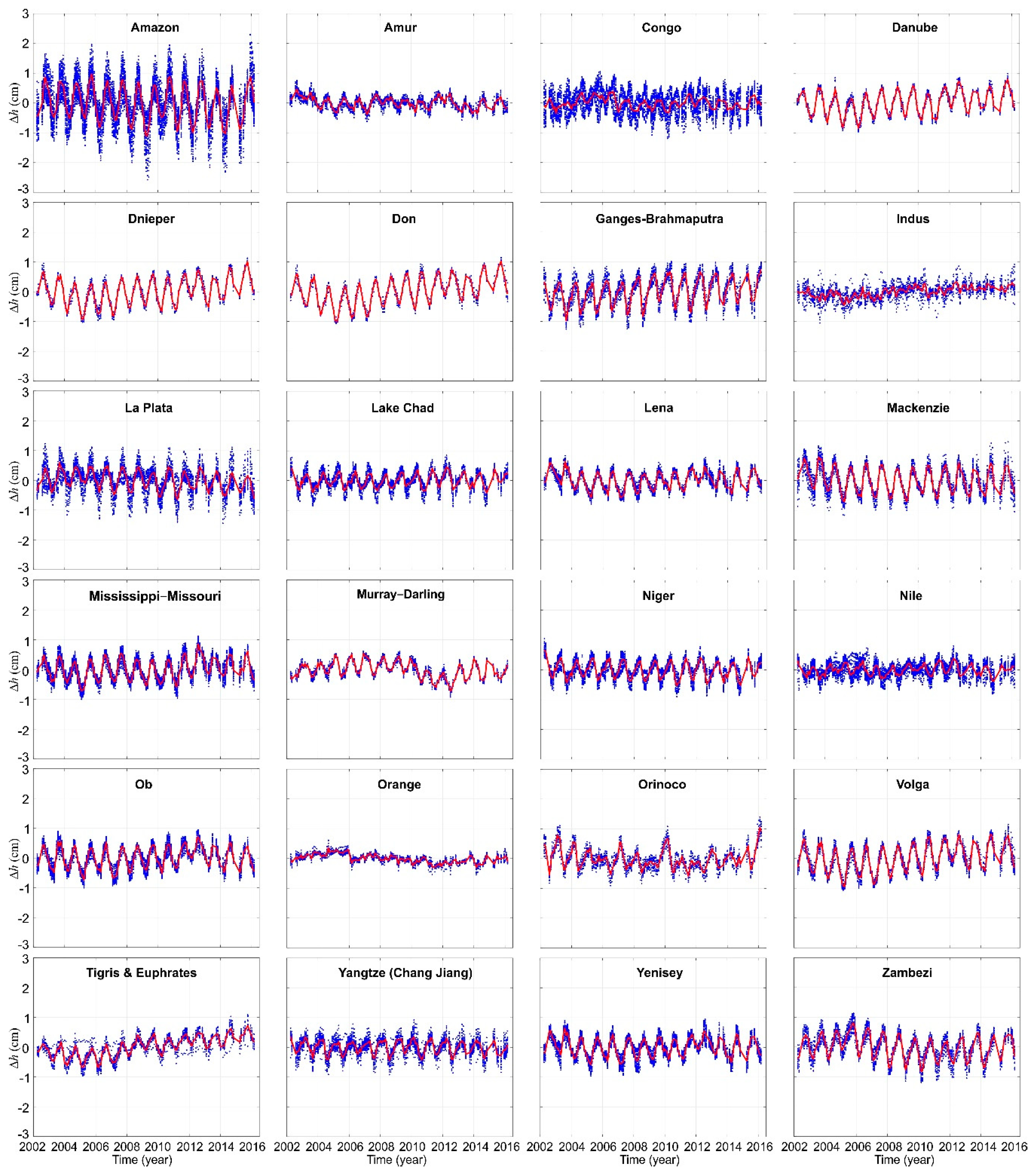
3.1. Orthometric/Normal Height Changes in the Time Domain

On the basis of GRACE satellite mission data, temporal variations of geoid/quasigeoid heights (Figure 3) and vertical deformations of the Earth’s surface (Figure 4) were estimated over large river basins specified in Figure 2 using Equations (4) and (5), respectively. These height changes were estimated with a high accuracy, as GRACE satellite mission data are sufficient to determine geoid height changes for a short period (i.e., less than 3 months) with an accuracy of 0.25 mm (see [68]). The phase shift between mean temporal variations of geoid/quasigeoid heights and mean vertical deformations of the Earth’s surface over large river basins investigated are depicted in Figure 5. The results presented in Figure 3 indicate that the amplitude of temporal variations of geoid/quasigeoid heights reach 8 mm over the Amazon basin, which agrees with the results presented in [26], and 2 mm over the Orange basin. The results presented in Figure 4 reveal that the amplitude of vertical deformations of the Earth’s surface reach the level of 13 mm over the Amazon basin, which agrees with the results given in [13], and 3 mm over the Orange basin. The amplitudes of temporal variations of geoid/quasigeoid heights and vertical deformations of the Earth’s surface for the remaining large river basins investigated are at the level of 5 mm, and 8 mm, respectively. Moreover, the results presented in Figure 3 and Figure 4 reveal that, for most of river basins investigated, seasonal patterns of temporal variations of geoid/quasigeoid heights are shifted in phase with respect to vertical deformations of the Earth’s surface by approximately 6 months (cf. Figure 5). This illustrates the relation between temporal variations of hydrological masses, temporal variations of geoid/quasigeoid heights and the crustal deformations in the vertical component. The ∆HH* over large river basins investigated (Figure 6) were determined by combining temporal variations of geoid/quasigeoid heights (cf. Figure 3) and vertical deformations of the Earth’s surface (cf. Figure 4). The dispersions (Max-Min) of ∆h, ∆N/∆ζ and ∆H/∆H* for the river basins investigated, taking into consideration all subareas within the river basin, are illustrated in Figure 7. The extreme values of ∆h, ∆N/∆ζ and ∆H/∆H* are almost symmetric in relation to their mean values that are approximately equal to zero. Figure 6 and Figure 7 show that pick-to-pick variations of ∆HH* differ significantly (e.g., ca. 8 cm for the Amazon basin and ca. 2 cm for the Orange basin) for large river basins investigated within this study. This is due to the significant difference between temporal variations of hydrological masses for these large river basins. At different epochs, the amplitudes of ∆HH* can reach up to ca. 40 mm, and at most 5 mm over the Amazon, and Orange river basins, respectively. For the remaining large river basins, these amplitudes do not exceed 13 mm. The results presented in Figure 6 also reveal that for the period between 2005 and 2016, secular patterns of ∆HH* appear over some large river basins, e.g., Danube, Dnieper, Don and Tigris and Euphrates river basins. These secular patterns are estimated to 1.5 ± 0.5 mm/year, and they are ascribed to the drought pattern over these river basins. Furthermore, Figure 6 exhibits, for some river basins, a good agreement between the average of ∆HH* over the whole area of the river basin and ∆HH* from individual subareas (i.e., individual cell of the JPL 3° equal-area mascon grid) of the river basin. For example, for the Danube, Dnieper, Don, Volga and Murray Darling river basins, differences between ∆H/∆H* at subareas of these basins with respect to their average of ∆HH* values are at the level of ±3 mm. For the remaining river basins, these differences become larger reaching almost ±10 mm for the Nile river basin, ±15 mm for the Congo and La Plata river basins, and ±20 mm for the Amazon river basin. This indicates that ∆H/∆H* over the entire river basins investigated (except for Danube, Dnieper, Don, Volga and Murray Darling river basins) significantly differ from one subarea to another. Additionally, for each subarea of large river basins investigated root mean squares (RMS) of Δh time series, RMS of ΔNζ time series and RMS of ΔHH* time series were estimated. The maximum and minimum of the RMS obtained for each large river basin investigated are provided in Table 1. For Danube, Dnieper, Don, Volga and Murray Darling river basins the range of RMS does not exceed 0.7 mm for ∆N/∆ζ, 1.0 mm for ∆h and 1.6 mm for ∆HH*. For the remaining river basins, the differences in RMS between subareas are from 1.0 mm for ∆N/∆ζ, 1.1 mm for ∆h and 2.3 mm for ∆HH*for Orange river basins to 6.5 mm for ∆N/∆ζ, 10.7 mm for ∆h and 17.3 mm for ∆HH*for the Amazon. This reveals that amplitudes of ∆h, ∆N/∆ζ and ∆H/∆H* at subareas over entire each of large river basins investigated (except the Danube, Dnieper, Don, Volga and Murray Darling river basins) are inconsistent.
In order to investigate the impact of temporal variations of water mass, represented by ∆EWT, on ∆H/∆H*, coefficients of correlations between ∆HH* and ∆EWT were computed. The WGHM was used as an independent source of data to estimate ∆EWT that are linearly related to the surface density coefficients used in Equation (5) (cf. [69]). In order to avoid the discrepancies in linear trends of mass changes estimated from WGHM and GRACE data, ∆EWT and ∆HH* were detrended. Figure 8 shows coefficients of correlations between detrended ∆HH* and detrended ∆EWT. It illustrates that at 48% of subareas (i.e., mascon locations) investigated, strong negative correlations between ∆HH* and ∆EWT (correlation coefficients ranging from −0.97 to −0.70) were obtained. Weak/moderate negative correlations between ∆HH* and ∆EWT (coefficients of correlation ranging from −0.69 to −0.30) were observed at 40% of subareas investigated. At ca. 9% of subareas investigated the coefficients of correlation obtained range from −0.29 to zero, while at 3% of subareas investigated positive values of correlation coefficients (from zero to +0.37) are observed. The subareas exhibiting no correlations between ∆HH* and ∆EWT (ca. 12% of subareas investigated) are mainly clustered in areas of week hydrological signals such as in southern Sahara. For a few subareas in Lena, Mackenzie, Ganges–Brahmaputra and Yangtze (Chang Jiang) river basins the reason of the observed lack of correlation between ∆HH* from GRACE satellite mission data and ∆EWT from the WGHM is not evident.

3.2. Orthometric/Normal Height Changes in the Space-Time Domain

As examples, spatio-temporal variations of orthometric/normal heights for large river basins of the strongest and weakest ∆EWT signal, i.e., for Amazon and Orange basins, normalized with their standard deviations were investigated. These spatio-temporal variations were obtained using the PCA method. In order to avoid gaps in ΔHH* time series, GRACE data from the period between January 2004 and December 2010 were used in the investigation. Figure 9 and Figure 10 show the results of the analysis of temporal variations of orthometric/normal heights ∆H/∆H* using the PCA method, i.e., the percentage of a total variance of ΔHH* and the first, second, third and fourth PC time series, for the Amazon, and Orange basins, respectively.
The results presented in Figure 9 reveal that, in terms of the percentage of a total variance of temporal variations of orthometric/normal heights reflected by PCA/EOFs, the first two PCs time series reflect ca. 97% of ΔHH* signal for the Amazon basin. The PC time series 1 accounts the largest variance, i.e., 77%, of the total signal. This is due to the fact that it recovers the dominant spatio–temporal component of the signal. It clearly illustrates seasonal variations of ∆HH* with minimum values in March–May and maximum values in September–November. This is because over the Amazon basin, the minimum and maximum values of ∆EWT were observed in March-May and September–November, respectively (e.g., [70,71,72]). It also shows that the largest ∆HH* can be seen in 2005 resulting from the extreme drought in 2005 [73], followed by minimum ∆HH* values due to the larger than usual flood that occurred in 2006 and 2009 [74]. Temporal variations of the PC time series 2 precede those of PC time series 1 in phase by about two months. According to [70,71,72], this phase delay is due to the fact that for the Amazon basin, the average rainfall maximum is in February while the maximum of water storage is delayed by ca. 2 months, peaking in March/April. The EOF1 reveals that the maximum EOF loading pattern is within the downstream area of the Amazon basin, i.e., the eastern and south–eastern parts of the Amazon basin that combines the effect of rainfall-induced soil moisture and groundwater variations and seasonally varying storage in surface water for the river and inundation areas [61]. In terms of the EOF2 the Amazon basin is divided into two distinguished parts, northern and southern one. The positive values of the EOF2 loading pattern are obtained for the northern part, while negative values of the EOF2 loading pattern for the southern part. This north–south division can be ascribed to the fact that the rainfall seasonality induced by the seasonal north–south migration of the Intertropical Convergence Zone (ITC), and the fact that the minimum water storage in the northern part of the Amazon basin in observed from December to February while in the southern part—from July to September. Overall, the first and second EOFs obtained illustrate clear differences between EOFs loading patterns for subareas of the entire Amazon basin.
The Orange basin, in contrary to the Amazon basin, is characterized by the weakest signal of ΔHH* among the river basins investigated (cf. Figure 7). This is because ΔEWT obtained from GRACE satellite mission data over this basin are very weak [75]. This might be ascribed to the fact that the majority of the Orange basin is covered by desert areas, i.e., Kalahari Desert and Namib Desert. The weakest ΔHH* signals over the Orange basin are observed. The results presented in Figure 10 indicate that in terms of the percentage of a total variance of ∆H/∆H* reflected by PCAs, the PC time series 1 reflects ca. 85% of ΔHH* signal and the second one reflects ca. 9% of ΔHH* signal for the Orange basin. They recover the dominant spatio-temporal component of the ΔHH* signal over the Orange basin. For the PC time series 1, a downward trend is observed and also a sharp fall at the end of 2005 and the beginning of 2006 is clearly noticeable. At that time there were heavy rains that caused flooding in the area of Southern Africa [76]. In the case of the PC time series 2, for the period 2005–2011, a distinct seasonal pattern is observed. This seasonal pattern coincides with the wet, and dry seasons, respectively, over the Orange basin, and it might be attributed to the seasonal runoff linked with climatic conditions within the Orange basin [77]. For 2004, this seasonal pattern is unclear. This might be ascribed to the fact that practically no rainfall was recorded in the fall season of 2004 over Orange basin [76]. The EOF1 reveals that the maximum EOF loading values occur in the north-eastern part of the Orange basin, whereas the minimum values were obtained for the south–western part. There is a slope from north-eastern to south-western in the EOF1 pattern. It means that subareas, located in the north-eastern part of the basin, have the major impact on PC time series 1. This is because in the north-eastern part of the Orange basin, the annual rainfall exceeds the annual evaporation, and thereby, induces significant run off [77]. On the contrary, in the south-western part of the Orange basin the annual evaporation exceeds the annual rainfall [77]. Moreover, the northern catchment areas of the Orange basin are characterized with a relatively high rainfall, while the central and southern catchments areas of the basin are characterized with lower rainfall and high evaporation. Therefore, relatively strong water mass variations signal induced from the northern catchment areas are not explained by PC time series 1 in the central and southern catchment areas of the basin [78]. The opposite situation takes place in the case of the EOF2. The descending slope of loading pattern from south-western to north-eastern is observed, and thus subareas located in the south–west have the biggest impact on PC time series 2. This is due to the fact that the topography and climate of the Orange basin varies significantly, i.e., from mountains to flat areas and from moist sub-humid to hyper-arid (deserts) climate zones, from northern to southern catchment areas [67]. Furthermore, 75% of the annual runoff occurs during summer months and 25% of the runoff occurs during winter [77]. The lower part of the Orange basin is also characterized by a complex geological structure [77], and therefore, the EOF2 pattern may be attributed to the geological structure and climatic conditions prevailing in southern Orange basin.
It should be noted that over the Amazon basin, the third and fourth PCs time series accounts for 3%, and 1% of total variance of ΔHH* signal, respectively. For the Orange basin, total variances of ΔHH* signal were at the level of 3% for the third PC time series and the level of 2% for the fourth PC time series. In terms of total variance of ΔHH* signal, the third and fourth PCA/EOFs can be considered insignificant in comparison to the first and second PCs time series. Furthermore, the summation of total variances of ΔHH* signal for the remaining 5th to 75th PCs time series for the Amazon basin and the summation of total variances of ΔHH* signal for the remaining 5th to 15th PCs time series over the Orange basin are at the level of 1%. Therefore, the analysis of these remaining PCs time series were neglected in this investigation.

4. Discussion and Conclusions
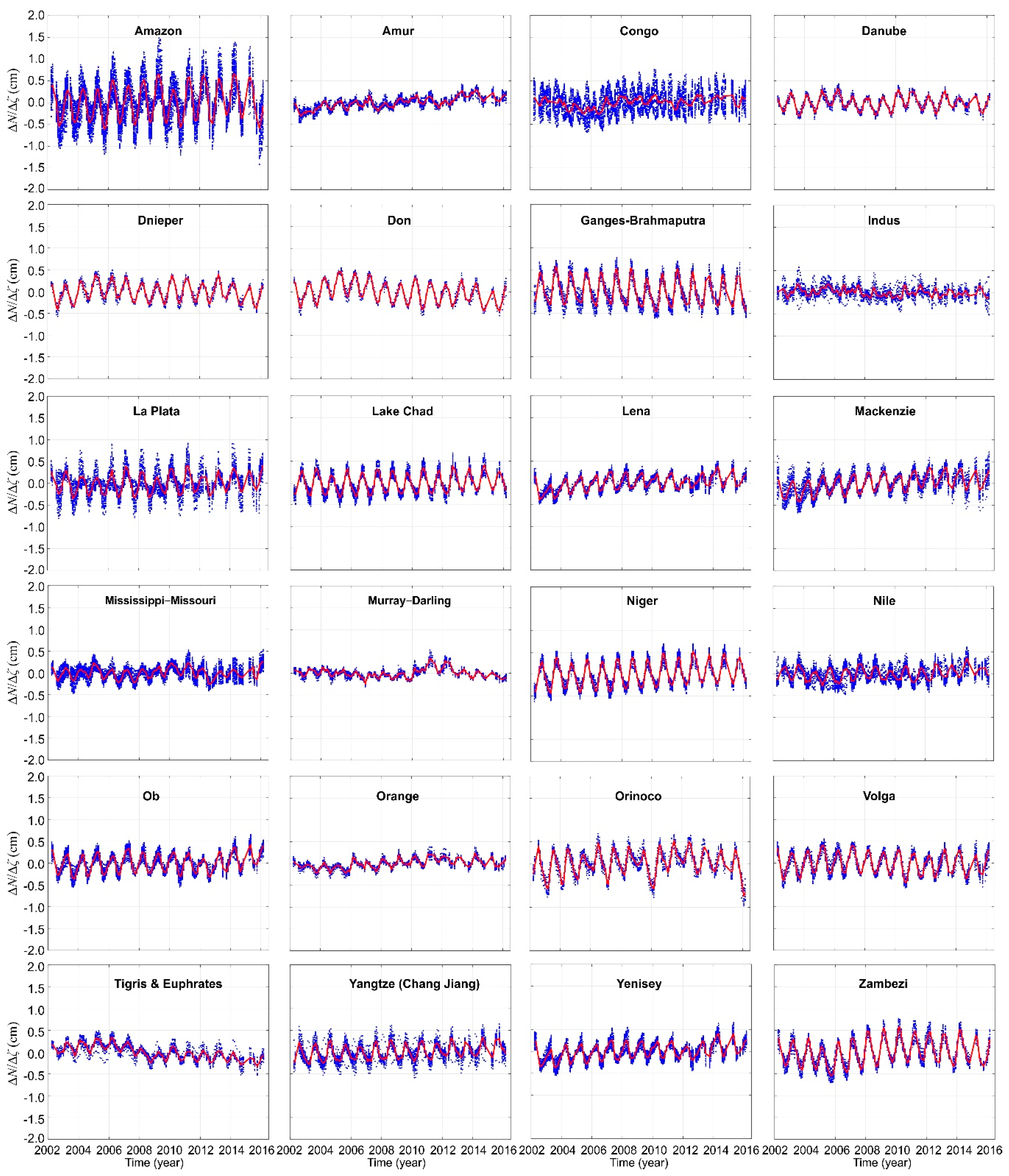
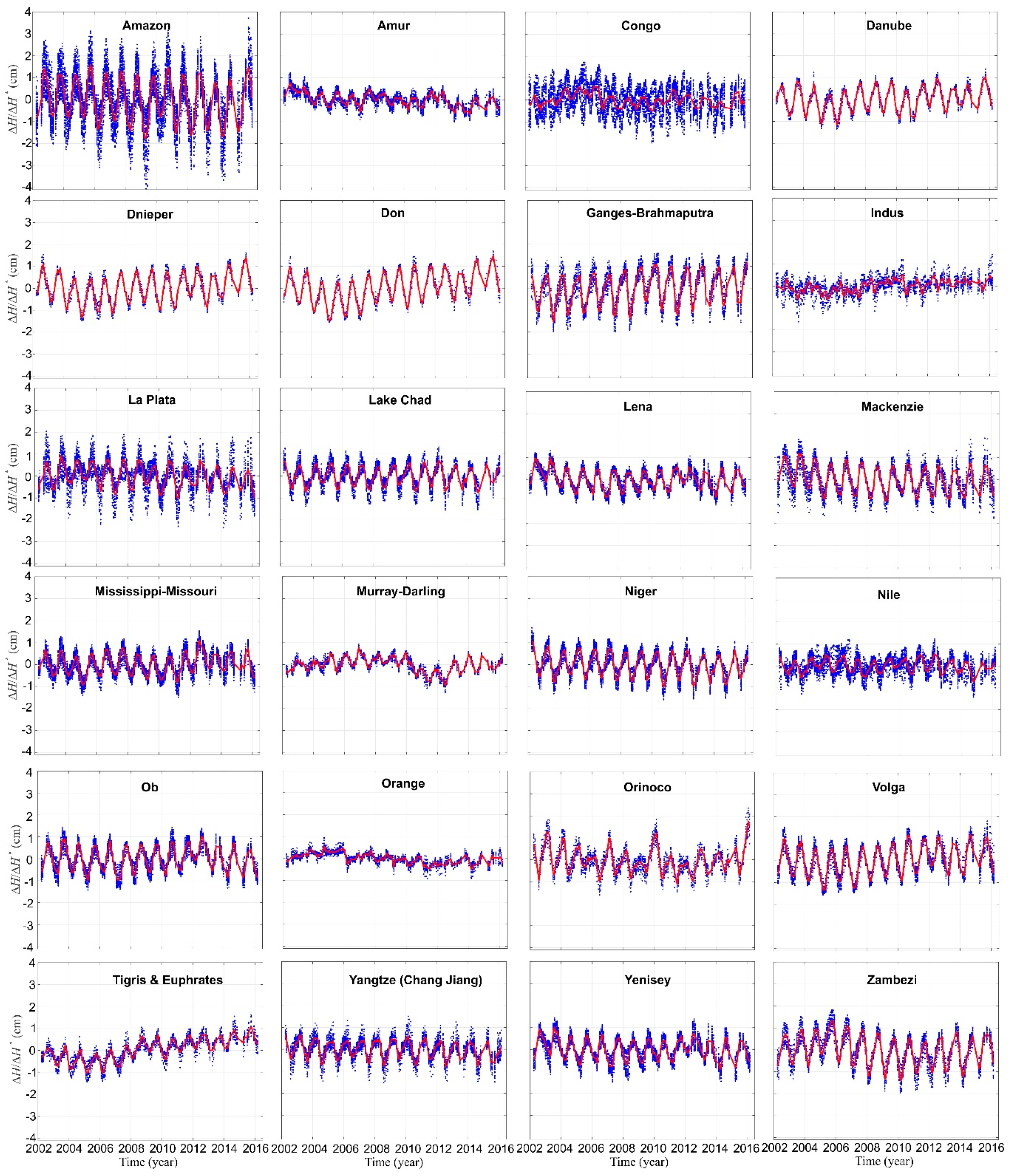
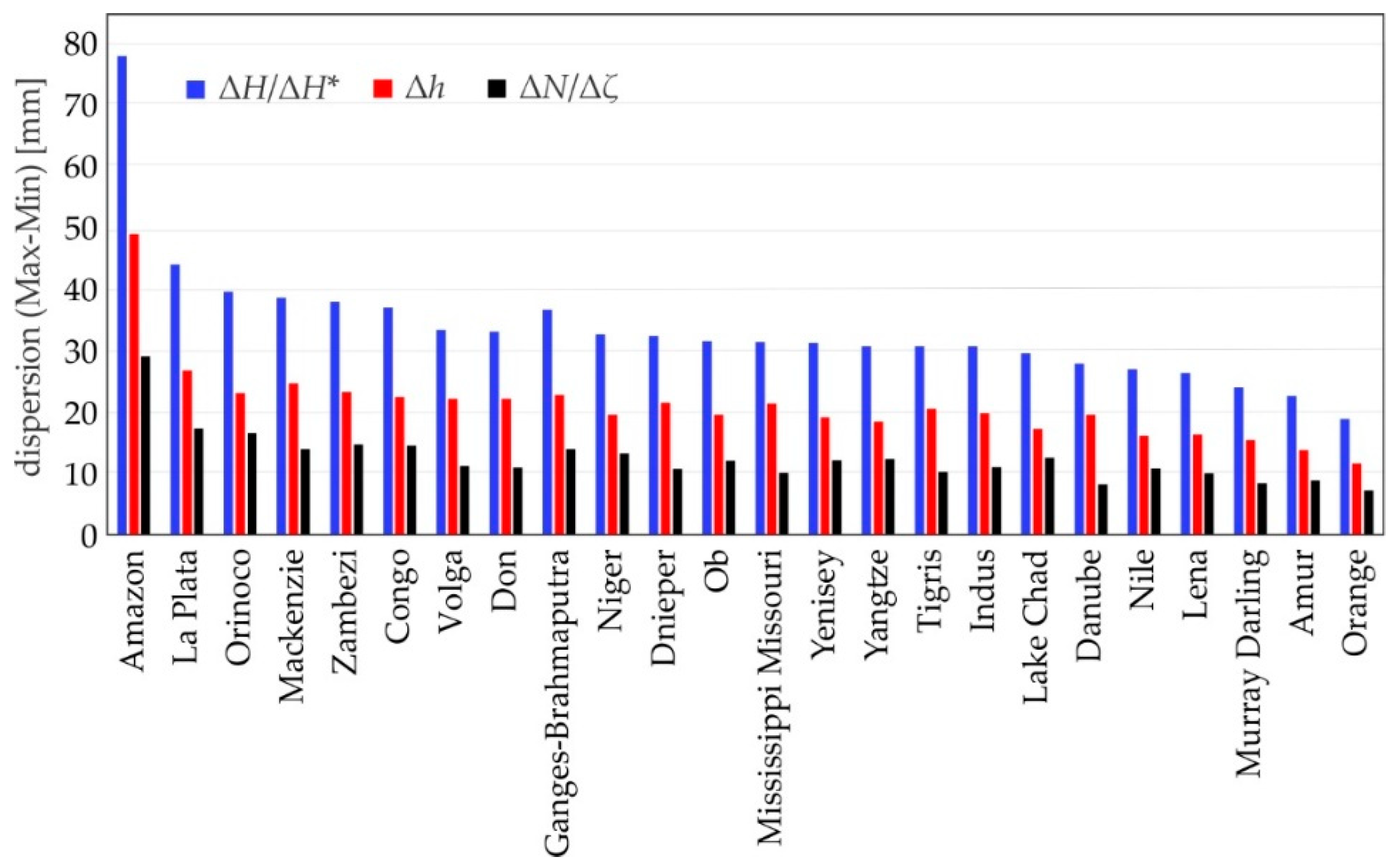
Although, orthometric/normal heights are considered static over the majority of the Earth land areas, except in areas of land uplift, temporal mass variations within the Earth’s system result in both temporal variations of geoid/quasigeoid heights and vertical deformations of the Earth’s surface, and thereby, temporal variations of orthometric/normal heights. Considering the fact that approximately half of the Earth’s land areas are covered by large river basins, in this study, temporal variations of orthometric/normal heights ΔHH* for 24 large river basins over the world were determined using GRACE-based GGMs. These ΔHH* are needed to correct orthometric/normal heights. Correlations between these ΔHH* and temporal variations of equivalent water thickness ∆EWT obtained from the WGHM hydrological model were investigated. The spatio-temporal analysis of ΔHH* for two river basinsn characterized by the strongest and the weakest ΔHH* signaln was conducted using the PC method.
The main findings of the research are as follows:
  • Amplitudes of ΔHH* significantly differ from each other between large river basins investigated. The largest amplitudes were obtained for river basins located over tropical rainforests, whilst the lowest ones were observed over desert areas. This is due to the fact that hydrological mass changes within large river basins located in the tropical rain forest are substantially larger than the ones over desert areas. For example, the range of ΔHH* for the same subarea at different epochs reaches 8 cm over the Amazon basin and only ca. 2 cm for the Orange basin.
  • For some large river basins ΔHH* time series obtained for particular subareas of the river basin are similar and close to each other, e.g., Danube, Dnieper and Don basins. This is because the hydrological mass changes patterns over the entire large river basins are consistent. However, in many cases differences between ΔHH* obtained at subareas within the same river basin are significant, sometimes exceeding three times the amplitude of the average of ΔHH* over the whole river basin, e.g., for the Congo basin. This is due to the fact that hydrological mass changes patterns substantially differ among subareas located in the same large river basin.
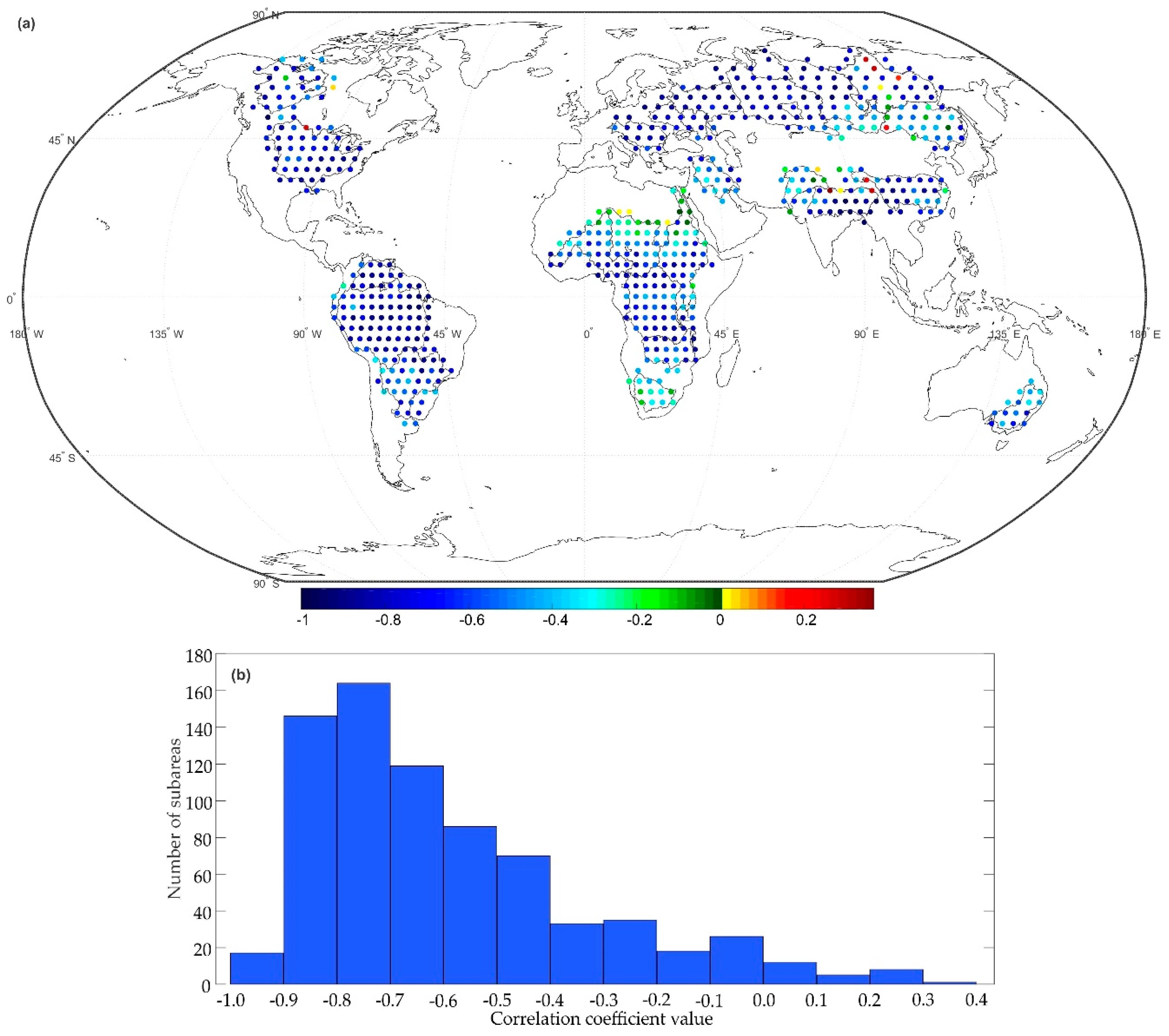
  • For 88% of river basins subareas negative correlations between detrended ΔHH* and detrended ∆EWT were observed, whereas they are strong for 48% of those subareas. This is because the increase of hydrological masses results in decrease of ΔHH*, and vice versa, the decrease of hydrological masses results in increase of ΔHH*. For the remaining 12% of river basins subareas there are no correlations between detrended ∆HH* and detrended ∆EWT. The main reason for observing no correlations can be ascribed to the fact that the majority of those subareas are located in regions of a very weak hydrological signal (e.g., southern Sahara). However, further investigations concerning the correlation between ∆HH* from GRACE satellite mission data and ∆EWT from the WGHM for some subareas such as the ones located in Lena, Mackenzie and Ganges–Brahmaputra river basins are recommended.
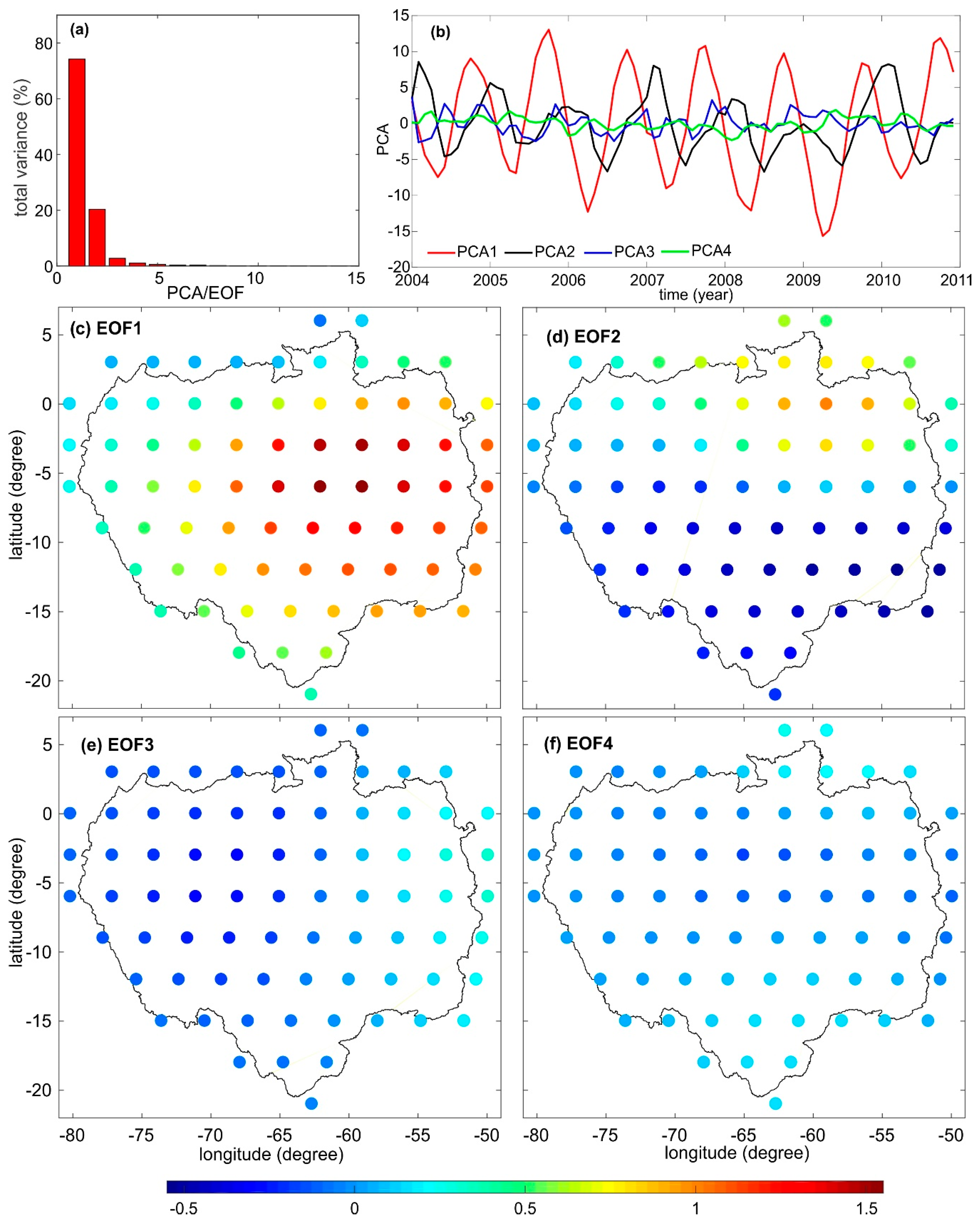
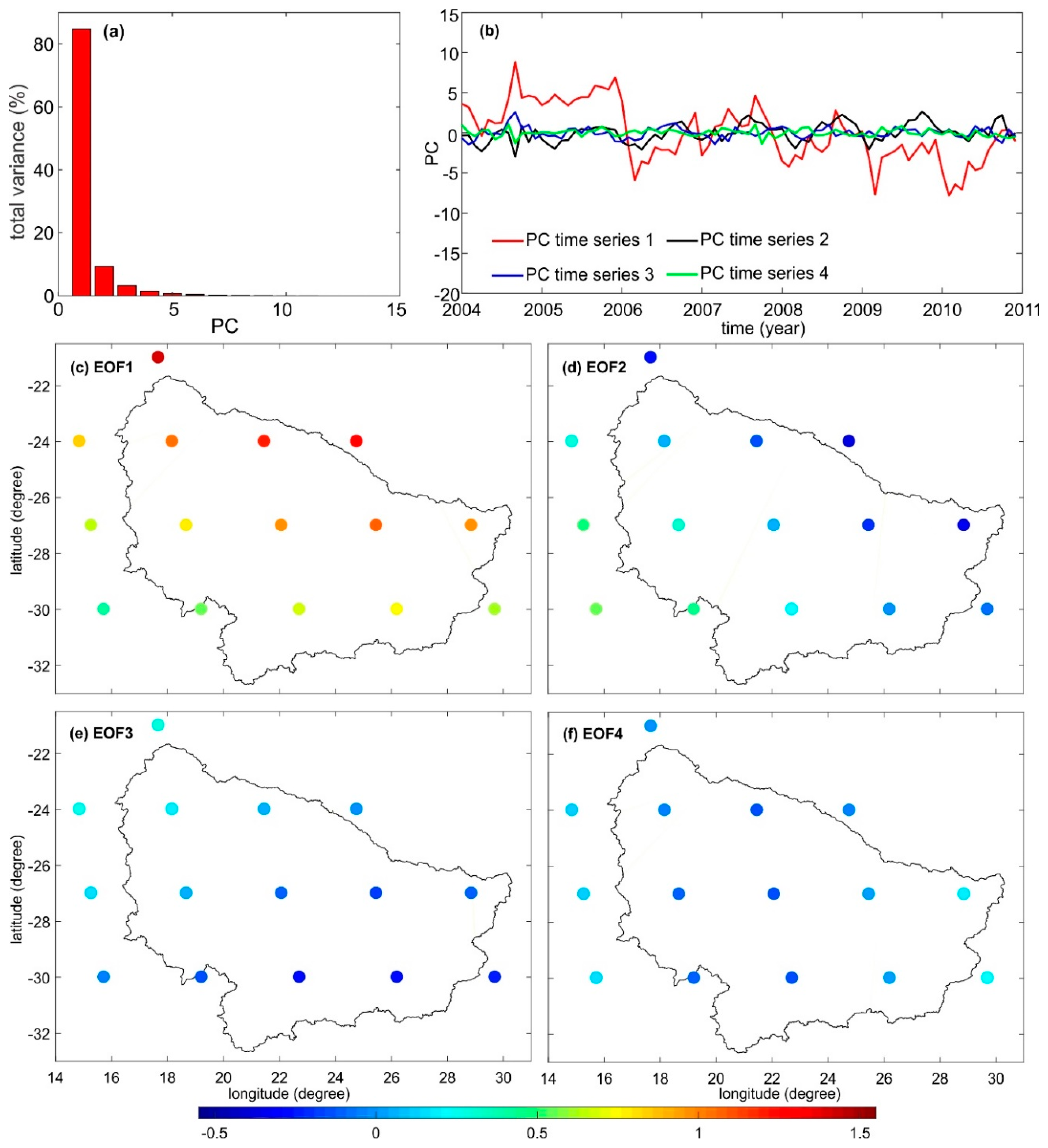
  • For Amazon and Orange basins, the 1st and 2nd PCs time series reflect together 95%, and 94% of a total variance of ΔHH* signal, respectively. Although, these percentages are close to each other, the contribution of the first and second PCs time series is different in the case of both river basins, i.e., the first and second PCs time series are 77%, and 20%, respectively, for the Amazon basin, and the first and second PCs time series are 85% and 9%, respectively, for the Orange basin. The first and second PCs time series exhibit that ∆H/∆H* are not an artefact, but are a consequence of the processes inducing hydrological mass transport. These temporal variations of orthometric/normal heights are strongly associated to different spatio–temporal patterns of the entire river basins. They can be associated with the extreme drought, the unusual flood, the location of the upstream and downstream areas of the river basin, the rainfall seasonality induced by the seasonal migration of the Intertropical Convergence Zone (ITC) and other climatic conditions, the spatial distribution of the water storage of the entire river basin and the geological structure of the river basin.
Overall, the results obtained in this investigation clearly prove that GRACE satellite mission data are significant for determining ∆H/∆H* induced by temporal variations of hydrological masses over large river basins. These temporal variations are needed for precise determination of orthometric/normal heights to monitor, interpret, analyse and model changes in those heights used in scientific (e.g., crustal motion, subsidence and isostatic readjustment) and engineering (e.g., the deformation of bridges, dams and large constructions) works, especially for areas characterized with significant temporal mass variations within the Earth’s system such as hydrological masses in large basins.

Author Contributions

Conceptualization, W.G., M.S. and J.K.; data acquisition, W.G., M.S. and J.D.R.; methodology, W.G., M.S. and J.K.; software, W.G.; results analysis, W.G., M.S. and J.D.R.; visualization, W.G.; writing, reviewing and editing, W.G., M.S., J.D.R. and J.K.; funding Acquisition, W.G., M.S. and J.K. All authors have read and agree to the published version of the manuscript.

Funding

This work was supported by the Polish National Science Centre (NCN) within the research Grant No. 2017/26/D/ST10/00422.

Acknowledgments

The authors would like to acknowledge the anonymous three reviewers for their valuable and constructive comments.

Conflicts of Interest

The authors declare no conflict of interest.

References

  1. Farahani, H.H.; Klees, R.; Slobbe, C. Data requirements for a 5–mm quasi–geoid in The Netherlands. Stud. Geophys. Geod. 2017, 61, 675–702. [Google Scholar] [CrossRef]
  2. Foroughi, I.; Vaníček, P.; Kingdon, R.W.; Goli, M.; Sheng, M.; Afrasteh, Y.; Novák, P.; Santos, M.C. Sub-centimetre geoid. J. Geod. 2019, 93, 849–868. [Google Scholar] [CrossRef]
  3. Ellmann, A.; Märdla, S.; Oja, T. The 5 mm geoid model for Estonia computed by the least squares modified Stokes’s formula. Surv. Rev. 2019, 52, 352–372. [Google Scholar] [CrossRef]
  4. Drewes, H.; Kuglitsch, F.; Adám, J.; Rózsa, S. The Geodesist’s handbook 2016. J. Geod. 2016, 90, 907–1205. [Google Scholar] [CrossRef]
  5. Li, X.; Zhang, X.; Ren, X.; Fritsche, M.; Wickert, J.; Schuh, H. Precise positioning with current multi-constellation Global Navigation Satellite Systems: GPS, GLONASS, Galileo and BeiDou. Sci. Rep. 2015, 5, 8328. [Google Scholar] [CrossRef] [PubMed]
  6. Heiskanen, W.; Moritz, H. Physical Geodesy; WH Freeman: San Francisco, CA, USA, 1967. [Google Scholar]
  7. Godah, W.; Szelachowska, M.; Krynski, J. Investigation of geoid height variations and vertical displacements of the Earth surface in the context of the realization of the modern vertical reference system —A case study for Poland. Int. Assoc. Geod. Symp. 2019, 148, 135–141. [Google Scholar] [CrossRef]
  8. Godah, W.; Szelachowska, M.; Krynski, J. Application of the PCA/EOF method for the analysis and modelling of temporal variations of geoid heights over Poland. Acta Geod. Geophys. 2018, 53, 93–105. [Google Scholar] [CrossRef]
  9. Godah, W. IGiK–TVGMF: A MATLAB package for computing and analysing temporal variations of gravity/mass functionals from GRACE satellite based global geopotential models. Comput. Geosci. 2019, 123, 47–58. [Google Scholar] [CrossRef]
  10. Zeray Öztürk, E.; Godah, W.; Abbak, R.A. Estimation of Physical Height Changes from GRACE Satellite Mission Data and WGHM over Turkey. Acta Geod. Geophys. 2020, 55, 301–317. [Google Scholar] [CrossRef]
  11. Tapley, B.D.; Bettadpur, S.; Watkins, M.; Reigber, C. The gravity recovery and climate experiment: Mission overview and early results. Geophys. Res. Lett. 2004, 31, L09607. [Google Scholar] [CrossRef] [Green Version]
  12. Kornfeld, R.P.; Arnold, B.W.; Gross, M.A.; Dahya, N.T.; Klipstein, W.M.; Gath, P.F.; Bettadpur, S. GRACE-FO: The Gravity Recovery and Climate Experiment Follow-On Mission. J. Spacecr. Rocket. 2019, 56, 931–951. [Google Scholar] [CrossRef]
  13. Tapley, B.D.; Bettadpur, S.; Ries, S.C.; Thompson, P.F.; Watkins, M.M. GRACE Measurements of Mass Variability in the Earth System. Science 2004, 305, 503–505. [Google Scholar] [CrossRef] [PubMed] [Green Version]
  14. Rangelova, E. A Dynamic Geoid Model for Canada. PhD. Thesis, Department of Geomatics Engineering, University of Calgary, Calgary, AB, Canada, 2007. [Google Scholar]
  15. Rangelova, E.; Fotopoulos, G.; Sideris, M.G. Implementing a dynamic geoid as a vertical datum for orthometric heights in Canada. Int. Assoc. Geod. Symp. 2010, 135, 295–302. [Google Scholar] [CrossRef]
  16. Rangelova, E.; Sideris, M.G. Contributions of terrestrial and GRACE data to the study of the secular geoid changes in North America. J. Geodyn. 2008, 46, 131–143. [Google Scholar] [CrossRef]
  17. Krynski, J.; Kloch-Główka, G.; Szelachowska, M. Analysis of time variations of the gravity field over Europe obtained from GRACE data in terms of geoid height and mass variations. Int. Assoc. Geod. Symp. 2014, 139, 365–370. [Google Scholar] [CrossRef]
  18. Godah, W.; Szelachowska, M.; Krynski, J. On the estimation of physical height changes using GRACE satellite mission data—A case study of Central Europe. Geod. Cartogr. 2017, 66, 211–226. [Google Scholar] [CrossRef] [Green Version]
  19. Godah, W.; Szelachowska, M.; Krynski, J. On the analysis of temporal geoid height variations obtained from GRACE–based GGMs over the area of Poland. Acta Geophys. 2017, 65, 713–725. [Google Scholar] [CrossRef] [Green Version]
  20. Kusche, J.; Schrama, E. Surface mass redistribution inversion from global GPS deformation and Gravity Recovery and Climate Experiment (GRACE) gravity data. J. Geophys. Res. 2005, 110, B09409. [Google Scholar] [CrossRef] [Green Version]
  21. Tregoning, P.; Watson, C.; Ramillien, G.; McQueen, H.; Zhang, J. Detecting hydrologic deformation using GRACE and GPS. Geophys. Res. Lett. 2009, 36, L15401. [Google Scholar] [CrossRef] [Green Version]
  22. Rietbroek, R.; Fritsche, M.; Dahle, C.; Brunnabend, S.E.; Behnisch, M.; Kusche, J.; Flechtner, F.; Schröter, J.; Dietrich, R. Can GPS-Derived Surface Loading Bridge a GRACE Mission Gap? Surv. Geophys. 2014, 35, 1267–1283. [Google Scholar] [CrossRef] [Green Version]
  23. van Dam, T.; Wahr, J.; Lavallée, D. A comparison of annual vertical crustal displacements from GPS and Gravity Recovery and Climate Experiment (GRACE) over Europe. J. Geophys. Res. 2007, 112, B03404. [Google Scholar] [CrossRef] [Green Version]
  24. Davis, J.L.; Elósegui, P.; Mitrovica, J.X.; Tamisiea, M.E. Climate-driven deformation of the solid earth from GRACE and GPS. Geophys. Res. Lett. 2004, 31, L24605. [Google Scholar] [CrossRef] [Green Version]
  25. Bevis, M.; Alsdorf, D.; Kendrick, E.; Fortes, L.P.; Forsberg, B.; Smalley, R., Jr.; Becker, J. Seasonal fluctuations in the mass of the Amazon River system and Earth’s elastic response. Geophys. Res. Lett. 2005, 32, L16308. [Google Scholar] [CrossRef] [Green Version]
  26. Knowles, L.A.; Bennett, R.A.; Harig, C. Vertical Displacements of the Amazon Basin from GRACE and GPS. J. Geophys. Res. Solid Earth 2020, 125, e2019JB018105. [Google Scholar] [CrossRef]
  27. Nahmani, S.; Bock, O.; Bouin, M.-N.; Santamaría-Gómez, A.; Boy, J.P.; Collilieux, X.; Métivier, L.; Panet, I.; Genthon, P.; De Linage, C.; et al. Hydrological deformation induced by the West African Monsoon: Comparison of GPS, GRACE and loading models. J. Geophys. Res. Solid Earth 2012, 117, B05409. [Google Scholar] [CrossRef] [Green Version]
  28. Birhanu, Y.; Bendick, R. Monsoonal loading in Ethiopia and Eritrea from vertical GPS displacement time series. J. Geophys. Res. Solid Earth 2015, 120, 7231–7238. [Google Scholar] [CrossRef] [Green Version]
  29. Heki, K. Dense GPS array as a new sensor of seasonal changes of surface loads. Geophys. Monogr. Ser. 2004, 150, 177–196. [Google Scholar] [CrossRef] [Green Version]
  30. Steckler, M.S.; Nooner, S.L.; Akhter, S.H.; Chowdhury, S.K.; Bettadpur, S.; Seeber, L.; Kogan, M.G. Modeling Earth deformation from monsoonal flooding in Bangladesh using hydrographic, GPS, and Gravity Recovery and Climate Experiment (GRACE) data. J. Geophys. Res. Solid Earth 2010, 115, B08407. [Google Scholar] [CrossRef]
  31. Liu, R.L.; Li, J.; Fok, H.S.; Shum, C.K.; Li, Z. Earth surface deformation in the North China plain detected by joint analysis of GRACE and GPS data. Sensors 2014, 14, 19861–19876. [Google Scholar] [CrossRef] [Green Version]
  32. Zhang, B.; Yao, Y.; Fok, H.S.; Hu, Y.; Chen, Q. Potential seasonal terrestrial water storage monitoring from GPS vertical displacements: A case study in the lower three-rivers headwater region, China. Sensors 2016, 16, 1526. [Google Scholar] [CrossRef]
  33. Jiang, W.; Yuan, P.; Chen, H.; Cai, J.; Li, Z.; Chao, N.; Sneeuw, N. Annual variations of monsoon and drought detected by GPS: A case study in Yunnan, China. Sci. Rep. 2017, 7, 5874. [Google Scholar] [CrossRef] [PubMed]
  34. Zou, R.; Wang, Q.; Freymueller, J.T.; Poutanen, M.; Cao, X.; Zhang, C.; Yang, S.; He, P. Seasonal hydrological loading in southern Tibet detected by joint analysis of GPS and GRACE. Sensors 2015, 15, 30525–30538. [Google Scholar] [CrossRef] [PubMed]
  35. Pan, Y.; Shen, W.B.; Hwang, C.; Liao, C.; Zhang, T.; Zhang, G. Seasonal Mass Changes and Crustal Vertical Deformations Constrained by GPS and GRACE in Northeastern Tibet. Sensors 2016, 16, 1211. [Google Scholar] [CrossRef] [PubMed] [Green Version]
  36. Rajner, M.; Liwosz, T. Studies of crustal deformation due to hydrological loading on GPS height estimates. Geod. Cartogr. 2011, 60, 135–144. [Google Scholar] [CrossRef] [Green Version]
  37. Godah, W.; Szelachowska, M.; Ray, J.D.; Krynski, J. Comparison of vertical deformations of the Earth’s surface obtained using GRACE-based GGMs and GNSS data—A case study of Poland. Acta Geodyn. Geomater. 2020, 17, 169–176. [Google Scholar] [CrossRef]
  38. Bevis, M.; Wahr, J.; Khan, S.A.; Madsen, F.B.; Brown, A.; Willis, M.; Kendrick, E.; Knudsen, P.; Box, J.E.; van Dam, T.; et al. Bedrock displacements in Greenland manifest ice mass variations, climate cycles and climate change. Proc. Natl. Acad. Sci. USA 2012, 109, 11944–11948. [Google Scholar] [CrossRef] [Green Version]
  39. Fu, Y.; Freymueller, J.T.; Jensen, T. Seasonal hydrological loading in southern Alaska observed by GPS and GRACE. Geophys. Res. Lett. 2012, 39, L15310. [Google Scholar] [CrossRef] [Green Version]
  40. Chew, C.C.; Small, E.E. Terrestrial water storage response to the 2012 drought estimated from GPS vertical position anomalies. Geophys. Res. Lett. 2014, 41, 6145–6151. [Google Scholar] [CrossRef]
  41. Fu, Y.; Argus, D.F.; Landerer, F.W. GPS As an Independent Measurement to Estimate Terrestrial Water Storage Variations in Washington and Oregon. J. Geophys. Res. Solid Earth 2015, 120, 552–566. [Google Scholar] [CrossRef]
  42. Tan, W.; Dong, D.; Chen, J.; Wu, B. Analysis of systematic differences from GPS-measured and GRACE-modeled deformation in Central Valley, California. Adv. Space Res. 2016, 57, 19–29. [Google Scholar] [CrossRef]
  43. Eriksson, D.; MacMillan, D.S. Continental hydrology loading observed by VLBI measurements. J. Geod. 2014, 88, 675–690. [Google Scholar] [CrossRef]
  44. Öztürk, E.Z.; Abbak, R.A. PHCSOFT: A Software package for computing physical height changes from GRACE based global geopotential models. Earth Sci. Inform. 2020, 2, 1–7. [Google Scholar] [CrossRef]
  45. Fotopoulos, G. An Analysis on the Optimal Combination of Geoid, Orthometric and Ellipsoidal Height Data. PhD Thesis, Department of Geomatics Engineering, University of Calgary, Calgary, AB, Canada, 2003. [CrossRef]
  46. Fuhrmann, T.; Westerhaus, M.; Zippelt, K.; Heck, B. Vertical displacement rates in the Upper Rhine Graben area derived from precise leveling. J. Geod. 2014, 88, 773–787. [Google Scholar] [CrossRef]
  47. Mäkinen, J.; Saaranen, V. Determination of post-glacial land uplift from the three precise levellings in Finland. J. Geod. 1998, 72, 516–529. [Google Scholar] [CrossRef]
  48. Bettadpur, S. Gravity Recovery and Climate Experiment Level–2 Gravity Field Product User Handbook. Center for Space Research at The University of Texas at Austin. Available online: ftp://podaac-ftp.jpl.nasa.gov/allData/grace/docs/L2-UserHandbook_v4.0.pdf (accessed on 18 September 2020).
  49. Dziewonski, A.M.; Anderson, D.L. Preliminary reference Earth model. Phys. Earth Planet. Inter. 1981, 25, 297–356. [Google Scholar] [CrossRef]
  50. Sun, Y.; Riva, R.; Ditmar, P. Optimizing estimates of annual variations and trends in geocenter motion and J2 from a combination of GRACE data and geophysical models. J. Geophys. Res. Solid Earth 2016, 121, 8352–8370. [Google Scholar] [CrossRef] [Green Version]
  51. Cheng, M.K.; Tapley, B.D.; Ries, J.C. Deceleration in the Earth’s oblateness. J. Geophys. Res. Solid Earth 2013, 118, 740–747. [Google Scholar] [CrossRef]
  52. Kusche, J.; Schmidt, R.; Petrovic, S.; Rietbroek, R. Decorrelated GRACE time–variable gravity solutions by GFZ, and their validation using a hydrological model. J. Geod. 2009, 83, 903–913. [Google Scholar] [CrossRef] [Green Version]
  53. Göttl, F.; Schmidt, M.; Seitz, F. Mass-related excitation of polar motion: An assessment of the new RL06 GRACE gravity field models. Earth Planets Space 2018, 70, 195. [Google Scholar] [CrossRef]
  54. Kvas, A.; Behzadpour, S.; Ellmer, M.; Klinger, B.; Strasser, S.; Zehentner, N.; Mayer-Gürr, T. ITSG-Grace2018: Overview and Evaluation of a New GRACE-Only Gravity Field Time Series. J. Geophys. Res. Solid Earth 2019, 124, 9332–9344. [Google Scholar] [CrossRef] [Green Version]
  55. Adhikari, S.; Ivins, E.R.; Frederikse, T.; Landerer, F.W.; Caron, L. Sea-level fingerprints emergent from GRACE mission data. Earth Syst. Sci. Data 2019, 11, 629–646. [Google Scholar] [CrossRef] [Green Version]
  56. Barthelmes, F. Definition of Functionals of the Geopotential and their Calculation from Spherical Harmonic Models: Theory and Formulas Used by the Calculation Service of the International Centre for Global Earth Models (ICGEM); Scientific Technical Report STR09/02; GFZ German Research Centre for Geosciences: Potsdam, Germany, 2013; p. 32. Available online: http://icgem.gfz-potsdam.de (accessed on 18 September 2020).
  57. Zhang, X.; Jin, S.; Lu, X. Global Surface Mass Variations from Continuous GPS Observations and Satellite Altimetry Data. Remote Sens. 2017, 9, 1000. [Google Scholar] [CrossRef] [Green Version]
  58. Müller Schmied, H. Evaluation, modification and application of a global hydrological model. In Frankfurt Hydrology Paper 16; Institute of Physical Geography, Goethe University Frankfurt: Frankfurt am Main, Germany; Available online: https://www.uni-frankfurt.de/65883413/Mueller_Schmied_2017_evaluation_modification_and_application_of_a_global_hydrological_model.pdf (accessed on 18 September 2020).
  59. Müller Schmied, H.; Eisner, S.; Franz, D.; Wattenbach, M.; Portmann, F.T.; Flörke, M.; Döll, P. Sensitivity of simulated global-scale freshwater fluxes and storages to input data, hydrological model structure, human water use and calibration. Hydrol. Earth Syst. Sci. 2014, 18, 3511–3538. [Google Scholar] [CrossRef] [Green Version]
  60. Döll, P.; Hoffmann-Dobrev, H.; Portmann, F.T.; Siebert, S.; Eicker, A.; Rodell, M.; Strassberg, G.; Scanlon, B.R. Impact of water withdrawals from groundwater and surface water on continental water storage variations. J. Geodyn. 2012, 59, 143–156. [Google Scholar] [CrossRef]
  61. Schmidt, R.; Petrovic, S.; Güntner, A.; Barthelmes, F.; Wünsch, J.; Kusche, J. Periodic components of water storage changes from GRACE and global hydrology models. J. Geophys. Res. Solid Earth 2008, 113, B08419. [Google Scholar] [CrossRef] [Green Version]
  62. Landerer, F.W.; Dickey, J.O.; Güntner, A. Terrestrial water budget of the Eurasian pan-Arctic from GRACE satellite measurements during 2003–2009. J. Geophys. Res. Atmos. 2010, 115, D23115. [Google Scholar] [CrossRef] [Green Version]
  63. Döll, P.; Fritsche, M.; Eicker, A.; Müller Schmied, H. Seasonal water storage variations as impacted by water abstractions: Comparing the output of a global hydrological model with GRACE and GPS observations. Surv. Geophys. 2014, 35, 1311–1331. [Google Scholar] [CrossRef]
  64. Scanlon, B.R.; Zhang, Z.; Save, H.; Sun, A.Y.; Schmied, H.M.; Van Beek, L.P.; Wiese, D.N.; Wada, Y.; Long, D.; Reedy, R.C.; et al. Global models underestimate large decadal declining and rising water storage trends relative to GRACE satellite data. Proc. Natl. Acad. Sci. USA 2018, 115, E1080–E1089. [Google Scholar] [CrossRef] [Green Version]
  65. Jolliffe, I. Principal Component Analysis; Springer: New York, NY, USA, 2002. [Google Scholar]
  66. Li, J.; Wang, S.; Zhou, F. Time Series Analysis of Long-term Terrestrial Water Storage over Canada from GRACE Satellites Using Principal Component Analysis. Can. J. Remote Sens. 2016, 42, 161–170. [Google Scholar] [CrossRef]
  67. Preisendorfer, R.W.; Mobley, C.D. Principal Component Analysis in Meteorology and Oceanography; Elsevier: Amsterdam, The Netherlands, 1988. [Google Scholar]
  68. Schrama, E.J.O.; Visser, P.N.A.M. Accuracy assessment of the monthly GRACE geoids based upon a simulation. J. Geod. 2007, 81, 67–80. [Google Scholar] [CrossRef] [Green Version]
  69. Wahr, J.; Molenaar, M.; Bryan, F. Time variability of the Earth’s gravity field: Hydrological and oceanic effects and their possible detection using GRACE. J. Geophys. Res. 1998, 103, 30205–30229. [Google Scholar] [CrossRef]
  70. Zeng, N. Seasonal cycle and interannual variability in the Amazon hydrologic cycle. J. Geophys. Res. Atmos. 1999, 104, 9097–9106. [Google Scholar] [CrossRef]
  71. Chen, J.L.; Rodell, M.; Wilson, C.R.; Famiglietti, J.S. Low degree spherical harmonic influences on Gravity Recovery and Climate Experiment (GRACE) water storage estimates. Geophys. Res. Lett. 2005, 32, L14405. [Google Scholar] [CrossRef] [Green Version]
  72. Güntner, A.; Stuck, J.; Werth, S.; Döll, P.; Verzano, K.; Merz, B. A global analysis of temporal and spatial variations in continental water storage. Water Resour. Res. 2007, 43, W05416. [Google Scholar] [CrossRef]
  73. Tomasella, J.; Borma, L.S.; Marengo, J.A.; Rodriguez, D.A.; Cuartas, L.A.; ANobre, C.; Prado, M.C. The droughts of 1996–97 and 2004–5 in Amazonia: Hydrological response in the river main-stem. Hydrol. Process. 2011, 25, 1228–1242. [Google Scholar] [CrossRef]
  74. Chen, J.L.; Wilson, C.R.; Tapley, B.D. The 2009 exceptional Amazon flood and interannual terrestrial water storage change observed by GRACE. Water Resour. Res. 2010, 46, W12526. [Google Scholar] [CrossRef] [Green Version]
  75. Hasan, E.; Tarhule, A.; Zume, J.T.; Kirstetter, P.-E. +50 Years of Terrestrial Hydroclimatic Variability in Africa’s Transboundary Waters. Sci. Rep. 2019, 9, 12327. [Google Scholar] [CrossRef] [PubMed] [Green Version]
  76. SADC. Regional Flood Watch No. 1. January 2006. Available online: https://reliefweb.int/report/malawi/regional-flood-watch-no-1-jan-2006 (accessed on 31 July 2020).
  77. Diederichs, M.; Mander, M.; Caroline Sullivan, C.; dermot O’reagan, D.; mathew Fry, M.; Mckenzie, M. Orange River Basin—Baseline Vulnerability Assessment Report. NeWater. Available online: http://www.newater.uni-osnabrueck.de/intern/sendfile.php?id=1278 (accessed on 18 September 2020). [CrossRef]
  78. Hughes, D.A.A. Simple approach to estimating channel transmission losses in large South African river basin. J. Hydrol. Reg. Stud. 2019, 25, 100619. [Google Scholar] [CrossRef]
Figure 1. The relation between temporal variations of hydrological masses, temporal variations of geoid/quasigeoid heights and the crustal deformations in the vertical component, (a) Hydrological masses increase on the Earth’s surface, and (b) Hydrological masses decrease on the Earth’s surface.
Remotesensing 12 03070 g001
Figure 2. Map of large river basins investigated: (1) Amazon, (2) Amur, (3) Congo, (4) Danube, (5) Dnieper, (6) Don, (7) Ganges–Brahmaputra, (8) Indus, (9) La Plata, (10) Lake Chad, (11) Lena, (12) Mackenzie, (13) Mississippi–Missouri, (14) Murray–Darling, (15) Niger, (16) Nile, (17) Ob, (18) Orange, (19) Orinoco, (20) Volga, (21) Tigris & Euphrates, (22) Yangtze (Chang Jiang), (23) Yenisei and (24) Zambezi.
Remotesensing 12 03070 g002
Figure 3. Temporal variations for geoid/quasigeoid heights ∆N/∆ζ for twenty four large river basins investigated. Blue dots indicate ∆N/∆ζ values for subareas (i.e., JPL 3° equal-area mascon grid) within the river basin, whilst the red line indicates the mean ∆N/∆ζ over the whole river basin.
Remotesensing 12 03070 g003
Figure 4. Vertical deformations of the Earth’s surface ∆h for twenty four large river basins investigated. Blue dots indicate ∆h values for subareas (i.e., JPL 3° equal-area mascon grid) within the river basin, whilst the red line indicates the mean ∆h over the whole river basin.
Remotesensing 12 03070 g004
Figure 5. Phase shift between mean temporal variations of geoid/quasigeoid heights and mean vertical deformations of the Earth’s surface over large basins investigated.
Remotesensing 12 03070 g005
Figure 6. Temporal variations of orthometric/normal heights ∆HH* for twenty four large river basins investigated. Blue dots indicate ∆HH* values for subareas (i.e., mascon locations) within the river basin, whilst the red line indicates the average of ∆HH* over the whole river basin.
Remotesensing 12 03070 g006
Figure 7. The dispersion (Max-Min) of ∆h, ∆N/∆ζ and ∆H/∆H* over large river basins investigated [mm].
Remotesensing 12 03070 g007
Figure 8. Coefficients of correlations between ∆EWT obtained from the WGHM and ∆HH* determined using GRACE-based GGMs at subareas (i.e., JPL 3° equal-area mascon grid) of large river basins investigated, (a) Correlation coefficient values, and (b) Histogram of correlation coefficient values.
Remotesensing 12 03070 g008
Figure 9. PCA method results obtained using 75 time series of ∆H/∆H* normalized with their standard deviations over the Amazon basin: (a) Percentage of a total variance of ∆H/∆H* reflected by the first 15. PCs time series, (b) time series of the first, second, third and fourth PCs time series, (c) the first EOF loading pattern, (d) the second EOF loading pattern, (e) the third EOF loading pattern, and (f) the fourth EOF loading pattern.
Remotesensing 12 03070 g009
Figure 10. PCA method results obtained using 15 time series of ∆H/∆H* normalized with their standard deviations over the Orange basin: (a) percentages of a total variance of ∆H/∆H* reflected by the first 15 PCs time series, (b) time series of the first, second, third and fourth PCs time series, (c) the first EOF loading pattern, (d) the second EOF loading pattern, (e) the third EOF loading pattern, and (f) the fourth EOF loading pattern.
Remotesensing 12 03070 g010
Table 1. Maximum and minimum RMS of ∆h, ∆N/∆ζ and ∆H/∆H* time series for subareas of large river basins investigated [mm].
River BasinN/∆ζhH/∆H*
MaxMinMaxMinMaxMin
Amazon7.50.912.31.619.82.5
Amur1.80.92.91.34.52.0
Congo3.71.35.41.99.13.1
Danube1.91.34.23.66.04.8
Dnieper2.31.74.83.87.05.4
Don2.42.24.84.17.16.2
Ganges–Brahmaputra4.11.96.33.110.45.0
Indus2.20.83.91.46.02.0
Lake Chad3.31.14.21.47.32.1
La Plata4.91.17.31.812.22.1
Lena2.21.23.91.75.92.7
Mackenzie3.11.35.83.68.54.8
Mississippi–Missouri2.11.14.32.96.43.8
Murray Darling1.50.83.12.63.83.1
Niger3.31.24.11.57.32.3
Nile2.70.63.61.46.32.1
Ob2.60.74.71.47.01.8
Orange1.80.72.41.34.11.9
Orinoco3.61.74.72.18.23.7
Tigris2.41.14.61.66.93.3
Volga2.52.14.84.07.36.1
Yangtze3.61.05.21.48.72.4
Yenisey2.71.04.61.47.02.1
Zambezi3.71.95.62.29.24.0

