Temporal Gravity Signals in Reprocessed GOCE Gravitational Gradients


1
Chair of Astronomical and Physical Geodesy, Technical University of Munich, Arcisstraße 21, 80333 Munich, Germany
2
European Space Agency, Keplerlaan 1, 2201 AZ Noordwijk, The Netherlands
*
Author to whom correspondence should be addressed.
†
These authors contributed equally to this work.
Remote Sens. 2020, 12(21), 3483; https://0-doi-org.brum.beds.ac.uk/10.3390/rs12213483
Submission received: 3 September 2020
/
Revised: 10 October 2020
/
Accepted: 20 October 2020
/
Published: 23 October 2020
(This article belongs to the Special Issue Geodesy for Gravity and Height Systems)
Abstract
:The reprocessing of the satellite gravitational gradiometry (SGG) data from the Gravity field and steady-state Ocean Circulation Explorer (GOCE) satellite mission in 2018/2019 considerably reduced the low-frequency noise in the data, leading to reduced noise amplitudes in derived gravity field models at large spatial scales, at which temporal variations of the Earth’s gravity field have their highest amplitudes. This is the motivation to test the reprocessed GOCE SGG data for their ability to resolve time-variable gravity signals. For the gravity field processing, we apply and compare a spherical harmonics (SH) approach and a mass concentration (mascon) approach. Although their global signal-to-noise ratio is <1, SH GOCE SGG-only models resolve the strong regional signals of glacier melting in Greenland and Antarctica, and the 2011 moment magnitude 9.0 earthquake in Japan, providing an estimation of gravity variations independent of Gravity Recovery and Climate Experiment (GRACE) data. The benefit of combined GRACE/GOCE SGG models is evaluated based on the ice mass trend signals in Greenland and Antarctica. While no signal contribution from GOCE SGG data additional to the GRACE models could be observed, we show that the incorporation of GOCE SGG data numerically stabilizes the related normal equation systems.

1. Introduction
The satellite mission Gravity field and steady-state Ocean Circulation Explorer (GOCE [1]) collected data on the Earth’s gravity field from October 2009 to October 2013 [2], with the objective of determining the static global geoid on -level at a resolution of 100 half-wavelength ([1,3]). The main measurement principles of the GOCE mission are satellite gravitational gradiometry (SGG) and high-low satellite-to-satellite tracking (SST-hl). In this contribution, we exclusively focus on the SGG data, from which static gravity field models up to spherical harmonic (SH) degree and order (d/o) 280–300 can be derived [4].
The main purpose of the Gravity Recovery and Climate Experiment (GRACE) satellite mission, in contrast, was the determination of temporal variations of the Earth’s gravity field at a temporal resolution of one month and a spatial resolution of 400 to 40,000 km [5]. Due to its low-low satellite-to-satellite tracking (SST-ll) measurement system, GRACE data have an anisotropic sensitivity, leading to a characteristic longitudinal noise pattern in derived gravity field models [6].
The gravity field information derived from the GOCE and GRACE missions complement each other in the spatial domain, as shown by Figure 1: The intersection of the GRACE and GOCE degree error median curves at about SH degree shows that GRACE measurements are more sensitive to the large-scale gravity field while GOCE measurements are more sensitive to the medium-scale gravity field [7].
As temporal variations of the Earth’s gravity field predominantly take place on large spatial scales of several 100 , mainly GRACE models are used for studying the Earth’s gravity variations. However, because of their sensitivity to the shorter-wavelength gravity field, being able to use GOCE SGG data for time-variable signals would be beneficial in order to increase the spatial resolution of the signals as recovered from GRACE. Additionally, GOCE SGG data could complement GRACE data due to their isotropic sensitivity.
The goal to test GOCE SGG data for temporal gravity signals has been pursued for some time already (e.g., [11,12]). Moreover, the benefit of combining GRACE and GOCE data to increase the spatial resolution of time-variable signals resolved by GRACE was tested by previous studies ([12,13,14]). To our knowledge, all previous studies on the detectability of time-variable gravity signals in GOCE SGG data are based on the gradient data prior to the SGG data reprocessing in 2018/2019. Before this reprocessing campaign, the component of the SGG data suffered from a perturbing effect in the regions around the geomagnetic poles, which has been linked to thermospheric winds in these regions (see, e.g., in [15,16]). According to the authors of [17], this perturbation can be removed by introducing a quadratic function of the non-gravitational acceleration in y direction in the conversion from the control voltage measured by the electrostatic gradiometer to the derived acceleration. A detailed description of the improved SGG data calibration method that has been applied in the SGG data reprocessing in 2018/2019 is given by [18].
Figure 2 visualizes the improvements of the spectral properties of the measurement noise included in the component of the GOCE SGG data due to the reprocessing (we only present the noise spectra of the component here, as it shows the strongest improvements among the gradient components). Figure 2 shows that, on the one hand, the statistical properties of the SGG data become stationary over the complete mission period; on the other hand, the noise level in the low frequencies is considerably reduced, which can be expected to improve derived gravity field models at large spatial scales [4]. As time-variable gravity signals have their largest amplitudes in the long-wavelength range, due to the reprocessing, an improved ability of GOCE SGG data to resolve these signals can be anticipated. According to the work in [18], a reduction of noise is especially expected in the northern polar area, which increases the possibility to detect the ice melting trends over Greenland in the reprocessed SGG data.
Considering Figure 1, the reduction of long-wavelength noise in the reprocessed GOCE SGG data could shift the intersection point of the GRACE and GOCE SGG curves to lower SH degrees, shifting the minimum resolution from which GOCE SGG models improve the signals contained in GRACE to longer wavelengths. Besides this improvement of the global model accuracies, the recovery of regional large-amplitude signals could benefit from GOCE SGG data.
In the present study, the GOCE SGG data processed according to the work in [18] are analyzed regarding temporal gravity signals for the first time. The subsequent questions we address in our study both pursue the goals to verify the conclusions given in previous studies that are based on GOCE SGG data prior to the reprocessing in 2018/2019, as well as to investigate the new possibilities due to the reduced noise contained in the reprocessed gradient data:
- (1)
- Which time-variable signals can be resolved by gravity field models solely based on GOCE SGG data? Are the improvements in the northern polar area due to the recent reprocessing good enough to detect ice mass variations in Greenland in GOCE SGG-only models?
- (2)
- What is the effect of incorporating GOCE SGG data in GRACE/GOCE SGG combination models with respect to time-variable signals?
- (3)
- How do the SH and mass concentration (mascon) gravity processing approaches compare in their ability to recover time-variable signals from GOCE SGG data?
The mascon processing approach mentioned in question (3) represents an alternative parametrization of gravity field models compared to the conventional SH approach. While in the SH approach, the Earth’s gravity field is parametrized in the spectral domain in terms of SH coefficients, the mascon approach uses a parametrization in the spatial domain. More precisely, the solution parameters in the mascon approach are mass density anomalies of mass concentration (mascon) elements. In contrast to previous mascon algorithms (see, e.g., in [20,21]) where the mascon elements have the shape of spherical caps that are homogeneously distributed over the globe, we define a more flexible approach where the mascon elements are composed of point masses on a -by- longitude-latitude grid which can be grouped to build mascon elements of arbitrary size and shape, such that, e.g., a clear separation of ocean and land mascons is achieved, or individual river catchment areas can be separated.
An advantage of the mascon as opposed to the SH gravity processing approach is, e.g., that leakage effects occurring in the space domain due to the truncation of the SH series at some maximum SH degree are avoided. Besides, the mascon approach provides the possibility to apply constraints on the location and shape of surface mass variations into the gravity field processing, which can be beneficial to increase the spatial resolution of the resulting models. While the concept of mascons so far has been successfully applied to GRACE data (see, e.g., in [20,21]), for the first time we develop and apply a mascon algorithm to SGG data from the GOCE mission.
The paper is organized as follows. Section 2 introduces the properties of the GOCE SGG data, the SH and mascon processing approaches used to compute GOCE SGG-only and GRACE/GOCE SGG combination models, and the procedure to compute regional ice mass changes from the individual gravity field models. The results of our investigations are presented in Section 3, where the signal-to-noise ratio (SNR) of time-variable signals in synthetic GOCE SGG data is investigated, the signals as resolved by GOCE SGG-only models are presented and a comparison of time-variable signals as resolved by GRACE/GOCE SGG combination models as opposed to GRACE-only models is performed. Section 4 discusses all results in view of previously published results, and finally Section 5 summarizes the findings.
2. Data and Methods
2.1. Data
2.1.1. Real GOCE Satellite Gravitational Gradiometry Data
In the present study, level 1B GOCE SGG data of the full four-year mission period from October 2009 to October 2013 are used to compute GOCE SGG-only gravity field models. These EGG_NOM_1B data are provided by the European Space Agency (ESA) and can be accessed via the link https://goce-ds.eo.esa.int/oads/access/collection/GOCE_Level_1/tree. We use the gradient data that have been reprocessed according to the work in [18], which can be identified by the file name ending _0202. As can be seen in Figure 2b, the measurement noise in these gradient data is colored, which needs to be considered in the gravity field modeling by an appropriate frequency-dependent weighting. Instead of assembling full data variance-covariance matrices and using their inverse as weighting matrices in the normal equation (NEQ) systems, an alternative representation by digital filtering is applied, as used in the time-wise method for GOCE gravity field modeling (see, e.g., in [22]). For each of the four gravitational gradient components , , , and , a digital filter model is constructed as a filter chain of a high pass filter of order 1 and an autoregressive moving-average (ARMA) filter of order 50. The filter coefficients are estimated by fitting the reciprocal of the power spectral density (PSD) of the filter to the PSD of the residuals of the respective SGG component, as can be seen in Figure 3. A detailed description of decorrelation filters used in gravity field modeling is given by [23].
As shown by Figure 3, the noise amplitudes in the very long wavelengths are slightly underestimated by the respective filter models. This is done on purpose, so that the low-frequency coefficients are not down-weighted too strongly in the subsequent adjustment process. The presented filter models are used for all data periods except from the very first GOCE measurement period from October 2009 to February 2010, when a first big satellite anomaly occurred [18]. For the data before February 2010, which show a lower performance especially of the gradient component, separate filter models are fitted to the associated noise spectra.
2.1.2. Synthetic GOCE Satellite Gravitational Gradiometry Data
Besides the real GOCE SGG data introduced in Section 2.1.1, we investigate synthetic SGG data for testing our processing approaches as well as for studying the SNR of temporal gravity signals in colored-noise GOCE SGG data. A 61-day gradient time series along the real GOCE orbit is synthesized based on the JPL mascon solution [24] for June 2017, which we average to 333 mascons before (see Figure 4). As the used JPL mascon solution includes the residual signal of June 2017 with respect to the 2004.0–2009.9 time-mean baseline [24], the synthesized data include the gravity trend signal accumulated over 10.5 years. To study the impact of the gradiometer measurement noise on the retrieval of time-variable signals, a four-component time series of GOCE-like colored noise is generated using the filter models presented in Section 2.1.1. This is done by applying the inverse of the filter models to a random time series of white noise.
2.2. Gravity Field Modeling
2.2.1. Preprocessing of the Level 1B Data
The detection and flagging of outliers in the SGG data time series follows a global thresholding procedure, as shown by Figure 5a. The produced gap files give a flag for each measurement epoch, characterizing usable data points (flag = 0), outlier data points (flag = 1), and outlier data points that are part of gap periods shorter than 30 epochs (flag = 2). Data points marked with flag = 2 are not incorporated in the assembling of the NEQs but, in contrast to data points marked with flag = 1, the filter is kept running over these epochs, in order to avoid a loss of valid data after the short gap periods due to the warm-up periods of the digital filter [23]. The SGG data at flag = 2 epochs are replaced by interpolated data values to keep the filter memory alive with realistic values.
Figure 5a shows the scheme applied for the outlier detection. At first, a time series of SGG residuals with respect to the GO_CONS_GCF_2_TIM_R6 model (TIM6 [4]) is computed and filtered using the filter models presented in Section 2.1.1. In the ideal case, the resulting filtered residuals show a white noise behavior (with the exception of potential tiny temporal variation signals), in which potential outliers show up more distinctly. The subsequent iterative outlier detection procedure is only considering “flag = 0” data points, where in the first iteration preliminary gap files used for computing the TIM6 model are used. In each iteration, the mean value and the standard deviation of the remaining residuals is computed. A global threshold (with the factor 5 being empirically determined) is applied such that all data points that deviate from the computed mean value by more than 5 times the computed standard deviation are marked with flag = 1 and thus sorted out from the considered time series from the next iteration on. As it was observed that the values of and do not change significantly after 10 iterations, the loop is terminated after 10 iterations. Finally, the flags of all outlier epochs that are part of gap periods shorter than 30 epochs are set to 2.
Figure 5b illustrates how the input data used for computing d/o 60 SH gravity field models are produced. To reduce spectral leakage effects due to the non-parametrized signal content above d/o 60, the static high-frequency part of the signal is eliminated by subtracting the SGG signal synthesized based on the TIM6 SH coefficients of degrees 61 to 300. In the gradient preprocessing for the d/o 96 SH models, correspondingly, the signal based on TIM6 coefficients of degrees 97 to 300 is subtracted. In the data preprocessing for both SH d/o 60 and d/o 96 models, the gradient signal due to the normal field SH coefficients and is subtracted from the input data to increase the numerical stability of the associated NEQ systems. In the data preprocessing for the mascon models, the SGG signal synthesized from the fully-resolved TIM6 model is subtracted to increase the numerical stability of the inversion. The subsequent step of reducing the gradient signal due to tidal and atmosphere/ocean (A/O) processes is based on the same correction time series as have been used for computing the TIM6 gravity field model, and is also applied for the input gradients used for the mascon approach.
2.2.2. Spherical Harmonics Approach
For the investigation of temporal gravity variations by the SH approach, bi-monthly GOCE SGG-only gravity field models with a maximum d/o of 60 and 96 are computed for the complete GOCE data period, based on gradient data preprocessed as described in Section 2.2.1. The computation is performed using the GOCE gravity modeling software of the Institute of Astronomical and Physical Geodesy (IAPG) [25]. It is based on the time-wise (TIM) approach (see, e.g., in [22]), which allows to compute GOCE-only gravity field models without introducing additional gravity field information. In this study, we investigate linear trend and yearly periodic signals based on the time series of 20 bi-monthly GOCE models throughout the GOCE mission period.
As the considered temporal signals are known from GRACE data, we use the signal as resolved by the d/o 60 and d/o 96 ITSG-Grace2018 models [8,26] for comparison. Bi-monthly GRACE models that are consistent with the bi-monthly GOCE data periods are computed as weighted averages of the monthly GRACE models, with the weights computed based on the temporal overlap of the calendar months with the considered bi-monthly period. This allows us to apply the same computation procedures to the GOCE SGG and GRACE models in the computations for this paper.
In contrast to the mascon approach, the SH approach parametrizes the gravity field in the frequency domain, in terms of SH coefficients. This has the advantage that the resulting gravity field model can be modified in the spectral domain, for instance, by specifically eliminating noisy coefficients. However, the SH analysis requires a global data coverage, which is not provided by the GOCE SGG data, as there is a data gap above the poles with an opening angle of (the polar gap, in the following) [1]. The consequence of this data gap are correlated SH coefficients forming a wedge shape in the two-dimensional SH domain (the polar gap wedge, in the following) [27]. Another feature of the SH parametrization is the blurring of gravity signals in the spatial domain by leakage effects, due to the truncation of the SH series at some maximum SH degree (see, e.g., in [28]).
2.2.3. Mascon Approach
For our mascon approach, we use point masses on a high-resolution latitude-longitude grid as base elements, which are grouped together to define arbitrarily shaped mascons. This is in contrast to the usual spherical cap definition as applied, e.g., in GRACE data processing (see, e.g., in [20,21]). Our approach allows an application-dependent regional mascon definition and, specifically, a geographic breakdown into pure land and ocean mascons, respectively, to strongly reduce leakage of strong mass anomaly signals from geophysical processes over land into the ocean. Figure 6 shows one of the mascon definitions used in the present paper. Instead of a one-to-one assignment of point masses to mascons also a regional base function definition is possible and useful, when more than one process is significantly involved in mass concentration changes in a specific region. In this case, a mascon is not only defined by the point masses involved, but in addition a spatial pattern (base function) is attached. However, for the definition of the spatial pattern external data is needed.
The spatial resolution applied for the mass point grid results from a trade-off between needed resolution as is resolvable by GOCE SGG data and needed resources in terms of CPU time and memory to construct and solve the NEQ system. We decided for a -by- grid. This corresponds to a SH model of maximum d/o 360, slightly higher than the resolution of latest static GOCE-only models (d/o 300; e.g., [4]).
Design Matrix Computation
As in the SH approach, for the estimation of mass density variations applying the mascon approach, we use GOCE highly accurate observations of gravitational gradient tensor elements for the four directions , , , and in the Gradiometer Reference Frame (GRF) (with indices , respectively), where k stands for the epoch assigned to time . Only residuals with respect to a reference field are considered. In our model, residuals of observed gravitational gradients for epoch k are described as sum of contributions from each individual mass point as
where i and j are indices for the n mascons and the point masses, respectively. For each mascon, a set is defined that contains the indices of the point masses involved for that mascon. describes the gravitational gradient caused by a unit mass for tensor component d depending on position of the mass point and of the observation, as well as on the orientation of the gradiometer, described by . The sought-after solution parameters are the mass density anomalies for each of the mascons, depending on observation time , while the mass anomaly of the mascon is given as , with the area of the grid cell around point mass j. For our -by- grid with spacing
both in longitudinal and latitudinal directions, the area associated with point mass j yields
where a is the semi-major and b the semi-minor axis of the Earth spheroid, respectively, and is the spherical colatitude given in radians. The factor is only used if base functions are defined and describes the weighting of point mass j in mascon i, with for each point mass j.
After subtraction of the errors in the modeled (observed) gravity gradient residuals on the left (right), both sides of Equation (1) result in the true values. The model error is caused by aggregation of masses, while contains errors of the observation. Part of the real mass redistribution will not be observable by the observation set-up, specifically short term variations. They are excluded from the left side, which contains only the application-dependent dedicated signal, and included as error in on the right side. To mitigate aliasing by periodic signals, specifically tides, is reduced by corrections from external models applied to as explained in Section 2.2.1.
The time variations in are modeled as linear trend overlaying a seasonal cycle with , with and the mean and linear trend, respectively, and and the two components of a seasonal cycle approximated as a harmonic function with angular frequency , with the start time of an arbitrary year. The model is applied for the entire period of available GOCE data.
The parameters of this model are determined by minimizing in a least-squares sense the difference of the modeled gravitational gradients to the observed GOCE SGG data for the whole GOCE mission period. The NEQ system to be assembled and solved is
where F is the filter matrix representing the effect of digital filtering mentioned in Section 2.1.1; and are the unfiltered and filtered design matrices, respectively; the sought-after parameters; and and the unfiltered and filtered GOCE SGG observations preprocessed as described in Section 2.2.1, respectively, where denotes the number of epochs with observations, the number of epochs needed for warming up the filter, and with n being the number of mascons, respectively. The elements of are defined as
where is the index of the considered mascon, and
Accordingly, the elements of the solution vector are defined as
while includes all residual observations for the considered period.
2.2.4. GRACE/GOCE SGG Combination Models by the SH and Mascon Approaches
To address the question whether GRACE/GOCE SGG combination models show time-variable signals with a better spatial resolution compared to GRACE-only models, we compute bi-monthly combination models by adding the individual GRACE and GOCE SGG NEQ systems:
and solving for the parameter vector of the combination model. In the case of the SH approach, consists of SH gravity coefficients describing the mean field for the bi-monthly period considered. For the mascon approach, is defined by Equation (7). The meaning of the symbols , and F is explained in Section 2.2.3, with being defined by Equation (5) in the case of the mascon approach, and being the design matrix that projects the SH coefficients on the time series of GOCE gravitational gradients in the case of the SH approach, respectively. is a factor allowing to weight the GOCE NEQs relative to the GRACE NEQs in the combination model. If not differently labeled, in the combination models of the present study, implying a weighting of the GOCE and GRACE contributions by the inverse square of the standard deviations.
In the mascon approach, is the design matrix projecting mascon mass density anomalies on SH coefficients, while in the SH approach, is an identity matrix. is the inverse variance-covariance matrix of the ITSG-Grace2018 SH model coefficients for the data period September 2011, and is used as representative for the GRACE models of all considered data periods. consists of the SH coefficients of the GRACE solution for the bi-monthly GOCE data period under consideration (see Section 2.2.2).
GRACE Design Matrix for Mascon Approach
For using GRACE solutions in the mascon approach the design matrix has to project the mass densities of the mascons onto the SH coefficients of the GRACE solution. We follow here the approximation introduced in [29] that mass redistribution in the Earth climate system causing geoid height changes is concentrated in a thin shell at the Earth’s surface. Transformed from geoid height changes to variations in the geopotential applying Bruns’ formula and using the usual normalization as applied for the GRACE product SH coefficients, Equation (6) in [29] reads
with and the fully normalized SH coefficients for degree n and order m, the (2-D) mass density anomaly at colatitude and longitude , the colatitude-dependent distance of the surface of the reference ellipsoid from the center of Earth, the normal gravity at the surface of the ellipsoid, the combined Earth-Mass Gravity constant, a the semimajor axis of the ellipsoid, the average density of the Earth (5517 /), and the fully normalized associated Legendre functions of the first kind. The reference ellipsoid applied is WGS84 consistent with the definition for ITSG-Grace2018. is calculated based on the parameters of the reference ellipsoid following Equation (2–191) in [30].
The design matrix depends on the definition of the mascon regions. As the mascons are composed as collection of -by- grid boxes, is based on a base design matrix B defined for masses on that base grid. Summing up the elements that belong to the same mascon results in the design matrix valid for the specific mascon definition used when assembling the NEQ system.
Discretizing Equation (9) with (see Equation (2)) and describing the point mass density anomalies in vector as sum of a temporal mean, a trend and a seasonal component, as has been introduced already for the pure GOCE NEQ system (see Equation (7)), we obtain
The elements (with k being the index of a specific SH coefficient) of B are defined as
where the index s equals 0 for and 1 for coefficients, respectively. and indicate that the position depends on the grid point considered, is computed using
and is defined as for the pure GOCE NEQ system (Equation (6)) with the center date of the chosen GRACE solution. To assemble the GRACE part of Equation (8) for arbitrary sub-periods of the GOCE mission, both the left and the right hand-side term is summed up, respectively, for all GRACE solutions included in the chosen period.
2.2.5. Low-Pass Filter for Mascon Approach
The mass density solutions we investigate in our study are not a priori constrained for scales not resolved by the input GRACE or GOCE data. The SH approach by definition has a clear cut at the maximum d/o selected. The mascon approach, however, in general and specifically with the flexible area definition we use here, allows mass density solutions with strong spectral density for short scales well beyond those achievable from GRACE solutions or GOCE SGG data. These short-scale signals, even if physically unrealistic, might allow for a better correspondence to the observed data.
To constrain short scales in the mass density solutions we apply a simple approach. The GRACE solution vector is extended beyond the selected maximum d/o and the additional coefficients are set to zero. The design matrix as well as the inverse variance-covariance matrix are both extended accordingly. In the extension of only the diagonal elements are set to a constant high-frequency weighting while all off-diagonal elements are set to zero.
This approach is used to constrain the short scales in GRACE/GOCE SGG combination solutions. It is, however, also used to allow for a GRACE-only solution up to d/o 45 when applied to a mascon area definition that has more free parameters to solve than SH coefficients available in the GRACE solution. The low-pass filter, here applied for d/o 46–60, simply increases the number of input parameters to allow for an unambiguous and stable solution.
2.3. Computation of Regional Ice Mass Trends
As described in Section 1, a significant reduction of noise in GOCE gravity field models due to the gradient reprocessing according to [18] is expected, especially in the northern polar area. For this reason, we use the ice melting trend in Greenland as one of the time-variable gravity signals we test our gravity field models for. For the computation of regional mass trends, Greenland is subdivided into the six glacier drainage basins as defined in [31]. Our aim is to observe differences in amplitude and error between the trend estimates computed by the mascon and SH approaches based on data of different gravity field missions. As we primarily intend to compare our results obtained by various methods among themselves, we consistently do not reduce superimposed signals such as the signal caused by glacial isostatic adjustment (GIA) processes from our models. In the following, we introduce the procedures to compute ice mass trends for the six glacial catchment areas in Greenland by the SH and mascon approaches.
2.3.1. Computation of Ice Mass Trends by the SH Approach
As the SH models are parametrized as SH series truncated at some maximum SH degree , leakage effects occur in the spatial domain. This would lead to reduced mass trend signals estimated from SH models compared to the mascon trend results if integrating the signal only over the land area of the considered glacial catchment. To achieve comparable results between both methods, we compensate the spatial leakage effects in the computation of regional ice mass trends based on SH gravity models by following the amended regional integration approach described in [28].
Starting from a time series of 20 bi-monthly d/o SH gravity field models, a -by- spaced regional grid of mass points is computed for each of the time periods. This grid covers the region around Greenland, from to in longitude and from to in colatitude . The mass points of this grid are sorted into a 13,923-by-1 vector, , for each bi-monthly time period t:
The -by-1 vector contains the difference of the SH coefficients of the computed gravity field model for the bi-monthly period t to the reference model. As a reference model, we use the static and linear trend coefficients of the GOCO06s model [9], evaluated on 1 October 2009. The entries of the 13,923-by- design matrix A are computed based on Equation (14) of [29] which expresses the surface mass density on a sphere of radius R as a function of SH gravity coefficients. To obtain a grid of mass points from these surface mass densities, we multiply the surface mass density at each grid point by the area (see Equation (3)) covered by this grid point, as described in Section 2.2.3 for the mascon approach.
As described in [28], the weighting function for the amended regional integration approach is computed based on the modified region function , which is a function defined on the surface of the sphere and dependent on the distance d from the coastline, where we define for points on land and for points in the ocean:
For the maximum distance of non-zero integration weights, we use a value of , which is approximately two times the spatial resolution of the most highly-resolved gravity field models we consider ( corresponds to a spatial resolution of ). Following the work in [32], the modified region function is filtered with a Gaussian filter of radius , resulting in the weighting function which we show in Figure 7. To obtain weighting functions for computing ice masses of the individual glacier basin areas, this weighting function is subdivided into six pieces as shown by the smooth white lines in Figure 7, by cutting along the ice divides from in [31] on land and their extensions along parallels of latitude or meridians in the ocean.
The mass of catchment for the bi-monthly period t is then computed as scalar product:
where is the 13,923-by-1 vector containing the values of the weighting function at the grid points that coincide with the land and ocean areas assigned to catchment c, and zero entries at the remaining grid points of the regional grid. This results in a time series
of 20 mass values for each of the catchments c. The 1-sigma error bars for the individual mass values can be computed by formal error propagation based on the variance-covariance matrix of the SH model coefficients using
In order to compute the ice mass trend of catchment c based on the time series , a curve defined by the four parameters y-axis intercept , slope , and amplitudes and of yearly periodic (angular frequency as in Section 2.2.3) sine and cosine signals, respectively, is fitted to the data. This is done by solving the linear system
by considering the variances (see Equation (17)) of the individual mass values ,
for the parameter vector :
Accordingly, the variances of the individual mass values are propagated to the estimated parameters using
from which the 1-sigma trend error can be computed as the square root of the (2,2) element of .
2.3.2. Computation of Ice Mass Trends by the Mascon Approach
The mascon approach, as implemented here, provides estimates for mean anomaly, trend, and seasonal cycle for the period analyzed (Equation (7)). Although we focus on ice mass trends here, the inclusion of the seasonal cycle is useful, as it helps preventing the intra-annual signal to alias into the trend estimate.
Ice mass trends from the mascon approach for a given catchment area are provided as the sum of mass trends for those mascons contained in the catchment. However, as the boundaries of the mascons do not coincide to those of the catchments, part of the mascons overlap into several catchments. Those mascons are cut and their masses are distributed to the affected catchments according to the area contained, respectively.
3. Results
3.1. Time-Variable Gravity Signals in Synthetic GOCE SGG Data
3.1.1. SNR of Time-Variable Signals in Synthetic SGG Data
In order to investigate the detectability of temporal gravity signals in GOCE SGG data, we quantify the signal-to-noise ratio (SNR) of the time-variable gravity signal in the synthetic GRACE-based SGG data superimposed with GOCE-like colored noise, as described in Section 2.1.2.
Figure 8a visualizes the PSDs of the signal and noise as a function of frequency. We observe that the colored-noise amplitudes are mostly more than one order of magnitude larger than the signal amplitudes, leading to SNR values smaller than 1 throughout the spectrum, as visible in Figure 8b. The noise-free signal is strongest for frequencies below , while the noise is weakest above . This means that the noisy data is expected to be most sensitive to time-variable signals in the frequency band from 5 to , which is the very low-frequency end of the GOCE gradiometer measurement bandwidth (MBW) which is between 5 and 100 [33].
These results show that the colored measurement noise included in the GOCE SGG data is a major limiting factor in the recovery of time-variable gravity signals from these data. Still we have to keep in mind that the red curve in Figure 8a represents a global average of time-variable signals, while the signal amplitude in selected regions (large hydrological catchments, ice sheets and areas affected by GIA) can be significantly larger. This means that in certain regions the SNR of temporal gravity signals in GOCE SGG data is much higher than the global average.
3.1.2. SH and Mascon Closed-Loop Results
In this section, we perform closed-loop simulations on the synthetic noise-free and colored-noise SGG data (see Section 2.1.2), the SNR of which we discussed in Section 3.1.1 in the frequency domain. The resolution of the computed mascon models corresponds to the grid shown in Figure 6, while the SH models are resolved up to d/o 100. For the processing of the noise-free gradients, a unit filter is used, while for the colored-noise input data, the GOCE filter models presented in Section 2.1.1 are applied.
Figure 9 and Figure 10 show the resulting mascon and SH models, in units of equivalent water height (EWH [29]). In both figures, panels (a,b) show the respective models based on the noise-free and colored-noise synthetic gradients, respectively. Panels (c,d) show the differences of panels (a,b) to the original signal displayed in Figure 4, in order to visualize the model errors.
Considering the noise-free models (Figure 9a and Figure 10a), we see that both the mascon and SH approaches display the signal, especially the deglaciation signals in Greenland and West Antarctica can be identified. Errors in the mascon model mainly occur in areas where the defined mascon elements are partially overlapping with areas of strong signals and therefore, signal parts are mapped to regions adjacent to the original signal region. In Figure 9c, this can especially be observed in Greenland, where parts of the strong signal in West Greenland are mapped to mascons to the east of the original signal area. The fact that the original signal area shows errors of the same magnitude, but the opposite sign, demonstrates that the total signal added over the complete continent is not affected by this type of error. Figure 10c shows that the SH model errors are mainly due to the truncation of the SH series at d/o 100, which prohibits the recovery of the sharp edges of the input signal which is parametrized in terms of mascons.
Figure 9b,d and Figure 10b,d reveal that the inclusion of GOCE-like colored noise in the data produces globally present noise with amplitudes of at least the same magnitude as the time-variable signals over Greenland and West Antarctica. This is consistent with the observation made in Section 3.1.1 that the SNR of this dataset is smaller than 1 for all frequencies. However, the signal in selected regions is identifiable in both models by its long-wavelength characteristics.
To quantify the processing errors of the models, we compute the deviation of the computed models from the original model (shown in Figure 4) on a global -by- latitude -longitude grid:
The normalized weights
are proportional to the areas covered by the individual grid points (see Equation (3); ) and used to compute the mean processing error using an equal-area weighting of the individual grid points:
Similarly, we compute the standard deviation of the model errors about their mean value according to
In Equations (23)–(25), only grid points with latitudes are included in the spatial sums in order to generously exclude the polar gap areas where no data is present to constrain the models.
In the noise-free case, the standard deviation amounts to EWH for the mascon model and EWH for the SH model. In the colored-noise case, amounts to EWH for the mascon model and 1.039 m EWH for the SH model. Thus, the two approaches show errors on the same order of magnitude, with the SH approach giving slightly smaller error standard deviations.
To summarize, the following listing shows the properties of the presented closed-loop simulation, in which the identification of time-variable gravity signals in GOCE SGG data was shown to be possible (despite a global SNR shown by the models).
- The ice mass trend signals in Greenland and West Antarctica accumulated over about 10 years were considered.
- Differences of a bi-monthly model to a low-noise reference model were analyzed.
- A mascon parametrization corresponding to Figure 6 and a SH parametrization of a maximum SH d/o 100 were used.
- GOCE-like colored noise corresponding to the PSDs of the designed filter models presented in Section 2.1.1 were included in the data.
Regarding the retrieval of temporal gravity signals in models based on real GOCE SGG data, we anticipate that a detection of temporal gravity variations among the bi-monthly GOCE SGG-only models will be challenging, especially in view of the smaller signal amplitudes accumulated during several months compared to the considered synthetic signal. We also note that, as can be seen in Figure 3, the filter models underestimate the real-data noise levels in the low frequencies, meaning that the true noise contained in the GOCE SGG data contains stronger long-wavelength noise compared to the synthetically generated colored noise.
3.2. Time-Variable Signals in GOCE SGG-Only Models
This section examines which time-variable signals can be resolved by models based on real GOCE SGG data. As the long-wavelength measurement noise could not be sufficiently eliminated from the mascon GOCE SGG-only models, no time-variable signals purely based on GOCE SGG data could be recovered using the mascon approach. Therefore, this section covers the results based on the bi-monthly d/o 60 SH models computed as described in Section 2.2.2. In order to reduce the noise in the models, only non-polar gap wedge SH coefficients of SH degrees 10 to 60 are used in the following Section 3.2.1–Section 3.2.3.
3.2.1. Long-Term Signals
Here, we show that averaging several of the bi-monthly GOCE SGG-only models allows to identify the spatial patterns of temporal gravity signals in SH d/o 60 GOCE SGG-only models. We consider the accumulated ice mass trend signals in Greenland and West Antarctica as well as the gravity jump due to the 9.0 earthquake that occurred on 11th March 2011 in Tohoku Oki, Japan (see, e.g., in [34]).
Figure 11a–c shows the average of the bi-monthly GOCE SGG models for the last five GOCE data periods (which are based on SGG data acquired between 12 September 2012 and 1 October 2013), in the regions around Greenland, West Antarctica, and Japan. For comparison, Figure 11d–f shows the corresponding average of bi-monthly GRACE models (computed as described in Section 2.2.2). The model averaging is performed on coefficient level by using the inverse squares of the coefficient standard deviations as weights. The reference model subtracted in all panels of Figure 11 is the GOCO06s model, where static and trend coefficients are used and evaluated at the reference epoch 1 October 2009. Since we are also considering the region around Japan, we apply the correction coefficients given by the ITSG-Grace2018 model to achieve the gravity field state of before the earthquake.
Comparing the signals as shown by the GOCE and GRACE models in Figure 11 reveals that the GOCE models recover the spatial patterns of the three considered temporal gravity signals. Thus, although in the considered spectral range, the GOCE models contain higher noise amplitudes than the GRACE models, they allow to obtain an independent estimation of the time-variable signals and thus also an independent validation of the results known from GRACE.
These results are consistent with the findings of Section 3.1 and additionally show that also models that are based on real GOCE SGG data allow to retrieve temporal gravity signals accumulated over a time span of several years, when subtracting a low-noise reference model.
3.2.2. Ice Mass Trend Grids in Greenland and West Antarctica
In this section, we test if the computed bi-monthly SH d/o 60 GOCE SGG-only models allow to resolve the linear gravity trend signals in Greenland and West Antarctica.
For this purpose, a time series of -by- spaced EWH grids is computed based on the 20 bi-monthly gravity field models covering the four-year GOCE data period (October 2009 to October 2013), similarly to the mass grid time series in Equation (13). Moreover, 1-sigma error bars are computed for all EWH point values by formal error propagation based on the variance-covariance matrices of the respective SH model coefficients. For each grid point, a two-parameter linear curve is fit to the time series of EWH point values, using a similar procedure as presented by Equations (18)–(20) for the time series of catchment masses.
Figure 12 shows the resulting maps of the grid point-wise estimated linear slopes in the regions around Greenland and West Antarctica. Panels (a,b) are based on the bi-monthly GOCE SGG-only models, while panels (c,d) show the corresponding maps produced based on the bi-monthly GRACE models. We observe that the d/o 60 GOCE SGG-only models can indeed resolve the linear ice mass trend patterns in both regions and thus provide an independent validation of the signals shown by the GRACE models. However, the GOCE SGG-derived trend grids include noise amplitudes in the ocean areas that are on the same order of magnitude as the amplitudes of the trend signal over the land areas, leading to a considerably smaller SNR of the displayed signals compared to the GRACE estimates.
3.2.3. Catchment Ice Mass Trends in Greenland
Additionally to the qualitative considerations presented in Section 3.2.1 and Section 3.2.2, we now test if the SH d/o 60 GOCE SGG-only models provide significant estimates for the ice mass trends of glacier catchments in Greenland. For this purpose, we apply the procedure introduced in Section 2.3.1 to the 20 bi-monthly GOCE SGG and GRACE models computed as described in Section 2.2.2. Figure 13 shows the resulting time series of relative ice masses along with the four-parameter curves fitted to them, for each of the six glacial catchments shown by Figure 7. The linear trend values for the respective catchment areas as well as their 1-sigma formal errors are provided below each of the panels.
We find that the GOCE SGG-only results include much larger noise amplitudes than the GRACE results, both in the individual mass data points as well as in the catchment mass trend estimates. Trend values significantly deviating from zero are shown by GOCE for catchments 52, 54, 56, and 57. For all catchments except catchment 57, the GOCE and GRACE trend estimates agree within their error bars. This shows that, consistently to the observations made in Section 3.2.1 and Section 3.2.2, GOCE SGG-only models indeed allow to resolve time-variable gravity signals, however the signals are resolved with much larger SNRs in GRACE-only models.
3.3. GRACE/GOCE SGG Combination Models
3.3.1. Mascon Combination Models
Differently to the SH approach, the application of the mascon approach does not allow to select a specific spectral band for the solution. Instead, to suppress long-wavelength measurement noise in GOCE SGG data, the ITSG-GRACE monthly solutions are used as additional constraint. Several GRACE/GOCE SGG combined solutions are obtained applying GRACE data up to d/o 45, 60, and 96. In addition, multiple weightings have been applied to test the sensitivity of the solution to the GOCE SGG data starting from (GRACE-only) to .
For all solutions, 5016 mascons are defined with a resolution of 2 over land and 4 over the ocean (see Figure 6). The GRACE-only solution up to d/o 45 is not unambiguous as the number of mascons is larger than the number of input SH coefficients in this case. Following the approach explained in Section 2.2.5, we add zero SH coefficients for d/o 46–60 in this case and apply a weighting for these coefficients.
A summary of the inversions conducted applying GRACE data up to d/o 45 and 60 is shown in Figure 14. Natural GRACE/GOCE SGG combined solutions applying estimates of the inverse error covariances for both data sets () are hardly different from the GRACE-only solution for both cases (not shown). Results from strongly over-weighting GOCE gravitational gradients () are shown on the right panels of Figure 14 together with the GRACE-only solutions (left panels in Figure 14). If GRACE data is applied up to d/o 45 the inclusion of (over-weighted) GOCE data clearly shows additional short-scale information for the strong signals in Greenland and West Antarctica while away from the poles, small-scale noise strongly increases compared to the GRACE-only solution. If GRACE is, however, applied up to d/o 60, due to the shorter-scale information added, no substantial influence from including GOCE SGG data is seen in high latitudes and also the small-scale errors in the combination model for lower latitudes are much weaker.
3.3.2. Impact of GOCE SGG Data in Monthly Combination Models
In this section, the nature of the impact of GOCE SGG data in GRACE/GOCE SGG combination models is determined. The question is if the GOCE SGG data contribute by adding time-variable signal, thus increasing the spatial resolution of time-variable signals as contained in GRACE, or if the GOCE SGG data purely contribute by reducing the noise in the GRACE models. This is investigated by analyzing monthly SH d/o 96 gravity field models for September 2011 that include various datasets. The maximum d/o of 96 is chosen since GRACE/GOCE SGG combination models in which the individual NEQ systems are equally weighted (that is, in Equation (8)) are strongly dominated by the GRACE part for SH degrees , and the impact of GOCE SGG data in the combination models is expected in the high-frequency spectral part.
For this analysis, we investigate the following cases,
- “GRACE”: the ITSG-Grace2018 solution for September 2011,
- “GOCE”: the GOCE SGG-only solution for September 2011 based on the data period 1–30 September 2011,
- “comb.”: the combination of the associated GRACE and GOCE NEQ systems for September 2011,
- “comb. 1”: the combination of the GRACE NEQs for September 2011 and the GOCE NEQs for the data period 1 August 2013 to 1 October 2013, and
- “comb. 2”: the combination of the GRACE NEQs for September 2011 and the GOCE NEQs for the data period 28 October 2011 to 1 October 2013.
All combination solutions are computed as described in Section 2.2.4. The signal as shown by the static and trend part of the GOCO06s model evaluated on 15 September 2011 is considered as the “reference signal” (“ref.”), as it contains the smallest noise amplitudes compared to the monthly models. The motivation to compute the combination models “comb. 1” and “comb. 2” additionally to the combination model “comb.” is to consider models in which the contribution from GOCE is extended to increasing amounts of data, which should improve the numerical stability of the associated NEQ systems. The fact that the contributions from GOCE in the models “comb. 1” and ”comb. 2” come from slightly inconsistent time periods as compared to the used GRACE information does not influence our analysis, as we will only consider the patterns of trend signals accumulated over several years which do not change significantly between the different considered data periods.
Figure 15 and Figure 16 show the described models and their differences evaluated as EWH fields in the two test regions around Greenland and West Antarctica, respectively. To suppress the static gravity field part and amplify the amplitudes of the time-variable gravity field part, the static and trend signal of the GOCO06s model, evaluated on 1st January 2005, is subtracted from the considered monthly models beforehand. To eliminate the effect of the large errors in the low-degree and near-zonal SH coefficients of the GOCE-only model, we generate all displayed fields based on the non-polar gap wedge SH coefficients of degrees 10 to 96. The first rows of the Figure 15 and Figure 16 show the individual models, the second rows the model differences to the monthly GRACE model and the third rows the model differences to the reference signal “ref.”, respectively. The following observations can equally be made in both Figure 15 and Figure 16.
By comparing panel (b) to panels (d–f), we see that especially in the ocean areas, the combination models show reduced amplitudes of the longitudinally-striped noise pattern compared to the GRACE model. To evaluate if the effect of GOCE in the combination models is restricted to this noise reduction, or if GOCE is also adding time-variable signal to GRACE, we consider the differences between the combination models and the GRACE-only model in panels (h–j). These differences should show the signal contribution of GOCE in the combination models if there is any. As panels (h–j) do not show any distinct signal parts (which we assess by comparing them to the reference signal shown by panel (c)), we conclude that GOCE SGG data do not add time-variable signals to GRACE.
With respect to the reduction of noise in the combination models, we observe that the more GOCE data is included, the closer the difference patterns “GRACE minus combination” correspond to the difference “GRACE minus reference” (panel (g)), which we interpret to be the noise content of the GRACE-only model. This means that in the comb. 2 model, the noise from the GRACE model is reduced best. The increase of the SNR by increasing the amount of incorporated GOCE data is also visualized by panels (k–m), where the errors of the combination models (computed as their difference to the “reference” signal) are displayed. Comb. 2 clearly is the model corresponding best to the reference signal. The fact that the GRACE noise is best reduced in the combination with a long time period of GOCE SGG data, while both GRACE-only and combination models show the same amplitude and resolution of the time-variable signals, indicates that the impact of GOCE SGG data in GRACE/GOCE SGG combination models can be characterized as a numerical stabilization of the involved NEQ system.
We complement our investigation on the impact of GOCE SGG data in GRACE/GOCE SGG combination models by comparing the global accuracies of the considered monthly models for September 2011 in Figure 17. There, the degree error medians of the individual models are estimated based on the coefficient differences to the reference model (solid lines) and based on the formal 1-sigma coefficient errors (dashed lines), respectively. For comparison, the green curve shows the magnitude of the time-variable signal for September 2002 as estimated using the AOHIS (Atmosphere, Ocean, Hydrology, Ice, Solid Earth) model coefficients as given by [35].
The above-made observation that the reduction of formal errors compared to GRACE is larger if a larger amount of GOCE data is incorporated in the combination model is revealed by comparing the formal degree error median curves (dashed lines) among the individual combination models in Figure 17. We additionally see that the GRACE NEQs dominate all combination models in the complete spectral range considered, since for all considered n. Moreover, the second main observation made above that GOCE SGG data do not add time-variable signal to GRACE can be seen in Figure 17: The fact that the intersection point of the GRACE degree error median curve with the AOHIS signal curve is not significantly shifted towards larger degrees when incorporating GOCE SGG data shows that both GRACE and the combination models contain the time-variable signals in the same resolution.
3.3.3. Greenland Ice Mass Trends from GRACE and Combination Models
In this section, we compare the ice mass trends for the six drainage basins (see Figure 7) resulting from GRACE-only and GRACE/GOCE SGG combination models computed by the SH and mascon processing approaches as described in Section 2.3. After having analyzed the impact of incorporating GOCE SGG data in combined GRACE/GOCE SGG models in Section 3.3.2, we now want to find out if the numerical stabilization of the gravity field models due to the GOCE NEQs has an impact on regional ice mass trend estimates and how the results obtained by the SH and mascon processing approaches compare.
The used mascon models have a spatial resolution of over the land and over the ocean areas, as shown by Figure 6. For the high-frequency weighting factor introduced in Section 2.2.4, multiple values are considered because of the trade-off between increasing the spatial resolution and smoothing out the noise: For , the high-frequency content of the GOCE SGG data is suppressed to such an extent that the ice mass trends computed based on the GRACE and combination models are nearly equal, while for decreasing values of , the high-frequency noise in the mascon models is increased. Therefore, we consider the cases .
For the SH-based estimations, as there is no perfect correspondence of the spatial resolution of mascon and SH models, SH d/o 60 and 96 bi-monthly models computed as described in Section 2.2.2 are used. For both spatial resolutions, ice mass trends computed by including all SH coefficients (cases I and III) as well as by excluding the coefficients of the polar gap wedge (cases II and IV) are considered. The cases II and IV have the advantage that, although they do not contain the full signal, they contain less coefficients degraded by strong GOCE SGG noise. An overview of the four coefficient combinations used for estimating ice mass trends from SH models is given by Table 1.
The resulting catchment mass trends computed by the described variants of the mascon and SH processing approaches are visualized in Figure 18, where the x-axis gives the catchment numbers as bins, i.e., all trend values that are plotted within a specific bin belong to the respective catchment. Red symbols represent the results based on GRACE-only models and blue symbols the results based on GRACE/GOCE SGG combination models, respectively. For clarity, the visualization of the formal trend errors in Figure 18b only includes a selection of data points. A complete listing of the trend and trend error estimates is given by Table 2. There, in order to quantify the impact of GOCE SGG data in the estimation of ice mass trends, the parameter , computed as difference of GRACE and combination model-derived trend values, divided by the respective GRACE model-derived trend value, is included. In the following three paragraphs, the various results obtained for the mass trends of the glacier catchments in Greenland are compared.
Effect of Varying Model Parameters in the SH and Mascon Approaches
First, we want to analyze the range of trend values that results from the various cases within each of the two processing approaches.
For the trend results computed by the mascon method, Figure 18 and Table 2 show that varying the parameter leads to two effects: On the one hand, the formal trend errors computationally depend on , such that larger result in smaller error estimates. We note that this does not necessarily reflect the true error behavior, as an increase of does not only attenuate the short-wavelength noise, but also the short-wavelength signal components. On the other hand, increasing also leads to smaller relative differences between the mass trends obtained from the GRACE-only and GRACE/GOCE SGG combination models, as the impact of the GOCE SGG data in the combination models is decreasing if the short-wavelength signal is suppressed by larger .
Comparing the trend values resulting from the cases I to IV of the SH approach (see Table 1) among each other, we observe that the cases II and IV give smaller absolute trend values, as these cases do not incorporate the full signal. Besides, Table 2 shows that the cases III and IV, which are resolved up to , show larger values of compared to the corresponding cases I and II, demonstrating that the GOCE SGG data mainly contribute to the combination models in the high-degree () SH coefficients. With regard to the trend errors resulting from the four cases of the SH approach, we note that the more SH coefficients are incorporated into a model, the more formal errors accumulate and the larger the resulting trend errors become.
Effect of Using a Mascon or SH Processing Approach
After having analyzed the effects of computational variations within each of the two processing approaches, we now compare the ice mass trends resulting from the mascon versus the SH method.
Figure 18a shows that for the catchments 54, 56, and 57, the absolute trend values estimated by the SH approach are larger compared to the corresponding mascon results, while both methods give more consistent results for the catchments 52, 53, and 55. Consulting the associated error bars shows that the differences between the methods can not be fully explained by the error bars, which mainly include the formally propagated measurement errors. Therefore, the observed discrepancies between the Mascon and SH-derived trends have to be explained by systematic errors not included in our error estimates.
In the computation of catchment ice mass trends by the mascon approach (see Section 2.3.1), errors are introduced by the weighted averaging of mascon mass trends to fit the catchment area definitions. This systematic effect, however, can only lead to an imperfect separation of the signals of adjacent catchment areas but does not affect the sum of the estimated masses over all catchments. The sum of the mean trend values (averaged over the shown results using various values ) obtained by the mascon approach over all six catchments amounts to (GRACE) and (combination), respectively. The respective sums of the catchment trend values (averaged over the results using cases I to IV) for the SH approach are (GRACE) and (combination), respectively.
According to the work in [36], the mean mass loss of Greenland in the period from 2002 to 2019 amounts to about , with the mass trend acceleration being not significant in this period of time. Deviations between ice mass trends found in the literature and our estimates can be expected due to the positive mass trend signal of the GIA effect which we did not correct our data for, as well as the differing reference periods of the data incorporated. As can be found, e.g., in [37], the GIA correction in Greenland is on the order of a few . In comparison to the summed catchment trends obtained in our study, we find that the mascon-derived ice mass trend results agree much better with the values found in the literature than the results from the SH approach. A possible reason could be that the non-perfect compensation of leakage out effects in the computation of catchment ice mass trends by the SH approach (see Section 2.3.1) could lead to an overcompensation of the leakage out effects by the used method.
Effect of Using GRACE-only or Combination Models
Finally, we compare the catchment ice mass trends derived from GRACE and GRACE/GOCE SGG combination models, in order to assess the impact of GOCE SGG data in the quantification of ice mass trends.
For almost all catchments, the GRACE and combination model-derived ice mass trends estimated by the same method agree within their error bars. Moreover, we observe in Figure 18 that the differences of the trends obtained from the SH and mascon approaches, as well as the differences of the results obtained by using the various cases considered within each of the approaches, are mostly larger compared to the differences between the GRACE-only and combination model results.
A quantitative evaluation of the relative differences between the GRACE and combination model-derived trends can be done using Table 2: For the mascon approach, for some values of , relative differences are reached for the catchments 52, 56, and 57. For the remaining catchments, holds for all considered values of . The results based on the SH approach show relative differences for all catchments in all considered cases. Thus, the impact of GOCE SGG data on the catchment ice mass trend estimates is not consistently shown by the used approaches, neither in its magnitude nor in its sign. Regarding the formal trend errors, we observed that for both the SH and mascon results, the formal errors of the combination model-derived trends are slightly smaller than the formal errors of the GRACE-derived trends, which directly follows from their computation by formal error propagation.
To resolve the discrepancies of the mascon and SH results, the ice mass trend estimation of the SH approach could be improved by applying a more refined approach to compensate for leakage-out effects. For example, Ref. [28] present the “Approach of predefined patterns” as alternative for the here-applied “Regional integration approach” for this purpose.
Based on our quantitative observations, we conclude that no clear sign of systematic effects between the trend estimates obtained from GRACE and combination models can be found, and their differences rather appear to be stochastic. Thus, it seems that for estimating ice mass trends, the contribution of GOCE SGG data with respect to GRACE is not significant.
4. Discussion
In our study, we test the benefit of the GOCE SGG data reprocessed according to the work in [18] for resolving temporal gravity variations. In the following, we discuss our findings regarding the investigated research questions (1) to (3) listed in Section 1.
Regarding the first research question, we showed that the spatial signatures of several time-variable signals can be resolved using d/o 60 SH GOCE SGG-only gravity field models, if averages over a period of several months are considered (see Section 3.2.1), or linear trends based on data of the full GOCE data period are estimated (see Section 3.2.2). Quantifying the ice mass trends of entire glacier catchment areas in Greenland using GOCE SGG-only models led to significant estimates for some of the catchments, as described in Section 3.2.3.
Overall, the signals resolved by GOCE SGG-only models are consistent with the signals shown by corresponding GRACE-only models, thereby giving an independent validation of the signals known from GRACE. However, the amplitudes of the noise contained in the GOCE SGG models considerably exceed the amplitudes of the noise contained in corresponding GRACE-only models. The limiting factor in the estimation of time-variable gravity signals from GOCE SGG data is the low-frequency gradiometer measurement noise, which globally, even within the gradiometer MBW, is at least about an order of magnitude above the amplitudes of the considered signals (see Section 3.1.1).
The ability of GOCE SGG data to resolve temporal gravity signals has been studied before, based on previous releases of the GOCE SGG data which, as shown by Figure 2, contain stronger measurement noise in the low frequencies compared to the reprocessed SGG data used in the present study. For example, the authors of [11] analyze the detectability of the 9.0 Japan 2011 earthquake in GOCE SGG data. Using a significance test, it is shown that the gravitational gradient signature of the earthquake event is detectable in GOCE SGG data. The authors of [12] study the ice mass loss signal in West Antarctica and detect the associated decrease in gravity during the GOCE data period in bandpass-filtered, gridded GOCE gravitational gradient residuals. The authors of this study mention that the perturbations in the gradient data above the poles and especially over Greenland prevented a similar investigation for the ice mass trends in Greenland. As demonstrated in Section 3.2.2, the significant reduction of the perturbations in the reprocessed data which is shown in [17] indeed enables the detection of the ice mass trend signal in Greenland solely based on the newly reprocessed GOCE SGG data.
Regarding the second research question (see Section 1), we find in Section 3.3.1 by using the mascon approach that if the GRACE part in GRACE/GOCE SGG combination models is spectrally limited to d/o 45 and the GOCE part is overweighted by a factor of , GOCE SGG data add high-frequency time-variable signal contents in the regions of Greenland and West Antarctica. However, no benefit of the combination model compared to the fully-resolved GRACE-only model could be found.
In Section 3.3.2, we show that the contribution of GOCE SGG data in GRACE/GOCE SGG combination models (in which both the GRACE and GOCE model parts are introduced in their full spectral resolution) is characterized not by adding signal parts to GRACE, but rather by numerically stabilizing the related NEQ systems, leading to a reduction of the noise amplitudes in the models and thereby to an increase of the SNR of time-variable signals. This could be shown as both the resolution and amplitude of the considered signals are the same in the GRACE-only and combination model. The reduction of formal errors due to the incorporation of GOCE SGG data especially takes place for the SH coefficients of degrees , while in the degrees , the combination models are strongly dominated by GRACE.
Evaluating the impact of GOCE SGG data on the quantitative estimation of ice mass trends of glacial catchments in Greenland in Section 3.3.3 showed that the differences of the trends derived from GRACE-only and GRACE/GOCE SGG combination models are mostly , thereby being smaller than the differences of the trend values estimated by various used methods, and seem to be stochastic. From this, we conclude that the incorporation of GOCE SGG data does not provide a significant contribution to the quantification of ice mass trends known from GRACE data.
Moreover, in [14], the impact of GOCE SGG data in monthly GRACE/GOCE SGG combination models is characterized to be a numerical stabilization effect, leading to reduced noise amplitudes in the combination models compared to GRACE-only models, but not to an addition of time-variable signal parts. The authors argue that this effect, however, does not require real GOCE SGG data but could equally be achieved by applying optimal filtering strategies in the computation of GRACE models. The results of our contribution are consistent with [14] and additionally indicate that their conclusions are still valid for the reprocessed GOCE SGG data.
In [13], the added value of GOCE data in combined GRACE/GOCE (bi-)monthly models resolved up to d/o 60 is analyzed. The authors show that the longitudinal noise pattern included in the GRACE-only models can only be reduced when incorporating both SGG and high-low satellite-to-satellite tracking (SST-hl) data from the GOCE mission. This is consistent with our observation in the formal degree error median curves shown by Figure 17 that monthly GRACE/GOCE SGG combination models are strongly dominated by the GRACE part for SH degrees . However, as we showed in Section 3.3.2, a reduction of noise due to the incorporation of GOCE SGG data takes place in the spectral range above d/o 60 and could be observed in models resolved up to d/o 96.
In [12], the authors claim that GRACE/GOCE SGG combination models show the ice mass loss signal in West Antarctica at an improved spatial resolution compared to GRACE-only models. However, they do not show explicitly if the GOCE SGG data add time-variable signal components or only contribute by numerically stabilizing the NEQ systems, thereby reducing the GRACE longitudinal noise which is partly masking the signals in the GRACE-only derived results. As shown in our study by investigating differences of GRACE-only and GRACE/GOCE SGG combination solutions in Section 3.3.2, no additional time-variable signal contents can be found in the combination models as compared to GRACE-only models, if the GRACE information included is not spectrally limited. While we agree with [12] to the extent that the incorporation of GOCE SGG data helps to resolve time-variable signals, we disagree with their interpretation that this result is achieved by the time-variable signal content of the GOCE SGG data. Our interpretation of their results is that while the GRACE models already contain the signals resolved at the finally reached scale, they require an appropriate regularization in order to reduce their strong longitudinal noise pattern, as evaluated in more detail in [14].
Finally, we address the third research question (see Section 1). As shown in Section 3.2, temporal gravity signals could be retrieved from GOCE SGG-only models parametrized in terms of spherical harmonics, if the SH coefficients of degrees as well as the coefficients of the polar gap wedge are eliminated. In contrast, the application of spatial low-pass filters in mascon GOCE SGG-only models did not eliminate the long-wavelength noise of the SGG data well enough in order to be able to identify time-variable signals in these models. This shows that, in contrast to the parametrization of the mascon models in the spatial domain, the parametrization of the SH models in the spectral domain allows to eliminate the signature of the colored SGG measurement noise in the resulting gravity field models more easily.
In the estimation of regional ice mass trends in Section 3.3.3, we found that the trend values for whole Greenland estimated by the mascon approach agree with estimates found in the literature, while the SH approach gives absolute trends being about 100 too large. This indicates that while the used mascon method is not able to selectively eliminate noisy spectral parts from the models, it provides a more robust quantification of regional ice mass trends. Further research on using GOCE SGG data to improve the spatial resolution of time-variable signals displayed by GRACE models might include the application of our newly developed mascon processing approach to more accurately separate geophysical signals, such as the ice mass trend signals from adjacent glacial catchments.
5. Conclusions
In this contribution, we examine the benefit of the GOCE SGG data reprocessed according to the work in [18] in order to resolve temporal gravity signals. For this purpose, GOCE SGG-only as well as combined GRACE/GOCE SGG gravity field models based on data measured during the complete GOCE data period were computed.
The challenge of our study is that the global SNR of the time-variable signals in the GOCE SGG data is well below 1 for all frequencies, as shown in Section 3.1.1. Nevertheless, we could retrieve time-variable signals in GOCE SGG-only SH models in selected regions with high signal amplitudes, when averaging multiple bi-monthly models, or estimating linear trend slopes based on the full amount of available data. Thus, the GOCE SGG data is sensitive to time-variable signals, but is outperformed in terms of the included noise level by GRACE data over the complete frequency range of time-variable signals (see Figure 17).
To complement our results computed by a conventional SH gravity retrieval approach, we developed a mascon gravity processing algorithm for GOCE SGG data which was done for the first time. After successfully applying the algorithm to synthetic GOCE SGG data, we found that in the case of real GOCE SGG data, the included colored measurement noise prevented to resolve time-variable signals in GOCE SGG-only models computed by the mascon approach.
By investigating the impact of GOCE SGG data in GRACE/GOCE SGG combination models, we found that by numerically stabilizing the involved NEQ systems, the longitudinal noise of the GRACE models can be reduced due to the incorporation of GOCE SGG data. The contribution of GOCE SGG data is mainly limited to SH degrees . While the GOCE SGG data contribute to combination models by adding high-frequency signals if the GRACE contribution is spectrally limited to d/o 45, no addition of time-variable signals can be observed if the GRACE models are incorporated in their full resolution.
Estimating ice mass trends of glacial catchments in Greenland based on GRACE and GRACE/GOCE SGG combination models computed by the SH and mascon processing approaches showed that the differences between the trends derived from the GRACE and combination models are relatively small and seem to be rather stochastic. From this, we conclude that although the incorporation of GOCE SGG data to GRACE models reduces the formal errors of ice mass trend estimates, no sign of systematic change could be found in the trend estimates themselves. Comparing the ice mass trend results obtained from the SH and mascon approaches to corresponding trend values found in the literature showed that the used leakage compensation method applied for the SH-based estimations leads to an overcompensation of the leakage effects and still has to be improved.
In summary, our results suggest that despite the significant improvement of the GOCE SGG data in the long wavelengths due to the reprocessing according to the work in [18], these data do not resolve signals additional to GRACE. In order to benefit from SGG data for the application of time-variable gravity signals beyond the capabilities of GRACE data, the gradiometer measurement noise would have to be further reduced, as this was shown to be the limiting factor in our study.
Author Contributions
Conceptualization, B.H. and F.S.; methodology, B.H. and F.S.; software, B.H. and F.S.; validation, B.H. and F.S.; formal analysis, B.H. and F.S.; investigation, B.H. and F.S.; resources, B.H. and F.S.; data curation, B.H. and F.S.; writing—original draft preparation, B.H. and F.S.; writing—review and editing, B.H., F.S., R.P., T.G. and R.H.; visualization, B.H. and F.S.; supervision, R.P.; project administration, R.P. and T.G.; funding acquisition, R.P. and T.G. All authors have read and agreed to the published version of the manuscript.
Funding
This study was performed in the framework of the study “GOCE Gravity Gradients for Time-Variable Applications (GOCE4TVAPPs)”, ESA-ESTEC, Contract AO/1-9101/17/I-NB funded by the European Space Agency.
Acknowledgments
The used level 1B GOCE gradient data were provided by the European Space Agency (goce-ds.eo.esa.int). We thank Torsten Mayer-Gürr for providing the variance-covariance matrix of the ITSG-Grace2018 model for September 2011. Furthermore, we acknowledge the provision of supercomputing resources by the Leibniz Supercomputing Centre (LRZ; Address: Boltzmannstraße 1, 85748 Garching bei München, Germany).
Conflicts of Interest
The authors declare no conflict of interest.
Abbreviations
The following abbreviations are used in this manuscript.
| A/O | Atmosphere/Ocean |
| AOHIS | Atmosphere, Ocean, Hydrology, Ice, Solid Earth |
| ARMA | Autoregressive Moving-Average |
| ASD | Amplitude Spectral Density |
| d/o | SH degree and order |
| ESA | European Space Agency |
| EWH | Equivalent Water Height |
| GIA | Glacial Isostatic Adjustment |
| GOCE | Gravity field and steady-state Ocean Circulation Explorer |
| GRACE | Gravity Recovery And Climate Experiment |
| GRF | Gradiometer Reference Frame |
| IAPG | Institute of Astronomical and Physical Geodesy |
| mascon, MC | Mass Concentration |
| MBW | Measurement Bandwidth |
| moment magnitude | |
| NEQ | Normal Equation |
| PSD | Power Spectral Density |
| SGG | Satellite Gravitational Gradiometry |
| SH | Spherical Harmonic |
| SNR | Signal-to-Noise Ratio |
| SST-hl | high-low Satellite-to-Satellite Tracking |
| SST-ll | low-low Satellite-to-Satellite Tracking |
| TIM | Time-wise approach |
References
- Drinkwater, M.R.; Floberghagen, R.; Haagmans, R.; Muzi, D.; Popescu, A. GOCE: ESA’s First Earth Explorer Core Mission. In Space Sciences Series of ISSI; Springer: Dordrecht, The Netherlands, 2003; Volume 108, pp. 419–432. [Google Scholar] [CrossRef]
- Pail, R. Globale Schwerefeldmodellierung am Beispiel von GOCE. In Erdmessung und Satellitengeodäsie; Rummel, R., Freeden, W., Eds.; Springer: Berlin/Heidelberg, Germany, 2017; Chapter 5; pp. 217–257. [Google Scholar] [CrossRef]
- Drinkwater, M.R.; Haagmans, R.; Muzi, D.; Popescu, A.; Floberghagen, R.; Kern, M.; Fehringer, M. The GOCE gravity mission: ESA’s first core explorer. In Proceedings of the 3rd International GOCE User Workshop, Rome, Italy, 6–8 November 2007; pp. 1–8. [Google Scholar]
- Brockmann, J.M.; Schubert, T.; Schuh, W.D. An Improved Model of the Earth’s Gravity Field as Seen by the GOCE Satellite—The GO_CONS_EGM_TIM_RL06 Solution Computed with the Time-Wise Approach Based on Reprocessed Level 1B Products. J. Geod. 2020. in review. [Google Scholar]
- Tapley, B.D.; Bettadpur, S.; Watkins, M.; Reigber, C. The gravity recovery and climate experiment: Mission overview and early results. Geophys. Res. Lett. 2004, 31. [Google Scholar] [CrossRef] [Green Version]
- Kusche, J. Approximate decorrelation and non-isotropic smoothing of time-variable GRACE-type gravity field models. J. Geod. 2007, 81, 733–749. [Google Scholar] [CrossRef] [Green Version]
- Van der Meijde, M.; Pail, R.; Bingham, R.; Floberghagen, R. GOCE data, models, and applications: A review. Int. J. Appl. Earth Obs. Geoinf. 2015, 35, 4–15. [Google Scholar] [CrossRef]
- Mayer-Gürr, T.; Behzadpur, S.; Ellmer, M.; Kvas, A.; Klinger, B.; Strasser, S.; Zehentner, N. ITSG-Grace2018—Monthly, Daily and Static Gravity Field Solutions from GRACE. 2018. Available online: https://dataservices.gfz-potsdam.de/icgem/showshort.php?id=escidoc:3600910 (accessed on 10 October 2019).
- Kvas, A.; Mayer-Gürr, T.; Krauss, S.; Brockmann, J.M.; Schubert, T.; Schuh, W.D.; Pail, R.; Gruber, T.; Jäggi, A.; Meyer, U. The Satellite-Only Gravity Field Model GOCO06s. 2019. Available online: https://dataservices.gfz-potsdam.de/icgem/showshort.php?id=escidoc:4081892 (accessed on 30 March 2020).
- Zingerle, P.; Pail, R.; Gruber, T.; Oikonomidou, X. The combined global gravity field model XGM2019e. J. Geod. 2020, 94. [Google Scholar] [CrossRef]
- Fuchs, M.J.; Bouman, J.; Broerse, T.; Visser, P.; Vermeersen, B. Observing coseismic gravity change from the Japan Tohoku-Oki 2011 earthquake with GOCE gravity gradiometry. J. Geophys. Res. Solid Earth 2013, 118, 5712–5721. [Google Scholar] [CrossRef] [Green Version]
- Bouman, J.; Fuchs, M.; Ivins, E.; van der Wal, W.; Schrama, E.; Visser, P.; Horwath, M. Antarctic outlet glacier mass change resolved at basin scale from satellite gravity gradiometry. Geophys. Res. Lett. 2014, 41, 5919–5926. [Google Scholar] [CrossRef] [Green Version]
- Rexer, M.; Pail, R.; Fecher, T.; Meyer, U. Time Variable Gravity: Contributions of GOCE Satellite Data to Monthly and Bi-monthly GRACE Gravity Field Estimates. In Gravity, Geoid and Height Systems; Springer: Cham, Switzerland, 2014. [Google Scholar] [CrossRef]
- Farahani, H.H.; Ditmar, P.; Klees, R. Assessment of the added value of data from the GOCE satellite mission to time-varying gravity field modelling. J. Geod. 2013, 88, 157–178. [Google Scholar] [CrossRef]
- Peterseim, N.; Schlicht, A.; Stummer, C.; Yi, W. Impact of cross winds in polar regions on GOCE accelerometer and gradiometer data. In Proceedings of the 4th International GOCE User Workshop, Munich, Germany, 31 March–1 April 2011. [Google Scholar]
- Siemes, C.; Haagmans, R.; Kern, M.; Plank, G.; Floberghagen, R. Monitoring GOCE gradiometer calibration parameters using accelerometer and star sensor data: Methodology and first results. J. Geod. 2012, 86, 629–645. [Google Scholar] [CrossRef]
- Siemes, C. Improving GOCE cross-track gravity gradients. J. Geod. 2017, 92, 33–45. [Google Scholar] [CrossRef] [Green Version]
- Siemes, C.; Rexer, M.; Schlicht, A.; Haagmans, R. GOCE gradiometer data calibration. J. Geod. 2019. [Google Scholar] [CrossRef]
- Mayer-Gürr, T.; Rieser, D.; Höck, E.; Brockmann, J.; Schuh, W.D.; Krasbutter, I.; Kusche, J.; Maier, A.; Krauss, S.; Hausleitner, W.; et al. The new combined satellite only model GOCO03s. In Proceedings of the International Symposium on Gravity, Geoid and Height Systems (GGHS 2012), Venice, Italy, 9–12 October 2012. [Google Scholar]
- Watkins, M.M.; Wiese, D.N.; Yuan, D.N.; Boening, C.; Landerer, F.W. Improved methods for observing Earth’s time variable mass distribution with GRACE using spherical cap mascons. J. Geophys. Res. Solid Earth 2015, 120, 2648–2671. [Google Scholar] [CrossRef]
- Wiese, D.N.; Landerer, F.W.; Watkins, M.M. Quantifying and reducing leakage errors in the JPL RL05M GRACE mascon solution. Water Resour. Res. 2016, 52, 7490–7502. [Google Scholar] [CrossRef]
- Pail, R.; Bruinsma, S.; Migliaccio, F.; Förste, C.; Goiginger, H.; Schuh, W.D.; Höck, E.; Reguzzoni, M.; Brockmann, J.M.; Abrikosov, O.; et al. First GOCE gravity field models derived by three different approaches. J. Geod. 2011, 85, 819–843. [Google Scholar] [CrossRef] [Green Version]
- Siemes, C. Digital Filtering Algorithms for Decorrelation within Large Least Squares Problems. Ph.D. Thesis, Rheinische Friedrich-Wilhelms-Universität Bonn, Bonn, Germany, 2008. [Google Scholar]
- Wiese, D.N.; Yuan, D.N.; Boening, C.; Landerer, F.W.; Watkins, M.M. JPL GRACE and GRACE-FO Mascon Ocean, Ice, and Hydrology Equivalent Water Height Coastal Resolution Improvement (CRI) Filtered Release 06 Version 02, 2019. Available online: https://podaac.jpl.nasa.gov/dataset/TELLUS_GRAC-GRFO_MASCON_CRI_GRID_RL06_V2 (accessed on 7 April 2020).
- Pail, R.; Fecher, T.; Murböck, M.; Rexer, M.; Stetter, M.; Gruber, T.; Stummer, C. Impact of GOCE Level 1b data reprocessing on GOCE-only and combined gravity field models. Studia Geophys. Geod. 2012, 57, 155–173. [Google Scholar] [CrossRef]
- Kvas, A.; Behzadpour, S.; Ellmer, M.; Klinger, B.; Strasser, S.; Zehentner, N.; Mayer-Gürr, T. ITSG-Grace2018: Overview and Evaluation of a New GRACE-Only Gravity Field Time Series. J. Geophys. Res. Solid Earth 2019, 124, 9332–9344. [Google Scholar] [CrossRef] [Green Version]
- Sneeuw, N.; van Gelderen, M. The polar gap. In Geodetic Boundary Value Problems in View of the One Centimeter Geoid; Springer: Berlin/Heidelberg, Germany, 1997; pp. 559–568. [Google Scholar] [CrossRef]
- Horwath, M.; Dietrich, R. Signal and error in mass change inferences from GRACE: The case of Antarctica. Geophys. J. Int. 2009, 177, 849–864. [Google Scholar] [CrossRef] [Green Version]
- Wahr, J.; Molenaar, M.; Bryan, F. Time variability of the Earth’s gravity field: Hydrological and oceanic effects and their possible detection using GRACE. J. Geophys. Res. Solid Earth 1998, 103, 30205–30229. [Google Scholar] [CrossRef]
- Hofmann-Wellenhof, B.; Moritz, H. Physical Geodesy, 2nd ed.; Springer: Vienna, Austria, 2006. [Google Scholar] [CrossRef]
- Rignot, E.; Mouginot, J. Ice flow in Greenland for the International Polar Year 2008–2009. Geophys. Res. Lett. 2012, 39. [Google Scholar] [CrossRef] [Green Version]
- Swenson, S.; Wahr, J. Methods for inferring regional surface-mass anomalies from Gravity Recovery and Climate Experiment (GRACE) measurements of time-variable gravity. J. Geophys. Res. Solid Earth 2002, 107, ETG 3–1–ETG 3–13. [Google Scholar] [CrossRef] [Green Version]
- Canuto, E.; Martella, P.; Sechi, G. Attitude and Drag Control: An Application to the GOCE Satellite. In Space Sciences Series of ISSI; Springer: Dordrecht, The Netherlands, 2003; pp. 357–366. [Google Scholar] [CrossRef]
- Simons, M.; Minson, S.E.; Sladen, A.; Ortega, F.; Jiang, J.; Owen, S.E.; Meng, L.; Ampuero, J.P.; Wei, S.; Chu, R.; et al. The 2011 Magnitude 9.0 Tohoku-Oki Earthquake: Mosaicking the Megathrust from Seconds to Centuries. Science 2011, 332, 1421–1425. [Google Scholar] [CrossRef] [PubMed] [Green Version]
- Dobslaw, H.; Bergmann-Wolf, I.; Dill, R.; Forootan, E.; Klemann, V.; Kusche, J.; Sasgen, I. The updated ESA Earth System Model for future gravity mission simulation studies. J. Geod. 2015, 89, 505–513. [Google Scholar] [CrossRef]
- Velicogna, I.; Mohajerani, Y.; Landerer, F.; Mouginot, J.; Noel, B.; Rignot, E.; Sutterley, T.; Broeke, M.; Wessem, M.; Wiese, D. Continuity of Ice Sheet Mass Loss in Greenland and Antarctica From the GRACE and GRACE Follow-On Missions. Geophys. Res. Lett. 2020, 47. [Google Scholar] [CrossRef] [Green Version]
- Nahavandchi, H.; Joodaki, G.; Schwarz, V. GRACE-derived ice-mass loss spread over Greenland. J. Geod. Sci. 2015, 5. [Google Scholar] [CrossRef]
Figure 1.
Medians of the standard deviations of the SH coefficients for each SH degree n, for static gravity field models derived from Gravity field and steady-state Ocean Circulation Explorer (GOCE) data (the GO_CONS_GCF_2_TIM_R6 model [4], black curve), Gravity Recovery and Climate Experiment (GRACE) data (the ITSG-Grace2018s model [8], red curve), and a combination of various satellite data including GOCE and GRACE (the GOCO06s model [9], dark blue curve), respectively. For comparison, the degree medians of the gravitational signal given by the SH coefficients of the combination model XGM2019e_2159 [10] are shown by the light blue curve. The representation of the signal and error levels by degree (error) medians instead of degree (error) variances was chosen in order to avoid a major impact of the less constrained polar gap wedge SH coefficients in the GOCE curve.

Figure 2.
Amplitude spectral density (ASD) of the residuals of the GOCE SGG data before (a) and after (b) the reprocessing according to the work in [18]. The residuals are computed with respect to the GOCO03s model [19]. The individual curves correspond to the bimonthly GOCE data periods. Figure is adapted from the work in [17].

Figure 3.
Solid lines: Power spectral densities (PSD) of the residuals of the SGG data from 15 December to 23 December 2012 with respect to the GO_CONS_GCF_2_TIM_R6 (TIM6 [4]) reference model. Dotted lines: Reciprocal PSDs of the filter models created for the reprocessed gradient data measured after February 2010. The colors correspond to the four used gradient components , , , and .

Figure 4.
Original JPL GRACE mascon solution [24] for June 2017 averaged to a grid of a total of 333 mascons based on which the synthetic GOCE SGG data has been generated. The mascon grid is composed of 130 ocean mascons on a -by- grid, 3 mascons in Greenland, and 24 mascons in Antarctica, as well as 176 mascons on the remaining continents which are assembled based on river catchment areas.

Figure 5.
(a) Outlier detection procedure applied to create gap files for the gravity field processing. (b) Scheme showing the processing steps between the GOCE SGG data as provided by ESA (“full observed gradients”) and the input gradients that are used for computing SH d/o 60 gravity field models.

Figure 6.
Spatial grid used to compute the mascon gravity field solutions. The resolution is approximately above the land and above the ocean, while land and ocean areas are separated by a land-sea mask.
Figure 6.
Spatial grid used to compute the mascon gravity field solutions. The resolution is approximately above the land and above the ocean, while land and ocean areas are separated by a land-sea mask.

Figure 7.
Weighting function used to compute the relative masses of the six main glacier catchments in Greenland based on SH gravity field models. The boundaries of the catchments on land follow the ice divides [31] and are provided by the IMBIE project web site (http://imbie.org/imbie-2016/drainage-basins/). The masses of the individual catchments are computed as weighted sum of the gridded mass points lying within the ocean and land areas assigned to the specific catchment.

Figure 8.
(a) Power spectral densities (PSDs) of the noise-free GRACE-based synthetic SGG data (“signal”) for the gradient component and the synthetic colored noise for the four gradient components , , and . (b) Signal-to-noise ratio (SNR) of the four used gradient components of the synthetic data. The GOCE-like colored noise has been synthesized by using the filter models presented in Figure 3.

Figure 9.
Mascon models resulting from (a) noise-free and (b) colored-noise synthetic SGG data generated as described in Section 2.1.2. The resolution of the computed models is over the land and over the ocean areas, corresponding to the spatial grid presented in Figure 6. Panels (c,d) show the differences of the models (a,b) to the original signal shown in Figure 4. For the plots involving the colored-noise model (b,d), the global mean value of the colored-noise mascon model of EWH has been subtracted. This non-zero mean value can be explained by a missing regularization of the mascon NEQ system with respect to the very large-scale parts of the gravity field, particularly the sum of all mascons, which is very weakly determined by the data, as can be seen in the filter models shown by Figure 3.

Figure 10.
SH d/o 100 models resulting from (a) noise-free and (b) colored-noise synthetic SGG data generated as described in Section 2.1.2. Panels (c,d) show the differences of the models (a,b) to the original signal shown in Figure 4.
Figure 10.
SH d/o 100 models resulting from (a) noise-free and (b) colored-noise synthetic SGG data generated as described in Section 2.1.2. Panels (c,d) show the differences of the models (a,b) to the original signal shown in Figure 4.

Figure 11.
GOCE SGG-only (a–c) and GRACE-only (d–f; models from in [8]) SH d/o 60 gravity field models, evaluated as regional grids in terms of EWHs in the regions around Greenland (a,d) and West Antarctica (b,e), and in terms of gravity anomalies in the region around Japan (c,f). For all panels, the last five bi-monthly gravity field models within the GOCE data period have been averaged on coefficient level according to their standard deviations. The signal computed by evaluating the static and trend part of the GOCO06s model [9] on 1 October 2009 and applying the earthquake correction coefficients (see Section 3.2.1) has been subtracted. Only non-polar gap wedge SH coefficients of degrees 10 to 60 have been used to eliminate the long-wavelength noise in the GOCE models.

Figure 12.
EWH trend grids derived from 20 bi-monthly SH d/o 60 gravity field models for the four-year GOCE data period. Panels (a,b) show the results based on GOCE SGG-only models, and panels (c,d) show the results based on GRACE-only models [8], respectively. To eliminate the long-wavelength noise in the GOCE models, only non-polar gap wedge coefficients of degrees 10 to 60 have been used in all shown panels.


Figure 13.
Time series of relative ice masses of the six largest glacier catchments in Greenland (see Figure 7) over the four-year GOCE data period. The ice masses are derived from GOCE SGG-only (black) and GRACE-only (red, models from [8]) bi-monthly SH d/o 60 models, by only using the non-polar gap wedge SH coefficients of degrees 10 to 60. The reference model subtracted is the static and trend part of the GOCO06s model [9], evaluated on 1 October 2009. For each glacial catchment, the data points are fit by four-parameter curves, including the trend and yearly periodic signals, as described in Section 2.3.1. The resulting trend parameters are given below the individual panels, where the reported errors correspond to 1-sigma formal errors derived based on the respective gravity field variance-covariance matrices by formal error propagation.

Figure 14.
EWH trends for the GOCE data period, computed by the mascon approach based on GRACE-only (a,c; models are from in [8]) and GRACE/GOCE SGG combination models (b,d). In panels (a,b), GRACE SH coefficients have been included up to d/o 45, while in panels (c,d), GRACE coefficients have been included up to d/o 60. In the computation of the GRACE/GOCE SGG combination models, the GOCE normal equation (NEQ) system is overweighted by a factor of (see Section 2.2.4). In the model shown by panel (a), the GRACE NEQs are extended by zero-coefficients up to d/o 60 (with a weighting of according to the method described in Section 2.2.5), to achieve a stable solution. All shown models have a resolution of approximately over the land and ocean areas.


Figure 15.
Monthly d/o 96 SH gravity field solutions for September 2011, evaluated as EWH grids in the region around Greenland. The x-axis denotes the longitude , with values from 270 to 360, and the y-axis denotes the colatitude , with values from 0 to 40. Panels (a–f) show the differences of individual models to the static and trend part of the GOCO06s model [9], evaluated on 1st January 2005. The individual model names are explained in Section 3.3.2. Panels (g–j) show the difference of the GRACE model (b) to the models (c–f). The panels (k–m) show the difference of the combination models (d–f) to the reference model (c). In all panels, only non-polar gap wedge SH coefficients of degrees 10 to 96 have been used.

Figure 16.
This figure is analogous to Figure 15, but shows the models and model differences as EWH grids in the region around West Antarctica. The x-axis denotes the longitude , with values from 220 to 340, and the y-axis denotes the colatitude , with values from 140 to 175.
Figure 16.
This figure is analogous to Figure 15, but shows the models and model differences as EWH grids in the region around West Antarctica. The x-axis denotes the longitude , with values from 220 to 340, and the y-axis denotes the colatitude , with values from 140 to 175.

Figure 17.
Degree error medians of the monthly SH d/o 96 gravity field models for September 2011 that are shown as EWH grids in the Figure 15 and Figure 16. The individual model names are explained in Section 3.3.2. For comparison, the degree median of the static and trend part of the GOCO06s model [9] at the reference epoch 15 September 2011 (“ref”) as well as the degree median of the AOHIS model coefficients [35] for September 2002 are shown. For the degree error median curves, solid lines represent degree median values of coefficient differences of the individual models to the reference “ref” while dashed lines represent degree median values of formal coefficient 1-sigma errors.

Figure 18.
Visualization of the ice mass trend values obtained by the mascon (MC) and SH approaches for the 6 catchment areas in Greenland (see Figure 7). Red (blue) symbols represent results based on GRACE-only (GRACE/GOCE combination) models. Panel (b) shows a selection of the datapoints shown by panel (a), including the 1-sigma error bars which are computed by formal error propagation of the covariance matrices of the respective gravity field models (and partly based on the factor , in the case of the mascon results). The SH cases I to IV refer to SH coefficient combinations and are defined in Table 1. The underlying mascon models have a resolution of over the land and over the ocean areas, as shown by Figure 6. The high-frequency weighting factor is explained in the text. All trend and trend error values are listed in Table 2.


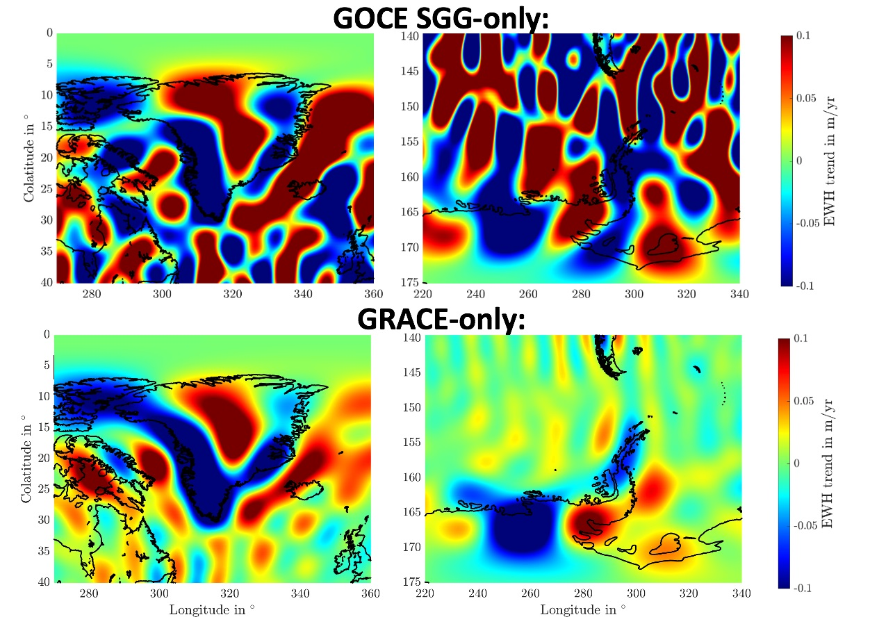
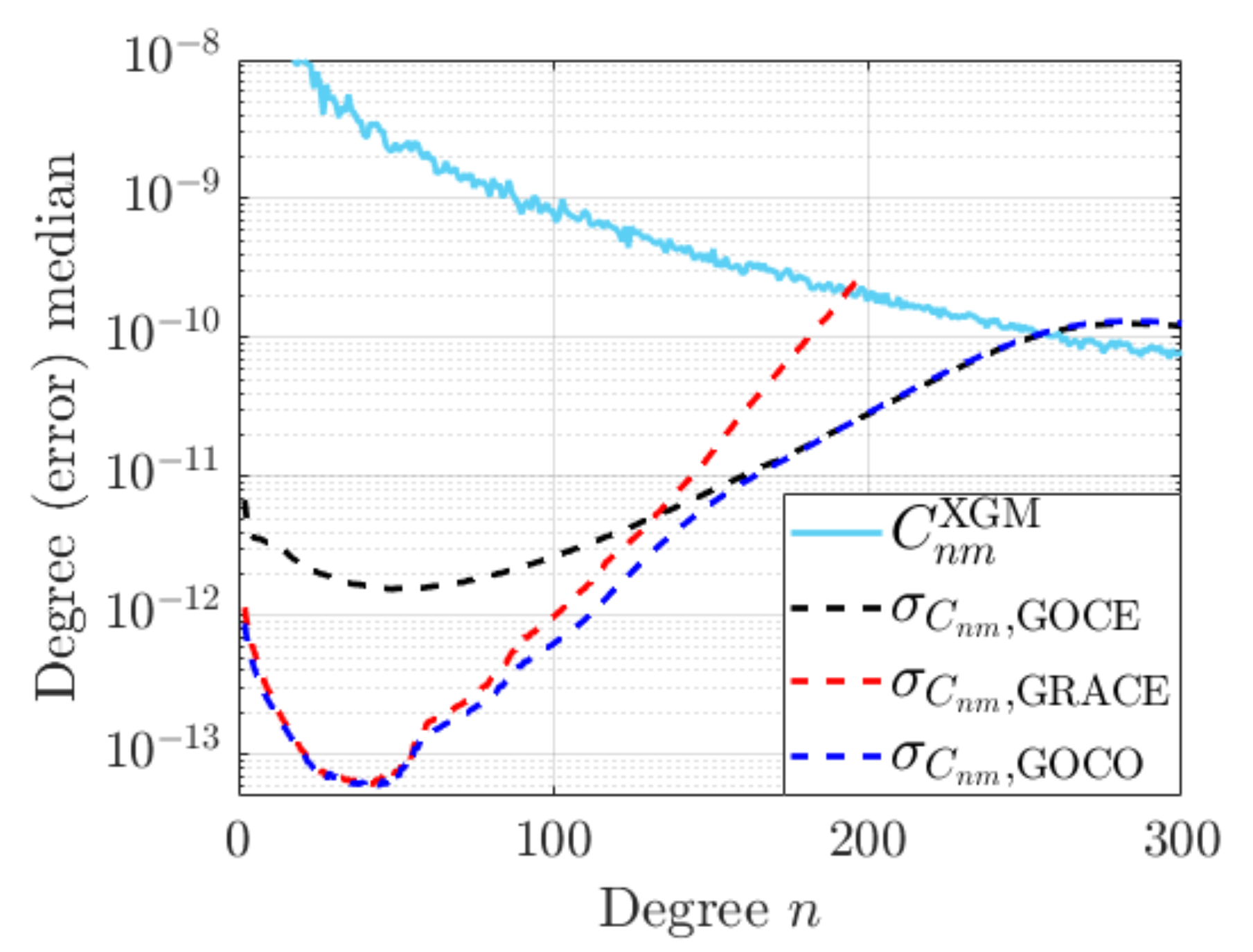
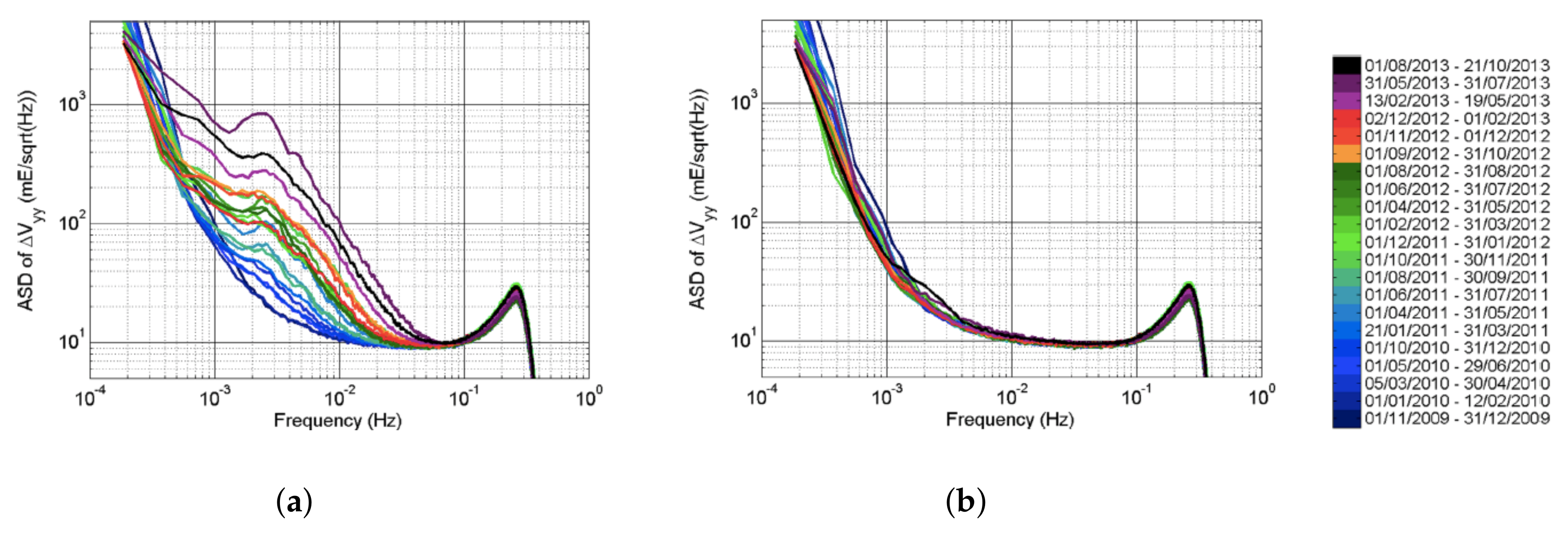
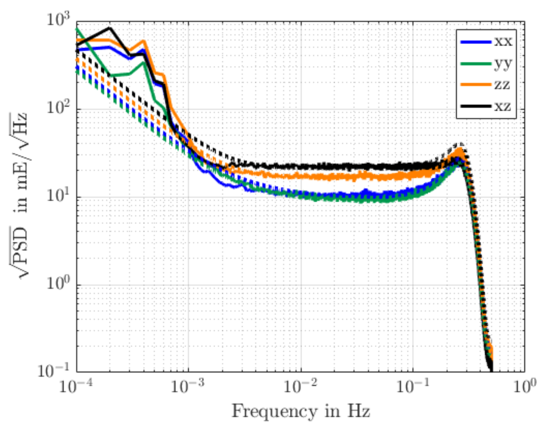
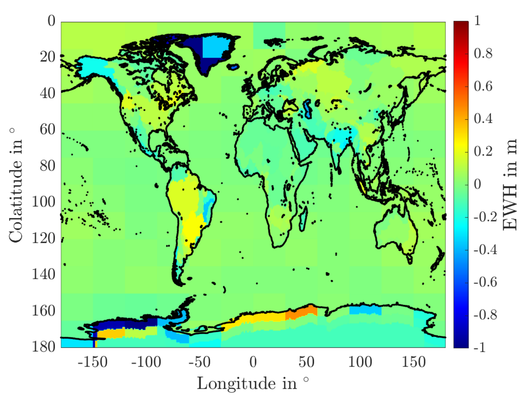
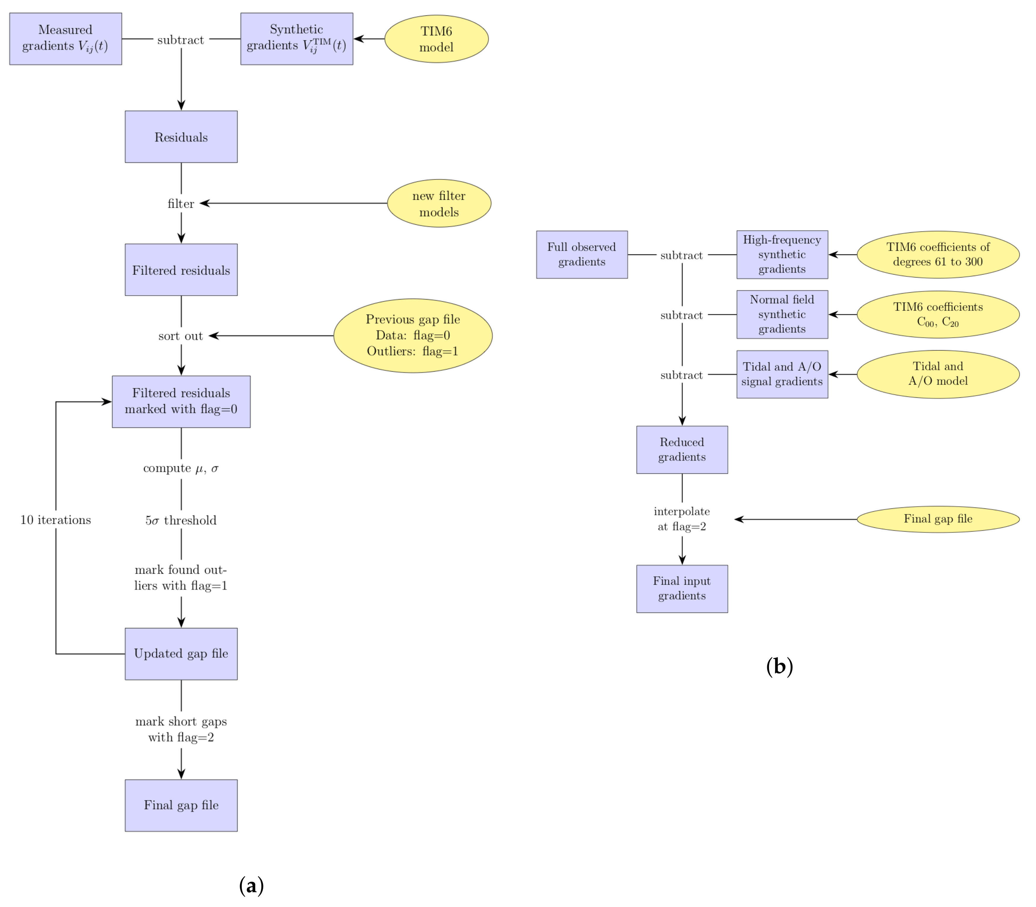
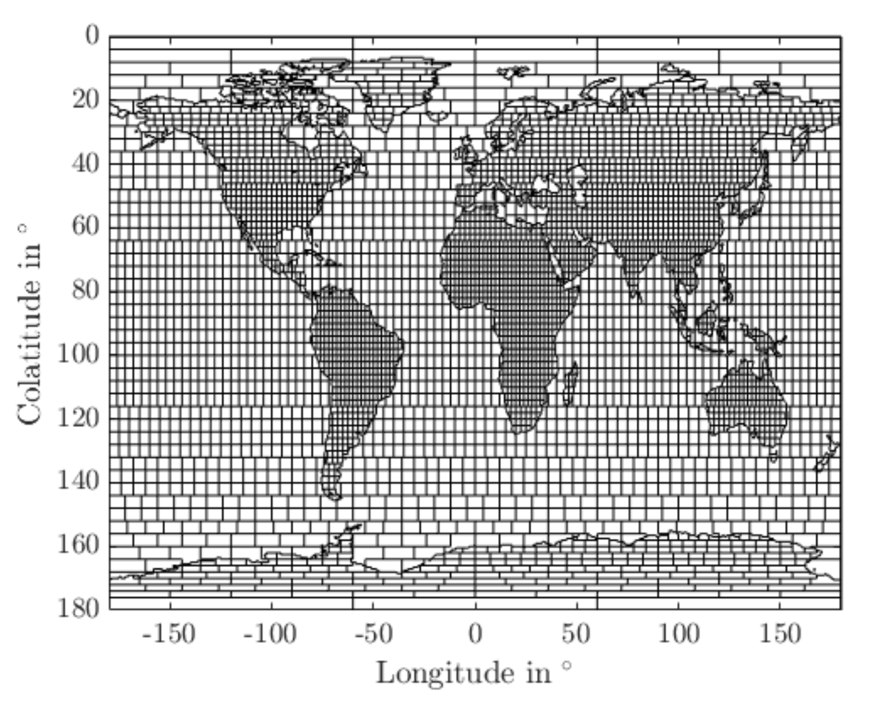
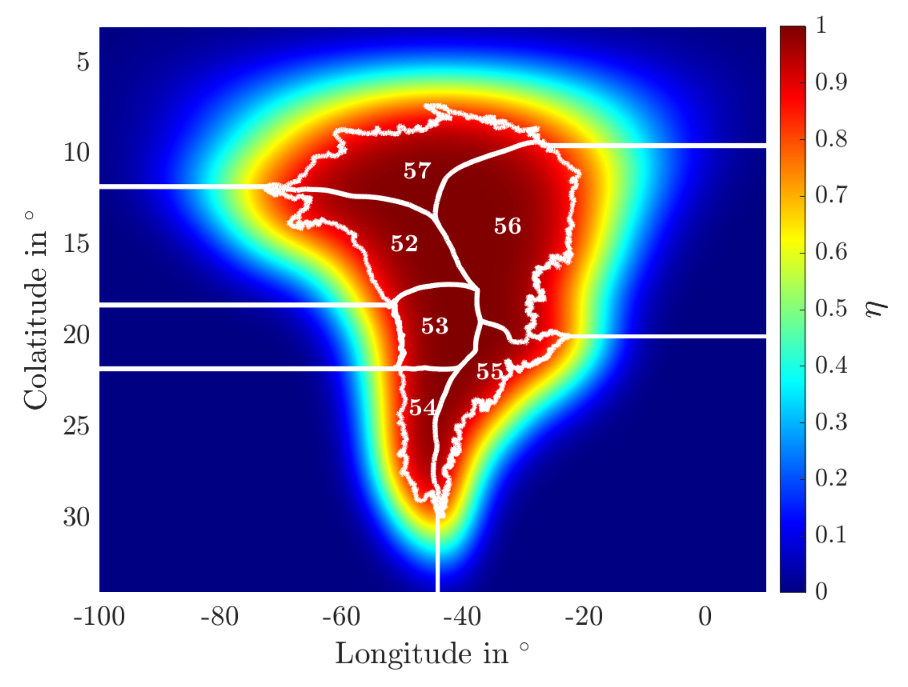
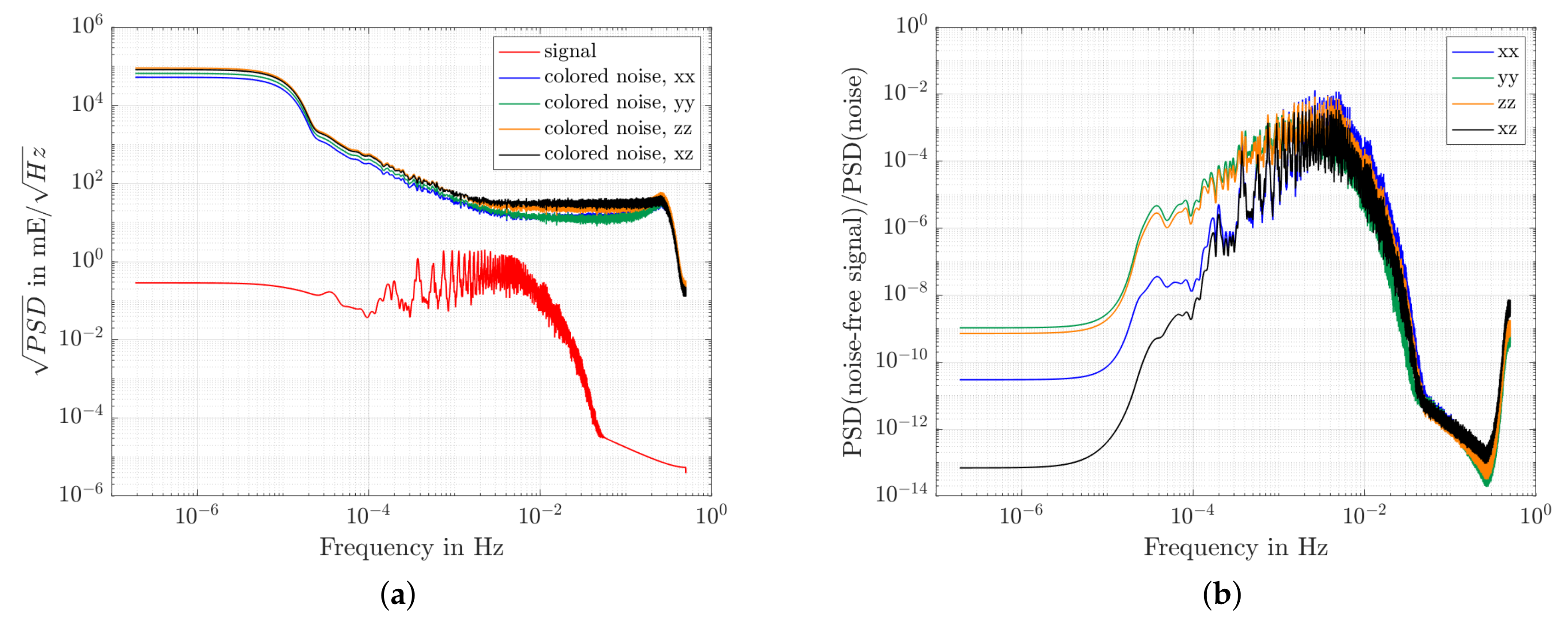
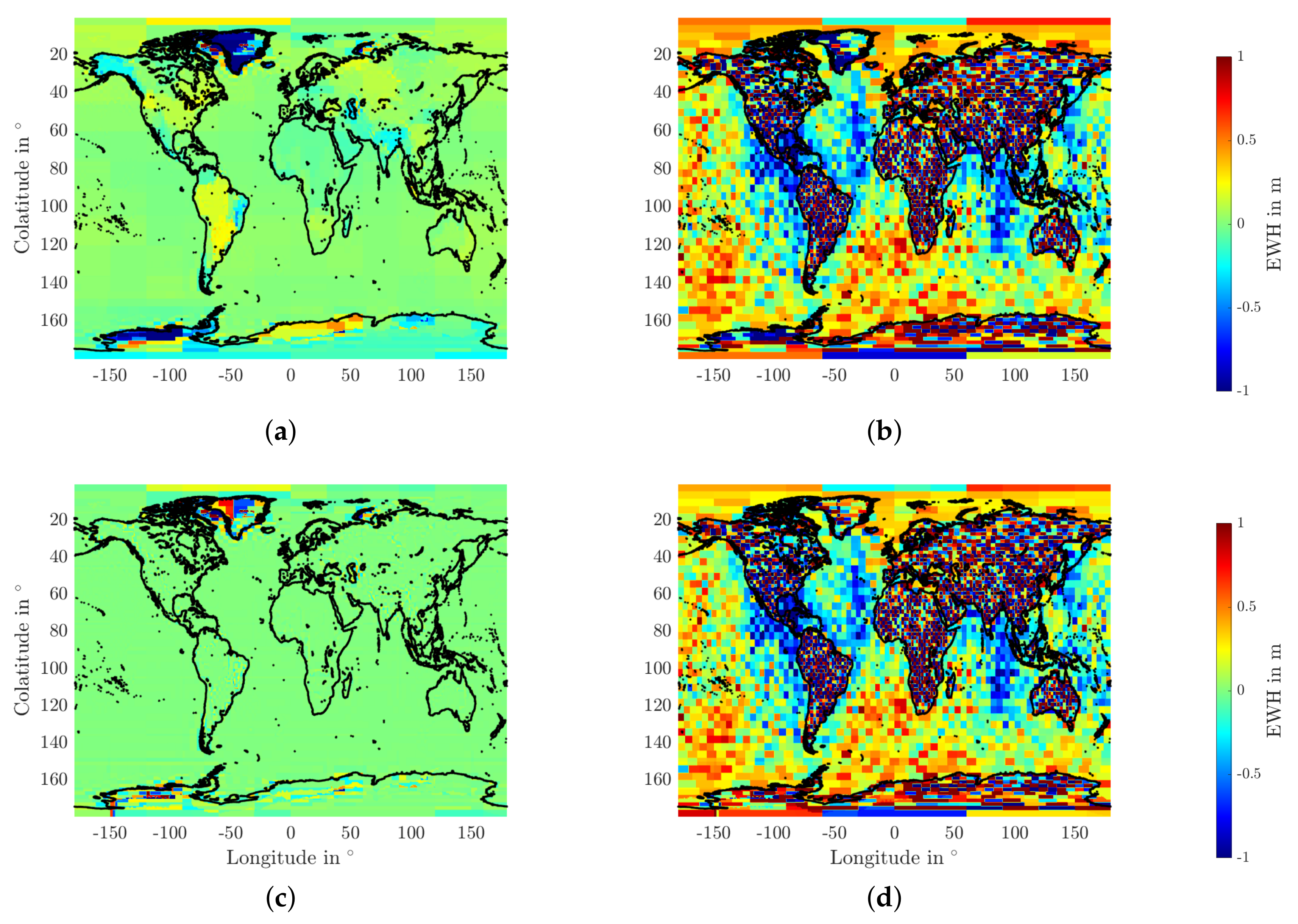
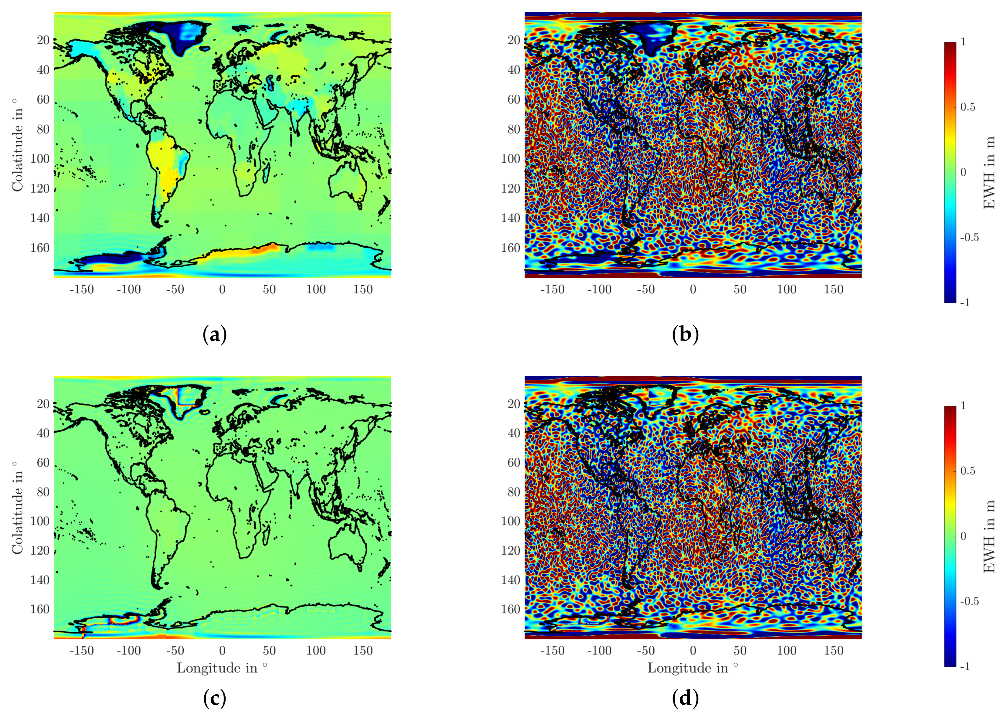
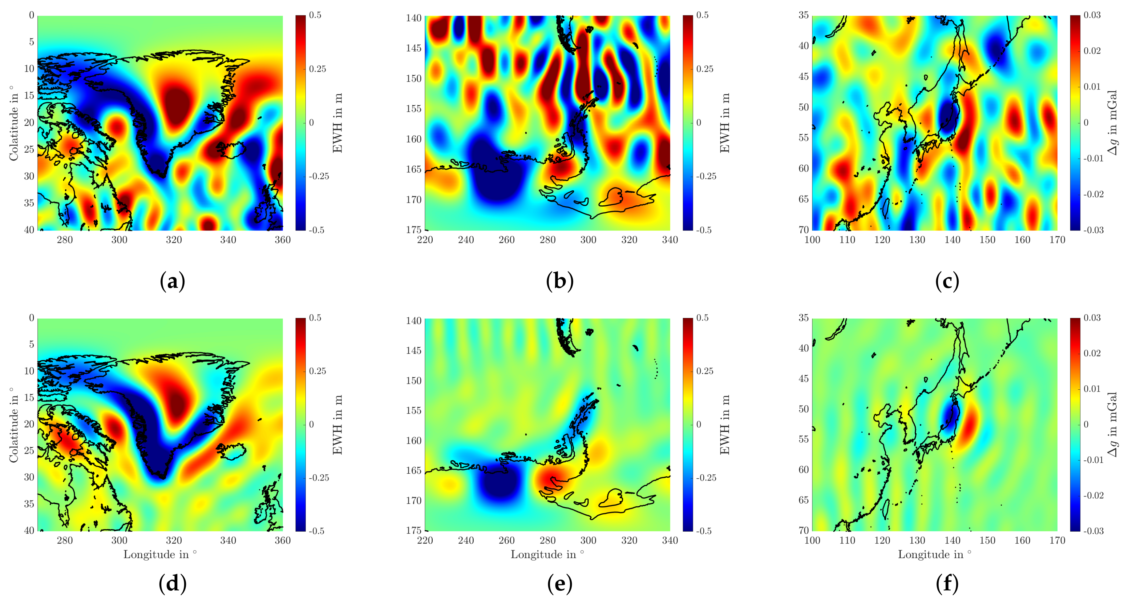
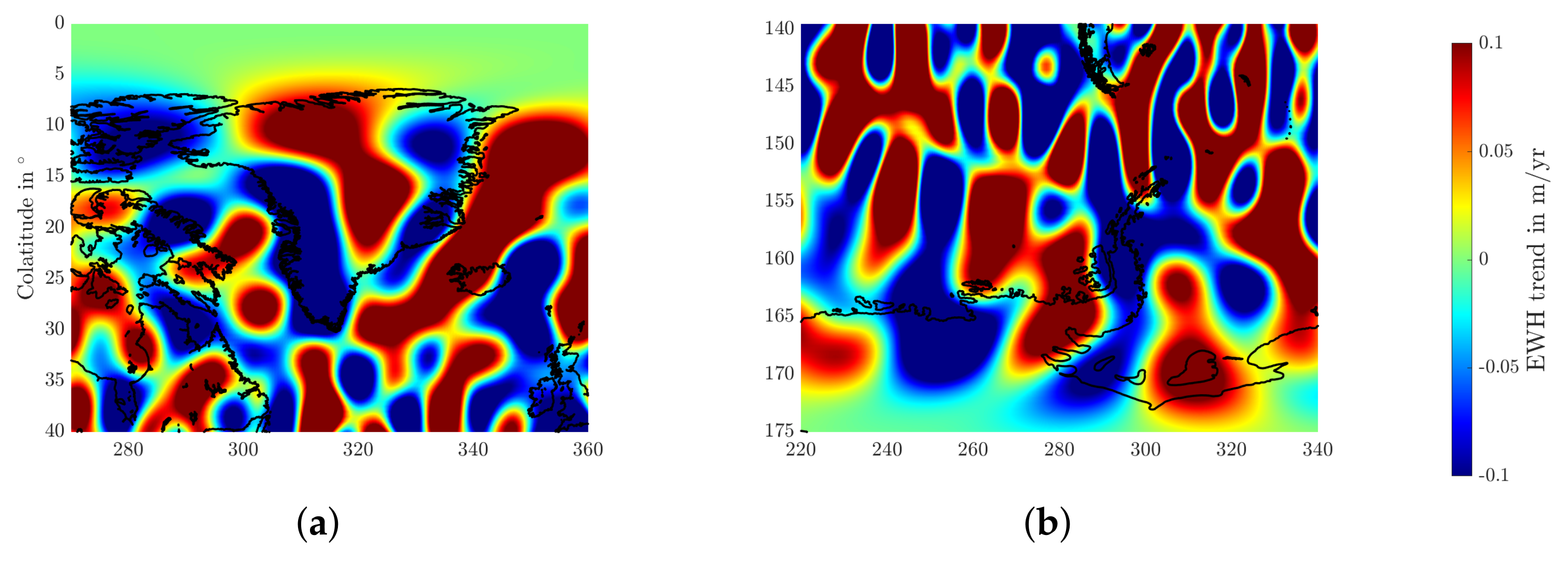
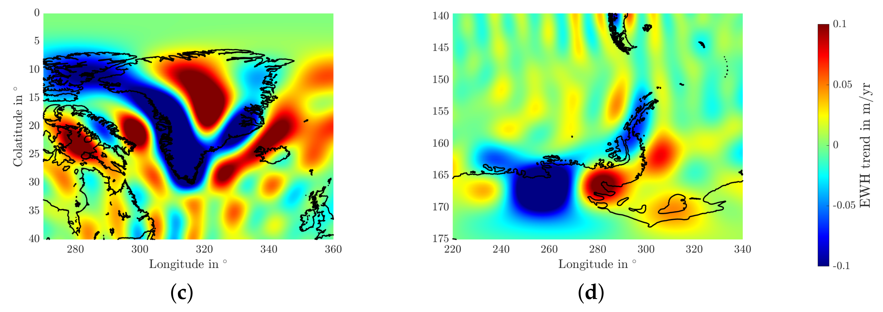
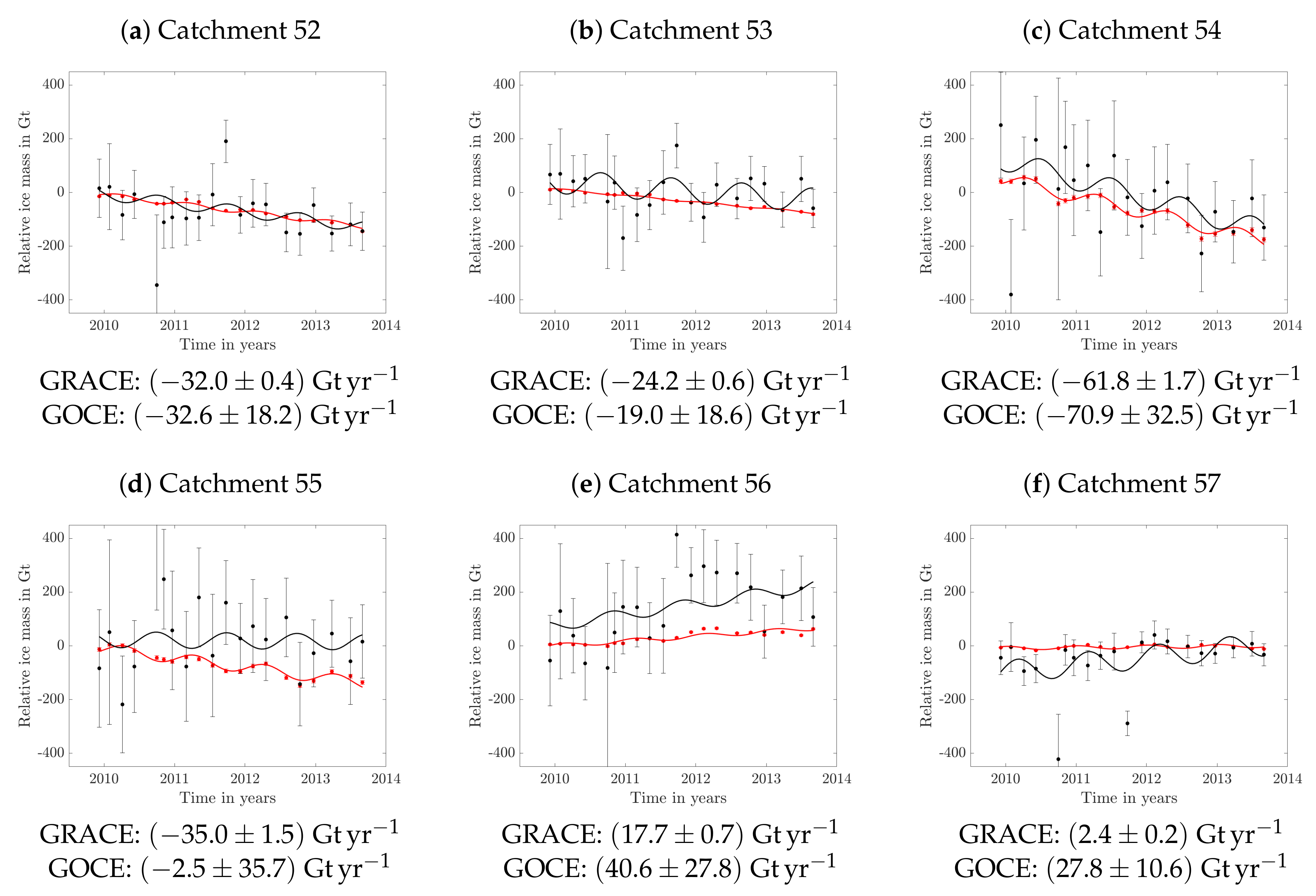
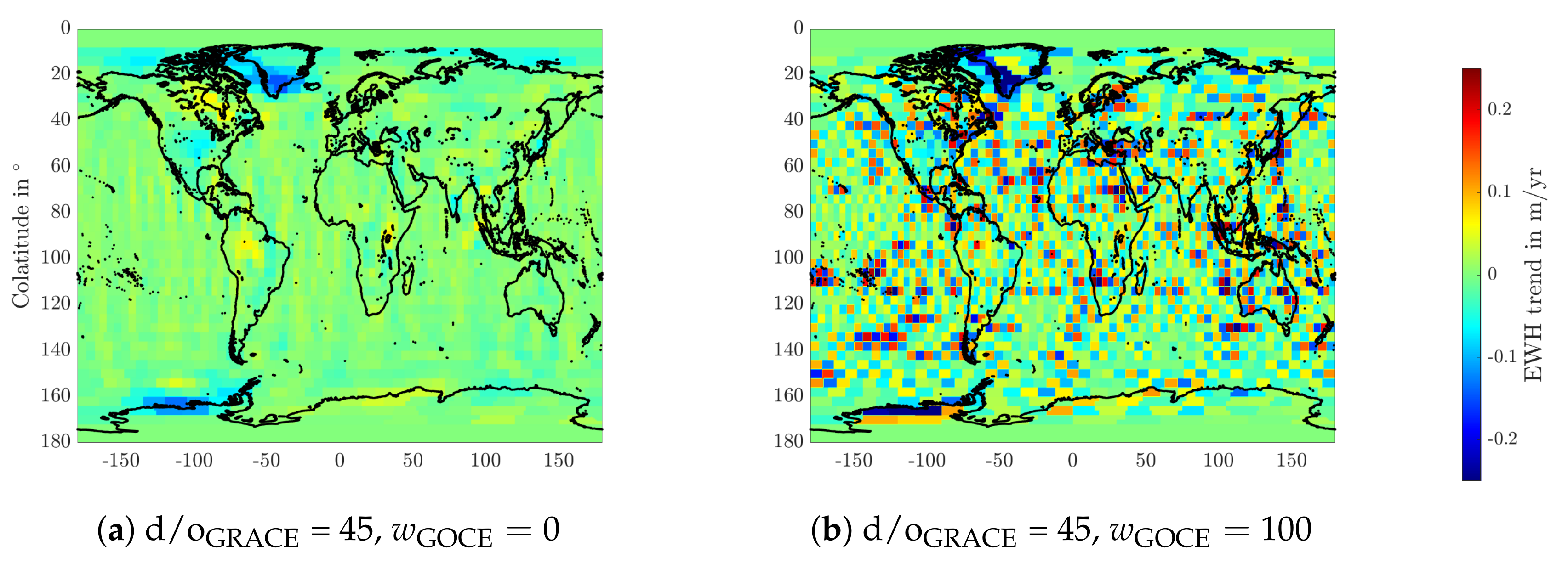
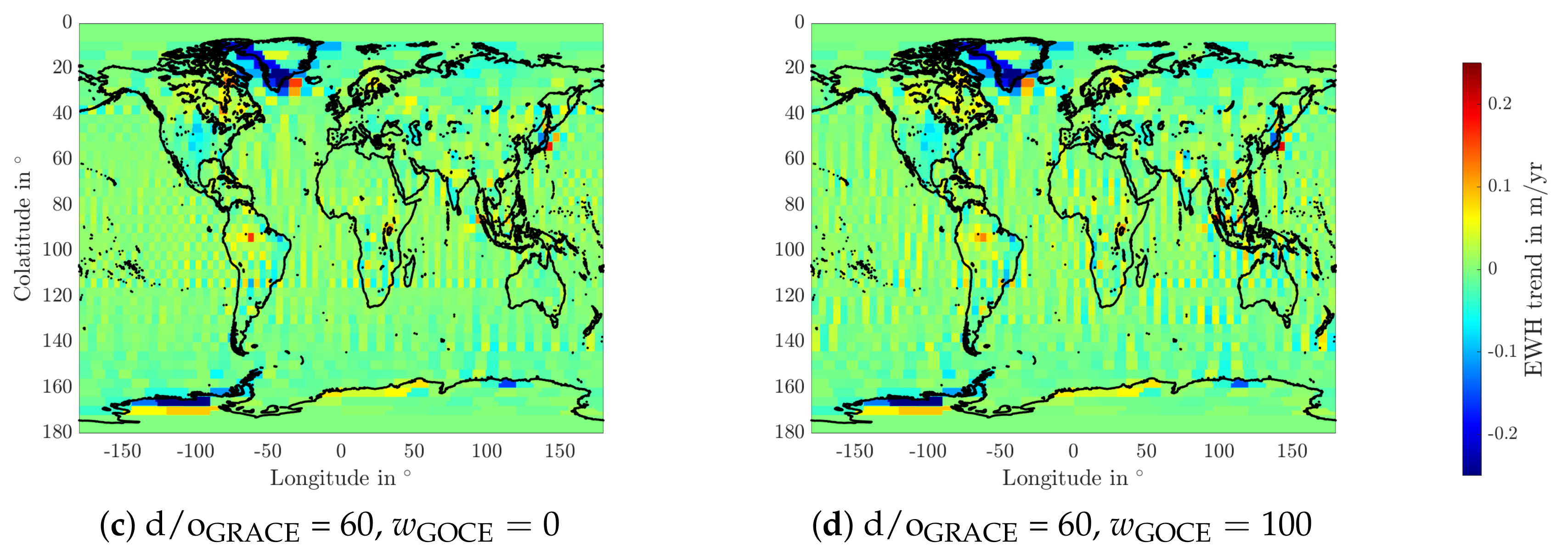
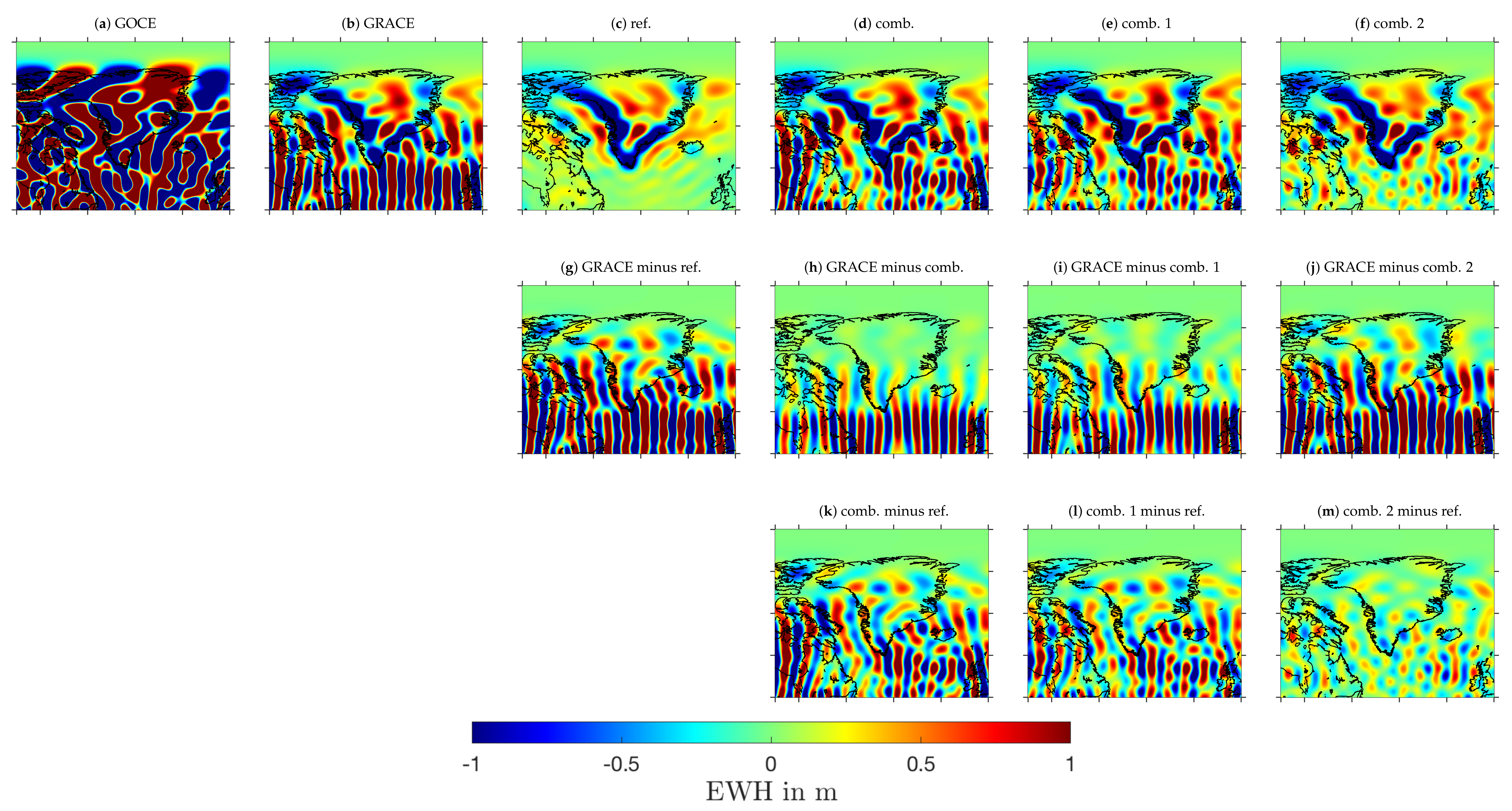
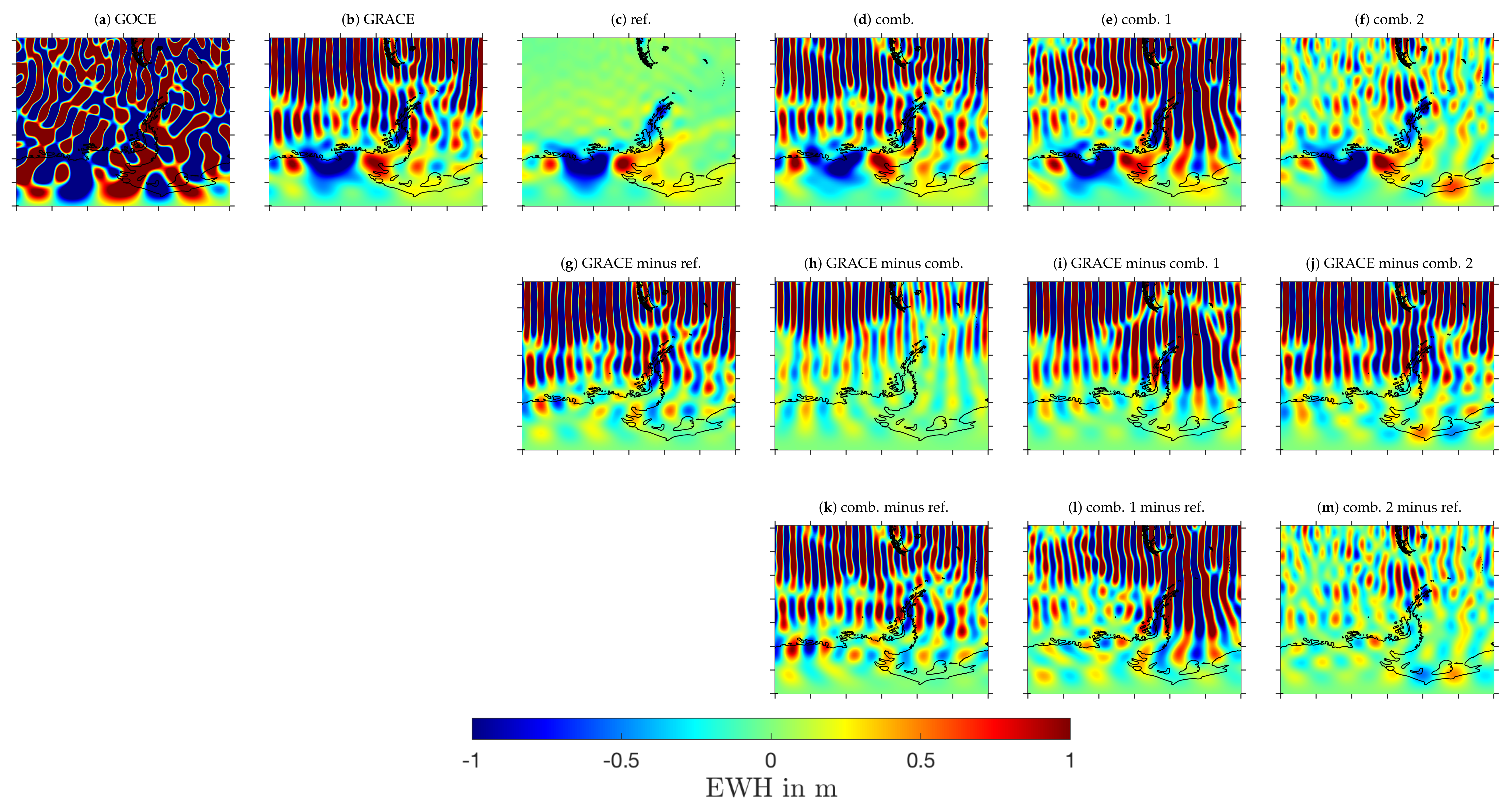
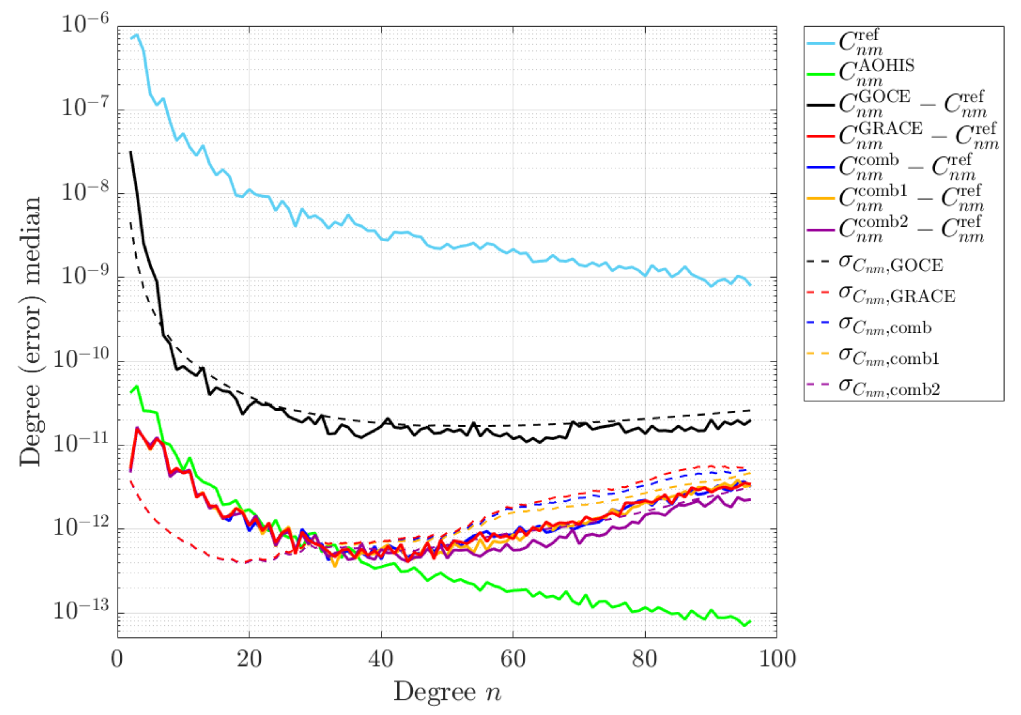
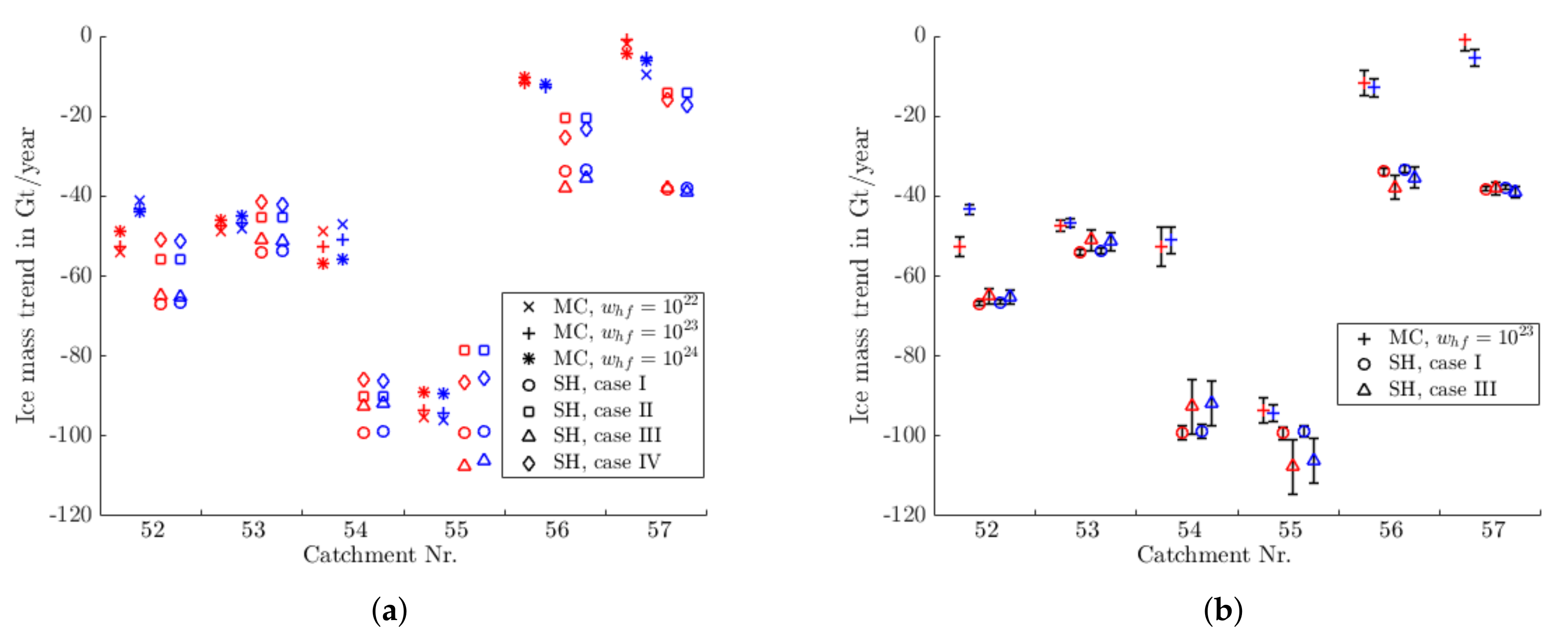
Table 1.
SH coefficient combinations defining the cases that are used to compute ice mass trends for the Greenland catchment areas based on SH gravity field models. and denote the minimum and maximum SH degrees of the coefficients included.
Table 1.
SH coefficient combinations defining the cases that are used to compute ice mass trends for the Greenland catchment areas based on SH gravity field models. and denote the minimum and maximum SH degrees of the coefficients included.
| Case | I | II | III | IV |
|---|---|---|---|---|
| 2 | 2 | 2 | 2 | |
| 60 | 60 | 96 | 96 | |
| coefficients of the polar gap wedge included | yes | no | yes | no |
Table 2.
Mass trend values obtained by the mascon (MC) and SH approaches for the six glacial catchment areas in Greenland (see Figure 7). Uncertainties are given as 1-sigma errors that are formally propagated from the variance-covariance matrices of the individual models. “GRACE” stands for GRACE-only results, “comb.” stands for results based on GRACE/GOCE SGG combination models, and denotes the relative difference of the GRACE and combination model-derived trend values (see Section 3.3.3). The meaning of the factor is explained in Section 2.2.5; SH cases I to IV are defined in Table 1. All trend values (GRACE, comb) are given in , is given in %.
| Catchment Nr. | 52 | 53 | 54 | 55 | 56 | 57 | |
|---|---|---|---|---|---|---|---|
| MC, | GRACE | ||||||
| comb. | |||||||
| 23.9 | 1.5 | 3.4 | −0.7 | −7.1 | −420.9 | ||
| MC, | GRACE | ||||||
| comb. | |||||||
| 17.8 | 1.5 | 2.8 | −0.7 | −10.9 | −642.9 | ||
| MC, | GRACE | ||||||
| comb. | |||||||
| 9.5 | 1.7 | 1.9 | −0.6 | −18.8 | −38.9 | ||
| SH, case I | GRACE | ||||||
| comb. | |||||||
| 0.5 | 0.5 | 0.3 | 0.4 | 1.4 | 1.1 | ||
| SH, case II | GRACE | ||||||
| comb. | |||||||
| −0.05 | 0.1 | 0.06 | 0.01 | −0.5 | −0.3 | ||
| SH, case III | GRACE | ||||||
| comb. | |||||||
| −0.4 | −0.6 | 0.9 | 1.4 | 6.6 | −2.2 | ||
| SH, case IV | GRACE | ||||||
| comb. | |||||||
| −0.3 | −1.5 | −0.6 | 1.2 | 8.3 | −7.5 |
Publisher’s Note: MDPI stays neutral with regard to jurisdictional claims in published maps and institutional affiliations. |
© 2020 by the authors. Licensee MDPI, Basel, Switzerland. This article is an open access article distributed under the terms and conditions of the Creative Commons Attribution (CC BY) license (http://creativecommons.org/licenses/by/4.0/).
Share and Cite
MDPI and ACS Style
Heller, B.; Siegismund, F.; Pail, R.; Gruber, T.; Haagmans, R. Temporal Gravity Signals in Reprocessed GOCE Gravitational Gradients. Remote Sens. 2020, 12, 3483. https://0-doi-org.brum.beds.ac.uk/10.3390/rs12213483
AMA Style
Heller B, Siegismund F, Pail R, Gruber T, Haagmans R. Temporal Gravity Signals in Reprocessed GOCE Gravitational Gradients. Remote Sensing. 2020; 12(21):3483. https://0-doi-org.brum.beds.ac.uk/10.3390/rs12213483
Chicago/Turabian StyleHeller, Betty, Frank Siegismund, Roland Pail, Thomas Gruber, and Roger Haagmans. 2020. "Temporal Gravity Signals in Reprocessed GOCE Gravitational Gradients" Remote Sensing 12, no. 21: 3483. https://0-doi-org.brum.beds.ac.uk/10.3390/rs12213483
Note that from the first issue of 2016, this journal uses article numbers instead of page numbers. See further details here.