Validation of Sentinel-3 OLCI Integrated Water Vapor Products Using Regional GNSS Measurements in Crete, Greece


Abstract
:1. Introduction
2. Methodology and Dataset
2.1. Estimation of the IWV from OLCI
2.2. Estimation of the IWV from GNSS Measurements
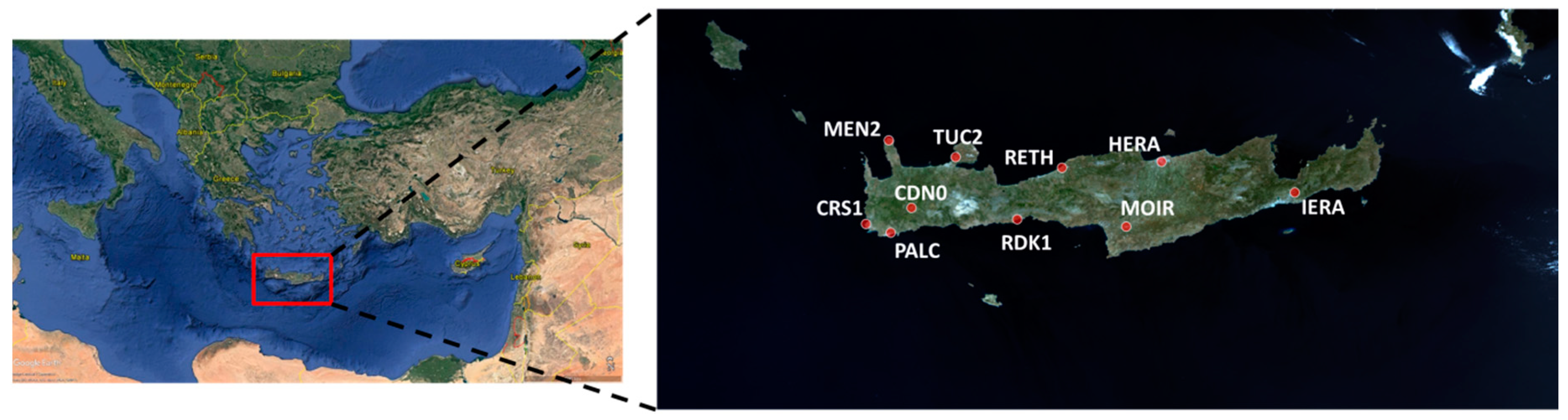
2.3. The Regional GNSS Monitoring Network
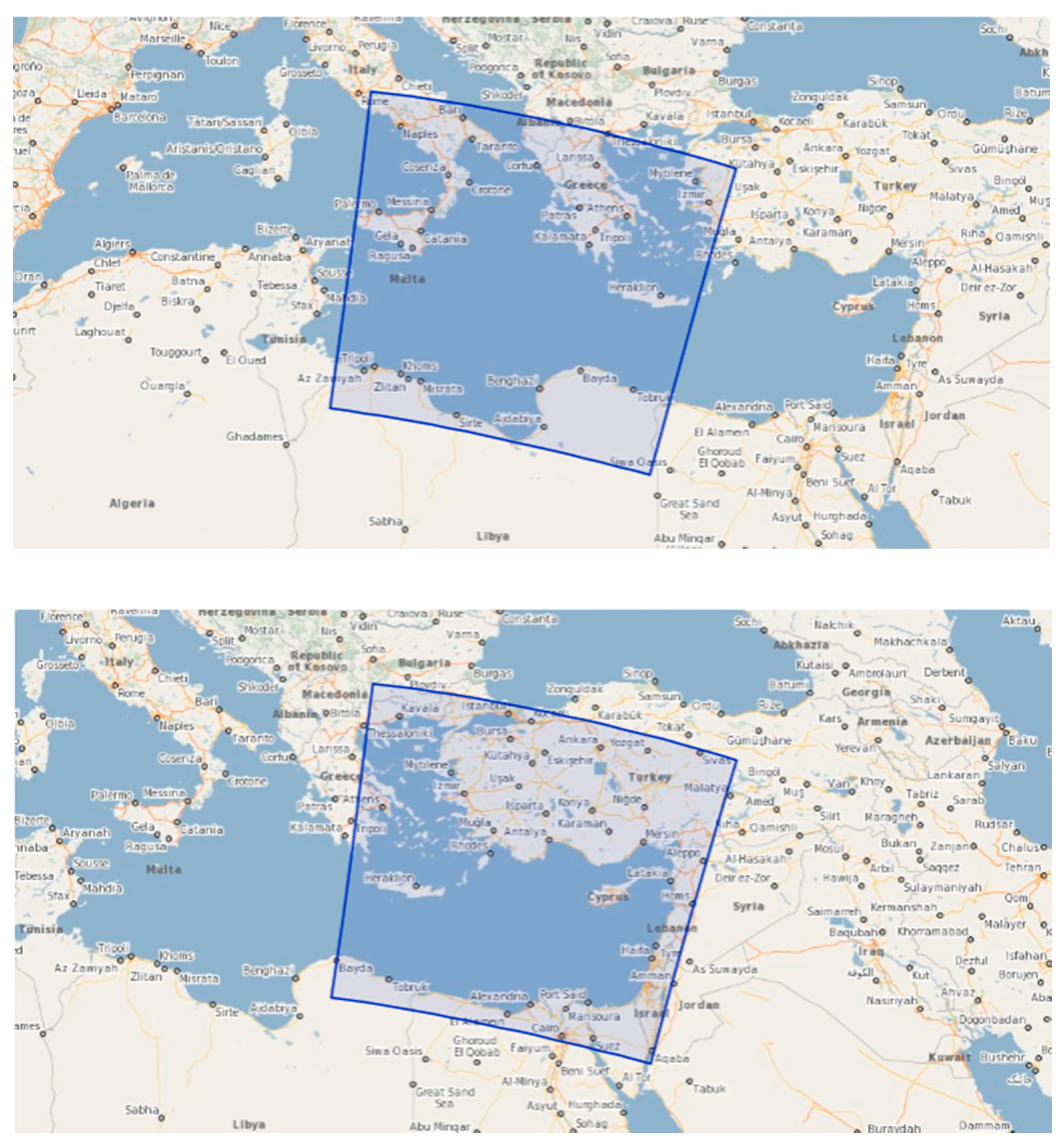
2.4. The OLCI Dataset
3. Results
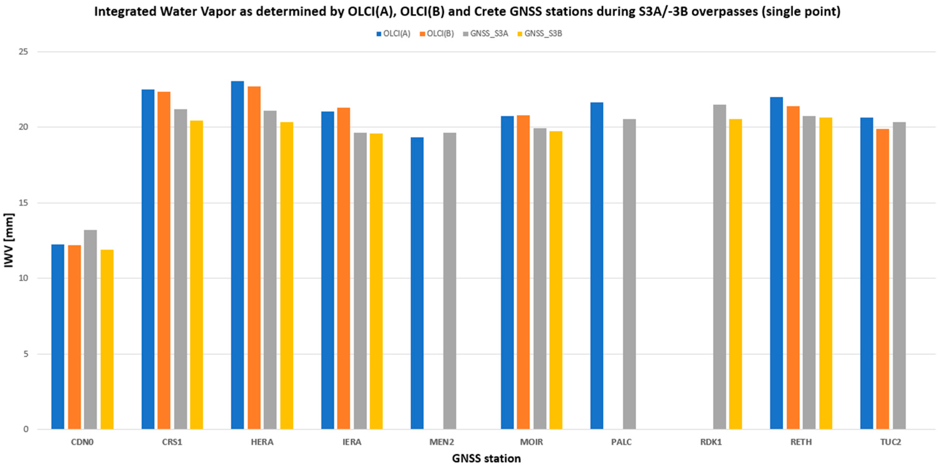
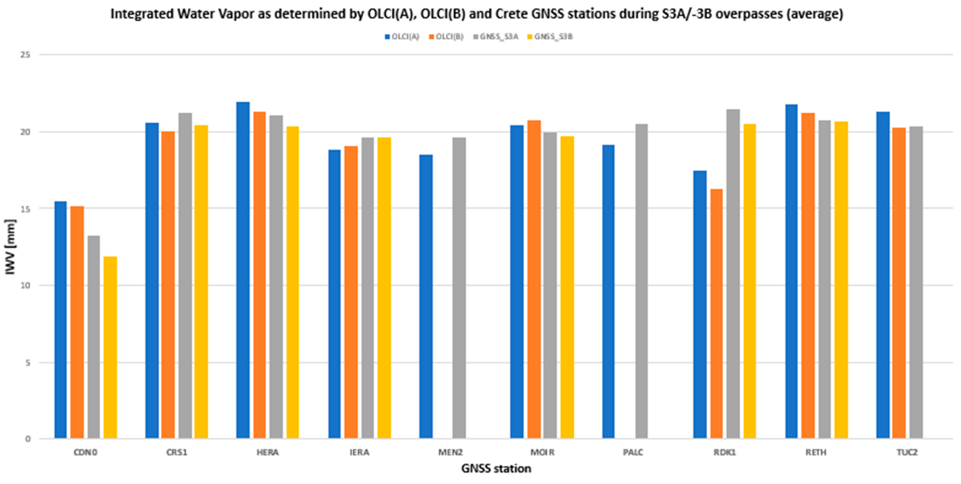
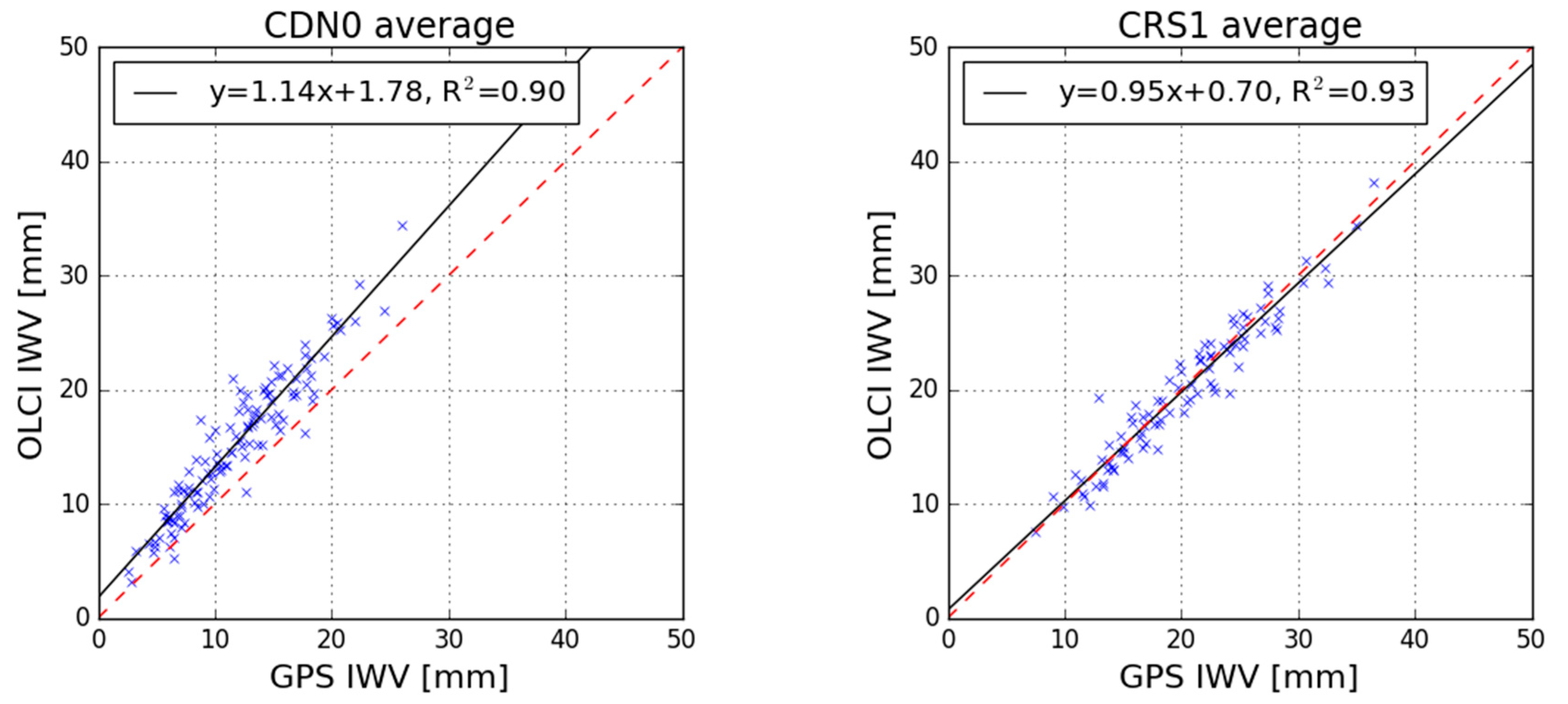
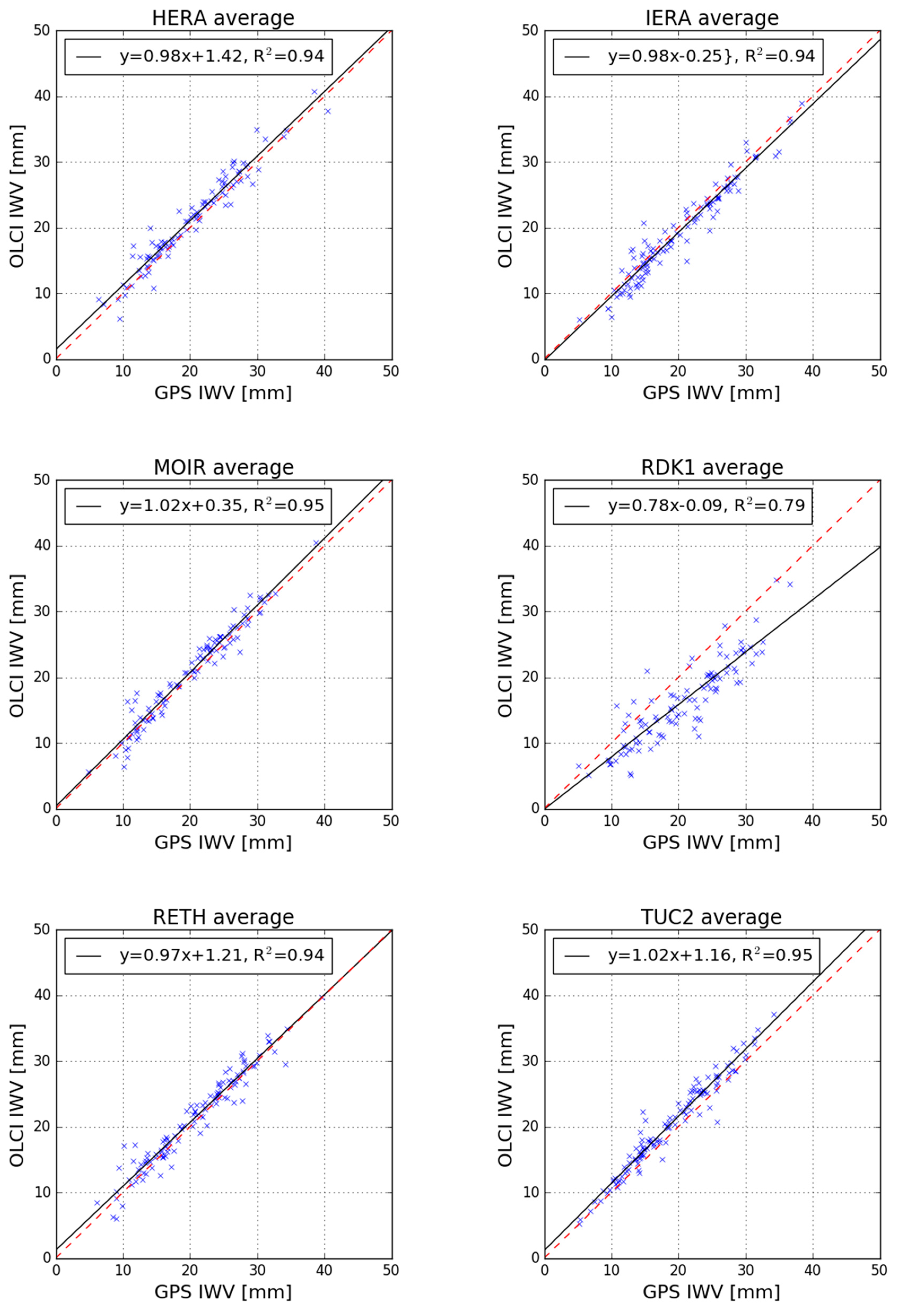
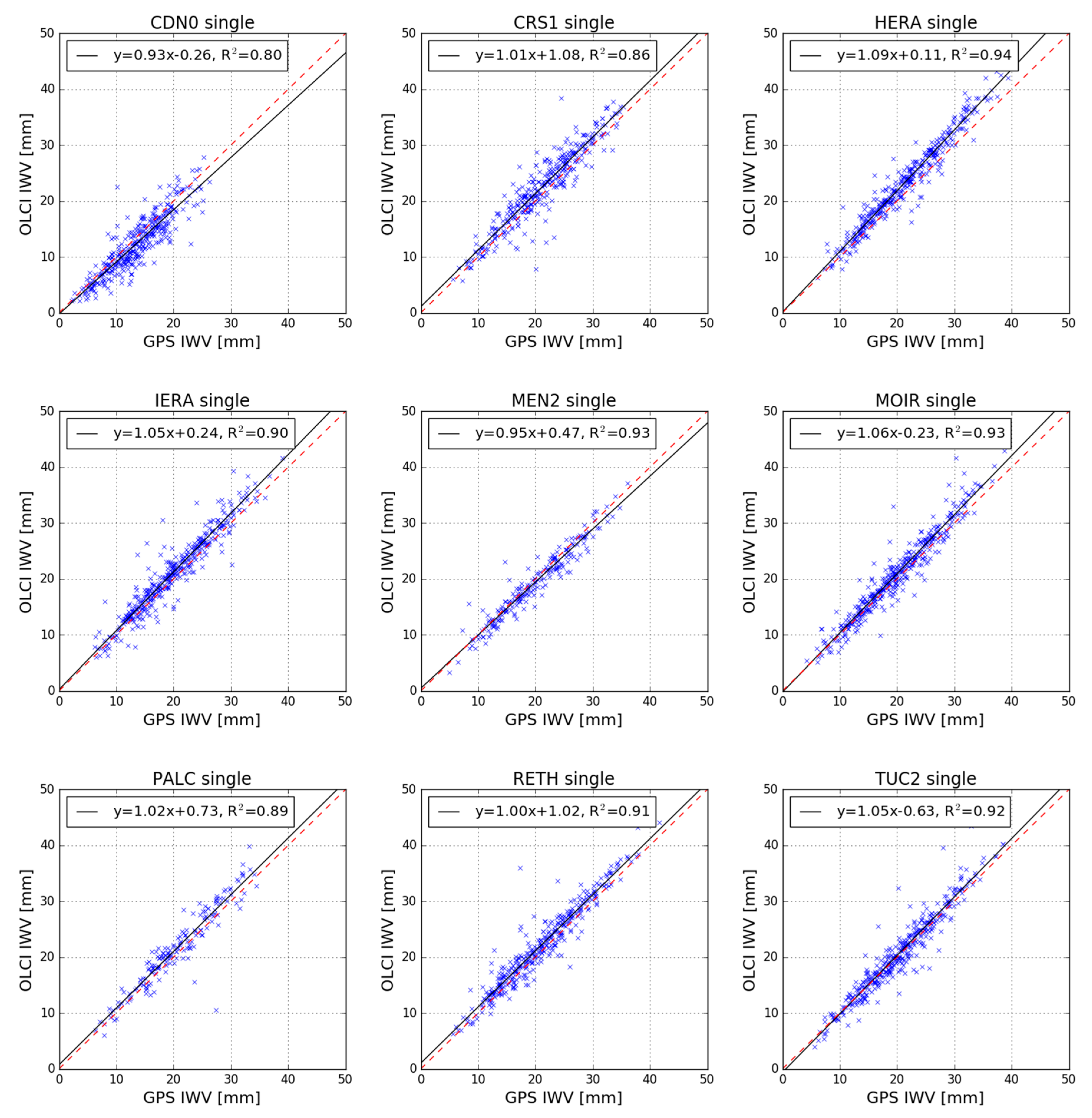
3.1. Absolute Bias of Sentinel-3 OLCI IWV Products
- The mean bias of OLCI(A) is determined as +0.57 mm and −0.23 mm implementing the “single point” and the “area of influence” approach respectively and using data covering a 4-year operational period;
- The mean bias of OLCI(B) is determined as +1.07 mm and +0.24 mm implementing the “single point” and the “area of influence” approach respectively, over a one-year period of validation data;
- The magnitude of OLCI(A) and OLCI(B) bias is within the operational capabilities of the satellite instrument but also the accuracy of GNSS-derived IWV values that have been used as reference in this study;
- The OLCI and GNSS IWV values are significantly correlated irrespectively of validation sites and approach used.
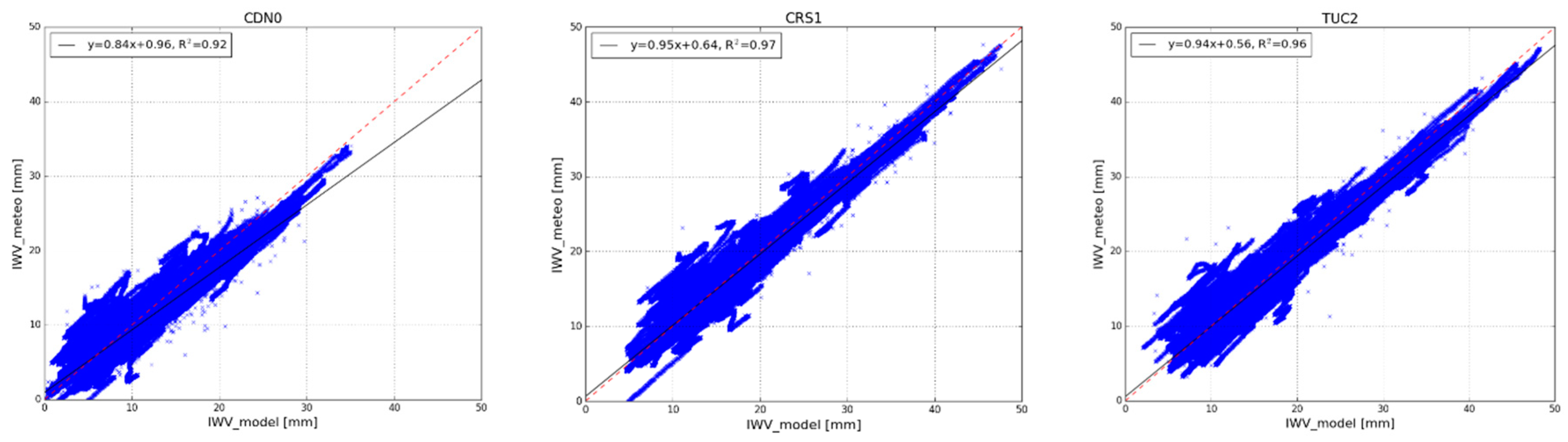
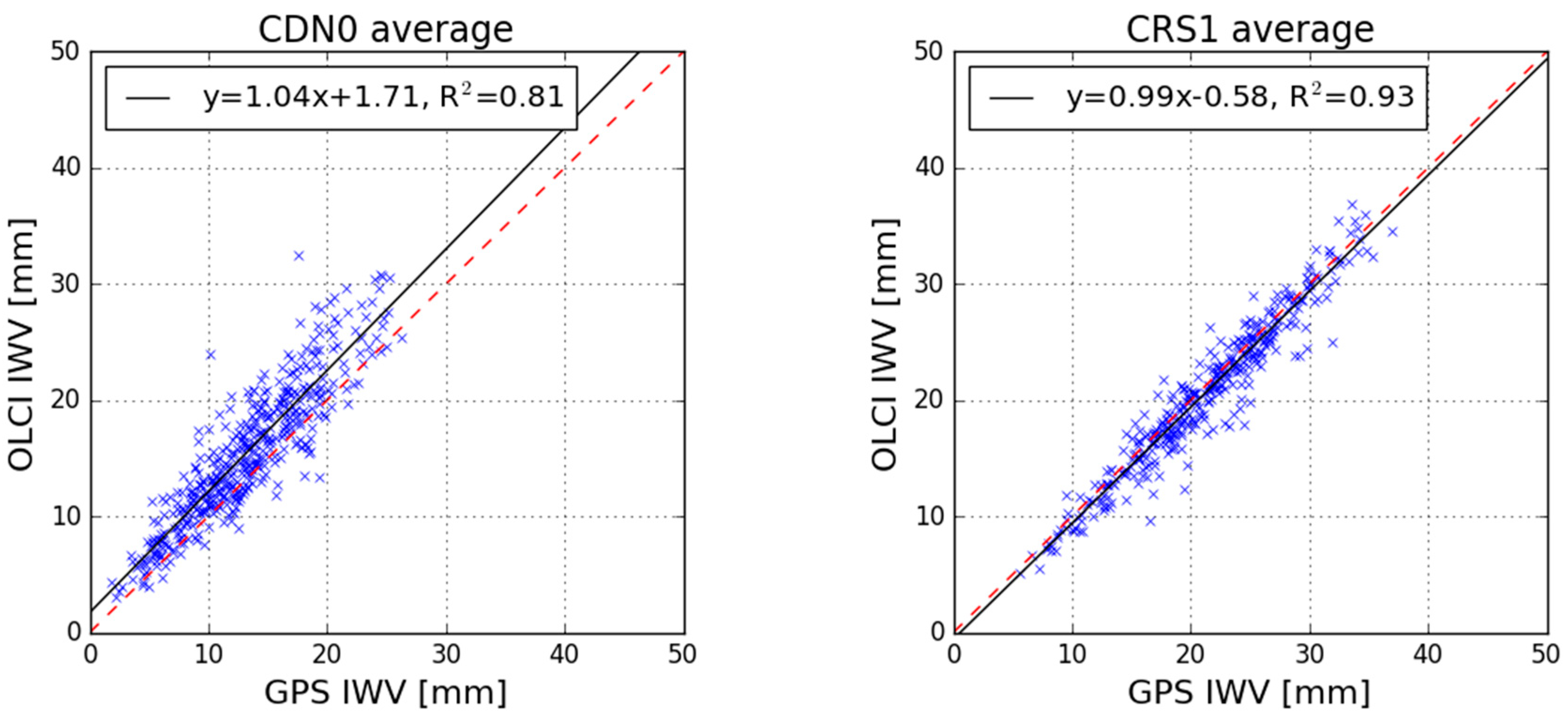
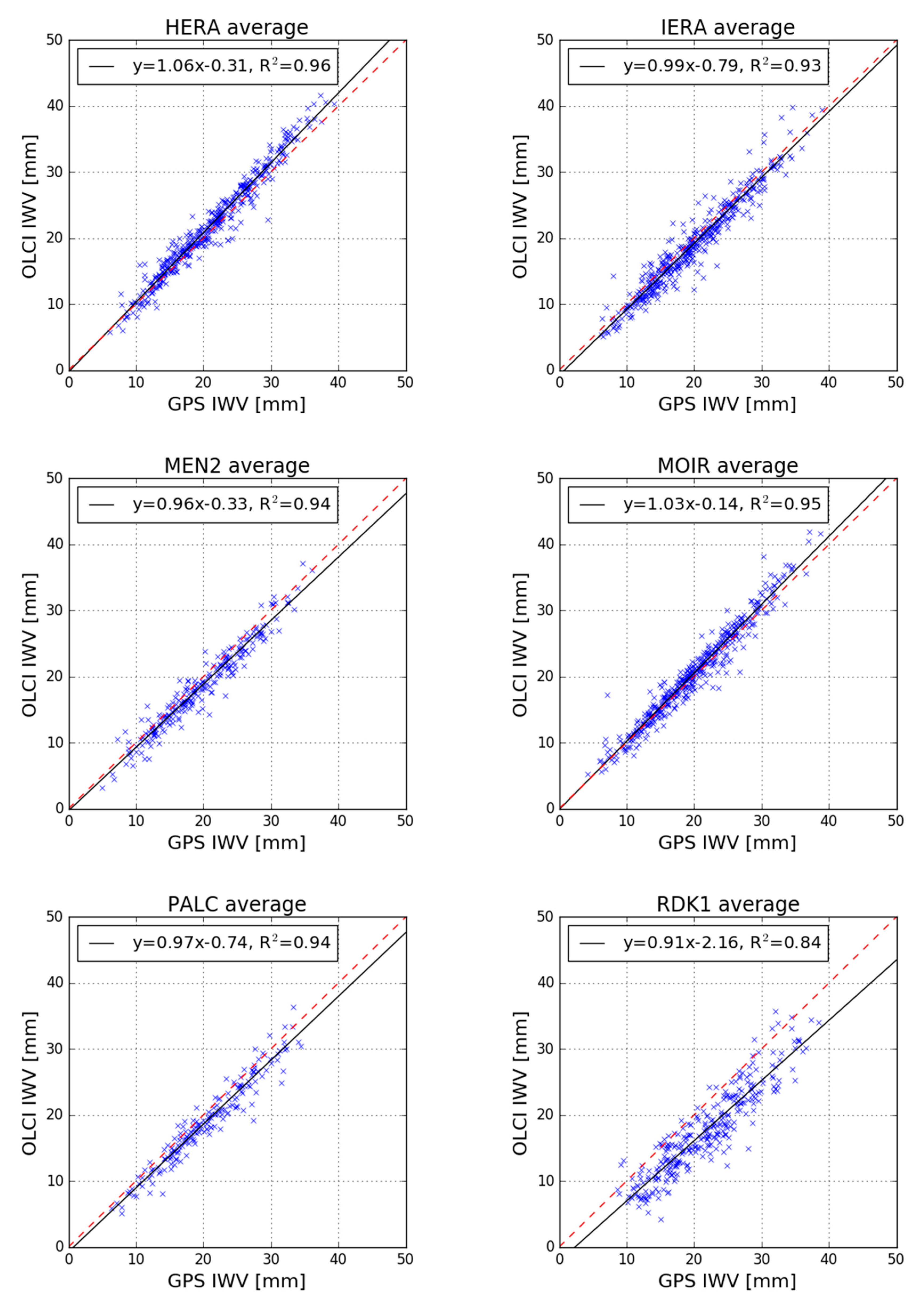
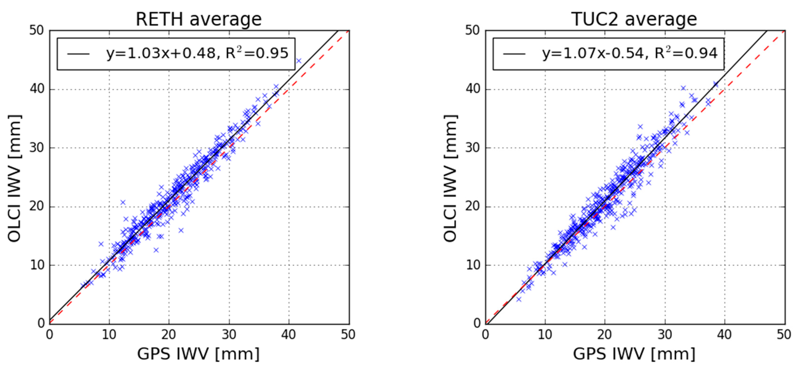
3.2. Relative Bias of Sentinel-3 OLCI IWV Products
4. Discussion
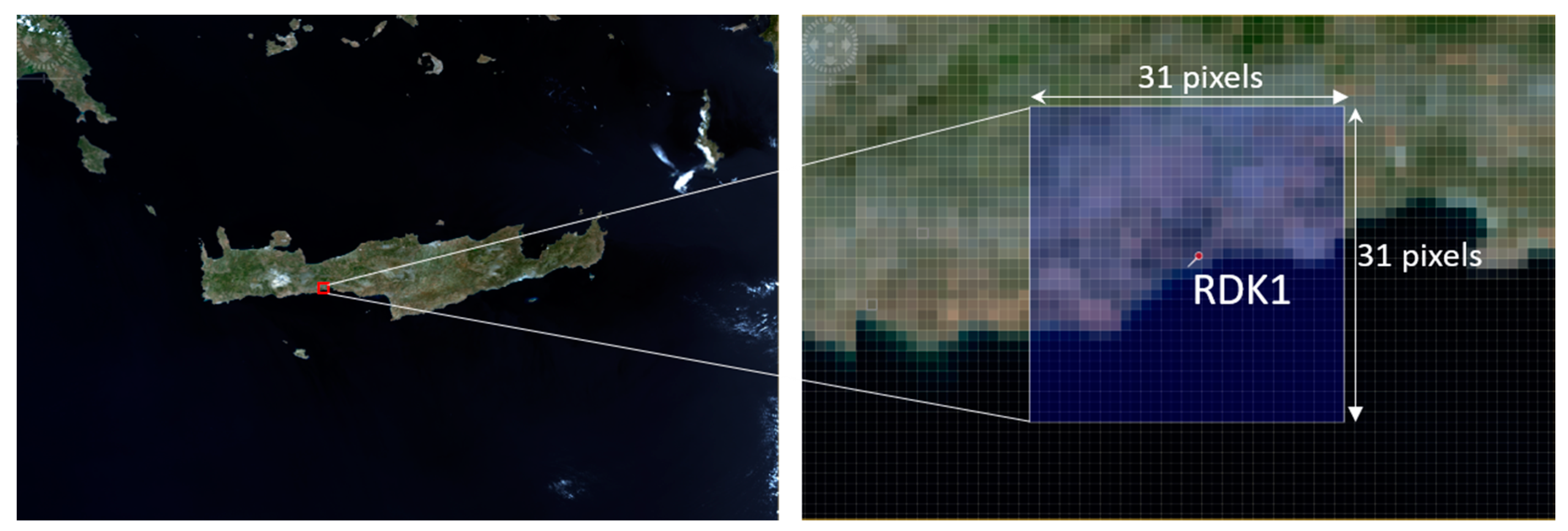
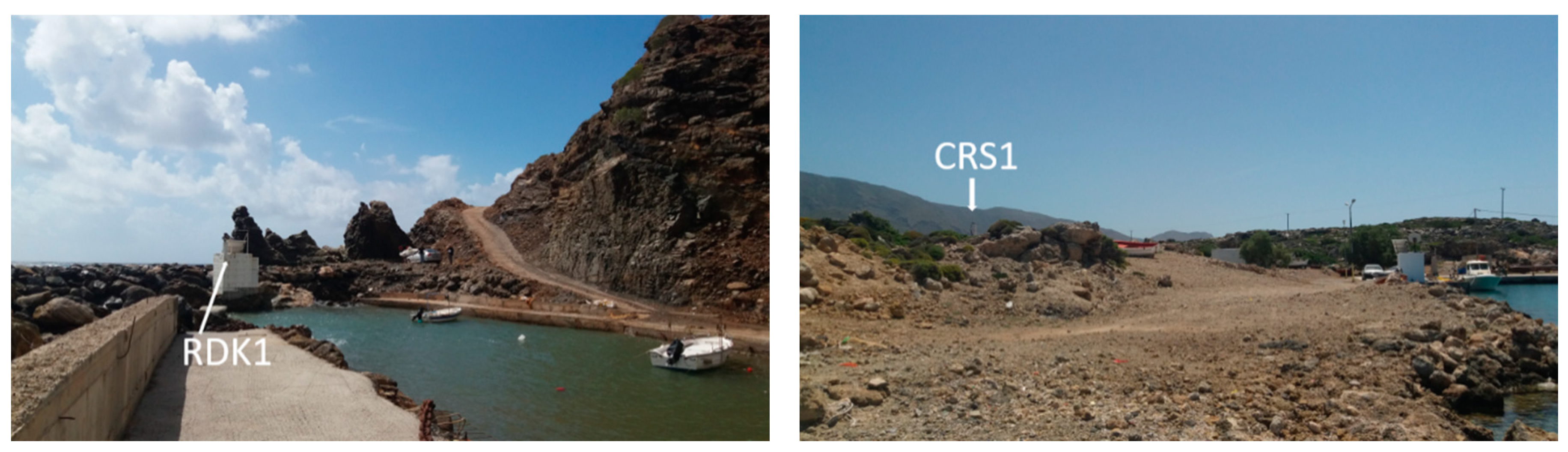
- The OLCI pixel that contains the RDK1 station is flagged as “WATER”. Thus, it is expected that the OLCI IWV retrieval algorithm will not perform well at this location. Even though implementation of the “area of influence” approach resolved this problem and made it possible to obtain valid OLCI IWV values in the vicinity of the RDK1 station, the RDK1 site presents the largest deviation among all examined GNSS stations. A few explanations for this deviation are possible: The geometry of the GPS satellites is worse (weak) compared to other GNSS sites, as high mountains in the North (see Figure 7) block the signal reception from satellites in that direction. This may be resolved if a multi-constellation (i.e., GPS, GLONASS and Galileo) receiver is operated at this location. Another possible explanation is the absence of in-situ meteorological sensor. That entails that the applied VMF1 model does not perform well in the RDK1 area and cannot sense the particularities that the specific geomorphology causes to the water vapor.
- Two alternative techniques have been employed to determine the OLCI IWV value at a GNSS station location. Through the “area of influence” approach, it was possible to derive valid OLCI IWV values, even when the single OLCI pixel nearest to the GNSS station produced invalid IWV values. This is a valuable outcome when monitoring the OLCI IWV performance in coastal regions. The results presented in Table 3 and Table 5 cannot help us arrive at a definite conclusion on the performance of each approach. In the cases of CDN0 and TUC2 (land only stations), the “area of influence” approach produces largest IWV values than the “single point” approach. The opposite stands true for the rest of the GNSS stations. The difference between the IWV values is within ±3 mm by these two approaches.
- At present, there is no “golden rule” for defining a representative size for the area of influence in the IWV value. The actual size of the “area of influence” varies both spatially and temporally and depends on local conditions. In this work, we have chosen to use an area of 9.3 km2, which is close to the size of 10 km2 applied in [41]. This size of 9.3 km2 has been selected in our case to compare both results directly from the two studies. Nevertheless, a more detailed and independent investigation on the effective area of influence of GNSS water vapor products is needed to be carried out in the future.
- The number of validation points to be used for the comparison analysis affects the reliability and the conclusions drawn out of a statistical analysis. Even though the results presented in this study are statistically significant (good p-value, adequate number of sampling points), a compromise to the quality of the IWV values may have been made. For example, when the “area of influence” approach was employed, the percentage of valid pixels within each window of the OLCI image has not been taken into consideration. This was made intentionally to enlarge the number of valid OLCI-GNSS sampling points for validation. Using stricter criteria (i.e., exclude an OLCI image window if it has less than 50% of its pixels flagged as “LAND”, within the area of influence) would significantly reduce the number of validation points. Note that the global analysis carried out in [41] used only 5% of the total available products for their validation.
- The continuous operation of the GNSS stations is a vital requirement for carrying out an effective validation. Because it has to be ensured that whenever a valid OLCI image is captured, there will be always ground measurements available to compare. In some cases, improper operation of GNSS stations limited comparison affecting the total number of validation points. Also, collocation of the GNSS stations with meteorological stations reduces the possibility of reverting to global models for the estimation of the atmospheric pressure.
5. Conclusions
Author Contributions
Funding
Acknowledgments
Conflicts of Interest
Appendix A

| Site | Lat (Deg) | Long (Deg) | Ell.Height (m) | VN (m/yr) | VE (m/yr) | VU (m/yr) | Time Span (Years) |
|---|---|---|---|---|---|---|---|
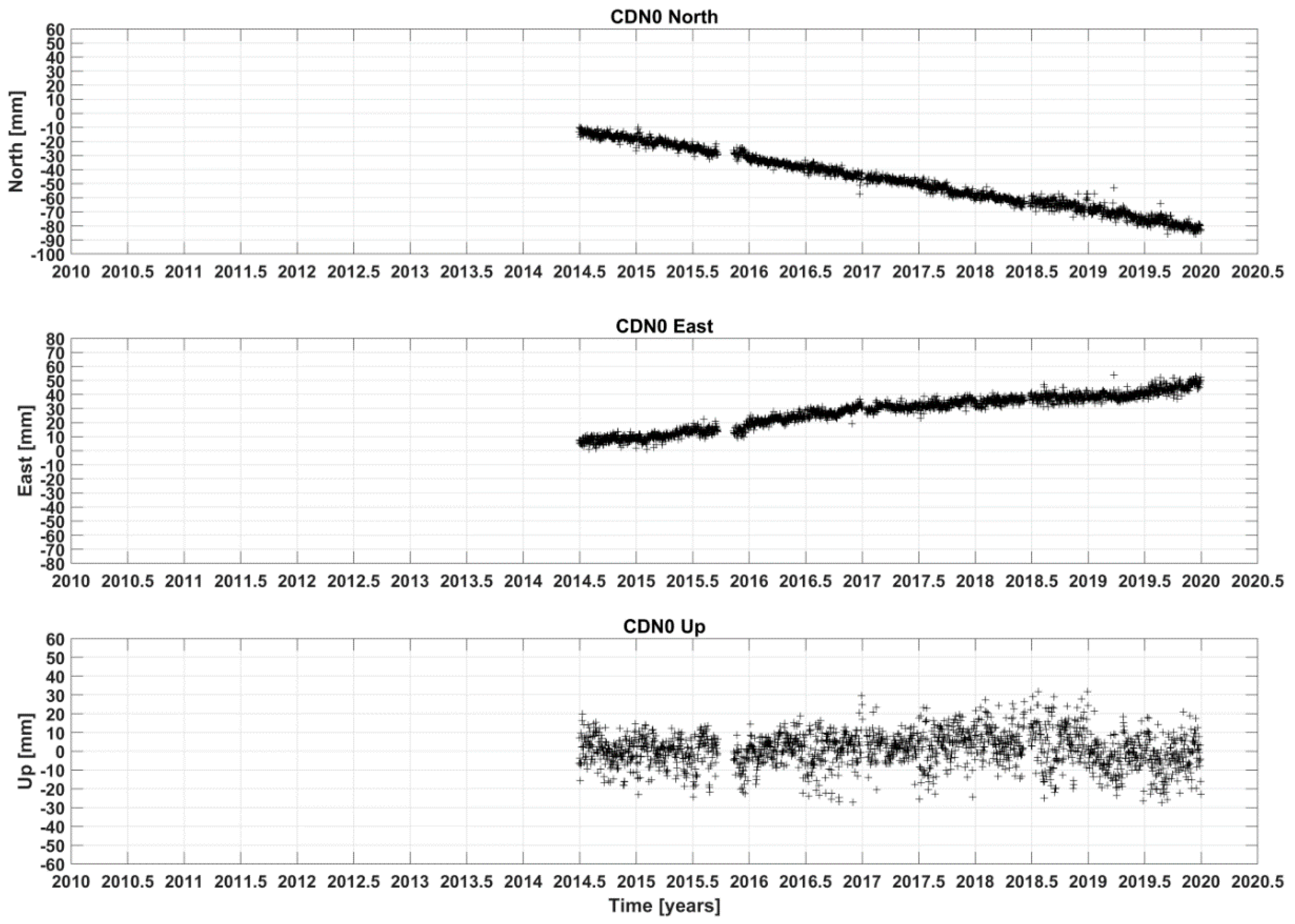
| CDN0 | N 35°20′16.02” | E 23°46′46.85” | 1049.518 | −0.0126 | 0.0075 | +0.0004 | 2014.49–2019.99 |
| CRS1 | N 35°18′12.64” | E 23°31′17.26” | 21.207 | −0.0122 | 0.0067 | −0.0007 | 2008.18–2019.99 |
| HERA | N 35°19′26.85” | E 25°08′29.41” | 90.783 | −0.0138 | 0.0072 | −0.0012 | 2010.36–2019.99 |
| IERA | N 35°03′11.04” | E 25°47′50.03” | 132.843 | −0.0143 | 0.0073 | −0.0008 | 2010.49–2019.99 |
| MEN2 | N 35°40′12.89” | E 23°44′26.30” | 265.707 | −0.0141 | 0.0060 | −0.0005 | 2013.25–2019.25 |
| MOIR | N 35°03′14.21” | E 24°52′39.90” | 135.505 | −0.0138 | 0.0072 | −0.0023 | 2012.78–2019.93 |
| PALC | N 35°14′21.77” | E 23°38′26.51” | 73.022 | −0.0120 | 0.0070 | +0.0013 | 2012.78–2019.14 |
| RDK1 | N 35°11′15.37” | E 24°19′06.53” | 25.533 | −0.0127 | 0.0079 | +0.0008 | 2009.17–2019.99 |
| RETH | N 35°23′15.92” | E 24°36′47.08” | 85.569 | −0.0134 | 0.0074 | −0.0005 | 2010.26–2019.22 |
| TUC2 | N 35°31′59.48” | E 24°04′14.01” | 160.889 | −0.0124 | 0.0071 | −0.0006 | 2004.47–2019.99 |

References
- Bojinski, S.; Verstraete, M.; Peterson, T.C.; Richter, C.; Simmons, A.; Zemp, M. The concept of essential climate variables in support of climate research, applications, and policy. Bull. Am. Meteorol. Soc. 2014, 95, 1431–1443. [Google Scholar] [CrossRef]
- Bernardo, F.; Aires, F.; Prigent, C. Atmospheric water-vapour profiling from passive microwave sounders over ocean and land Part II: Validation using existing instruments. Q. J. R. Meteorol. Soc. 2013, 139, 865–878. [Google Scholar] [CrossRef] [Green Version]
- De Rosa, B.; Di Girolamo, P.; Summa, D. Temperature and water vapour measurements in the framework of the Network for the Detection of Atmospheric Composition Change (NDACC). Atmos. Meas. Tech. 2020, 13, 405–427. [Google Scholar] [CrossRef] [Green Version]
- Devasthale, A.; Sedlar, J.; Tjerström, M. Characteristics of water-vapour inversions observed over the Arctic by Atmospheric Infrared Sounder (AIRS) and radiosondes. Atmos. Chem. Phys. 2011, 11, 9813–9823. [Google Scholar] [CrossRef] [Green Version]
- Beaton, S.P.; Spowart, M. UV absortion hygrometer for fast-response airborne water vapor measurements. J. Atmos. Ocean. Technol. 2012, 29, 1295–1303. [Google Scholar] [CrossRef]
- He, J.; Liu, Z. Comparison of satellite-derived precipitable water vapor through near-infrared remote sensing channels. IEEE Trans. Geosci. Remote Sens. 2019, 57, 10252–10262. [Google Scholar] [CrossRef]
- Hoffmann, A.; Clifford, D.; Aulinas, J.; Carton, J.C.; Deconinck, F.; Esen, B.; Hüsing, J.; Kern, K.; Kox, S.; Krejci, D.; et al. A novel satellite mission concept for upper air water vapour, aerosol and cloud observations using integrated path differential absiortion LiDAR limb sounding. Remote Sens. 2012, 4, 867–910. [Google Scholar] [CrossRef] [Green Version]
- Elliot, W.P.; Smith, M.E.; Angell, J.K. Monitoring tropospheric water vapor changes using radiosonde data. Dev. Atmos. Sci. 1991, 19, 311–327. [Google Scholar] [CrossRef]
- Han, Y.; Snider, J.B.; Westwater, E.R.; Melfi, S.H.; Ferrare, R.A. Observations of water vapor by ground-based microwave radiometers and Raman lidar. J. Geophys. Res. 1994, 99, 18695–18702. [Google Scholar] [CrossRef]
- Zhang, H.; Yuan, Y.; Li, W.; Zhang, B. A real-time precipitable water vapor monitoring system using the national GNSS network of China: Method and preliminary results. IEEE J. Sel. Top. Appl. Earth Obs. Remote Sens. 2019, 12, 1587–1598. [Google Scholar] [CrossRef]
- Donlon, C.; Berruti, B.; Buongiorno, A.; Ferreira, M.H.; Féménias, P.; Frerick, J.; Goryl, P.; Klein, U.; Laur, H.; Mavrocordatos, C.; et al. The Global Monitoring for Environment and Security (GMES) Sentinel-3 mission. Remote Sens. Environ. 2012, 120, 37–57. [Google Scholar] [CrossRef]
- Fernandes, M.J.; Lázaro, C. Independent assessment of Sentinel-3A wet tropospheric correction over the open and coastal ocean. Remote Sens. 2018, 10, 484. [Google Scholar] [CrossRef] [Green Version]
- Mertikas, S.P.; Donlon, C.; Féménias, P.; Mavrocordatos, C.; Galanakis, D.; Tripolitsiotis, A.; Frantzis, X.; Tziavos, I.N.; Vergos, G.; Guinle, T. Fifteen Years of Cal/Val Service to Reference Altimetry Missions: Calibration of Satellite Altimetry at the Permanent Facilities in Gavdos and Crete, Greece. Remote Sens. 2018, 10, 1557. [Google Scholar] [CrossRef] [Green Version]
- Mertikas, S.P.; Donlon, C.; Vuilleumier, P.; Cullen, R.; Féménias, P.; Tripolitsiotis, A. An action plan towards fiducial reference measurements for altimetry. Remote Sens. 2019, 11, 1993. [Google Scholar] [CrossRef] [Green Version]
- Mertikas, S.P.; Donlon, C.; Féménias, P.; Mavrocordatos, C.; Galanakis, D.; Tripolitsiotis, A.; Frantzis, X.; Kokolakis, C.; Tziavos, I.N.; Vergos, G.; et al. Absolute calibration of the European Sentinel-3A surface topography mission over the permanent facility for altimetry calibration in west Crete, Greece. Remote Sens. 2018, 10, 1808. [Google Scholar] [CrossRef] [Green Version]
- Bevis, M.; Businger, S.; Chiswell, S.; Herring, T.A.; Anthes, R.A.; Rocken, C.; Ware, R.H. GPS Meteorology: Mapping zenith wet delays and precipitable water. J. Appl. Meteorol. 1994, 33. [Google Scholar] [CrossRef]
- Kacmarik, M.; Dousa, J.; Dick, G.; Zus, F.; Brenot, H.; Möller, G.; Pottiaux, E.; Kaplon, J.; Hordyniec, P.; Václavovic, P.; et al. Inter-technique validation of tropospheric slant total delays. Atmos. Meas. Tech. 2017, 10, 2183–2208. [Google Scholar] [CrossRef] [Green Version]
- Vaquero-Martinez, J.; Anton, M.; de Galisteo, J.P.O.; Cachorro, V.E.; Costa, M.J.; Roman, R.; Bennouna, Y.S. Validation of MODIS integrated water vapor product against reference GPS data at the Iberian Peninsula. Int. J. Appl. Earth Obs. Geoinf. 2017, 63, 214–221. [Google Scholar] [CrossRef] [Green Version]
- Pan, L.; Guo, F. Real-time tropospheric delay retrieval with GPS, GLONASS, Galileo and BDS data. Nat. Sci. Rep. 2018, 8, 17067. [Google Scholar] [CrossRef] [Green Version]
- Mertikas, S.; Tripolitsiotis, A.; Donlon, C.; Mavrocordatos, C.; Féménias, P.; Frantzis, X.; Kokolakis, C.; Guinle, T.; Vergos, G.; Tziavos, I.N.; et al. The ESA Permanent Facility for Altimetry Calibration: Monitoring performance of Radar Altimeters for Sentinel-3A, Sentinel-3B and Jason-3 using transponder and sea-surface calibration with FRM standards. Remote Sens. 2020. under review. [Google Scholar]
- Lamquin, N.; Clerc, S.; Bourg, L.; Donlon, C. OLCI A/B Tandem Phase Analysis, Part 1: Level 1 Homogenisation and Harmonisation. Remote Sens. 2020, 12, 1804. [Google Scholar] [CrossRef]
- Sentinel-3 CalVal Team. Technical Note: Sentinel-3 OLCI-B Spectral Response Functions from Pre-Flight Characterization; S3-TN-ESA-OL-660; European Space Research and Technology Centre, European Space Agency: Noordwijk, The Netherlands, 2016. [Google Scholar]
- Schläpfer, D.; Borel, C.C.; Keller, J.; Itten, K.I. Atmospheric pre-corrected differential absorption technique to retrieve columnar water vapor. Remote Sens. Environ. 1998, 65, 353–366. [Google Scholar] [CrossRef]
- Leinweber, R. Remote Sensing of Atmospheric Water Vapor over Land Areas Using MERIS Measurements and Application to Numerical Weather Prediction Model Validation. Ph.D. Thesis, Freien Universität Berlin, Berlin, Germany, 22 June 2010. [Google Scholar]
- Fischer, J. Retrieval of Total Water Vapour Content from OLCI Measurements. ATBD Water Vapour. Available online: https://earth.esa.int/documents/247904/349589/OLCI_L2_ATBD_Water_Vapour.pdf (accessed on 20 May 2020).
- Ning, T.; Wang, J.; Elgered, G.; Dick, G.; Wickert, J.; Bradke, M.; Sommer, M.; Querel, R.; Smale, D. The uncertainty of the atmospheric integrated water vapour estimated from GNSS observations. Atm. Meas. Tech. 2016, 9, 79–92. [Google Scholar] [CrossRef] [Green Version]
- Baldysz, Z.; Nykiel, G.; Figurski, M.; Araszkiewicz, A. Assessment of the impact of GNSS processing strategies on the long-term parameters of 20 years of IWV time series. Remote Sens. 2018, 10, 496. [Google Scholar] [CrossRef] [Green Version]
- Shangguan, M.; Heise, S.; Bender, M.; Dick, G.; Ramarschi, M.; Wickert, J. Validation of GPS atmospheric water vapor with WVR data in satellite tracking mode. Ann. Geophys. 2015, 33, 55–61. [Google Scholar] [CrossRef] [Green Version]
- Tserolas, V.; Mertikas, S.P.; Frantzis, X. The western Crete geodetic infrastructure: Long-range power-law correlations in GPS time series using Detrended Fluctuation Analysis. Adv. Space Res. 2013, 51, 1448–1467. [Google Scholar] [CrossRef]
- Herring, T.A.; King, R.W.; McClusky, S.C. GAMIT Reference Manual: GPS Analysis at MIT, Release 10.7; Massachusetts Institute of Technology: Cambridge, MA, USA, 2018; Available online: http://geoweb.mit.edu/gg/GAMIT_Ref,pdf (accessed on 10 September 2018).
- Altamimi, Z.; Rebischung, P.; Métivier, L.; Collilieux, X. ITRF2014: A new release of the International Terrestrial Reference Frame modeling nonlinear station motions. J. Geophys. Res. Solid Earth 2016, 121, 6109–6131. [Google Scholar] [CrossRef] [Green Version]
- Dong, D.; Fang, P.; Bock, Y.; Cheng, M.K.; Miyazaki, S. Anatomy of apparent seasonal variations from GPS-derived site position time series. J. Geophys. Res. Sold Earth 2002, 37. [Google Scholar] [CrossRef] [Green Version]
- IERS Conventions. 36 Frankfurt am Main: Verlag des Bundesamts für Kartographie und Geodäsie; Petit, G., Luzum, B., Eds.; IERS Technical Note; IERS: Frankfurt am Main, Germany, 2010; p. 179. ISBN 3-89888-989-6. Available online: https://www.iers.org/IERS/EN/Publications/TechnicalNotes/tn36.html (accessed on 11 September 2018).
- Lyard, F.; Lefevre, F.; Letellier, T.; Francis, O. Modelling the global ocean tides: Modern insights from FES2004. Ocean Dyn. 2006, 56, 394–415. [Google Scholar] [CrossRef]
- Saastamoinen, J. Contribution to the theory of atmospheric refraction. Bull. Geod. 1975, 105, 279–298. [Google Scholar] [CrossRef]
- Tregoning, P.; van Dam, T. Atmospheric pressure loading corrections applied to GPS data at the observation level. Geophys. Res. Lett. 2005, 32, L22310. [Google Scholar] [CrossRef] [Green Version]
- Boehm, J.; Werl, B.; Schuh, H. Troposphere mapping functions for GPS and very long baseline interferometry from European Centre for Medium-Range Weather Forecasts operational analysis data. J. Geophys. Res. 2006, 111, B02406. [Google Scholar] [CrossRef]
- Henken, C.C.; Dirks, L.; Steinke, S.; Diedrich, H.; August, T.; Crewell, S. Assessment of sampling effects on various satellite-derived integrated water vapor datasets using GPS measurements in Germany as reference. Remote Sens. 2020, 12, 1170. [Google Scholar] [CrossRef] [Green Version]
- Lindenbergh, R.; Keshin, M.; van der Marel, H.; Hansen, R. High resolution spatiotemporal water vapour mapping using GPS and MERIS observations. Int. J. Remote Sens. 2008, 29, 2393–2409. [Google Scholar] [CrossRef]
- Sentinel-3 Data Product Quality Reports. Available online: https://sentinels.copernicus.eu/documents/247904/4069162/Sentinel-3-MPC-ACR-OLCI-Cyclic-Report-056-037.pdf (accessed on 19 May 2020).
- Makarau, A.; Richter, R.; Schläpfer, D.; Reinartz, P. APDA Water Vapor Retrieval Validation for Sentinel-2 Imagery. IEEE Geosci. Remote Sens. Lett. 2017, 14, 227–231. [Google Scholar] [CrossRef] [Green Version]


| File | Cycle | Relative Orbit | Sensing Date, Time | Image X | Image Y | IWV [kg/m2] | IWV_Average [kg/m2] | IWV Error |
|---|---|---|---|---|---|---|---|---|
| Name 1 | 4 | 7 | 6/5/2016, 8:44 | 2030 | 3157 | – | 15.75 | – |
| Name | 4 | 7 | 6/5/2016, 8:44 | 2060 | 3077 | 20.70 | 19.55 | 0.90 |
| Orbit No. | Sentinel-3A | Sentinel-3B | ||
|---|---|---|---|---|
| Cycle No. | Defective Cycle [Left out] | Cycle No. | Defective Cycle [Left out] | |
| 7 | 4-55 | 17 | 21-34 | 25, 26, 27, 28 |
| 21 | 4-55 | 21 | 21-34 | 24 |
| 64 | 4-55 | - | 21-33 | 23, 24, 25 |
| 78 | 4-55 | 12, 14, 16, 23 | 24-33 | 27 |
| 121 | 4-55 | 30, 38, 41 | 21-33 | 24, 31 |
| 135 | 4-55 | 4, 12, 37 | 22-33 | 24 |
| 178 | 4-55 | 10, 43 | 22-33 | 23, 24 |
| 235 | 4-55 | 38 | 23-33 | - |
| 278 | 4-55 | - | 21-33 | 24, 25 |
| 292 | 3-55 | 12 | 20-33 | 25 |
| 335 | 3-55 | 27 | 21-33 | - |
| 349 | 3-55 | 14 | 21-33 | 24, 25, 26, 27 |
| Site | IWVsgl | IWVavg. | IWVGNSS | Diff. OLCI(sgl)-GNSS | Diff. OLCI(avg)-GNSS | |||||
|---|---|---|---|---|---|---|---|---|---|---|
| Mean | SD | Mean | SD | Mean | SD | Mean | SD | Mean | SD | |
| CDN0 | +12.27 | ±5.25 | +15.47 | ±5.93 | +13.22 | ±5.10 | −1.09 | ±2.43 | +2.31 | ±2.63 |
| CRS1 | +22.50 | ±6.86 | +20.58 | ±6.51 | +21.20 | ±6.29 | +1.38 | ±2.70 | −0.56 | ±1.96 |
| HERA | +23.06 | ±7.66 | +21.96 | ±7.42 | +21.07 | ±6.87 | +1.94 | +1.98 | +0.89 | ±1.55 |
| IERA | +21.02 | ±7.33 | +18.80 | ±6.85 | +19.62 | ±6.62 | +1.23 | ±2.33 | −0.82 | ±1.79 |
| MEN2 | +19.33 | ±6.30 | +18.52 | ±6.34 | +19.63 | ±6.34 | −0.56 | ±1.69 | −1.11 | ±1.60 |
| MOIR | +20.72 | ±7.38 | +20.46 | ±7.14 | +19.92 | ±6.72 | +0.91 | ±2.01 | +0.55 | ±1.62 |
| PALC | +21.65 | ±6.92 | +19.13 | ±6.39 | +20.54 | ±6.39 | +1.03 | +2.31 | −1.40 | ±1.63 |
| RDK1 | - | - | +17.46 | ±6.53 | +21.50 | ±6.55 | - | - | −4.05 | ±2.69 |
| RETH | +21.98 | ±7.20 | +21.77 | ±7.17 | +20.75 | ±6.81 | +1.09 | ±2.14 | +1.02 | ±1.59 |
| TUC2 | +20.65 | ±7.16 | +21.30 | ±7.19 | +20.36 | ±6.49 | +0.31 | ±2.10 | +0.94 | ±1.85 |
| Mean | +20.35 mm | +19.55 mm | +19.78 mm | |||||||
| SD | ±3.23 mm | ±2.07 mm | ±2.39 mm | |||||||
| Site | Offset [mm] | Slope | R2 | Pearson Coefficient | ||||
|---|---|---|---|---|---|---|---|---|
| Single | Average | Single | Average | Single | Average | Single | Average | |
| CDN0 | −0.26 | +1.71 | 0.93 | 1.04 | 0.80 | 0.81 | 0.89 | 0.89 |
| CRS1 | 1.08 | −0.58 | 1.01 | 0.99 | 0.86 | 0.93 | 0.93 | 0.96 |
| HERA | 0.11 | −0.31 | 1.09 | 1.06 | 0.94 | 0.96 | 0.97 | 0.98 |
| IERA | 0.24 | −0.79 | 1.05 | 0.99 | 0.90 | 0.93 | 0.95 | 0.96 |
| MEN2 | 0.47 | −0.33 | 0.95 | 0.96 | 0.93 | 0.94 | 0.96 | 0.97 |
| MOIR | −0.23 | −0.14 | 1.06 | 1.03 | 0.93 | 0.95 | 0.96 | 0.97 |
| PALC | 0.73 | −0.74 | 1.02 | 0.97 | 0.89 | 0.94 | 0.94 | 0.98 |
| RDK1 | - | −2.16 | - | 0.91 | - | 0.84 | - | 0.92 |
| RETH | 1.02 | 0.48 | 1.00 | 1.03 | 0.91 | 0.95 | 0.96 | 0.98 |
| TUC2 | −0.63 | −0.54 | 1.05 | 1.07 | 0.92 | 0.94 | 0.96 | 0.97 |
| Site | IWVsgl | IWVavg. | IWVGNSS | Diff. OLCI(sgl)-GNSS | Diff. OLCI(avg)-GNSS | |||||
|---|---|---|---|---|---|---|---|---|---|---|
| Mean | SD | Mean | SD | Mean | SD | Mean | SD | Mean | SD | |
| CDN0 | +12.20 | ±5.44 | +15.18 | ±5.95 | +11.90 | ±4.91 | −0.30 | ±1.64 | −3.46 | ±2.05 |
| CRS1 | +22.34 | ±7.06 | +20.01 | ±6.06 | +20.43 | ±6.04 | −1.90 | ±2.56 | +0.23 | ±1.63 |
| HERA | +22.71 | ±7.51 | +21.31 | ±6.93 | +20.34 | ±6.73 | −2.37 | ±2.20 | −1.07 | ±1.69 |
| IERA | +21.28 | ±7.77 | +19.05 | ±7.03 | +19.60 | ±6.80 | +1.68 | ±3.13 | +0.71 | ±1.76 |
| MEN2 | not estimated due to insufficient sample | |||||||||
| MOIR | +20.79 | ±7.43 | +20.72 | ±7.16 | +19.72 | ±6.85 | −1.07 | ±1.89 | −0.74 | ±1.60 |
| PALC | not estimated due to insufficient sample | |||||||||
| RDK1 | - | - | +16.26 | ±6.13 | +20.52 | ±6.85 | - | - | +4.27 | ±3.13 |
| RETH | +21.40 | ±6.84 | +21.26 | ±6.89 | +20.65 | ±6.74 | −0.75 | ±1.83 | −0.65 | ±1.72 |
| TUC2 | +19.89 | ±6.72 | +20.29 | ±6.81 | +18,92 | ±6.52 | −0.97 | ±1.77 | −1.57 | ±1.53 |
| Mean | +20.09 mm | +19.26 mm | +19.02 mm | |||||||
| SD | ±3.60 mm | ±2.32 mm | ±3.17 mm | |||||||
| Site | Offset [mm] | Slope | R2 | Pearson Coefficient | ||||
|---|---|---|---|---|---|---|---|---|
| Single | Average | Single | Average | Single | Average | Single | Average | |
| CDN0 | −0.41 | 1.78 | 1.06 | 1.14 | 0.91 | 0.90 | 0.96 | 0.95 |
| CRS1 | 0.02 | 0.70 | 1.09 | 0.95 | 0.87 | 0.93 | 0.94 | 0.96 |
| HERA | 0.96 | 1.42 | 1.07 | 0.98 | 0.92 | 0.94 | 0.96 | 0.97 |
| IERA | 0.75 | −0.25 | 1.05 | 0.98 | 0.84 | 0.94 | 0.91 | 0.97 |
| MEN2 | not estimated due to insufficient sample | |||||||
| MOIR | 0.07 | 0.35 | 1.05 | 1.02 | 0.94 | 0.95 | 0.97 | 0.97 |
| PALC | not estimated due to insufficient sample | |||||||
| RDK1 | - | −0.09 | - | 0.78 | - | 0.79 | - | 0.89 |
| RETH | 1.19 | 1.21 | 0.98 | 0.97 | 0.93 | 0.94 | 0.96 | 0.97 |
| TUC2 | 1.09 | 1.16 | 0.99 | 1.02 | 0.93 | 0.95 | 0.96 | 0.97 |
| Site | Sentinel-3A OLCI(A) | Sentinel-3B OLCI(B) |
|---|---|---|
| Crete | −0.23 mm | +0.24 mm |
| S3MPC | +1.24 mm | +1.02 mm |
| Δ[Crete-S3MPC] | 1.47 mm | 0.78 mm |
© 2020 by the authors. Licensee MDPI, Basel, Switzerland. This article is an open access article distributed under the terms and conditions of the Creative Commons Attribution (CC BY) license (http://creativecommons.org/licenses/by/4.0/).
Share and Cite
Mertikas, S.; Partsinevelos, P.; Tripolitsiotis, A.; Kokolakis, C.; Petrakis, G.; Frantzis, X. Validation of Sentinel-3 OLCI Integrated Water Vapor Products Using Regional GNSS Measurements in Crete, Greece. Remote Sens. 2020, 12, 2606. https://0-doi-org.brum.beds.ac.uk/10.3390/rs12162606
Mertikas S, Partsinevelos P, Tripolitsiotis A, Kokolakis C, Petrakis G, Frantzis X. Validation of Sentinel-3 OLCI Integrated Water Vapor Products Using Regional GNSS Measurements in Crete, Greece. Remote Sensing. 2020; 12(16):2606. https://0-doi-org.brum.beds.ac.uk/10.3390/rs12162606
Chicago/Turabian StyleMertikas, Stelios, Panagiotis Partsinevelos, Achilleas Tripolitsiotis, Costas Kokolakis, George Petrakis, and Xenophon Frantzis. 2020. "Validation of Sentinel-3 OLCI Integrated Water Vapor Products Using Regional GNSS Measurements in Crete, Greece" Remote Sensing 12, no. 16: 2606. https://0-doi-org.brum.beds.ac.uk/10.3390/rs12162606