On the Radiative Transfer Model for Soil Moisture across Space, Time and Hydro-Climates


1
Department of Biological and Agricultural Engineering, Texas A&M University, College Station, TX 77843, USA
2
NASA Goddard Space Flight Center, Greenbelt, MD 20771, USA
3
Science Systems and Applications, Lanham, MD 20706, USA
*
Author to whom correspondence should be addressed.
Remote Sens. 2020, 12(16), 2645; https://0-doi-org.brum.beds.ac.uk/10.3390/rs12162645
Submission received: 15 June 2020
/
Revised: 24 July 2020
/
Accepted: 24 July 2020
/
Published: 17 August 2020
(This article belongs to the Special Issue Remote Sensing and Modeling of the Terrestrial Water Cycle)
Abstract
:A framework is proposed for understanding the efficacy of the microwave radiative transfer model (RTM) of soil moisture with different support scales, seasonality (time), hydroclimates, and aggregation (scaling) methods. In this paper, the sensitivity of brightness temperature TB (H- and V-polarization) to physical variables (soil moisture, soil texture, surface roughness, surface temperature, and vegetation characteristics) is studied. Our results indicate that the sensitivity of brightness temperature (V- or H-polarization) is determined by the upscaling method and heterogeneity observed in the physical variables. Under higher heterogeneity, the TB sensitivity to vegetation and roughness followed a logarithmic function with an increasing support scale, while an exponential function is followed under lower heterogeneity. Surface temperature always followed an exponential function under all conditions. The sensitivity of TB at H- or V- polarization to soil and vegetation characteristics varied with the spatial scale (extent and support) and the amount of biomass observed. Thus, choosing an H- or V-polarization algorithm for soil moisture retrieval is a tradeoff between support scales, and land surface heterogeneity. For largely undisturbed natural environments such as SGP’97 and SMEX04, the sensitivity of TB to variables remains nearly uniform and is not influenced by extent, support scales, or an upscaling method. On the contrary, for anthropogenically-manipulated environments such as SMEX02 and SMAPVEX12, the sensitivity to variables is highly influenced by the distribution of land surface heterogeneity and upscaling methods.
1. Introduction
The remote sensing community aims to develop soil moisture products at various resolutions, as soil moisture finds application from local (e.g., crop water management) and regional (e.g., flood and drought forecasting) to global scales (e.g., meteorology, climate dynamics) [1]. The active or passive sensors used for estimating soil moisture come with their own challenges such as accuracy, Radio Frequency Interference (RFI), high sensitivity to vegetation/roughness, spatio-temporal coverage, big data challenges, etc., [2,3]. Developing fine resolution soil moisture products can be achieved either by downscaling retrieved coarse-resolution soil moisture or downscaling the observed brightness temperature (TB) followed by soil moisture retrieval [4,5,6,7]. Several scaling algorithms have been developed in the past using data fusion techniques integrating information from various scales (point/airborne/satellite), platforms (MODIS/LANDSAT/AVHRR etc.), sensors (active/passive), frequencies (P, L, C, and X), and land surface variables (surface temperature, NDVI, etc.) [8,9,10,11,12]. For most cases, coarse-scale knowledge is estimated from smaller spatial scale features in which upscaling has reduced to the problem of a change of support scale. Western and Bloschl (1999) [13] defined the scale triplet (support, spacing, and extent), where support is referred to the area (or volume) integrated by individual soil moisture measurements. The scaling methods incorporate their own conceptual model uncertainties apart from the uncertainties of products used for downscaling/upscaling [14,15,16]. Thus, for downscaling/upscaling of either soil moisture or TB, it first calls for understanding the propagation of errors/uncertainties through the scale and heterogeneity of land surface variables.
The two main issues that still undermine the large scale monitoring of soil moisture are scaling and land surface heterogeneity [17,18,19]. Scaling of microwave theory/models developed over small spatial scales to coarser spatial scales has been a subject of research for the past three decades. Most environmental processes are non-linear in nature and the land surface variables (and their interactions) responsible for these processes vary across scales (space and time) [20,21,22] resulting in complex scaling relationships. The sub-footprint landscape heterogeneity compromises the satellite-based soil moisture retrieval accuracy [23,24,25]. For example, within a hydroclimate, the heterogeneity in land surface variables observed at 30 m resolution will be different from 100 m, 1 km, 5 km, and so on, and will be different if observed at different time periods, frequencies, polarizations, etc. There can also be considerable effects on retrieved soil moisture if the extent of the analysis or footprint shape/size varies, changing the range of heterogeneity observed for land surface variables. Thus, model calibration of soil-vegetation parameters across land surface heterogeneity and scale pose a challenge for remote sensing retrieval of soil moisture.
The analysis in this paper is a follow-up to Neelam and Mohanty, (2015) [26], where the global sensitivity analysis was initially used to evaluate the microwave RTM at a field scale for the first and second order sensitivities to land surface variables along with non-linear interactions between them. In this paper, we advance our current knowledge about the microwave RTM under varying heterogeneity in land surface variables (soil moisture, soil texture, surface roughness, surface temperature, and vegetation characteristics, i.e., vegetation water content, vegetation structure, and scattering albedo) through support scales, time and hydro-climates, and in the presence of land surface interactions. Here, the attention is also drawn towards the appropriate representation (upscaling) of the spatial heterogeneity and its influence brightness temperature at multiple scales. Our overarching goal here is to propose a framework for understanding the efficacy of the microwave radiative transfer model (RTM) for soil moisture retrieval with different support scales, seasonality (time), and under land surface heterogeneity. We performed the analysis using two-dimensional spatial maps of land surface variables as model inputs beginning from an airborne 800 m and 1.5 km support scale. These variables are then upscaled to various supports (1.6 km, 3.2 km, 6.4 km, and 12.8 km), using two different averaging methodologies, to study the influence of upscaling methods on an RTM performance. Adopting the global spatial sensitivity analysis (GSSA) [27,28,29,30], the sensitivity to soil and vegetation characteristics across scales are evaluated.
2. Materials and Method
2.1. Heterogeneity Observed in Various Hydroclimates
The effects of varying heterogeneity on brightness temperature are studied in four different hydroclimates using data from field campaigns, namely SGP97 (Southern Great Plains’1997), SMEX02 (Soil Moisture Experiment’2002), SMEX04 (Soil Moisture Experiment’2004), and SMAPVEX12 (Soil Moisture Active Passive Experiment’2012). These field campaigns were conducted over approximately a 4–8 weeks’ window, primarily to validate soil moisture retrieval algorithms over a wide range of soil and vegetation conditions [31,32,33]. The airborne remote sensing data for these field campaigns were observed at either 800 m or 1.5 km resolution, which is the base resolution for our analysis. The 800 m pixels are upscaled to support scales of 1.6 km, 3.2 km, 6.4 km, and 12.8 km, and 1.5 km pixels are upscaled to 3 km and 9 km to coincide with two of the Soil Moisture Active Passive (SMAP) target products. The variables such as soil moisture, surface temperature, vegetation water content, and soil texture are obtained from various sources, which are discussed under each field campaign. Variables such as surface roughness, vegetation structure, and single scattering albedo, which are available only at sparse locations, are assumed to be scalars with a uniform probability distribution whose ranges are estimated from extensive field measurements.
2.1.1. Southern Great Plains Experiment’1997 (SGP’97), Oklahoma
The SGP’97 hydrology experiment was conducted in the sub-humid (Köppen climate classification-Cfa) [34] region of central Oklahoma from 18 June through 17 July 1997. The topography of the region is moderately rolling and soils vary with a wide range of textures, including large regions of both coarse and fine textures, and with an average annual rainfall and temperature of 750 mm and 288.85 K, respectively. The land use is dominated by rangeland and pasture with significant areas of winter wheat and other crops. The L-band Electronically Scanned Thinned Array Radiometer (ESTAR) was used to measure soil moisture at 800 m × 800 m resolution. An 800 m resolution daily effective soil temperature maps were generated using the ground-based soil temperatures and grid-based resampling program. The vegetation water content (VWC) map at 800 m resolution was developed from normalized difference vegetation index (NDVI) values computed using the Landsat TM imagery collected on 25 July 1997 [35]. A combination of soil geographic database (STATSGO) and soil texture samples were used to develop a resampled texture map at 800 m resolution [23].
2.1.2. Soil Moisture Experiment’2002 (SMEX02), Iowa
The SMEX02 experiment was conducted in Walnut Creek watershed, Iowa, from 23 June through 12 July 2002. This region is classified as a humid climate (Köppen climate classification-Dfa) with an average annual rainfall of 835 mm and a temperature of 283 K. A considerable amount of variability in soil texture is observed in the region, ranging from fine sandy loam to clay with the majority classified as silt loam with relatively low permeability [36]. Corn and soybean crops are the two dominant land covers of Iowa, covering approximately 50% and 40%, respectively. The C-band Polarimeteric Scanning Radiometer (PSR-C) retrieved soil moisture at 800 m × 800 m resolutions [37] and was used for the analysis. A total of four days (DOY 178, 182, 186, and 188) were selected to capture the temporal variability in land surface heterogeneity due to crop growth, temperature, and soil moisture changes. The Soil Survey Geographic Database (SSURGO) and Landsat-7/5 E/TM derived vegetation water content at 30 m that was resampled to 800 m × 800 m grids. The averages of the surface and 1-cm depth soil temperature were interpolated through kriging to obtain coverage for a grid size of 800 m.
2.1.3. Soil Moisture Experiment’2004 (SMEX04), Arizona
The SMEX04 field campaign was conducted with a primary focus on Walnut Gulch (WC) Experimental Watershed near Tombstone, which is operated by the Agriculture Research Service (ARS), U.S. Department of Agriculture (USDA), between 2 August and 27 August 2004 [31]. The climate of this region is classified as semi-arid (Köppen climate classification-BSh), with a mean annual temperature of 290.85 K and receiving an average annual precipitation of 350 mm. The soils are generally well drained calcareous and gravelly loam with large percentages of rock ranging from nearly 0% on shallow slopes to over 70% on the very steep slopes. Vegetation of this region is mainly comprised of two-thirds of shrubs and the remaining one-third is grassland. The polarimetric scanning radiometer (PSR) C-band retrieved soil moisture and regularly spaced grid of 800 m resolution was used. The ground-based temperatures (surface and 5 cm temperatures are averaged) and MODIS (MOD11A1) surface temperature product are interpolated (kriging) to generate an 800 m resolution surface temperature map. The 800 m resolution vegetation water content map was developed by interpolating high resolution Landsat TM and regularly ground sampled VWC [38]. The SSURGO data at 30 m were resampled to obtain a soil texture map at 800 m resolution. A total of four days (DOY 221, 222, 225, and 226) were selected based on the availability of datasets to study the temporal variability in land surface heterogeneity. The surface roughness data were collected extensively over the Walnut Gulch (WG) watershed and sparely over the entire SMEX04 region using a pin board.
2.1.4. Soil Moisture Active Passive Validation Experiment’2012 (SMAPVEX12), Winnipeg
SMAPVEX12 was conducted from 6 June to 17 July 2012, in Winnipeg, Manitoba (Canada), which is classified as having extreme humid climate (Köppen climate classification-Dfb), with average an annual precipitation and temperature of 521 mm and 289 K, respectively. The region captures a wide variety of variability in land cover and soil texture within a few kilometers while moving from southeast to northwest [33]. The agricultural crops (mainly cereals, soybeans, canola, and corn) dominate the southeast with heavy clay soils, whereas the north and east see more lighter sandy and loamy soils with mixed land cover including forest and perennial pastures along with a few crop fields. The analysis was conducted for all days (DOY 164, 167, 169, 174, 177, 179, 181, 185, 187, 192, 195, 196, and 199) using the Passive Active L-band System (PALS) derived soil moisture and surface temperature at 1.5 km resolution [39]. The VWC available at 5 m resolution estimated from the Normalized Difference Water Index (NDWI) using SPOT and RapidEye satellite overpasses was resampled to 1.5 km grids.
2.2. Soil Moisture Retrieval Algorithm
The approach followed in this study was based on forward modeling using a first-order microwave radiative transfer model (RTM), also called a tau-omega (τ-ω) model [40], which is described in Equation (1) to simulate brightness temperature (,
where is the brightness temperature [K]; is the effective surface temperature [K]; Tc is the effective vegetation temperature [K]; is the emissivity of the (rough) soil surface; is the rough surface reflectivity; is the nadir optical depth; is the single scattering albedo. The subscripts p, θ, and f denote the polarization, angle of incidence, and frequency of measurement, respectively. It is assumed that the canopy and soil temperature are equal during morning thermal crossover, which also corresponds to the planned time of observation for SMAP at around 6:00 h local sun time.
The microwave signal incident emitted from the soil-vegetation layer is modified, scattered, and attenuated due to the physical and structural properties of this medium. The radiative transfer (Equation (1)) is a first-order approximation and summation of three components: (i) the direct emission by soil and one-way attenuation by canopy (the first term), (ii) direct upward emission by canopies (the second term), and (iii) emission by plants and reflected by soil and thereafter attenuated by vegetation (the third term). The physical attributes of soil layer that influence the microwave emissions are surface reflectivity and effective soil temperature , as given in Equation (1). The physical attributes of the vegetation that influence the microwave emissions are: the optical thickness of the vegetation , and the single scattering albedo . The formulation in Equation (1) is based on the assumptions that, (i) the diffuse scattering is ignored; (ii) the air-vegetation reflectivity is assumed zero, thus ignoring losses at the boundary; and (iii) the refractive index of the vegetation is approximately equal to air, which allows us to use the air-soil reflectivity in Equation (1). The extinction optical thickness of the vegetation is estimated as a product of vegetation water content (VWC) and the structure of the canopy (b). Due to the complex geometry of the natural canopies, approximate values are used for the canopy structure (b). The vegetation water content is estimated using the Normalized Difference Vegetation Index (NDVI) and regression equation [41]. The and are polarization dependent because there are differences in propagation of H-polarized and V-polarized waves under different canopy structures [42,43,44,45]. The surface roughness represents the small-scale surface undulations. These surface undulations are typically measured using a pin-board or a grid board, where the variation in elevations of metal pins are considered due to the rough surface underneath. However, due to the infeasibility of doing these measurements operationally at airborne footprints (1.5 km, 3 km, etc.). Neelam et al., 2020 [46], developed a multi-scale surface roughness model based on variables such as soil moisture, leaf area index (LAI), clay fraction (CF), and topographic curvature. Nonetheless, the current SMAP operational algorithm uses static surface roughness parameters based on IGBP land cover classes [47].
2.3. Global Spatial Sensitivity Analysis: Sobol Method
The Global Spatial Sensitivity Analysis (GSSA) [27,30] relies on Sobol methods [48], which can deal with non-linear and non-monotonic relationships between inputs and output [49,50,51,52]. These methods are based on the functional decomposition of variance (ANOVA) of the model prediction (Y) into partial variances caused due to each model input (X) (either considered singularly or in combination), i.e.,
where is the share of the output variance explained by the ith model input, is the share of the output variance explained by the interaction of the ith and jth inputs, and k is the total number of inputs. The partial variances are explained as , and so on for higher order interactions, where E and V are the expectation and variance operators; refer to the Appendix A for more details. The so-called “Sobol” indices or “variance-based sensitivity indices” are obtained as follows:
First Order Sensitivity Index the amount of variance of Y explained by input variable Xi; Second Order Sensitivity Index the amount of variance of Y explained by the interaction of the factors Xi and Xj (i.e., sensitivity to Xi and Xj not expressed in Vi nor Vj); Total Sensitivity Index , which accounts for all the contributions to the output variation due to factor Xi (i.e., the first-order index plus all its interactions). In other words, the index is defined as a summation of the main, second, and higher order effects, which involves the evaluation over a full range of parameter space. If and are equal and the sum of (and thus is 1, then the model is additive (linear) in nature, otherwise if is greater than and ∑ Si < 1 or ∑ STi > 1, then the model exhibits non-linearity. Thus, linearity or non-linearity of model through time, scale, and hydroclimate can be determined from a summation of s indices.
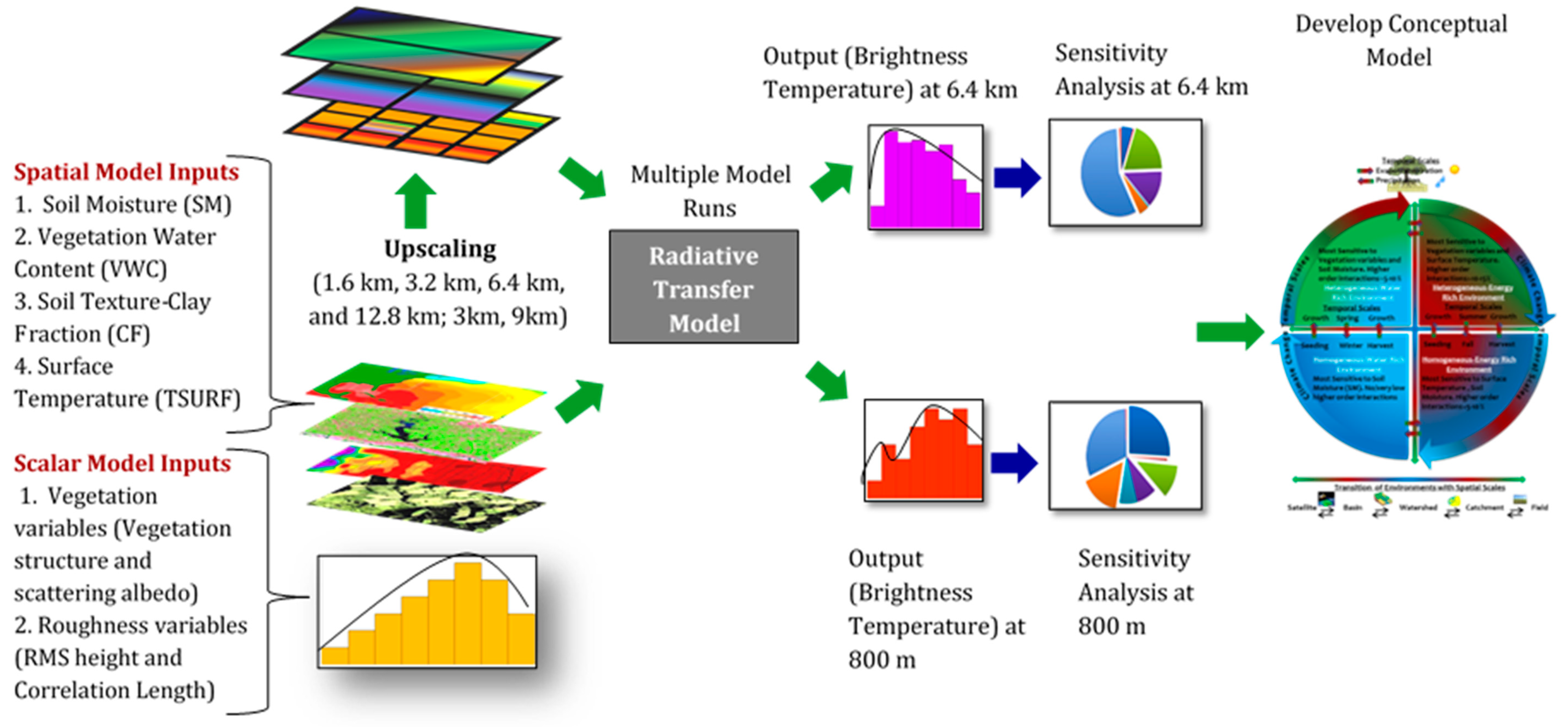
Let Y = f(X) be a spatial model, then Y is the model output and X are random independent model inputs, where X is composed of U and W, with U defined as random vectors and W defined as two-dimensional spatial maps. Using the similar configuration, Y is the simulated brightness temperature, f is the radiative transfer model, and XK is the input parameter vector with K = [X1, X2, X3, X4] as [Surface Roughness-RMS height (S), Surface Roughness-Correlation length (L), Vegetation Structure (B), Scattering Albedo (ω)] and W as spatial maps [Soil Moisture (SM), Clay Fraction (CF), Surface Temperature (TSURF), Vegetation Water Content (VWC)]. The steps used to carry out the analysis are described in Figure 1. The variables such as RMS height (S) and correlation length (L) are sampled from a uniform distribution whose ranges are estimated from field measurements. The variables such as vegetation structure (B) and scattering albedo (ω) are also sampled from a uniform distribution whose ranges are defined based on vegetation type. However, experimental data for these variables are limited and are obtained from past literature [42,53]. The range of variability in surface roughness, vegetation parameter, and scattering albedo are assumed to remain constant at all scales, as there are no means to ascertain how those vary with scale. The mean values of land surface variables used in the analysis for various field campaigns are represented in Table 1. The spatial input variable at each support scale is defined as a real random variable with a uniform range for the number of pixels developed at that scale. That is, the numbers of pixels ‘n’ at each support scale are considered as equiprobable, with each pixel labeled with a unique integer in the set {1, …, n}. The number of pixels decreases with increasing the support scale, for example, the numbers of pixels at a 800 m support scale are more than 4000, and at a 12.6 km support scale, there are about 50 pixels. The first order and total Sobol sensitivity indices are estimated with confidence intervals using the bootstrap technique with resampling [54]. The number of samples N = 55,000 are used for model evaluations. Here, we discuss and present only total sensitivity indices.
The current SMAP Level 2 and 3 radiometer-based soil moisture algorithm [47] uses vegetation and surface roughness parameters from the look up table by IGBP class, assuming sub footprint-scale homogeneity for vegetation and roughness parameters. However, surface roughness parameters change with soil type, vegetation conditions, wind speed, amount of precipitation, etc. Similarly, vegetation parameters vary with growing season, vegetation type, and structure. Due to the heterogeneous and dynamic nature of these land surface variables (varying with space and time), assuming them to be fixed parameters will introduce high errors into soil moisture retrievals. Since the range for vegetation and roughness variables are obtained from the respective field campaign conducted over a few weeks, larger heterogeneities of land surface variables are possible to occur in real time, as we have considered in our analysis.
2.4. Upscaling Methods: Linear Upscaling vs. Inverse Distance Weighted (IDW) Upscaling
Scaling is an important aspect, and is studied in various disciplines including hydrology [55,56] meteorology [57], ecology [58], and geography [59]. The upscaling and validation of satellite soil moisture products are discussed in Crow et al. (2012) [60], Qin et al. (2015) [61], Chen et al. (2016) [62], and Colliander et al. (2017) [63,64,65]. The upscaling technique for any remotely sensed land surface variable depends on the heterogeneity exhibited by the variable and antenna gain function, which plays a significant role in capturing the heterogeneity. In this paper, we investigate the difference in sensitivity of the retrieval model to the land surface variables when the variables are upscaled linearly and through Inverse Distance Weighted (IDW) to various support scales (0.8 km, 1.6 km, 3.2 km, 6.4 km, and 12.8 km). This is important because of three main reasons: (1) as the support scale changes (upscaling or downscaling), the heterogeneity of the landscape also varies. Thus, the processes that appear linear may become non-linear and vice versa. The variables that are important at one scale and hydroclimate may become trivial at another scale and hydroclimate. (2) The non-linearity of the radiative transfer model varies with heterogeneity observed for the retrieval scale. The non-linear retrieval model may show no scale effect when the scale of analysis (support) is homogeneous [66,67], and (3) the upscaling techniques become significant in heterogeneous landscapes to represent the non-linear effects [36,68,69,70,71]. In the case of a homogeneous environment, the scaling methods do not significantly influence the output, as is also validated in Wu and Liang Li (2009) [72]. The use of an unsuitable upscaling method or inappropriate representation of spatial distribution can lead to potentially wrong decisions. An inappropriate upscaling can have an even more profound impact if the result is used as an input for simulations, where a small error or distortion can cause models to produce false estimation.
IDW is a deterministic non-linear interpolation technique that uses the weighted upscaling of the attribute values from the nearby sample sub-grid to estimate the magnitude of the attribute at a higher support scale. The superior performance of IDW in comparison to other scaling methods is also discussed in Weber and Englund (1994) [73], Moyeed and Papritz (2002) [74], and Babak and Deutsch (2009) [75]. The weight a particular sub-grid that is assigned in the averaging scheme depends on the distance of the sub-grid from the center of the coarser grid. It is an averaging method based on the principle that a sample closer to the prediction location has more influence on the prediction than a sample farther apart. For gridded data, the IDW approach can be realized as a-3 dB function where higher weights are given to grid cells closer to the center of the pixel than grid cells further apart. This incorporates neighboring heterogeneity, which changes with the support scale. For this analysis, the weight of the point changes with the inverse square of the distance known as Inverse Distance Squared (IDS) upscaling. This technique is also used in the SMAP L1C [76] radiometer data product to average non-uniformly all the brightness temperature data samples that fall within the grid cell.
3. Results and Discussion
It is observed from Figures 3–6 that the brightness temperature at V-polarization is more sensitive to soil moisture, soil texture (clay fraction), and surface temperature than H-polarization under all conditions (space and time). On the other hand, H-polarization is always observed to be more sensitive to surface roughness variables (S and L) than V-polarization under all conditions. The SMEX02 and SMEX04 field campaigns were conducted using a Polarimetric Scanning Radiometer C-band (PSR/C), whereas SGP’97 and SMAPVEX12 were conducted using a Passive Active L-band System (PALS) radiometer, as mentioned earlier. Though the temporal analysis has been conducted for each hydro-climate, for the sake of brevity, we presented results for one DOY and discuss the general temporal trends observed. Neelam and Mohanty, 2015, present a detailed analysis and discussion for temporal variability in RTM sensitivity analysis. In the following sections, we discuss the variability observed in the sensitivity of the L-band brightness temperature at V- and H-polarization under: (1) Plant Structure, (2) Spatio-Temporal Scales, and (3) Upscaling and Environmental Heterogeneity.
3.1. Plant Structure
It is well understood that vegetation attenuates the microwave emission from the soil, and adds its own radiative flux to the total emission. The extent of attenuation depends on the amount of vegetation and its structure. A crop canopy may be divided into three main components: (1) leaves, (2) stalks, and (3) heads. The attenuation of radiation may, thus, occur at two layers, the upper layer consisting of heads, and a lower layer composed of leaves and stalks. The propagation characteristics are different for different canopies depending on the emission and scattering properties of these layers. Therefore, assuming polarization-independence may not be true especially for plants where the vegetation biomass is concentrated in vertically oriented dipole-like stalks and row crops. For the zero order radiative transfer model (tau-omega model), the effects of vegetation are represented by vegetation water content (VWC), single scattering albedo (ω), and vegetation structure parameter (B), where VWC captures the amount of water content in biomass, ‘B’ represents the canopy architecture, and ω represents scattering within the canopy.
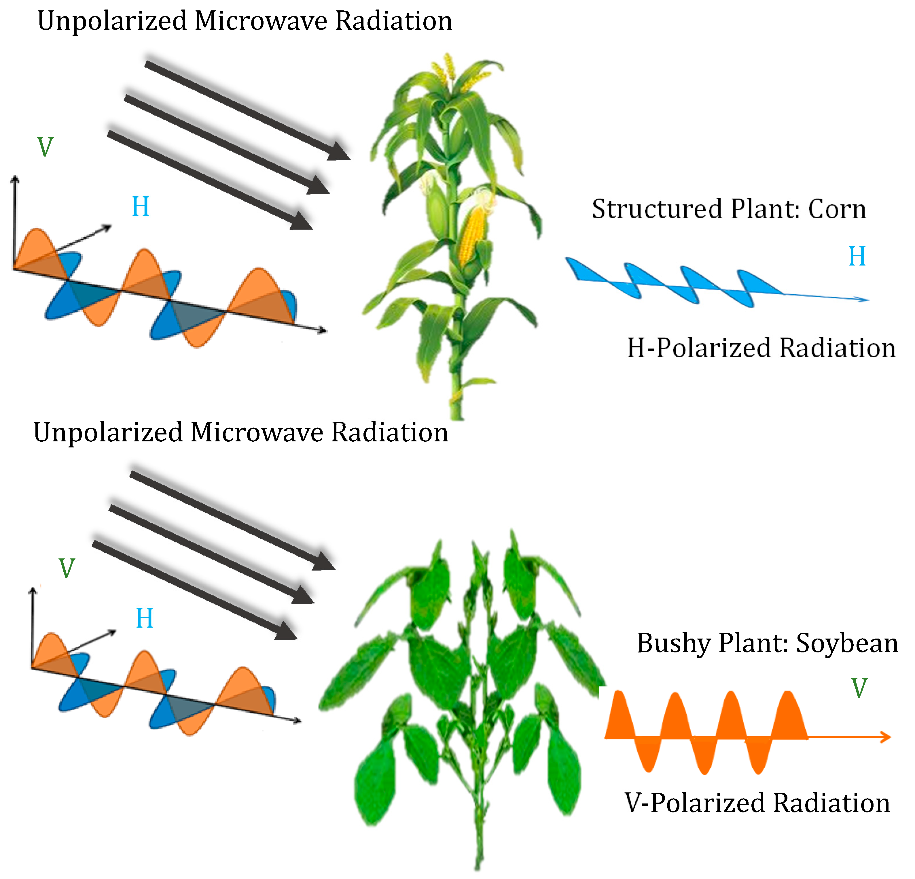
In canopies with vertical stalks, the attenuation will be smaller for horizontally polarized waves than vertically polarized waves except at a nadir incidence angle, where stalks are not visible and appear only as small randomly oriented disks (Figure 2). For a horizontally polarized incident wave, the electric field vector E is normal to the axis of the stalk at all incidence angles, and for a vertically polarized wave, E is parallel to stalk, thereby coupling strongly [77]. This difference will be significant mainly over vegetation that exhibits some preferential orientation such as vertical stalks noticed for tall grasses, grains, wheat, corn, maize, forest, etc. For vegetation with near horizontally oriented primary branches or broad leaf plants (soybean, bean, canola, sunflower, etc.), there is stronger attenuation for a horizontally polarized wave than vertically polarized waves. It is reasonable to assume that the absorption/scattering loss factor will be approximately polarization independent for canopy components whose sizes are much smaller than the wavelength of observation.
For example, for SMEX04 (Arizona), the vegetation is mainly shrub dominated (whitethorn acacia, creosote bush, etc.) covering two-thirds of the watershed, and grass (sideoats grama, lehmann lovegrass, etc.) occupying the rest with a total mean vegetation water content 0.087 kg/m2. Due to the low vegetation and primarily random vegetation structure, the sensitivity to vegetation variables is insignificant for this region temporally, at all support scales and polarizations (Figure 3). Similarly, the SGP97 region (Oklahoma), which is dominantly rangeland and has a significant occupation of winter wheat crops with a total mean vegetation water content of 0.323 kg/m2, shows the insignificant contribution of vegetation variables towards brightness temperature (V- and H-polarization) at all spatial scales (Figure 4). SMEX02 (Iowa) has a total mean vegetation water content of 1.9 kg/m2. At the 800 m scale, H-polarization was observed to be (~1–4%) more sensitive than V-polarization. With an increasing support scale, V-polarization was observed to be ~2% (at 1.6 km) and ~15% (at 12.8 km) more sensitive than H-polarization for vegetation water content (VWC) and vegetation structure (B) (Figure 5). Under IDW analysis, H-polarization was always temporally more sensitive than V-polarization to vegetation water content by ~2–3% and vegetation structure (B) by ~3–9%, except on DOY 188, where V- and H-polarization showed the same sensitivities (Figure 5). That is, at lower vegetation water content (DOY 178, 182) and a support scale of 800 m under linear upscaling and at all support scales under IDW where the heterogeneity in VWC is maintained, a higher sensitivity to VWC and B at H-polarization is noticed. For DOY 188, with higher vegetation water content and higher support scales under linear upscaling where the heterogeneity disappeared with support scales (moving towards extent mean value), a higher sensitivity to vegetation structure (B) at V-polarization is observed. This confirmed that there is a stronger coupling with plants exhibiting definite vertical structures, and the coupling increases with increasing vegetation water content and decreasing heterogeneity. The SMAPVEX12 region shows a wide variety of agricultural crops such as cereals, soybeans, canola, corn, etc., with a total mean vegetation content water of 1.4 kg/m2. Unlike in SMEX02, the sensitivity to vegetation structure (B) was always observed to be higher for H-polarization at all scales. We hypothesize that the amount of vegetation water content determines the sensitivity of H- and V-polarization to the B variable. To test the hypothesis, the analysis was conducted including pixels with higher vegetation water content than those observed within the SMAPVEX12 extent, which resulted in higher sensitivity to vegetation structure (B) at V-polarization. This may occur because with increasing VWC, the dielectric constant of vegetation also increases, thereby increasing the sensitivity to V-polarization due to stronger coupling, as mentioned earlier. Thus, vegetation variable ‘B’ is a complex function of plant geometry and vegetation water content.
3.2. Spatio-Temporal Scales in Different Hydroclimates
3.2.1. Semi-Arid (SMEX04) Hydroclimate
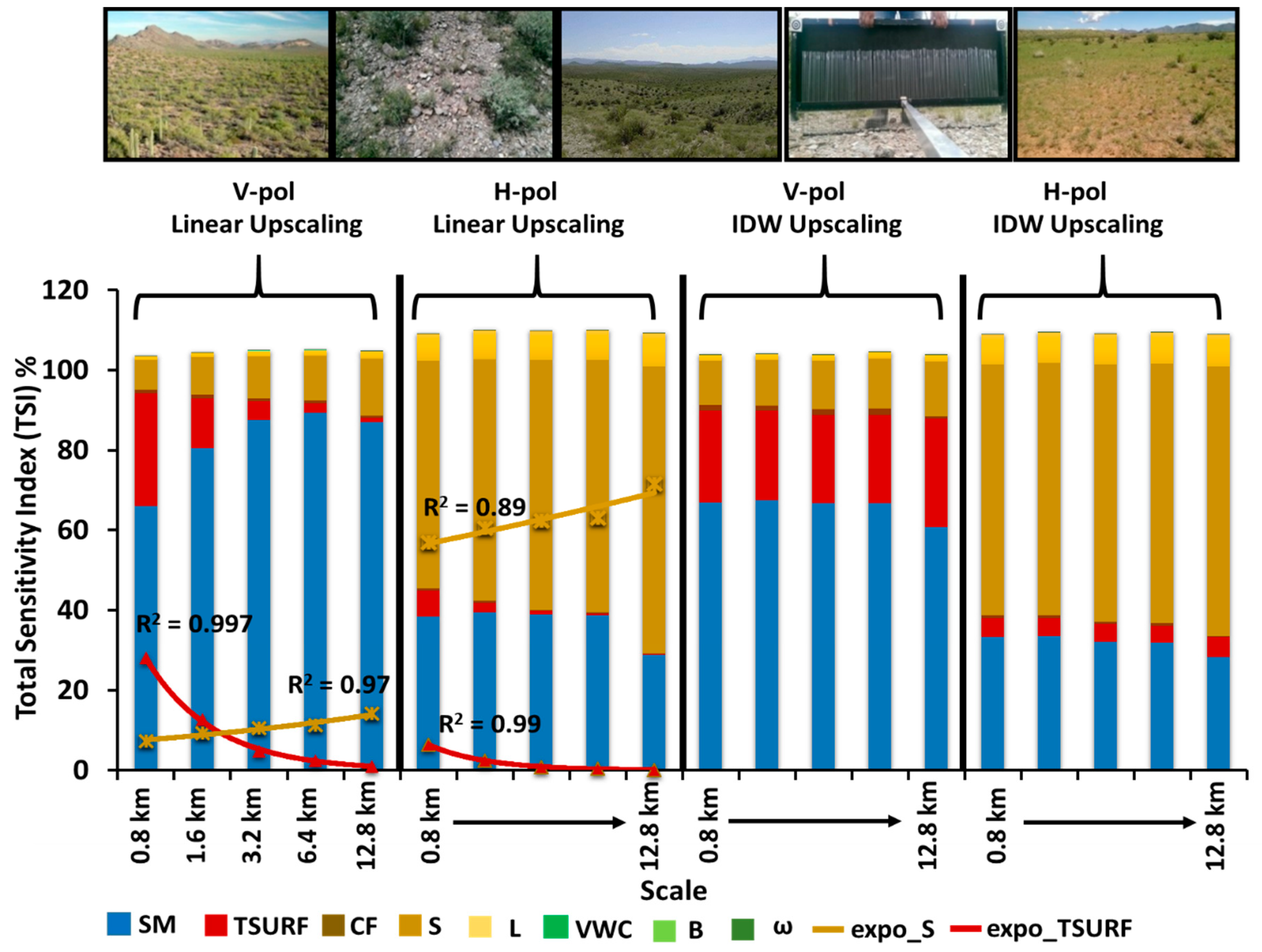
For semi-arid regions with low vegetation and lower evapotranspiration (lower latent heat flux and higher sensible heat flux), an increase in air and surface temperatures are observed, resulting in higher sensitivity to surface temperature. However, the heterogeneity in temperature is lost with upscaling due to lumped fluxes resulting in exponential (R2 = 0.99) decrease (increased) in sensitivity to surface temperature (RMS height, S) with support scale. A general decrease in R2 is noticed for the for H-pol, and this is observed across all hydroclimates, as noted in Figure 3. Due to the rocky topography of SMEX04 region, the observed surface roughness is highly random, emphasizing the higher sensitivity to RMS height (S), which increased from ~11% (~63%) to ~38% (~87%) for V-polarization (H-polarization), and correlation length (L) increased from ~1% (~7%) to ~5% (~10%). This is in contrast to SMAPVEX12 and SMEX02, where the surface roughness is more correlated due to regular agricultural practices resulting in higher sensitivity to correlation length (L) as well. The sensitivity to vegetation variables (VWC, B, and ω) and clay fractions are negligible across both polarizations (H and V), upscaling methods, and spatio-temporal scales.
3.2.2. Sub-Humid (SGP97) Hydroclimate
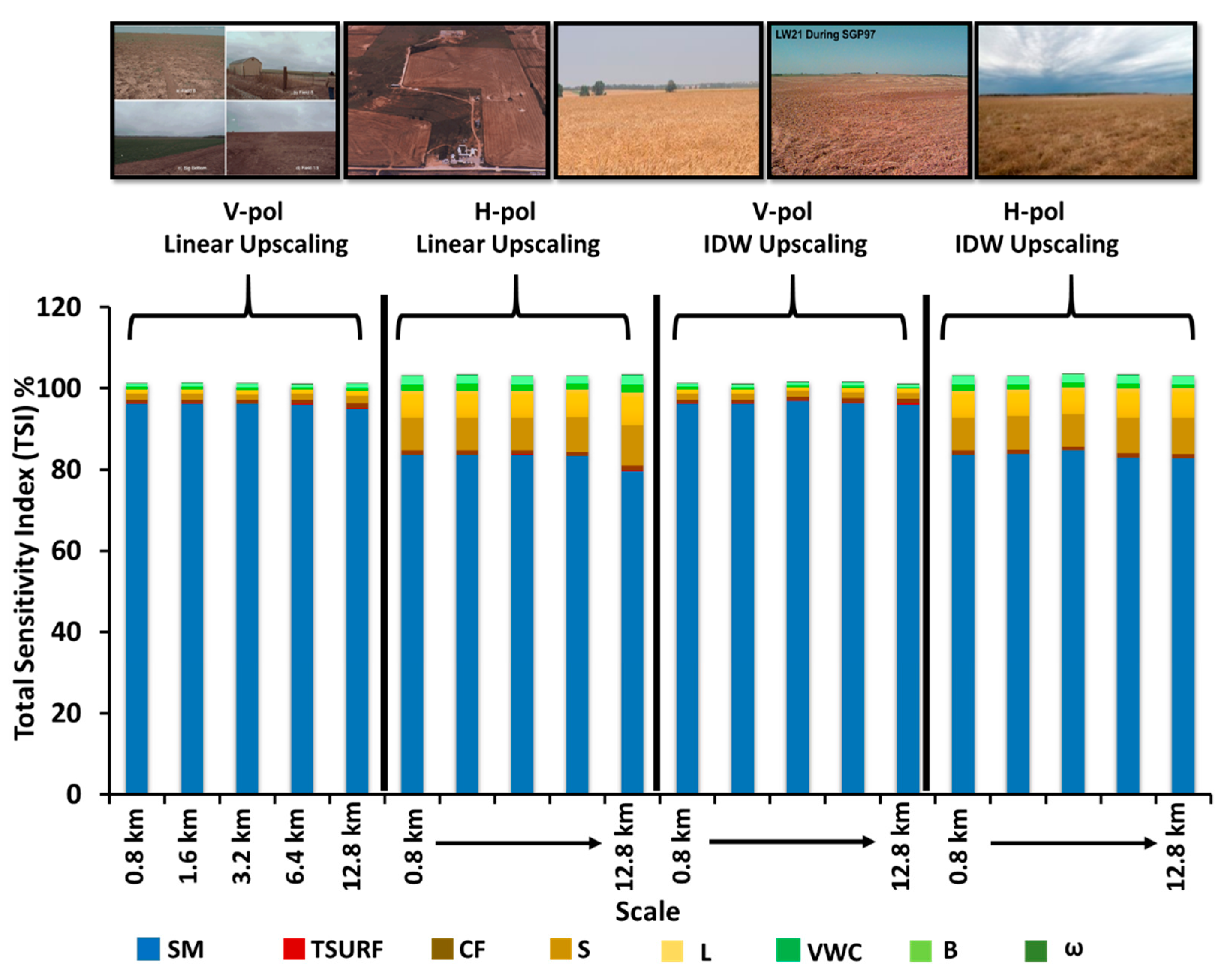
For a more natural landscape with low density biomass, as observed for SGP97, soil moisture is the most sensitive variable for V-polarization (H-polarization) ~96% (~83%) at all support scales under both linear and IDW upscaling. Due to the lower variability of roughness in SGP97 and lower biomass content, incorporating neighboring pixels via IDW or using linear upscaling did not influence the sensitivity measures with support scales. The sensitivity to land surface variables (clay, surface temperature, and scattering albedo) are insignificant (~1%) at V-polarization, whereas the sensitivity to surface roughness variables (S and L) at H-polarization are observed at ~8% each, and sensitivity to vegetation variables (VWC and B) are observed at ~2% each (Figure 4). To further explore the influence of varying extent, the analysis is repeated for a smaller extent over the Little Washita (LW) watershed. To maintain statistically significant data points, the upscaling is conducted only up to a 3.2 km support scale. Results indicated soil moisture (in both V- and H-polarization) to still be the most sensitive variable at all scales; however, its magnitude has decreased slightly to ~94% for V- polarization and ~80% for H- polarization. Sensitivity to the vegetation structure, (B) increased to ~4% and ~2% for H- and V-polarization, respectively, at a smaller extent than the sensitivities observed at a larger extent. This could be due to the increased attenuation caused by higher biomass content (~0.41 kg/m2) for a smaller extent than observed at a larger extent (SM ~0.14 v/v and VWC ~0.32 kg/m2).
3.2.3. Humid-Dfa (SMEX02) Hydroclimate
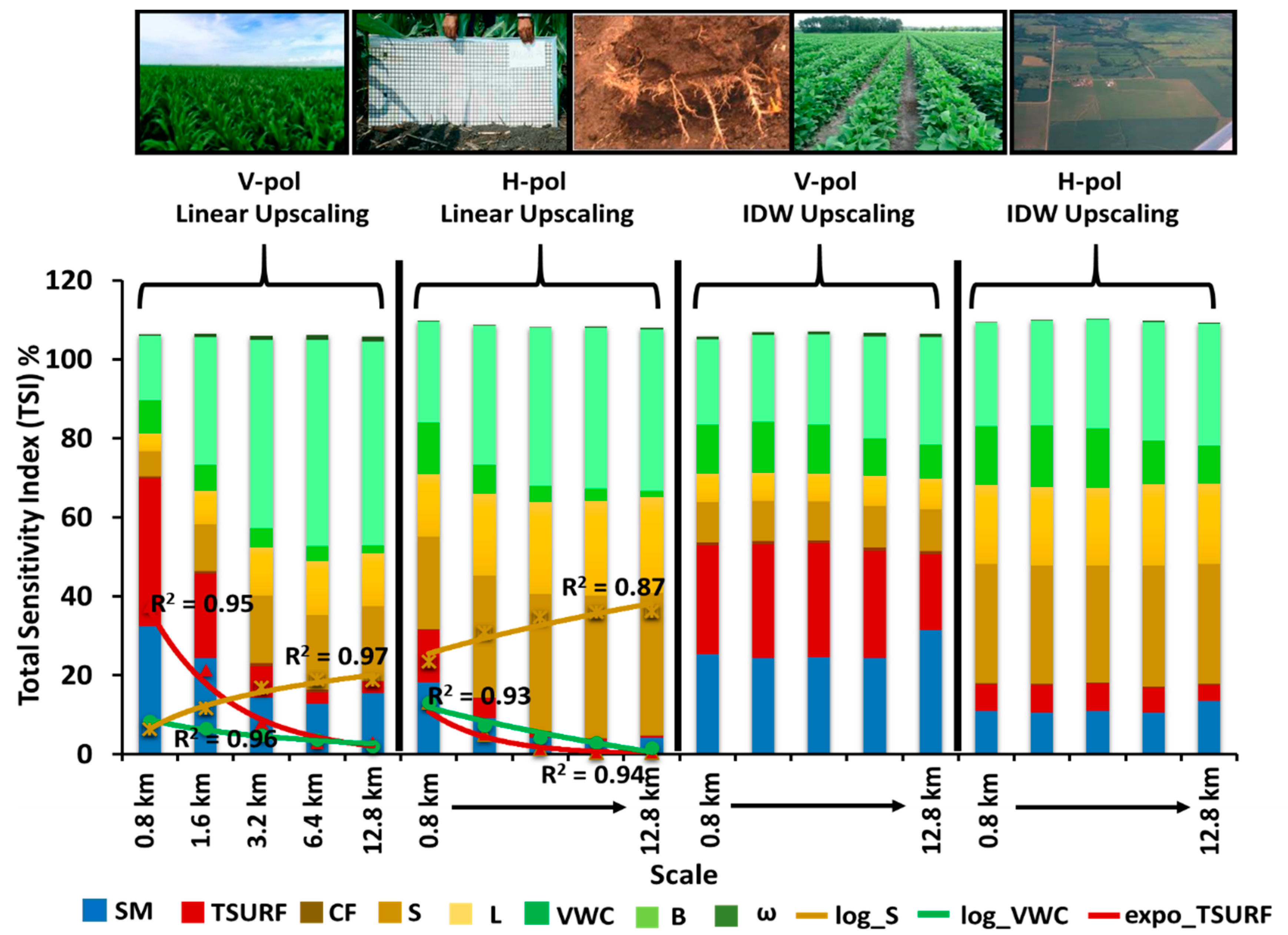
For SMEX02, the analysis is conducted for DOY 178, 182, 186, and 188, and the soil moisture sensitivity at 800 m followed a similar field scale pattern as observed in Neelam and Mohanty (2015) [26]. Unlike SMEX04 and SGP97, the mean sensitivity to soil moisture across sampling days is ~28% and ~13% for V- and H-polarization, respectively, at 800 m, which decreased to ~8% and ~1% at 6.4 km, and increased by ~1–2% at 12.8 km (Figure 5). Among other land surface variables, sensitivity to surface temperature followed a decreasing exponential function (R2 = ~0.95) and nearly disappeared at 1.6 km for H- and at 3.2 km for V-polarization. On the other hand, the sensitivity to surface roughness variables (S and L) followed a logarithmic function (R2 = ~0.97) with an increasing support scale. Similarly, vegetation water content (VWC) and vegetation structure (B) followed a decreasing (R2 = 0.96) and increasing logarithmic function. This is because of the greater variability in surface roughness and vegetation variables observed, particularly for the anthropogenically-modified region such as SMEX02. Thus, the impact of these variables is observed longer with a support scale following a logarithmic function, compared to the surface temperature that followed an exponential function. Under IDW upscaling, the sensitivity to land surface variables with support scales changed by ~1–2%. Sensitivity to variables such as soil moisture, surface temperature, and surface roughness remained uniform until 6.4 km, which later decreased by ~2% for soil moisture and surface temperature, and increased for surface roughness by ~2% at 12.8 km. The uniformity in sensitivity to these variables until 6.4 km under IDW is similar to the reasons explained above. However, for a selected extent, the variability in some land surface variables attains saturation at a certain scale (6.4 km), resulting in a decrease in sensitivity to those land surface variables upon further upscaling. The support scale at which this saturation is attained is dependent on the heterogeneity and extent of the analysis. The sensitivity to vegetation water content remained uniform until 3.2 km and decreased ~1% with an increasing support scale, and sensitivity to vegetation structure (B) increased linearly (R2 =0.98) by ~6% with the scale. The sensitivity to clay fraction and albedo remained negligible under IDW and linear upscaling. Except for DOY 178, which was a relatively dry day, the sensitivity to clay fraction increased to ~3% at V-polarization and ~1% at H-polarization until 3.2 km.
It is important to note that we discuss only the total sensitivity indices (TSI) of the land surface variables. The increased sensitivity of a variable may also be due to increased interaction effects such as (S,B), (S,VWC), (S,SM), (L,VWC), and (SM,B) with growing vegetation (increased interception and scattering) [26]. This may also be one of the contributing factors of the high sensitivity to surface roughness (S and L) and vegetation structure (B). The sensitivity to scattering albedo is observed to be negligible at all scales.
3.2.4. Humid-Dfb (SMAPVEX12) Hydroclimate
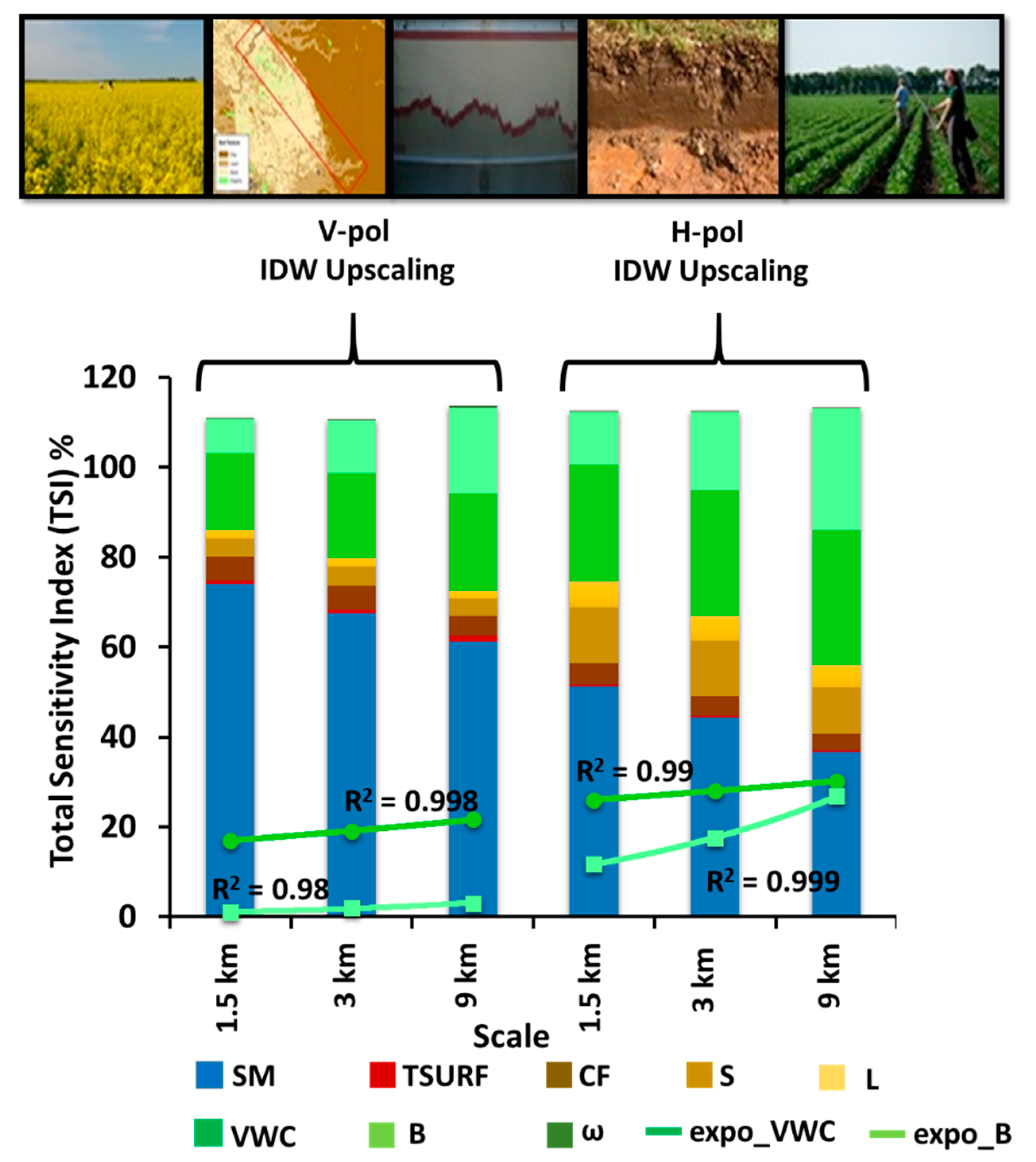
The SMAPVEX12 region observed lower biomass content and a wide heterogeneity in soil moisture due to a more gradual variability in sensitivity to land surface variables being noticed, unlike SMEX02. To maintain statistically significant sample points, the upscaling is conducted from 1.5 km to 9 km only. The sensitivity of V-polarization (H-polarization) to soil moisture showed ~74% (~52%) at 1.5 km, which decreased to ~61% (~35%) at 9 km (Figure 6). The sensitivity to clay fraction remained uniform (~6%) spatio-temporally for both V- and H-polarization. A relatively high sensitivity to clay in SMAPVEX12, unlike other regions, is due to a wide heterogeneity (~5% to ~65%) in clay fraction observed in this region. The sensitivity to surface roughness variables (S and L) is uniform at ~2–4% at all scales, unlike in SMEX02, where they increased with scale. This may also be due to higher surface roughness measured for SMEX02 than SMAPVEX12. The sensitivity to vegetation structure and vegetation water content increased exponentially (R2 = 0.99) with scale. It is noteworthy that the sensitivity to VWC slightly increased with scale.
3.3. Upscaling and Environmental Heterogeneity
The largest up-scaling effects are observed for scenes with high heterogeneity, i.e., with strong gradients in land surface variables. The differences between the two (linear and IDW) upscaling methods are, therefore, more prominent in heterogeneous environments. A high correlation is observed between spatial heterogeneity in soil moisture and density of vegetation [23,44]. Thus, we classify the hydroclimates as heterogeneous and homogeneous environments based on biomass density. This also complements Mo et al. (1982) [40] and Wigneron et al. (1995) [78], who suggested that the total amount of biomass within the pixel is important in affecting the microwave response.
3.3.1. Homogeneous Environment (Sub-Humid and Semi-Arid)
SGP’97 (Sub-Humid) and SMEX04 (Semi-Arid) are more natural landscapes composed mainly of grasslands and shrubs, with low biomass content. For SGP97, a very small percentage of higher order interactions are observed, ~1% for V-polarization and ~3% for H-polarization. SMEX04 observed higher order interactions of ~5% for V-polarization and ~9% for H-polarization. Due to the rough topography of SMEX04, a higher sensitivity to roughness variables (S and L) for H-polarization is observed, which also led to increased higher order interactions than SGP97. Because of higher sensitivity to soil moisture and nearly linear (additive) behavior of the radiative transfer model, these regions can be classified as homogenous environments. Due to the homogeneous environment, we do not observe large variabilities in sensitivity measures between linear and non-linear (IDW) upscaling methods (Figure 3 and Figure 4). This allows the land surface variables to be scaled linearly, which is also consistent with studies of Drusch et al. (1999) [68] and Crow et al. (2000) [79]. Under homogeneous environments, SMEX04 and SGP97 can further be classified as energy rich and water rich environments, respectively. SMEX04 that observed a total mean soil moisture of ~0.07 v/v and higher surface temperatures of ~319 K is classified as the energy rich environment, and SGP97 that observed a relatively higher total mean soil moisture of ~0.15 v/v and lower surface temperatures of ~298 K can be classified as a water rich environment. For a homogeneous water rich environment, the sensitivity to land surface variables did not vary with either the support scale or the upscaling methods, and varied only by small percentages due to polarization differences. The sensitivity to land surface variables under homogeneous energy rich environments followed an exponential function with support scale and attained uniformity by ~3.2 km, emphasizing the linearity/homogeneity of the region.
3.3.2. Heterogeneous Environment (Humid Dfa and Humid Dfb)
SMEX02 (Humid Dfa) and SMAPVEX12 (Humid Dfb) are agricultural landscapes with a wide range of biomass content and observe tillage practices on a regular basis. In these regions, the sensitivity to land surface variables are complex and exhibited considerable higher order interactions (non-linearities). SMAPVEX12 observed higher order interactions of ~6% for V-polarization and ~10% for H-polarization, whereas SMEX02 observed ~10% for V-polarization and ~13% for H-polarization. Because of lower sensitivity to soil moisture and higher non-linear behavior of the radiative transfer model, these regions can be classified as heterogeneous environments. Due to the heterogeneous environment, there is a significant gradient observed in the sensitivity of land surface variables as they are upscaled linearly from 800 m to 12.8 km. However, as they are upscaled non-linearly, the gradient in the sensitivity measures decreases (Figure 5 and Figure 6). Under heterogeneous environments, SMEX02 and SMAPVEX12 can further be classified as energy rich and water rich environments, respectively. SMEX02, which observed mean soil moisture ~0.19 v/v and mean surface temperatures of ~315 K, is classified as an energy rich environment. On the other hand, SMAPVEX12, which observed a relatively higher mean soil moisture ~0.25 v/v and lower mean surface temperatures ~290 K, is classified as water rich environment. For a heterogeneous water rich environment (SMAPVEX12), the sensitivity to land surface variables followed an exponential function with a support scale, and for a heterogeneous energy rich environment (SMEX02), the sensitivity to land surface variables followed a logarithmic function emphasizing the non-linearity/interactions of the region. Therefore, under heterogeneous environments, the upscaling method also determined the sensitivity to land surface variables.
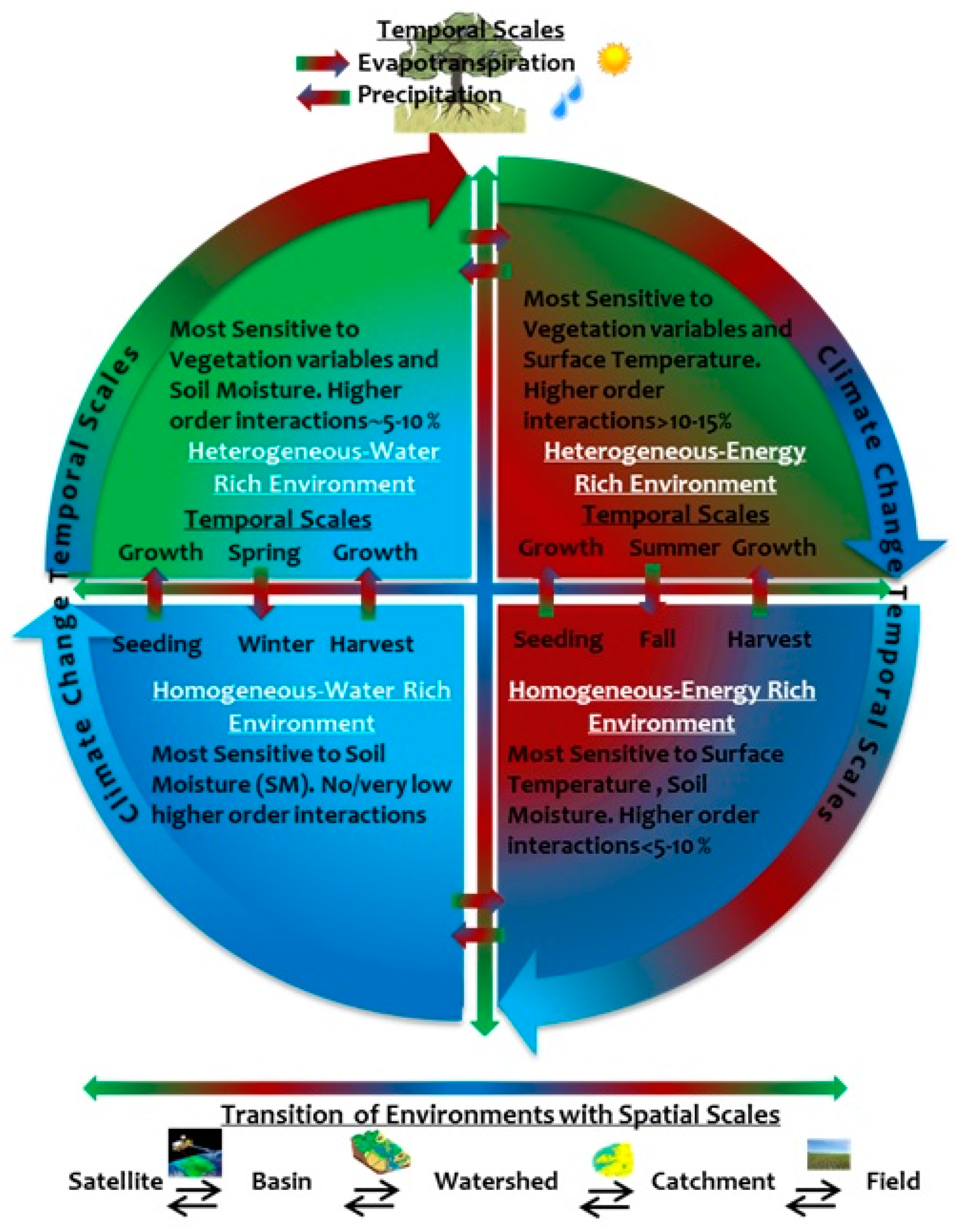
In this study, a comprehensive framework is proposed based on the preliminary work presented by Neelam and Mohanty (2015) [26] (Figure 7), where the regions can primarily be classified as homogenous and heterogeneous environments based on density and heterogeneity in biomass. Each of these environments can further be classified as water and energy rich environments. The transition from homogenous to heterogeneous, energy rich to water rich, and vice versa, can occur through spatial parameters (extent and support), time (day, month, seasonality, etc.), and hydroclimates. For example, with a gradual increase in spatial scale (support, extent, and spacing) there will be a gradual change in land-cover/land-use, thereby changing heterogeneity in land surface variables captured with a varying spatial scale. Similarly, heterogeneity in land surface variables changes with temporal scales. For example, activities at monthly temporal scales such as seeding, irrigation, crop growth, harvesting, etc., and at seasonal scales such as spring, summer, fall, etc., effects heterogeneity in biomass, water, temperature, etc. Thus, the transitioning of the environments occurs through spatio-temporal scales, thereby changing the heterogeneity in the land surface variables and their sensitivities to the soil moisture retrieval algorithm.
4. Conclusions
A comprehensive sensitivity analysis to study radiative transfer model using spatial maps is conducted for various field campaigns in multiple hydroclimates. The primary contribution of this work is to demonstrate how the sensitivity to the spatial maps of land surface variables change under various hydroclimates (Arizona, Oklahoma, Iowa, and Winnipeg) and evolving scales (0.8 km, 1.6 km, 3.2 km, 6.4 km, and 12.8 km) for a given extent. The impact of non-linear upscaling is illustrated by the comparison between linear and inverse distance weighted methods. The analysis resulted in environment-specific most sensitive variables: SM in homogeneous, and VWC and B in heterogeneous environments. Though the magnitude of sensitivity varied temporally, the ranking among the variables did not change within the study period. In the case of homogeneous landscapes or largely undisturbed natural environments, the sensitivity of TB to variables remained nearly uniform or followed an exponential function with support scales. Under higher heterogeneity, the TB sensitivity to vegetation and roughness followed a logarithmic function with an increasing support scale. Surface temperature always followed an exponential function under all conditions. The upscaling methods play a significant role in representing non-linear effects of heterogeneous landscapes, as processes and variables change their significance with scale. It is recommended that the most sensitive variables to TB (H- or V-) should be upscaled using non-linear (e.g., IDW) methods to preserve spatial heterogeneity, and this is especially important under heterogeneous environments. The study emphasized that the observed heterogeneity and upscaling method will determine the sensitivity to land surface variables. This study is particularly relevant in order to establish the significant variables that can be used for downscaling and upscaling TB algorithms to various scales and under heterogeneous landscapes.
The analysis assumed independence among the input variables, which might not be true under natural environments. However, there are very limited studies in the past that have established a correlation among land surface variables. Also, the study assumes the range of variability in the vegetation parameters and scattering albedo to be constant at all scales. Since there are no means to ascertain how those vary with scale, this assumption may introduce uncertainties. The future scope of this work can include analyzing the sensitivity of correlated land surface variables and its development with hydroclimates and scales.
Author Contributions
M.N. and B.P.M. designed research; M.N. performed research and analysis; M.N. and B.P.M. wrote the paper. All authors have read and agreed to the published version of the manuscript.
Funding
This research was funded by Schlumberger Faculty for Future Fellowship and NASA Grant NNX16AQ58G.
Acknowledgments
We acknowledge the support of the Schlumberger Faculty for Future Fellowship and thank all the students, scientists, and volunteers who participated in the various soil moisture campaigns and collected valuable data. The data for Oklahoma, Arizona, Iowa and Winnipeg, Canada used in this study can be accessed from the links provided below http://nsidc.org/data/amsr_validation/soil_moisture/index.html.
Conflicts of Interest
The authors declare no conflict of interest.
Appendix A
Consider a model defined as Y = f(X), where Y is the output, X = ( are k independent inputs, and f is the model function. If all the factors X are allowed to vary over their range of uncertainty, then the corresponding uncertainty of the model output Y is defined by its unconditional variance V(Y). The input factors are ranked based on the amount of variance removed from the output when we learn the true value of a given input factor Xi. That is, ) would be the resulting conditional variance as it is fixed to its true value taken over all (all factors but ). However, the true value is unknown for each . Hence, an average of ) measured over all possible values will remove the dependence of , thereby resulting in Using the following property (Mood et al., 1950) [80],
Thus, a small or a large will imply that Xi is an important factor. The conditional variance is the first-order (e.g., additive) effect of Xi on Y and the associated first-order sensitivity index of Xi on Y measure, which is written as while is customarily called the residual. As such, is a number always between 0 and 1. Sobol [48] introduced the decomposition of model function f into summands of increasing dimensionality:
In Equation (2), each individual term is a square integrable over the domain of existence and is mutually orthogonal [50]. These functions are associated with partial variances through:
and so on for higher order terms. Assuming all inputs to be independent, these terms are linked as: Dividing both sides of the equation by unconditional variance V(Y), we obtain;
where First Order Sensitivity Index Second Order Sensitivity Index the amount of variance of Y explained by the interaction of the factors Xi and Xj (i.e., sensitivity to Xi and Xj not expressed in individual Xi and Xj); Total Sensitivity Index ; this accounts for all the contributions to the output variation due to factor Xi (i.e., first-order index plus all its interactions). can also be defined by decomposing the output variance V(Y), in terms of main effect and residual, conditioning with respect to all factors but one, i.e., . The unconditional variance can be rewritten as: , and dividing both sides by unconditional variance results in: .
In other words, index is defined as a summation of the main, second, and higher order effects, which involves the evaluation over a full range of parameter space. For further details on the computation of sensitivity indices, please refer to Saltelli (2002).
References
- Moran, M.S.; Doorn, B.; Escobar, V.; Brown, M.E. Connecting NASA science and engineering with earth science applications. J. Hydrometeorol. 2015, 16, 473–483. [Google Scholar] [CrossRef] [Green Version]
- Mecklenburg, S.; Drusch, M.; Kaleschke, L.; Rodriguez-Fernandez, N.; Reul, N.; Kerr, Y.; Font, J.; Martin-Neira, M.; Oliva, R.; Daganzo-Eusebio, E. ESA’s Soil Moisture and Ocean Salinity mission: From science to operational applications. Remote Sens. Environ. 2016, 180, 3–18. [Google Scholar] [CrossRef]
- Spencer, M.; Wheeler, K.; White, C.; West, R.; Piepmeier, J.; Hudson, D.; Medeiros, J. The Soil Moisture Active Passive (SMAP) mission L-band radar/radiometer instrument. In Proceedings of the 2010 IEEE International Geoscience and Remote Sensing Symposium, Honolulu, HI, USA, 25–30 July 2010; pp. 3240–3243. [Google Scholar]
- Merlin, O.; Rudiger, C.; Al Bitar, A.; Richaume, P.; Walker, J.P.; Kerr, Y.H. Disaggregation of SMOS soil moisture in Southeastern Australia. IEEE Trans. Geosci. Remote Sens. 2012, 50, 1556–1571. [Google Scholar] [CrossRef] [Green Version]
- Das, N.N.; Entekhabi, D.; Njoku, E.G.; Shi, J.J.; Johnson, J.T.; Colliander, A. Tests of the SMAP combined radar and radiometer algorithm using airborne field campaign observations and simulated data. IEEE Trans. Geosci. Remote Sens. 2013, 52, 2018–2028. [Google Scholar] [CrossRef]
- Wu, X.; Walker, J.P.; Das, N.N.; Panciera, R.; Rüdiger, C. Evaluation of the SMAP brightness temperature downscaling algorithm using active–passive microwave observations. Remote Sens. Environ. 2014, 155, 210–221. [Google Scholar] [CrossRef]
- Molero, B.; Merlin, O.; Malbéteau, Y.; Al Bitar, A.; Cabot, F.; Stefan, V.; Kerr, Y.; Bacon, S.; Cosh, M.H.; Bindlish, R. SMOS disaggregated soil moisture product at 1 km resolution: Processor overview and first validation results. Remote Sens. Environ. 2016, 180, 361–376. [Google Scholar] [CrossRef]
- Piles, M.; Entekhabi, D.; Camps, A. A change detection algorithm for retrieving high-resolution soil moisture from SMAP radar and radiometer observations. IEEE Trans. Geosci. Remote Sens. 2009, 47, 4125–4131. [Google Scholar] [CrossRef]
- Piles, M.; Camps, A.; Vall-Llossera, M.; Corbella, I.; Panciera, R.; Rudiger, C.; Kerr, Y.H.; Walker, J. Downscaling SMOS-derived soil moisture using MODIS visible/infrared data. IEEE Trans. Geosci. Remote Sens. 2011, 49, 3156–3166. [Google Scholar] [CrossRef]
- Shin, Y.; Mohanty, B.P. Development of a deterministic downscaling algorithm for remote sensing soil moisture footprint using soil and vegetation classifications. Water Resour. Res. 2013, 49, 6208–6228. [Google Scholar] [CrossRef]
- Song, C.; Jia, L.; Menenti, M. Retrieving high-resolution surface soil moisture by downscaling AMSR-E brightness temperature using MODIS LST and NDVI data. IEEE J. Sel. Top. Appl. Earth Obs. Remote Sens. 2013, 7, 935–942. [Google Scholar] [CrossRef]
- Djamai, N.; Magagi, R.; Goita, K.; Merlin, O.; Kerr, Y.; Walker, A. Disaggregation of SMOS soil moisture over the Canadian Prairies. Remote Sens. Environ. 2015, 170, 255–268. [Google Scholar] [CrossRef] [Green Version]
- Western, A.W.; Blöschl, G. On the spatial scaling of soil moisture. J. Hydrol. 1999, 217, 203–224. [Google Scholar] [CrossRef]
- Van de Griend, A.A.; Wigneron, J.-P.; Waldteufel, P. Consequences of surface heterogeneity for parameter retrieval from 1.4-GHz multiangle SMOS observations. IEEE Trans. Geosci. Remote Sens. 2003, 41, 803–811. [Google Scholar] [CrossRef]
- Dorigo, W.A.; Scipal, K.; Parinussa, R.M.; Liu, Y.Y.; Wagner, W.; De Jeu, R.A.; Naeimi, V. Error characterisation of global active and passive microwave soil moisture datasets. Hydrol. Earth Syst. Sci. 2010, 14, 2605. [Google Scholar] [CrossRef] [Green Version]
- Merlin, O.; Malbéteau, Y.; Notfi, Y.; Bacon, S.; Khabba, S.E.-R.S.; Jarlan, L. Performance metrics for soil moisture downscaling methods: Application to DISPATCH data in central Morocco. Remote Sens. 2015, 7, 3783–3807. [Google Scholar] [CrossRef] [Green Version]
- Njoku, E.G.; Entekhabi, D. Passive microwave remote sensing of soil moisture. J. Hydrol. 1996, 184, 101–129. [Google Scholar] [CrossRef]
- Western, A.W.; Grayson, R.B.; Blöschl, G. Scaling of soil moisture: A hydrologic perspective. Annu. Rev. Earth Planet. Sci. 2002, 30, 149–180. [Google Scholar] [CrossRef] [Green Version]
- Entekhabi, D.; Njoku, E.G.; O’Neill, P.E.; Kellogg, K.H.; Crow, W.T.; Edelstein, W.N.; Entin, J.K.; Goodman, S.D.; Jackson, T.J.; Johnson, J.; et al. The Soil Moisture Active Passive (SMAP) Mission. Proc. IEEE 2010, 98, 704–716. [Google Scholar] [CrossRef]
- Ryu, D.; Famiglietti, J.S. Multi-scale spatial correlation and scaling behavior of surface soil moisture. Geophys. Res. Lett. 2006, 33. [Google Scholar] [CrossRef] [Green Version]
- Gaur, N.; Mohanty, B.P. Evolution of physical controls for soil moisture in humid and subhumid watersheds. Water Resour. Res. 2013, 49, 1244–1258. [Google Scholar] [CrossRef]
- Gaur, N.; Mohanty, B.P. Land-surface controls on near-surface soil moisture dynamics: Traversing remote sensing footprints. Water Resour. Res. 2016, 52, 6365–6385. [Google Scholar] [CrossRef] [Green Version]
- Lakhankar, T.; Ghedira, H.; Temimi, M.; Azar, A.E.; Khanbilvardi, R. Effect of land cover heterogeneity on soil moisture retrieval using active microwave remote sensing data. Remote Sens. 2009, 1, 80–91. [Google Scholar] [CrossRef] [Green Version]
- Roy, S.K.; Rowlandson, T.L.; Berg, A.A.; Champagne, C.; Adams, J.R. Impact of sub-pixel heterogeneity on modelled brightness temperature for an agricultural region. Int. J. Appl. Earth Obs. Geoinf. 2016, 45, 212–220. [Google Scholar] [CrossRef]
- Burke, E.J.; Simmonds, L.P. Effects of sub-pixel heterogeneity on the retrieval of soil moisture from passive microwave radiometry. Int. J. Remote Sens. 2003, 24, 2085–2104. [Google Scholar] [CrossRef]
- Neelam, M.; Mohanty, B.P. Global sensitivity analysis of the radiative transfer model. Water Resour. Res. 2015, 51, 2428–2443. [Google Scholar] [CrossRef]
- Saint-Geours, N.; Lavergne, C.; Bailly, J.-S.; Grelot, F. Sensitivity analysis of spatial models using geostatistical simulation. In Proceedings of the Mathematical Geosciences at the Crossroads of Theory and Practice—IAMG 2011 Conference, Salzburg, Austria, 5–9 September 2011. [Google Scholar]
- Sarrazin, F.; Pianosi, F.; Wagener, T. Global Sensitivity Analysis of environmental models: Convergence and validation. Environ. Model. Softw. 2016, 79, 135–152. [Google Scholar] [CrossRef] [Green Version]
- Pianosi, F.; Beven, K.; Freer, J.; Hall, J.W.; Rougier, J.; Stephenson, D.B.; Wagener, T. Sensitivity analysis of environmental models: A systematic review with practical workflow. Environ. Model. Softw. 2016, 79, 214–232. [Google Scholar] [CrossRef]
- Crosetto, M.; Tarantola, S.; Saltelli, A. Sensitivity and uncertainty analysis in spatial modelling based on GIS. Agric. Ecosyst. Environ. 2000, 81, 71–79. [Google Scholar] [CrossRef]
- Cosh, M.H.; Jackson, T.J.; Moran, S.; Bindlish, R. Temporal persistence and stability of surface soil moisture in a semi-arid watershed. Remote Sens. Environ. 2008, 112, 304–313. [Google Scholar] [CrossRef]
- Jackson, T.J.; Cosh, M.H.; Bindlish, R.; Starks, P.J.; Bosch, D.D.; Seyfried, M.; Goodrich, D.C.; Moran, M.S.; Du, J. Validation of Advanced Microwave Scanning Radiometer Soil Moisture Products. IEEE Trans. Geosci. Remote Sens. 2010, 48, 4256–4272. [Google Scholar] [CrossRef]
- McNairn, H.; Jackson, T.J.; Wiseman, G.; Belair, S.; Berg, A.; Bullock, P.; Colliander, A.; Cosh, M.H.; Kim, S.-B.; Magagi, R. The soil moisture active passive validation experiment 2012 (SMAPVEX12): Prelaunch calibration and validation of the SMAP soil moisture algorithms. IEEE Trans. Geosci. Remote Sens. 2014, 53, 2784–2801. [Google Scholar] [CrossRef]
- Peel, M.C.; Finlayson, B.L.; McMahon, T.A. Updated world map of the Köppen-Geiger climate classification. Hydrol. Earth Syst. Sci. Discuss. 2007, 4, 439–473. [Google Scholar] [CrossRef] [Green Version]
- Jackson, T.J.; Le Vine, D.M.; Hsu, A.Y.; Oldak, A.; Starks, P.J.; Swift, C.T.; Isham, J.D.; Haken, M. Soil moisture mapping at regional scales using microwave radiometry: The Southern Great Plains Hydrology Experiment. IEEE Trans. Geosci. Remote Sens. 1999, 37, 2136–2151. [Google Scholar] [CrossRef] [Green Version]
- Jacobs, J.M.; Mohanty, B.P.; Hsu, E.-C.; Miller, D. SMEX02: Field scale variability, time stability and similarity of soil moisture. Remote Sens. Environ. 2004, 92, 436–446. [Google Scholar] [CrossRef]
- Bindlish, R.; Jackson, T.J.; Gasiewski, A.J.; Klein, M.; Njoku, E.G. Soil moisture mapping and AMSR-E validation using the PSR in SMEX02. Remote Sens. Environ. 2006, 103, 127–139. [Google Scholar] [CrossRef]
- Yilmaz, M.T.; Hunt, E.R.; Jackson, T.J. Remote sensing of vegetation water content from equivalent water thickness using satellite imagery. Remote Sens. Environ. 2008, 112, 2514–2522. [Google Scholar] [CrossRef]
- Colliander, A.; Njoku, E.G.; Jackson, T.J.; Chazanoff, S.; McNairn, H.; Powers, J.; Cosh, M.H. Retrieving soil moisture for non-forested areas using PALS radiometer measurements in SMAPVEX12 field campaign. Remote Sens. Environ. 2016, 184, 86–100. [Google Scholar] [CrossRef]
- Mo, T.; Choudhury, B.J.; Schmugge, T.J.; Wang, J.R.; Jackson, T.J. A model for microwave emission from vegetation-covered fields. J. Geophys. Res. Ocean. 1982, 87, 11229–11237. [Google Scholar] [CrossRef]
- Jackson, T.J.; Chen, D.; Cosh, M.; Li, F.; Anderson, M.; Walthall, C.; Doriaswamy, P.; Hunt, E.R. Vegetation water content mapping using Landsat data derived normalized difference water index for corn and soybeans. Remote Sens. Environ. 2004, 92, 475–482. [Google Scholar] [CrossRef]
- Jackson, T.J.; Schmugge, T.J. Vegetation effects on the microwave emission of soils. Remote Sens. Environ. 1991, 36, 203–212. [Google Scholar] [CrossRef]
- Ulaby, F.T.; Razani, M.; Dobson, M.C. Effects of Vegetation Cover on the Microwave Radiometric Sensitivity to Soil Moisture. IEEE Trans. Geosci. Remote Sens. 1983, GE-21, 51–61. [Google Scholar] [CrossRef]
- Said, S.; Kothyari, U.C.; Arora, M.K. Vegetation effects on soil moisture estimation from ERS-2 SAR images. Hydrol. Sci. J. 2012, 57, 517–534. [Google Scholar] [CrossRef]
- Brunfeldt, D.R.; Ulaby, F.T. Microwave emission from row crops. IEEE Trans. Geosci. Remote Sens. 1986, GE-24, 353–359. [Google Scholar] [CrossRef]
- Neelam, M.; Colliander, A.; Mohanty, B.P.; Cosh, M.H.; Misra, S.; Jackson, T.J. Multiscale Surface Roughness for Improved Soil Moisture Estimation. IEEE Trans. Geosci. Remote Sens. 2020, 1–13. [Google Scholar] [CrossRef]
- O’Neill, P.; Chan, S.; Njoku, E.; Jackson, T.; Bindlish, R. Algorithm theoretical basis document (ATBD): L2 & L3 radiometer soil moisture (Passive) data products. Smap Proj. Rev. A 2014. [Google Scholar]
- Sobol, I.M. Sensitivity estimates for nonlinear mathematical models. Math. Model. Comput. Exp. 1993, 1, 407–414. [Google Scholar]
- Saltelli, A. Making best use of model evaluations to compute sensitivity indices. Comput. Phys. Commun. 2002, 145, 280–297. [Google Scholar] [CrossRef]
- Saltelli, A.; Ratto, M.; Andres, T.; Campolongo, F.; Cariboni, J.; Gatelli, D.; Saisana, M.; Tarantola, S. Global sensitivity analysis: The primer; John Wiley & Sons: Hoboken, NJ, USA, 2008; ISBN 0-470-72517-6. [Google Scholar]
- Saltelli, A.; Ratto, M.; Tarantola, S.; Campolongo, F. Sensitivity analysis for chemical models. Chem. Rev. 2005, 105, 2811–2828. [Google Scholar] [CrossRef]
- Saltelli, A.; Annoni, P.; Azzini, I.; Campolongo, F.; Ratto, M.; Tarantola, S. Variance based sensitivity analysis of model output. Design and estimator for the total sensitivity index. Comput. Phys. Commun. 2010, 181, 259–270. [Google Scholar] [CrossRef]
- Choudhury, B.J.; Ahmed, N.U.; Idso, S.B.; Reginato, R.J.; Daughtry, C.S.T. Relations between evaporation coefficients and vegetation indices studied by model simulations. Remote Sens. Environ. 1994, 50, 1–17. [Google Scholar] [CrossRef]
- Efron, B.; Tibshirani, R. An Introduction to the Bootstrap; CRC Press: Boca Raton, FL, USA, 1993; Volume 57. [Google Scholar]
- Blöschl, G. Scaling issues in snow hydrology. Hydrol. Process. 1999, 13, 2149–2175. [Google Scholar] [CrossRef]
- Blöschl, G.; Sivapalan, M. Scale issues in hydrological modelling: A review. Hydrol. Process. 1995, 9, 251–290. [Google Scholar] [CrossRef]
- Raupach, M.R.; Finnigan, J.J. Scale issues in boundary-layer meteorology: Surface energy balances in heterogeneous terrain. Hydrol. Process. 1995, 9, 589–612. [Google Scholar] [CrossRef]
- Xie, J.; Liu, T.; Wei, P.; Jia, Y.; Luo, C. Ecological application of wavelet analysis in the scaling of spatial distribution patterns of Ceratoides ewersmanniana. Acta Ecol. Sin. 2007, 27, 2704–2714. [Google Scholar] [CrossRef]
- Malenovský, Z.; Bartholomeus, H.M.; Acerbi-Junior, F.W.; Schopfer, J.T.; Painter, T.H.; Epema, G.F.; Bregt, A.K. Scaling dimensions in spectroscopy of soil and vegetation. Int. J. Appl. Earth Obs. Geoinf. 2007, 9, 137–164. [Google Scholar] [CrossRef]
- Crow, W.T.; Berg, A.A.; Cosh, M.H.; Loew, A.; Mohanty, B.P.; Panciera, R.; de Rosnay, P.; Ryu, D.; Walker, J.P. Upscaling sparse ground-based soil moisture observations for the validation of coarse-resolution satellite soil moisture products. Rev. Geophys. 2012, 50. [Google Scholar] [CrossRef] [Green Version]
- Qin, J.; Zhao, L.; Chen, Y.; Yang, K.; Yang, Y.; Chen, Z.; Lu, H. Inter-comparison of spatial upscaling methods for evaluation of satellite-based soil moisture. J. Hydrol. 2015, 523, 170–178. [Google Scholar] [CrossRef]
- Chen, J.; Wen, J.; Tian, H. Representativeness of the ground observational sites and up-scaling of the point soil moisture measurements. J. Hydrol. 2016, 533, 62–73. [Google Scholar] [CrossRef]
- Colliander, A.; Cosh, M.H.; Misra, S.; Jackson, T.J.; Crow, W.T.; Chan, S.; Bindlish, R.; Chae, C.; Collins, C.H.; Yueh, S.H. Validation and scaling of soil moisture in a semi-arid environment: SMAP validation experiment 2015 (SMAPVEX15). Remote Sens. Environ. 2017, 196, 101–112. [Google Scholar] [CrossRef]
- Colliander, A.; Chan, S.; Kim, S.; Das, N.; Yueh, S.; Cosh, M.; Bindlish, R.; Jackson, T.; Njoku, E. Long term analysis of PALS soil moisture campaign measurements for global soil moisture algorithm development. Remote Sens. Environ. 2012, 121, 309–322. [Google Scholar] [CrossRef]
- Colliander, A.; Jackson, T.J.; Bindlish, R.; Chan, S.; Das, N.; Kim, S.B.; Cosh, M.H.; Dunbar, R.S.; Dang, L.; Pashaian, L.; et al. Validation of SMAP surface soil moisture products with core validation sites. Remote Sens. Environ. 2017, 191, 215–231. [Google Scholar] [CrossRef]
- Hu, Z.; Islam, S. A framework for analyzing and designing scale invariant remote sensing algorithms. IEEE Trans. Geosci. Remote Sens. 1997, 35, 747–755. [Google Scholar]
- Garrigues, S.; Allard, D.; Baret, F.; Weiss, M. Influence of landscape spatial heterogeneity on the non-linear estimation of leaf area index from moderate spatial resolution remote sensing data. Remote Sens. Environ. 2006, 105, 286–298. [Google Scholar] [CrossRef]
- Drusch, M.; Wood, E.F.; Simmer, C. Up-scaling effects in passive microwave remote sensing: ESTAR 1.4 GHz measurements during SGP’97. Geophys. Res. Lett. 1999, 26, 879–882. [Google Scholar] [CrossRef]
- Pachepsky, Y.; Radcliffe, D.E.; Selim, H.M. Scaling Methods in Soil Physics; CRC Press: Boca Raton, FL, USA, 2003; ISBN 0-203-01106-6. [Google Scholar]
- Zhan, X.; Crow, W.T.; Jackson, T.J.; O’Neill, P.E. Improving Spaceborne Radiometer Soil Moisture Retrievals With Alternative Aggregation Rules for Ancillary Parameters in Highly Heterogeneous Vegetated Areas. IEEE Geosci. Remote Sens. Lett. 2008, 5, 261–265. [Google Scholar] [CrossRef]
- Brocca, L.; Melone, F.; Moramarco, T.; Morbidelli, R. Spatial-temporal variability of soil moisture and its estimation across scales. Water Resour. Res. 2010, 46. [Google Scholar] [CrossRef]
- Wu, H.; Li, Z.-L. Scale issues in remote sensing: A review on analysis, processing and modeling. Sensors 2009, 9, 1768–1793. [Google Scholar] [CrossRef] [PubMed]
- Weber, D.; Englund, E. Evaluation and comparison of spatial interpolators. Math. Geol. 1992, 24, 381–391. [Google Scholar] [CrossRef]
- Moyeed, R.A.; Papritz, A. An empirical comparison of kriging methods for nonlinear spatial point prediction. Math. Geol. 2002, 34, 365–386. [Google Scholar] [CrossRef]
- Babak, O.; Deutsch, C.V. Statistical approach to inverse distance interpolation. Stoch. Environ. Res. Risk Assess. 2009, 23, 543–553. [Google Scholar] [CrossRef]
- Chan, S.; Njoku, E.G.; Colliander, A. Soil Moisture Active Passive (SMAP), Algorithm Theoretical Basis Document, Level 1C Radiometer Data Product, Revision A. Jet Propuls. Lab. Calif. Inst. Technol. PasadenaCa. Retrieved 2017, 15. [Google Scholar]
- Ulaby, F.T.; Moore, R.K.; Fung, A.K. Microwave Remote Sensing: Active and Passive. Volume 1-Microwave Remote Sensing Fundamentals and Radiometry; 1981. [Google Scholar]
- Wigneron, J.-P.; Chanzy, A.; Calvet, J.-C.; Bruguier, N. A simple algorithm to retrieve soil moisture and vegetation biomass using passive microwave measurements over crop fields. Remote Sens. Environ. 1995, 51, 331–341. [Google Scholar] [CrossRef]
- Crow, W.T.; Wood, E.F.; Dubayah, R. Potential for downscaling soil moisture maps derived from spaceborne imaging radar data. J. Geophys. Res. Atmos. 2000, 105, 2203–2212. [Google Scholar] [CrossRef]
- Mood, A.M. Introduction to the Theory of Statistics; McGraw-Hill: New York, NY, USA, 1950. [Google Scholar]
Figure 1.
Methodology flowchart for implanting global spatial sensitivity analysis.

Figure 2.
Propagation of an unpolarized microwave radiation incident on a lossy dielectric structured vegetation (top) and unstructured/bushy (bottom) vegetation. The unpolarized incident wave propagates through structured vegetation emitting H-polarized wave and V-polarized radiation through bushy vegetation.

Figure 3.
Soil Moisture Experiments 2004 (SMEX04), Total Sensitivity Index (TSI) for Brightness Temperature under V-polarization, and H-polarization using Inverse Distance Weighted (IDW) and Linear Upscaling. SM: Soil Moisture; CF: Clay Fraction; S: Root Mean Square Height; L: Correlation Length; TSURF: Surface Temperature; VWC: Vegetation Water Content; B: Vegetation Structure; ω: Single Scattering Albedo. The red and brown curves represent an exponential fit to TSURF (expo_TSURF, V-pol: R2 = 0.997 & H-pol: R2 = 0.99) and to S (expo_S, V-pol: R2 = 0.97 & H-pol: R2 = 0.89), respectively. The symbols represent the TSI values of the respective variables, while R2 represents the goodness of fit.

Figure 4.
Southern Great Plains 1997 (SGP’97), Total Sensitivity Index (TSI) for Brightness Temperature under V-polarization, and H-polarization using Inverse Distance Weighted (IDW) and Linear Upscaling. SM: Soil Moisture; CF: Clay Fraction; S: Root Mean Square Height; L: Correlation Length; TSURF: Surface Temperature; VWC: Vegetation Water Content; B: Vegetation Structure; ω: Single Scattering Albedo.

Figure 5.
Soil Moisture Experiments 2002 (SMEX02), Total Sensitivity Index (TSI) for Brightness Temperature under V-polarization, and H-polarization using Inverse Distance Weighted (IDW) and Linear Upscaling. SM: Soil Moisture; CF: Clay Fraction; S: Root Mean Square Height; L: Correlation Length; TSURF: Surface Temperature; VWC: Vegetation Water Content; B: Vegetation Structure; ω: Single Scattering Albedo. The brown and green curves represent a logarithmic fit to S (log_S, V-pol: R2 = 0.97 & H-pol: 0.87) and to VWC (log_VWC, V-pol: R2 = 0.96 & H-pol: 0.93), while the red curve represents an exponential fit to TSURF (expo_TSURF, V-pol: R2 = 0.95 & H-pol: 0.94). The symbols represent the TSI values of the respective variables, while R2 represents the goodness of fit.

Figure 6.
Soil Moisture Active Passive Experiments 2012 (SMAPVEX12), Total Sensitivity Index (TSI) for Brightness Temperature under V-polarization, and H-polarization using Inverse Distance Weighted (IDW). SM: Soil Moisture; CF: Clay Fraction; S: Root Mean Square Height; L: Correlation Length; TSURF: Surface Temperature; VWC: Vegetation Water Content; B: Vegetation Structure; ω: Single Scattering Albedo. The green and mint-green curves represent an exponential fit to VWC (expo_VWC, V-pol: R2 = 0.998 & H-pol: 0.99) and to B (V-pol: R2 = 0.98 & H-pol: 0.999). The symbols represent the TSI values of the respective variables, while R2 represents the goodness of fit.

Figure 7.
The conceptual model describes the classification of environments as homogenous and heterogeneous environments based on density and heterogeneity in biomass (green). Each of these environments can further be classified as water (blue) and energy (red) rich environments. Top-Left quadrant represents a heterogeneous water rich environment, where brightness temperature is most sensitive to vegetation and soil moisture with higher order interactions of ~5–10%; Top-Right quadrant represents a heterogeneous energy rich environment, where brightness temperature is most sensitive to vegetation and temperature with higher order interactions of >10–15%; Bottom-Left quadrant represents a homogeneous water rich environment, where brightness temperature is most sensitive to soil moisture with no or very low higher order interactions; Bottom-Right quadrant represents a homogeneous energy rich environment, where brightness temperature is most sensitive to soil moisture and temperature with higher order interactions of <5–10%. The transition from homogenous to heterogeneous, energy rich to water rich, and vice versa, can occur through spatio-temporal scales (spatial: extent and support; time: day, month, seasonality, climate change, etc.) following land-use/land-cover change and events such as precipitation, evapotranspiration, etc. The lasting transition from homogeneous to heterogeneous and vice versa can also occur at the climate change temporal scales.


Table 1.
The mean values of land surface variables used in the analysis for various field campaigns.
Table 1.
The mean values of land surface variables used in the analysis for various field campaigns.
| Southern Great Plains 1997 (SGP97) | Soil Moisture Experiments 2002 (SMEX02) | Soil Moisture Experiments 2004 (SMEX04) | Soil Moisture Active Passive Validation Experiments 2012 (SMAPVEX12) |
|---|---|---|---|
| Oklahoma (Sub-Humid) | Iowa (Dfa-Humid | Arizona (Semi-Arid) | Winnipeg (Dfb-Humid) |
| Mean Soil Moisture: 0.14 v/v | Mean Soil Moisture: 0.19 v/v | Mean Soil Moisture: 0.07 v/v | Mean Soil Moisture: 0.25 v/v |
| Mean Soil Temperature: 298 K | Mean Soil Temperature: 315 K | Mean Soil Temperature: 319 K | Mean Soil Temperature: 290 K |
| Mean Vegetation Water Content: 0.32 kg/m2 | Mean Vegetation Water Content: 1.9 kg/m2 | Mean Vegetation Water Content: 0.09 kg/m2 | Mean Vegetation Water Content: 1.4 kg/m2 |
| Root Mean Square (RMS) height (cm): 0.27–1.73 | Root Mean Square (RMS) height (cm): 0.19–3.05 | Root Mean Square (RMS) height (cm): 0.71–23.28 | Root Mean Square (RMS) height (cm): 0.23–3.21 |
| Correlation length (L) (cm): 3.4–32.18 | Correlation length (L) (cm): 0.43–26.95 | Correlation length (L) (cm): 8.7–119.5 | Correlation length (L) (cm): 2.5–24.5 |
| Vegetation structure (B): 0–0.15 | Vegetation structure (B): 0–0.15 | Vegetation structure (B): 0–0.15 | Vegetation structure (B): 0–0.15 |
| Scattering albedo (ω): 0–0.05 | Scattering albedo (ω): 0–0.05 | Scattering albedo (ω): 0–0.05 | Scattering albedo (ω): 0–0.05 |
| ESTAR support scales: 0.8 km,1.6 km, 3.2 km, 6.4 km, 12.8 km | PSR/C support scales: 0.8 km,1.6 km, 3.2 km, 6.4 km, and 12.8 km | PALS support scales: 0.8 km,1.6 km, 3.2 km, 6.4 km, and 12.8 km | PALS support scales: 1.5 km,3 km, and 9 km |
© 2020 by the authors. Licensee MDPI, Basel, Switzerland. This article is an open access article distributed under the terms and conditions of the Creative Commons Attribution (CC BY) license (http://creativecommons.org/licenses/by/4.0/).
Share and Cite
MDPI and ACS Style
Neelam, M.; Mohanty, B.P. On the Radiative Transfer Model for Soil Moisture across Space, Time and Hydro-Climates. Remote Sens. 2020, 12, 2645. https://0-doi-org.brum.beds.ac.uk/10.3390/rs12162645
AMA Style
Neelam M, Mohanty BP. On the Radiative Transfer Model for Soil Moisture across Space, Time and Hydro-Climates. Remote Sensing. 2020; 12(16):2645. https://0-doi-org.brum.beds.ac.uk/10.3390/rs12162645
Chicago/Turabian StyleNeelam, Maheshwari, and Binayak P. Mohanty. 2020. "On the Radiative Transfer Model for Soil Moisture across Space, Time and Hydro-Climates" Remote Sensing 12, no. 16: 2645. https://0-doi-org.brum.beds.ac.uk/10.3390/rs12162645
Note that from the first issue of 2016, this journal uses article numbers instead of page numbers. See further details here.