Rice Crop Detection Using LSTM, Bi-LSTM, and Machine Learning Models from Sentinel-1 Time Series


 , , ,
, , ,  ,
,  , , and
Abstract
:
1. Introduction
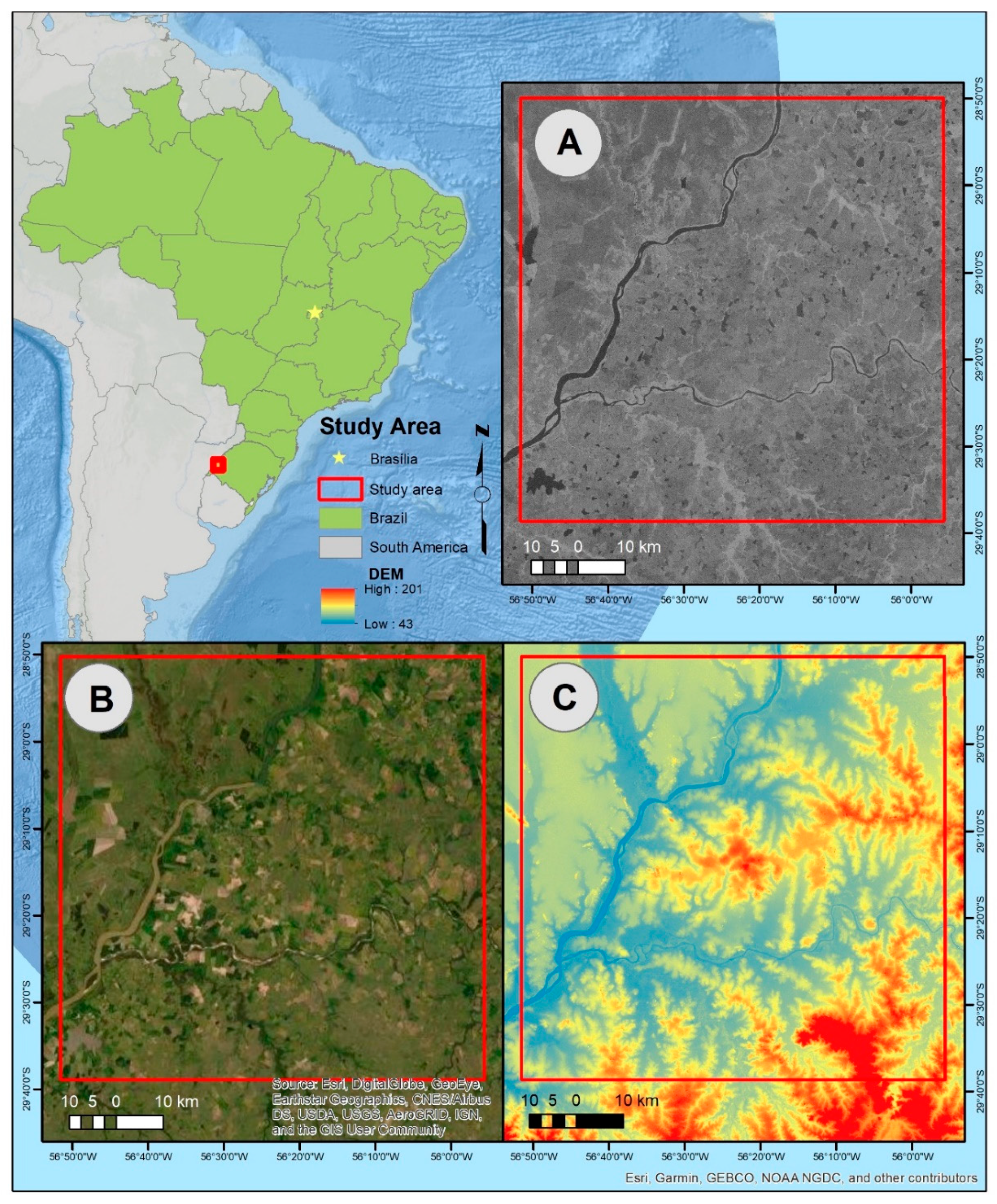
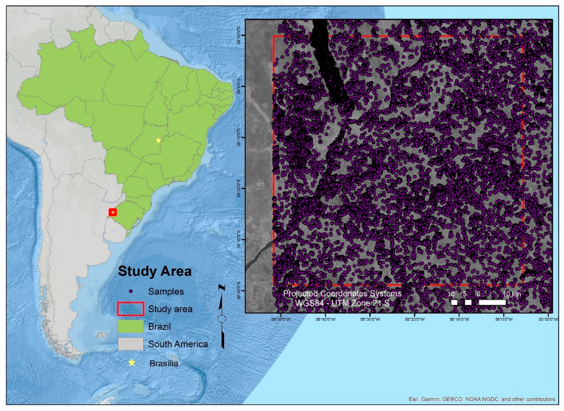
2. Study Area
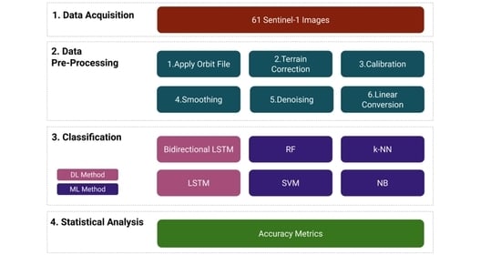
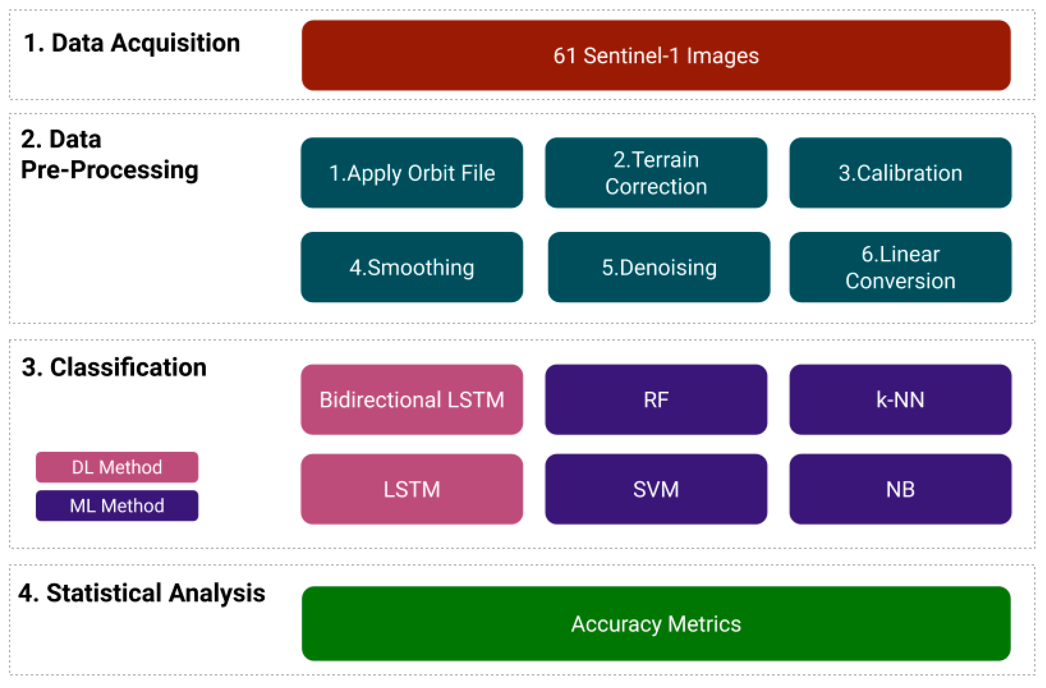
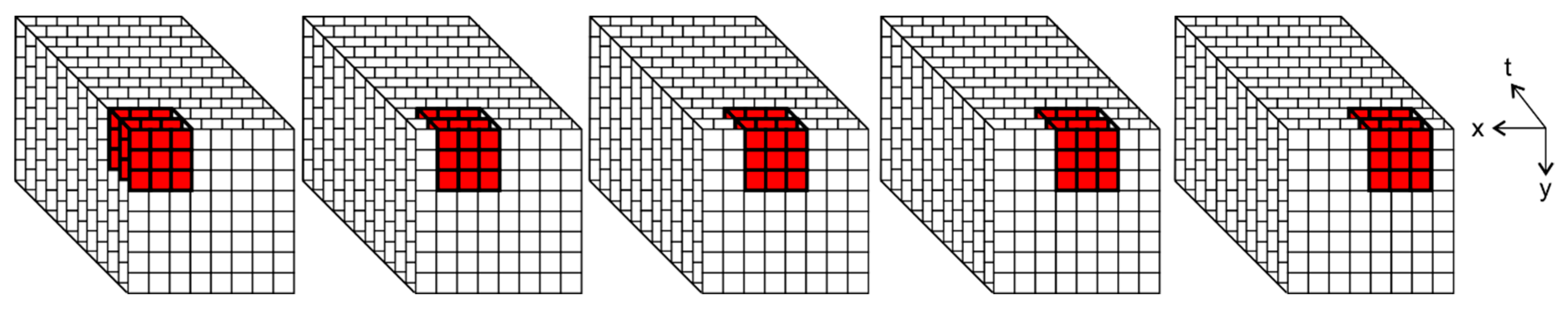
3. Materials and Methods
3.1. Dataset and Pre-Processing
3.2. SAR Image Denoising
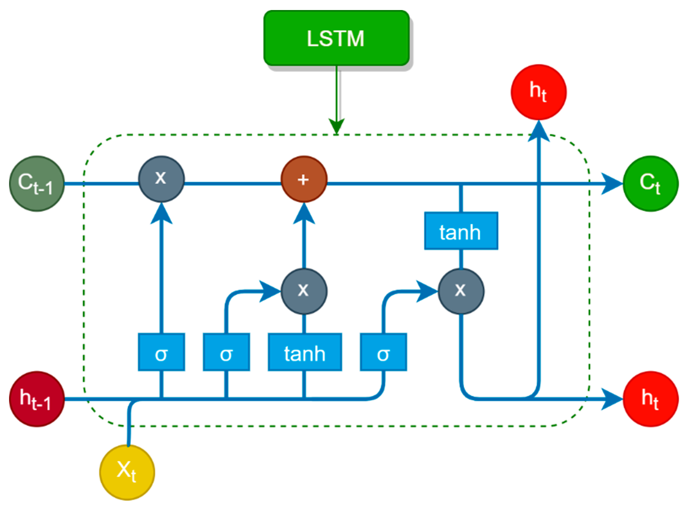
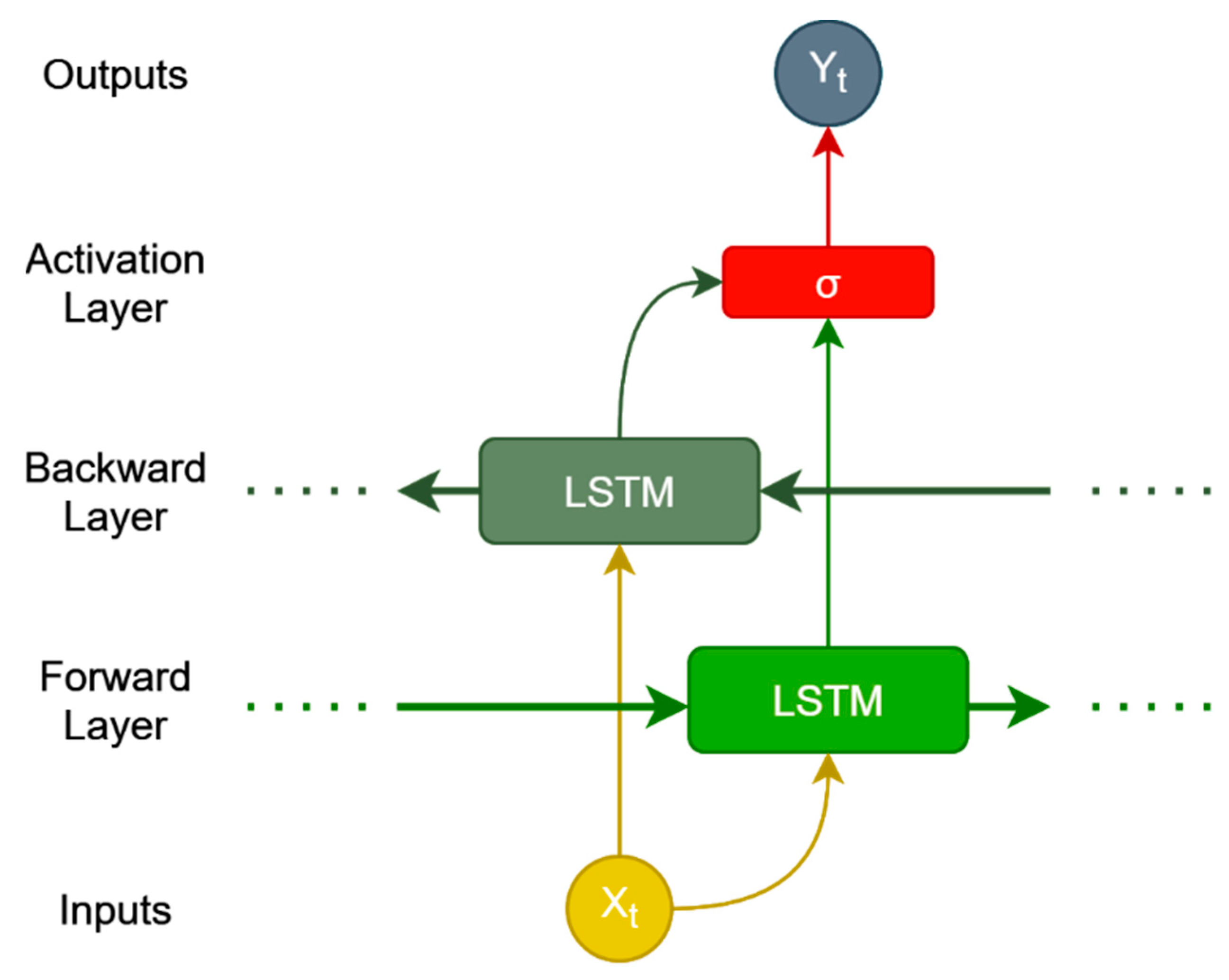
3.3. RNN and Traditional Machine Learning Models
3.4. Accuracy Assessment
4. Results
4.1. Image Denoising
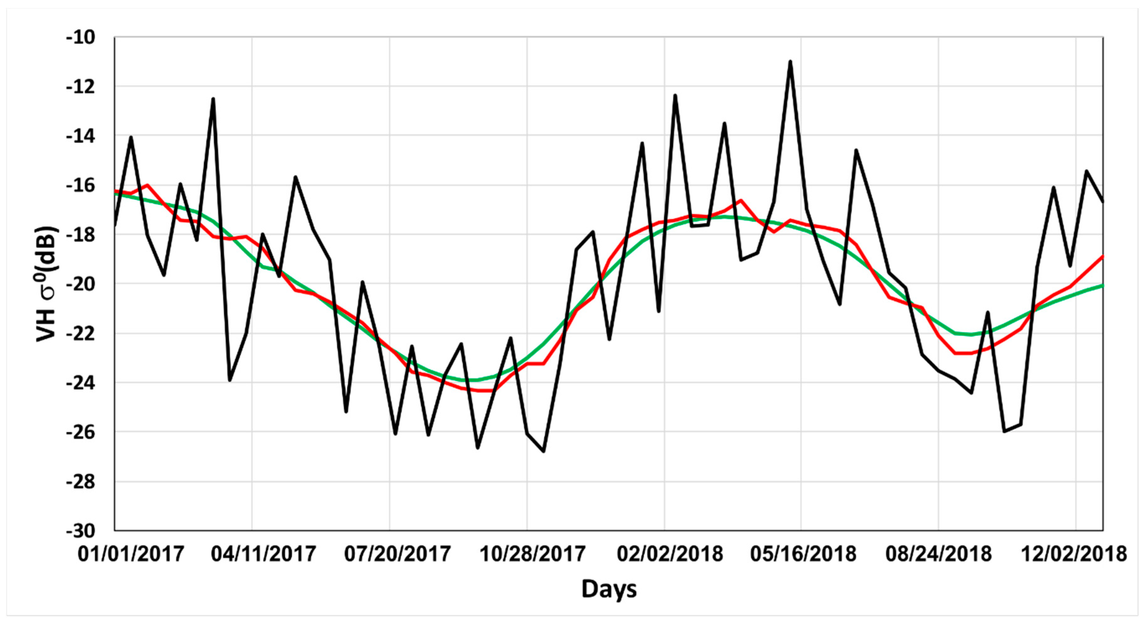
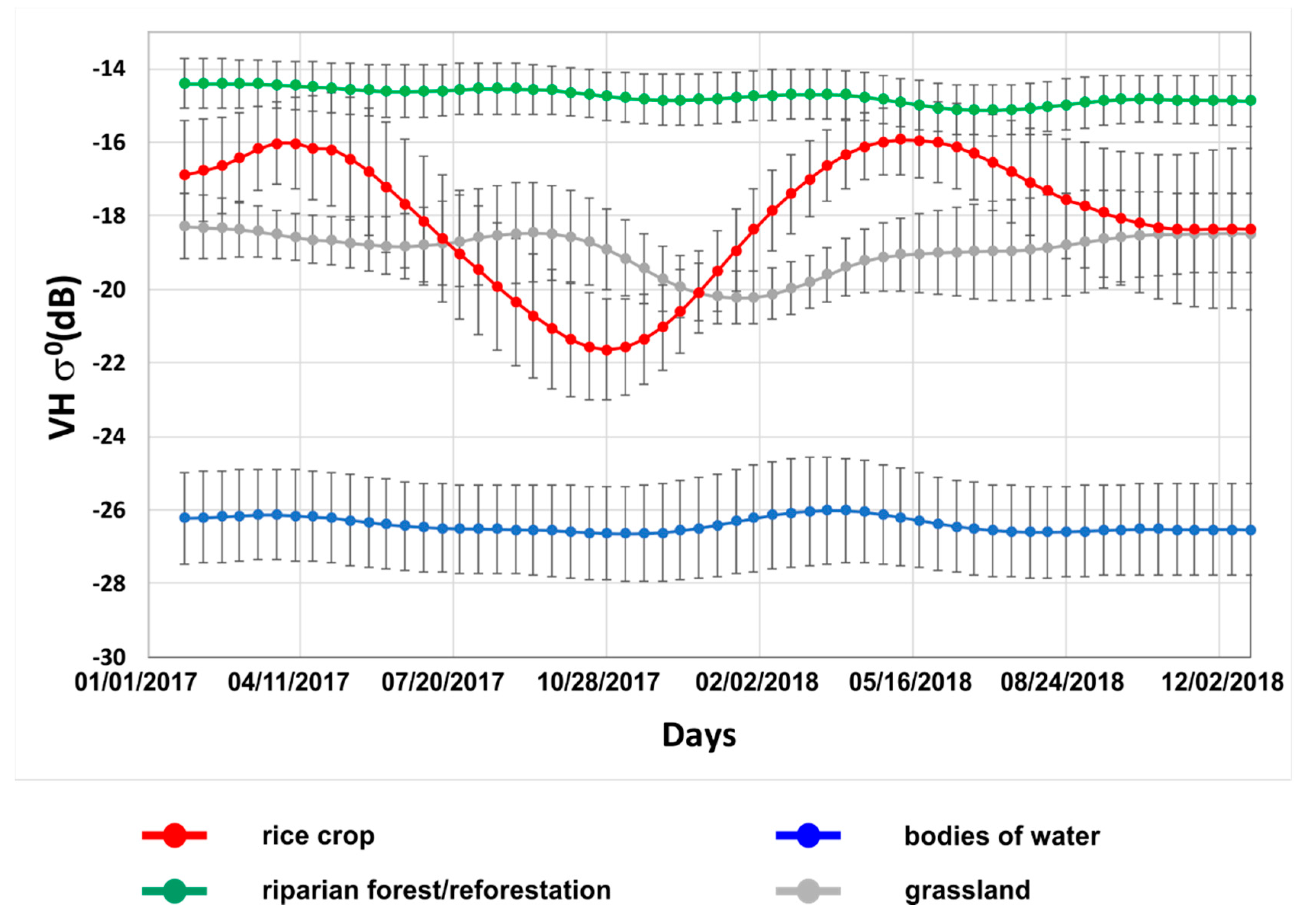
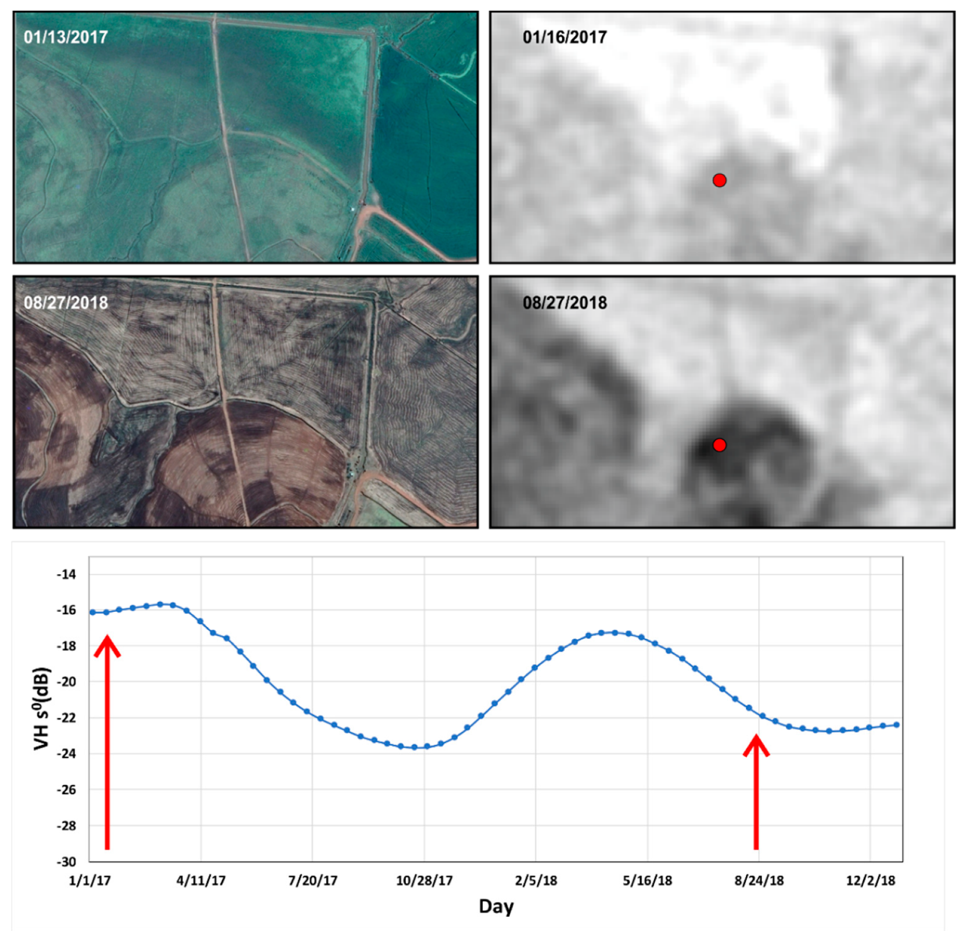
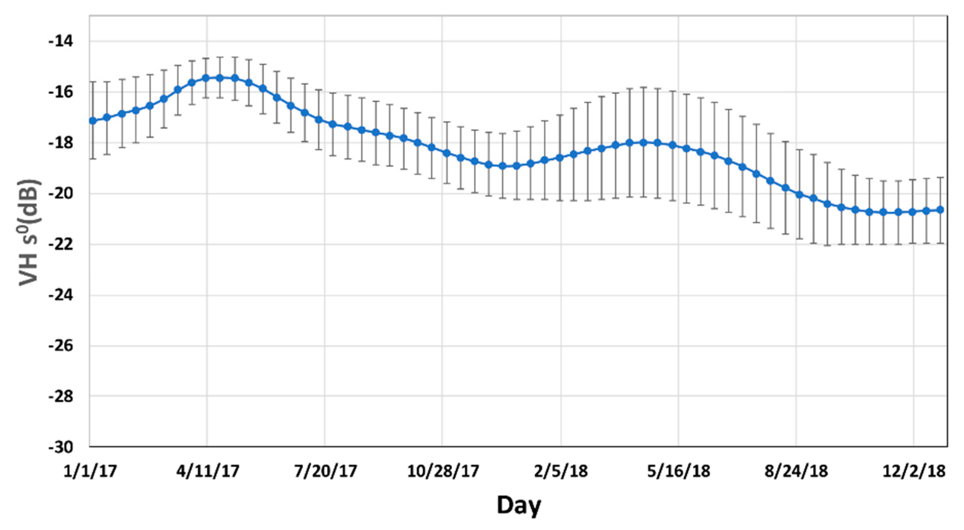
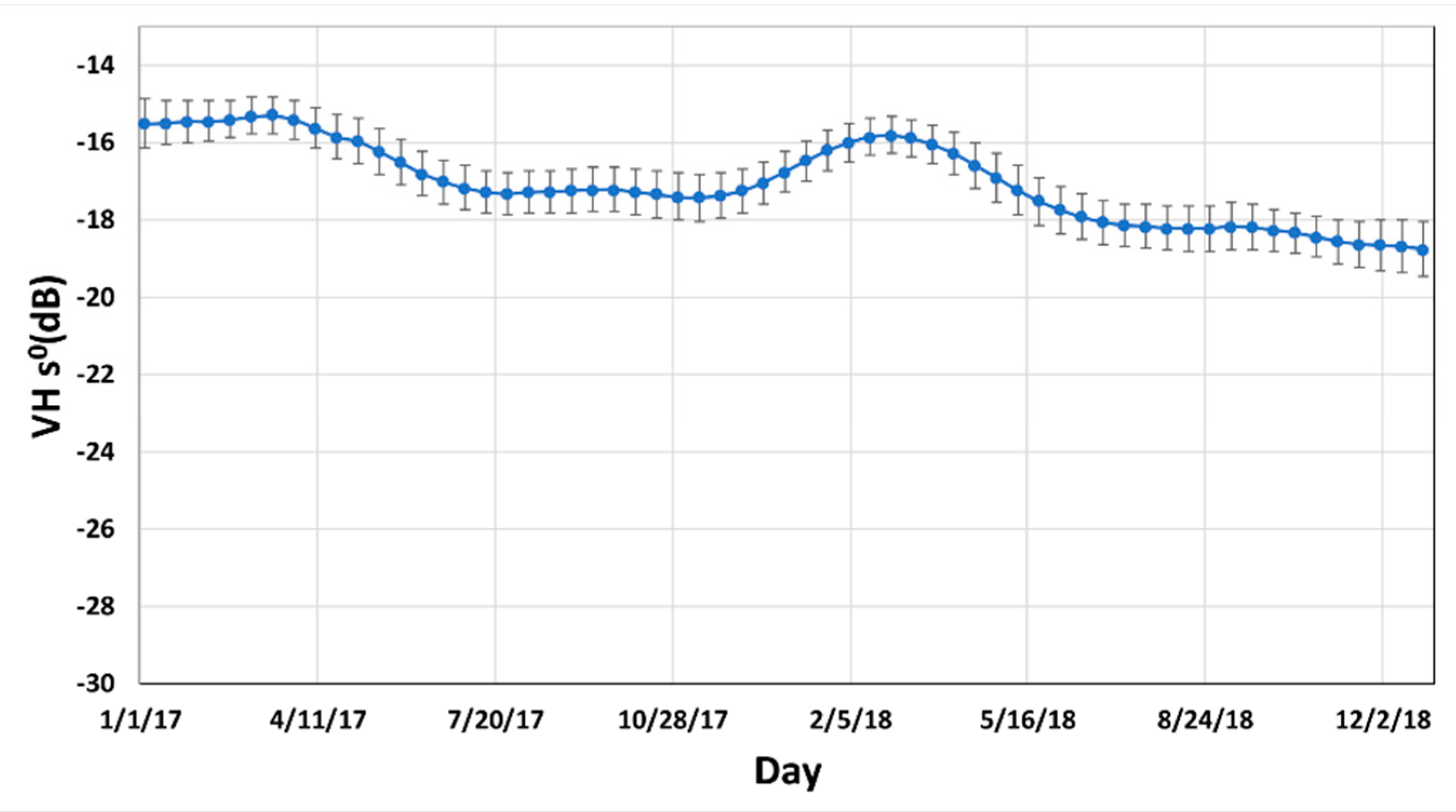
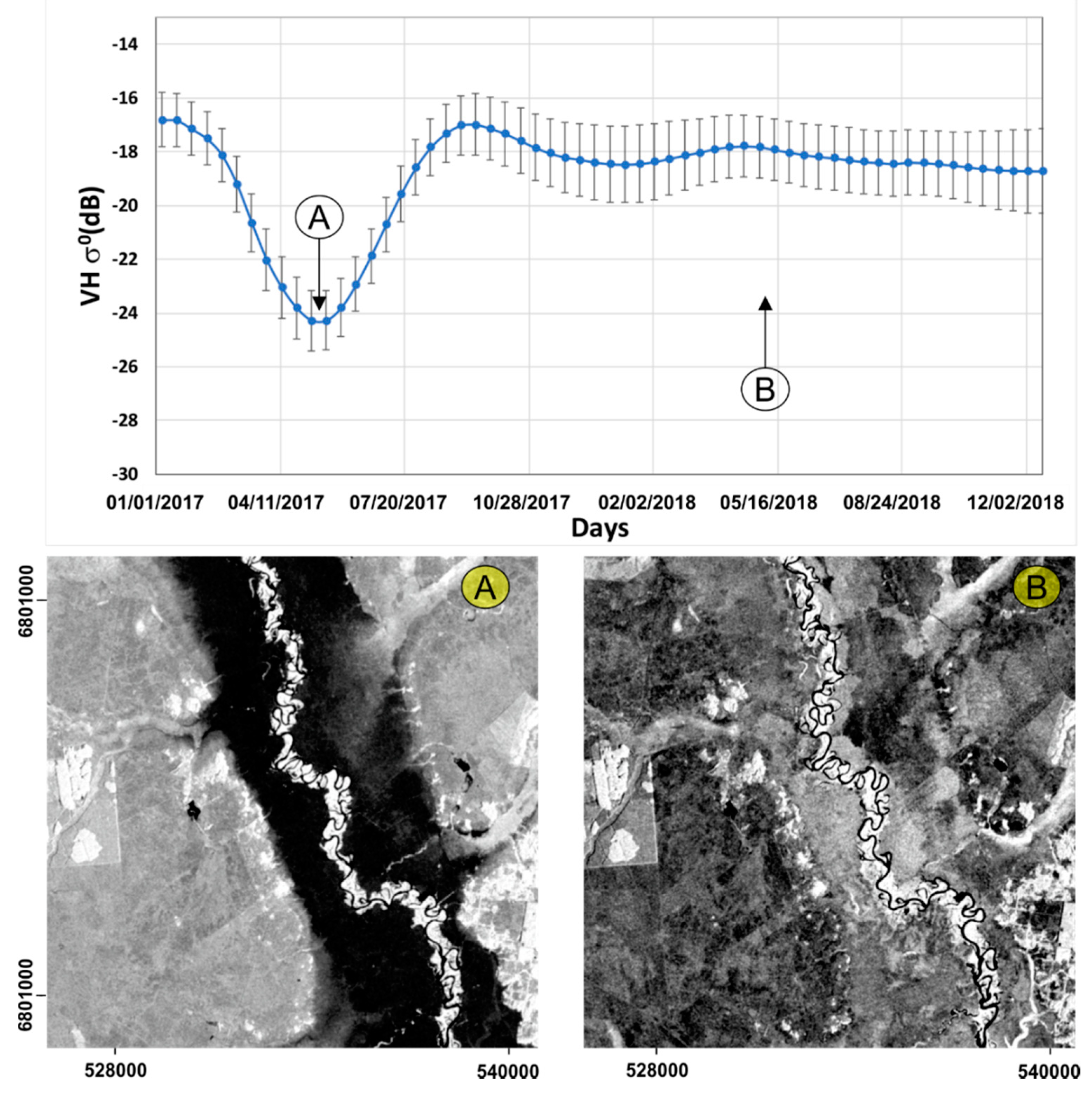
4.2. Temporal Backscattering Signatures
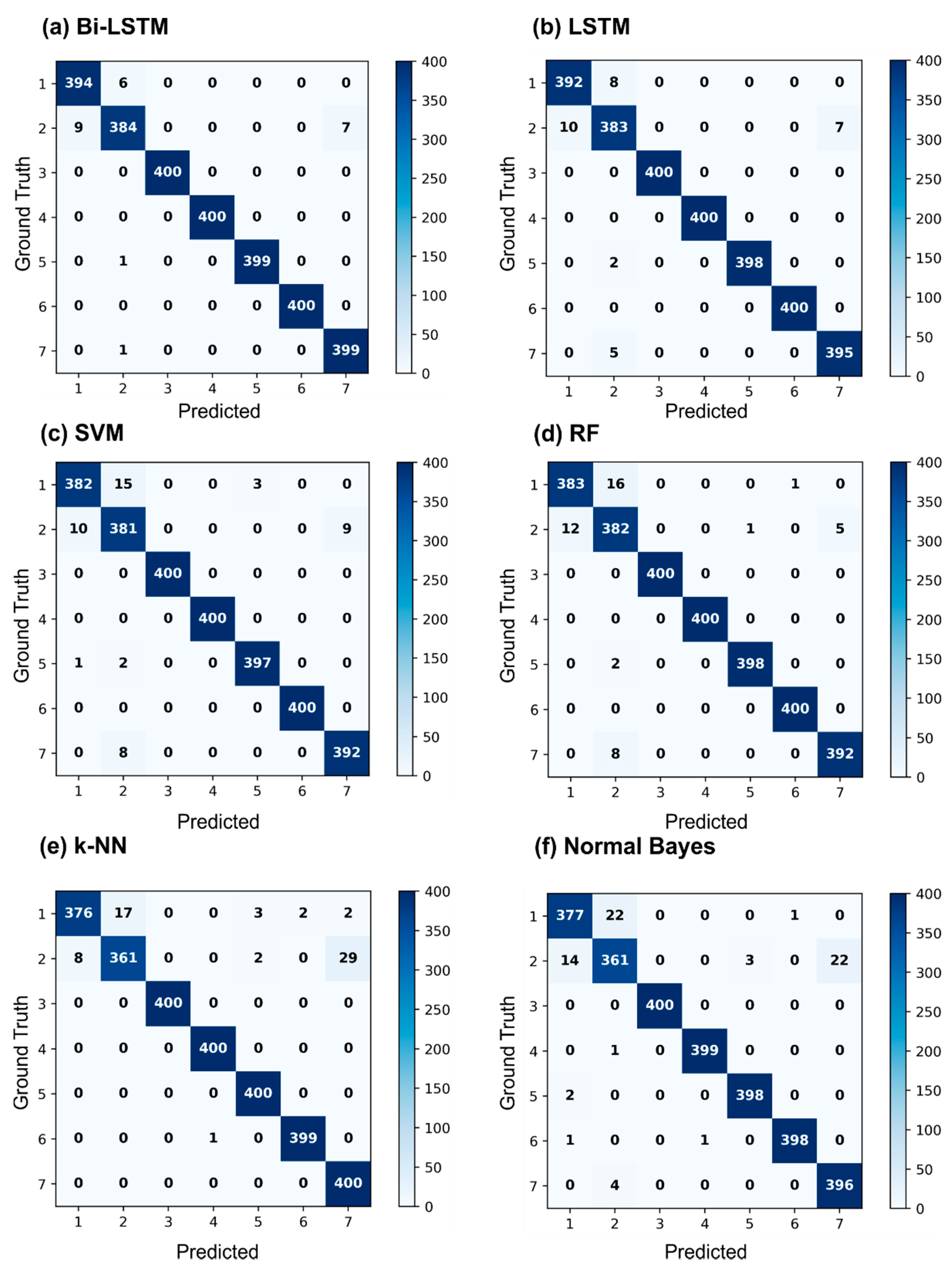
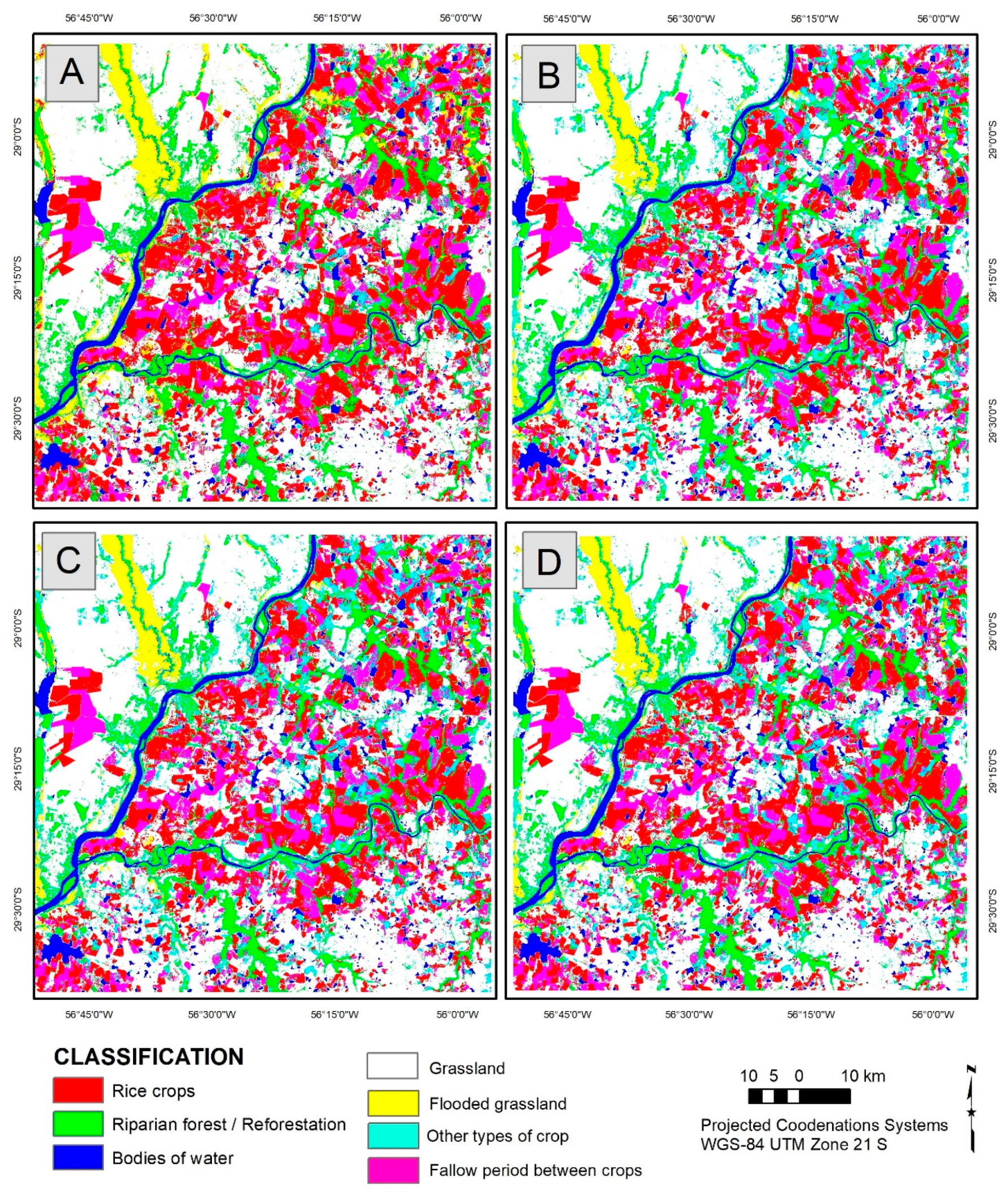
4.3. Comparison between RNN and Traditional Machine Learning Methods
5. Discussion
6. Conclusions
Author Contributions
Funding
Acknowledgments
Conflicts of Interest
References
- Laborte, A.G.; Gutierrez, M.A.; Balanza, J.G.; Saito, K.; Zwart, S.J.; Boschetti, M.; Murty, M.V.R.; Villano, L.; Aunario, J.K.; Reinke, R.; et al. RiceAtlas, a spatial database of global rice calendars and production. Sci. Data 2017, 4, 1–10. [Google Scholar] [CrossRef] [PubMed]
- Frolking, S.; Qiu, J.; Boles, S.; Xiao, X.; Liu, J.; Zhuang, Y.; Li, C.; Qin, X. Combining remote sensing and ground census data to develop new maps of the distribution of rice agriculture in China. Glob. Biogeochem. Cycles 2002, 16, 38-1–38-10. [Google Scholar] [CrossRef] [Green Version]
- Jin, X.; Kumar, L.; Li, Z.; Feng, H.; Xu, X.; Yang, G.; Wang, J. A review of data assimilation of remote sensing and crop models. Eur. J. Agron. 2018, 92, 141–152. [Google Scholar] [CrossRef]
- Steele-Dunne, S.C.; McNairn, H.; Monsivais-Huertero, A.; Judge, J.; Liu, P.-W.; Papathanassiou, K. Radar Remote Sensing of Agricultural Canopies: A Review. IEEE J. Sel. Top. Appl. Earth Obs. Remote Sens. 2017, 10, 2249–2273. [Google Scholar] [CrossRef] [Green Version]
- Vibhute, A.D.; Gawali, B.W. Analysis and Modeling of Agricultural Land use using Remote Sensing and Geographic Information System: A Review. Int. J. Eng. Res. Appl. 2013, 3, 81–91. [Google Scholar]
- Dong, J.; Xiao, X. Evolution of regional to global paddy rice mapping methods: A review. ISPRS J. Photogramm. Remote Sens. 2016, 119, 214–227. [Google Scholar] [CrossRef] [Green Version]
- Kuenzer, C.; Knauer, K. Remote sensing of rice crop areas. Int. J. Remote Sens. 2013, 34, 2101–2139. [Google Scholar] [CrossRef]
- Mosleh, M.K.; Hassan, Q.K.; Chowdhury, E.H. Application of remote sensors in mapping rice area and forecasting its production: A review. Sensors 2015, 15, 769–791. [Google Scholar] [CrossRef] [Green Version]
- Fang, H. Rice crop area estimation of an administrative division in China using remote sensing data. Int. J. Remote Sens. 1998, 19, 3411–3419. [Google Scholar] [CrossRef]
- McCloy, K.R.; Smith, F.R.; Robinson, M.R. Monitoring rice areas using LANDSAT MSS data. Int. J. Remote Sens. 1987, 8, 741–749. [Google Scholar] [CrossRef]
- Turner, M.D.; Congalton, R.G. Classification of multi-temporal SPOT-XS satellite data for mapping rice fields on a West African floodplain. Int. J. Remote Sens. 1998, 19, 21–41. [Google Scholar] [CrossRef]
- Liew, S.C. Application of multitemporal ers-2 synthetic aperture radar in delineating rice cropping systems in the mekong river delta, vietnam. IEEE Trans. Geosci. Remote Sens. 1998, 36, 1412–1420. [Google Scholar] [CrossRef]
- Kurosu, T.; Fujita, M.; Chiba, K. The identification of rice fields using multi-temporal ers-1 c band sar data. Int. J. Remote Sens. 1997, 18, 2953–2965. [Google Scholar] [CrossRef]
- Panigrahy, S.; Chakraborty, M.; Sharma, S.A.; Kundu, N.; Ghose, S.C.; Pal, M. Early estimation of rice area using temporal ERS-1 synthetic aperture radar data a case study for the Howrah and Hughly districts of West Bengal, India. Int. J. Remote Sens. 1997, 18, 1827–1833. [Google Scholar] [CrossRef]
- Okamoto, K.; Kawashima, H. Estimation of rice-planted area in the tropical zone using a combination of optical and microwave satellite sensor data. Int. J. Remote Sens. 1999, 20, 1045–1048. [Google Scholar] [CrossRef]
- Diuk-Wasser, M.A.; Bagayoko, M.; Sogoba, N.; Dolo, G.; Touré, M.B.; Traore, S.F.; Taylor, C.E. Mapping rice field anopheline breeding habitats in Mali, West Africa, using Landsat ETM + sensor data. Int. J. Remote Sens. 2004, 25, 359–376. [Google Scholar] [CrossRef] [PubMed] [Green Version]
- Kontgis, C.; Schneider, A.; Ozdogan, M. Mapping rice paddy extent and intensification in the Vietnamese Mekong River Delta with dense time stacks of Landsat data. Remote Sens. Environ. 2015, 169, 255–269. [Google Scholar] [CrossRef]
- Nuarsa, I.W.; Nishio, F.; Hongo, C. Spectral Characteristics and Mapping of Rice Plants Using Multi-Temporal Landsat Data. J. Agric. Sci. 2011, 3, 54–67. [Google Scholar] [CrossRef] [Green Version]
- Huang, J.; Wang, X.; Li, X.; Tian, H.; Pan, Z. Remotely Sensed Rice Yield Prediction Using Multi-Temporal NDVI Data Derived from NOAA’s-AVHRR. PLoS ONE 2013, 8, e0070816. [Google Scholar] [CrossRef]
- Salam, M.A.; Rahman, H. Application of Remote Sensing and Geographic Information System (GIS) Techniques for Monitoring of Boro Rice Area Expansion in Bangladesh. Asian J. Geoinform. 2014, 14, 11–17. [Google Scholar]
- Singh, R.P.; Oza, S.R.; Pandya, M.R. Observing long-term changes in rice phenology using NOAA-AVHRR and DMSP-SSM/I satellite sensor measurements in Punjab, India. Curr. Sci. 2006, 91, 1217–1221. [Google Scholar]
- Kamthonkiat, D.; Honda, K.; Turral, H.; Tripathi, N.K.; Wuwongse, V. Discrimination of irrigated and rainfed rice in a tropical agricultural system using SPOT VEGETATION NDVI and rainfall data. Int. J. Remote Sens. 2005, 26, 2527–2547. [Google Scholar] [CrossRef]
- Wang, L.; Zhang, F.C.; Jing, Y.S.; Jiang, X.D.; Yang, S.B.; Han, X.M. Multi-temporal detection of rice phenological stages using canopy stagespectrum. Rice Sci. 2014, 21, 108–115. [Google Scholar] [CrossRef]
- Nguyen, T.T.H.; de Bie, C.A.J.M.; Ali, A.; Smaling, E.M.A.; Chu, T.H. Mapping the irrigated rice cropping patterns of the Mekong delta, Vietnam, through hyper-temporal spot NDVI image analysis. Int. J. Remote Sens. 2012, 33, 415–434. [Google Scholar] [CrossRef]
- Gumma, M.K.; Nelson, A.; Thenkabail, P.S.; Singh, A.N. Mapping rice areas of South Asia using MODIS multitemporal data. J. Appl. Remote Sens. 2011, 5, 053547. [Google Scholar] [CrossRef] [Green Version]
- Gumma, M.K.; Gauchan, D.; Nelson, A.; Pandey, S.; Rala, A. Temporal changes in rice-growing area and their impact on livelihood over a decade: A case study of Nepal. Agric. Ecosyst. Environ. 2011, 142, 382–392. [Google Scholar] [CrossRef]
- Nuarsa, I.W.; Nishio, F.; Hongo, C.; Mahardika, I.G. Using variance analysis of multitemporal MODIS images for rice field mapping in Bali Province, Indonesia. Int. J. Remote Sens. 2012, 33, 5402–5417. [Google Scholar] [CrossRef]
- Peng, D.; Huete, A.R.; Huang, J.; Wang, F.; Sun, H. Detection and estimation of mixed paddy rice cropping patterns with MODIS data. Int. J. Appl. Earth Obs. Geoinf. 2011, 13, 13–23. [Google Scholar] [CrossRef]
- Xiao, X.; Boles, S.; Liu, J.; Zhuang, D.; Frolking, S.; Li, C.; Salas, W.; Moore, B. Mapping paddy rice agriculture in southern China using multi-temporal MODIS images. Remote Sens. Environ. 2005, 95, 480–492. [Google Scholar] [CrossRef]
- Xiao, X.; Boles, S.; Frolking, S.; Li, C.; Babu, J.Y.; Salas, W.; Moore, B. Mapping paddy rice agriculture in South and Southeast Asia using multi-temporal MODIS images. Remote Sens. Environ. 2006, 100, 95–113. [Google Scholar] [CrossRef]
- Lopez-Sanchez, J.M.; Ballester-Berman, J.D.; Hajnsek, I.; Hajnsek, I. First Results of Rice Monitoring Practices in Spain by Means of Time Series of TerraSAR-X Dual-Pol Images. IEEE J. Sel. Top. Appl. Earth Obs. Remote Sens. 2011, 4, 412–422. [Google Scholar] [CrossRef]
- Koppe, W.; Gnyp, M.L.; Hütt, C.; Yao, Y.; Miao, Y.; Chen, X.; Bareth, G. Rice monitoring with multi-temporal and dual-polarimetric terrasar-X data. Int. J. Appl. Earth Obs. Geoinf. 2012, 21, 568–576. [Google Scholar] [CrossRef]
- Nelson, A.; Setiyono, T.; Rala, A.B.; Quicho, E.D.; Raviz, J.V.; Abonete, P.J.; Maunahan, A.A.; Garcia, C.A.; Bhatti, H.Z.M.; Villano, L.S.; et al. Towards an operational SAR-based rice monitoring system in Asia: Examples from 13 demonstration sites across Asia in the RIICE project. Remote Sens. 2014, 6, 10773–10812. [Google Scholar] [CrossRef] [Green Version]
- Pei, Z.; Zhang, S.; Guo, L.; Mc Nairn, H.; Shang, J.; Jiao, X. Rice identification and change detection using TerraSAR-X data. Can. J. Remote Sens. 2011, 37, 151–156. [Google Scholar] [CrossRef]
- Asilo, S.; de Bie, K.; Skidmore, A.; Nelson, A.; Barbieri, M.; Maunahan, A. Complementarity of two rice mapping approaches: Characterizing strata mapped by hypertemporal MODIS and rice paddy identification using multitemporal SAR. Remote Sens. 2014, 6, 12789–12814. [Google Scholar] [CrossRef] [Green Version]
- Busetto, L.; Casteleyn, S.; Granell, C.; Pepe, M.; Barbieri, M.; Campos-Taberner, M.; Casa, R.; Collivignarelli, F.; Confalonieri, R.; Crema, A.; et al. Downstream Services for Rice Crop Monitoring in Europe: From Regional to Local Scale. IEEE J. Sel. Top. Appl. Earth Obs. Remote Sens. 2017, 10, 5423–5441. [Google Scholar] [CrossRef] [Green Version]
- Corcione, V.; Nunziata, F.; Mascolo, L.; Migliaccio, M. A study of the use of COSMO-SkyMed SAR PingPong polarimetric mode for rice growth monitoring. Int. J. Remote Sens. 2016, 37, 633–647. [Google Scholar] [CrossRef]
- Phan, H.; Le Toan, T.; Bouvet, A.; Nguyen, L.D.; Duy, T.P.; Zribi, M. Mapping of rice varieties and sowing date using X-band SAR data. Sensors 2018, 18, 316. [Google Scholar] [CrossRef] [PubMed] [Green Version]
- Chakraborty, M.; Panigrahy, S.; Sharma, S.A. Discrimination of rice crop grown under different cultural practices using temporal ERS-1 synthetic aperture radar data. ISPRS J. Photogramm. Remote Sens. 1997, 52, 183–191. [Google Scholar] [CrossRef]
- Jia, M.; Tong, L.; Chen, Y.; Wang, Y.; Zhang, Y. Rice biomass retrieval from multitemporal ground-based scatterometer data and RADARSAT-2 images using neural networks. J. Appl. Remote Sens. 2013, 7, 073509. [Google Scholar] [CrossRef]
- McNairn, H.; Brisco, B. The application of C-band polarimetric SAR for agriculture: A review. Can. J. Remote Sens. 2004, 30, 525–542. [Google Scholar] [CrossRef]
- Chakraborty, M.; Manjunath, K.R.; Panigrahy, S.; Kundu, N.; Parihar, J.S. Rice crop parameter retrieval using multi-temporal, multi-incidence angle Radarsat SAR data. ISPRS J. Photogramm. Remote Sens. 2005, 59, 310–322. [Google Scholar] [CrossRef]
- Choudhury, I.; Chakraborty, M. SAR sig nature investigation of rice crop using RADARSAT data. Int. J. Remote Sens. 2006, 27, 519–534. [Google Scholar] [CrossRef]
- He, Z.; Li, S.; Wang, Y.; Dai, L.; Lin, S. Monitoring rice phenology based on backscattering characteristics of multi-temporal RADARSAT-2 datasets. Remote Sens. 2018, 10, 340. [Google Scholar] [CrossRef] [Green Version]
- Shao, Y.; Fan, X.; Liu, H.; Xiao, J.; Ross, S.; Brisco, B.; Brown, R.; Staples, G. Rice monitoring and production estimation using multitemporal RADARSAT. Remote Sens. Environ. 2001, 76, 310–325. [Google Scholar] [CrossRef]
- Wu, F.; Wang, C.; Zhang, H.; Zhang, B.; Tang, Y. Rice crop monitoring in South China with RADARSAT-2 quad-polarization SAR data. IEEE Geosci. Remote Sens. Lett. 2011, 8, 196–200. [Google Scholar] [CrossRef]
- Yonezawa, C.; Negishi, M.; Azuma, K.; Watanabe, M.; Ishitsuka, N.; Ogawa, S.; Saito, G. Growth monitoring and classification of rice fields using multitemporal RADARSAT-2 full-polarimetric data. Int. J. Remote Sens. 2012, 33, 5696–5711. [Google Scholar] [CrossRef]
- Bouvet, A.; Le Toan, T.; Lam-Dao, N. Monitoring of the rice cropping system in the Mekong Delta using ENVISAT/ASAR dual polarization data. IEEE Trans. Geosci. Remote Sens. 2009, 47, 517–526. [Google Scholar] [CrossRef] [Green Version]
- Bouvet, A.; Le Toan, T. Use of ENVISAT/ASAR wide-swath data for timely rice fields mapping in the Mekong River Delta. Remote Sens. Environ. 2011, 115, 1090–1101. [Google Scholar] [CrossRef] [Green Version]
- Chen, J.; Lin, H.; Pei, Z. Application of ENVISAT ASAR data in mapping rice crop growth in southern China. IEEE Geosci. Remote Sens. Lett. 2007, 4, 431–435. [Google Scholar] [CrossRef]
- Nguyen, D.B.; Clauss, K.; Cao, S.; Naeimi, V.; Kuenzer, C.; Wagner, W. Mapping Rice Seasonality in the Mekong Delta with multi-year envisat ASAR WSM Data. Remote Sens. 2015, 7, 15868–15893. [Google Scholar] [CrossRef] [Green Version]
- Yang, S.; Shen, S.; Li, B.; Le Toan, T.; He, W. Rice mapping and monitoring using ENVISAT ASAR data. IEEE Geosci. Remote Sens. Lett. 2008, 5, 108–112. [Google Scholar] [CrossRef]
- Wang, C.; Wu, J.; Zhang, Y.; Pan, G.; Qi, J.; Salas, W.A. Characterizing L-band scattering of paddy rice in southeast china with radiative transfer model and multitemporal ALOS/PALSAR imagery. IEEE Trans. Geosci. Remote Sens. 2009, 47, 988–998. [Google Scholar] [CrossRef]
- Zhang, Y.; Wang, C.; Wu, J.; Qi, J.; Salas, W.A. Mapping paddy rice with multitemporal ALOS/PALSAR imagery in southeast China. Int. J. Remote Sens. 2009, 30, 6301–6315. [Google Scholar] [CrossRef]
- Zhang, Y.; Wang, C.; Zhang, Q. Identifying paddy fields with dual-polarization ALOS/PALSAR data. Can. J. Remote Sens. 2011, 37, 103–111. [Google Scholar] [CrossRef]
- Singha, M.; Dong, J.; Zhang, G.; Xiao, X. High resolution paddy rice maps in cloud-prone Bangladesh and Northeast India using Sentinel-1 data. Sci. Data 2019, 6, 1–10. [Google Scholar] [CrossRef]
- Clauss, K.; Ottinger, M.; Kuenzer, C. Mapping rice areas with Sentinel-1 time series and superpixel segmentation. Int. J. Remote Sens. 2018, 39, 1399–1420. [Google Scholar] [CrossRef] [Green Version]
- Bazzi, H.; Baghdadi, N.; Ienco, D.; El Hajj, M.; Zribi, M.; Belhouchette, H.; Escorihuela, M.J.; Demarez, V. Mapping irrigated areas using Sentinel-1 time series in Catalonia, Spain. Remote Sens. 2019, 11, 1836. [Google Scholar] [CrossRef] [Green Version]
- Mandal, D.; Kumar, V.; Bhattacharya, A.; Rao, Y.S.; Siqueira, P.; Bera, S. Sen4Rice: A processing chain for differentiating early and late transplanted rice using time-series sentinel-1 SAR data with google earth engine. IEEE Geosci. Remote Sens. Lett. 2018, 15, 1947–1951. [Google Scholar] [CrossRef]
- Inoue, S.; Ito, A.; Yonezawa, C. Mapping Paddy fields in Japan by using a Sentinel-1 SAR time series supplemented by Sentinel-2 images on Google Earth Engine. Remote Sens. 2020, 12, 1622. [Google Scholar] [CrossRef]
- Clauss, K.; Ottinger, M.; Leinenkugel, P.; Kuenzer, C. Estimating rice production in the Mekong Delta, Vietnam, utilizing time series of Sentinel-1 SAR data. Int. J. Appl. Earth Obs. Geoinf. 2018, 73, 574–585. [Google Scholar] [CrossRef]
- Minh, H.V.T.; Avtar, R.; Mohan, G.; Misra, P.; Kurasaki, M. Monitoring and mapping of rice cropping pattern in flooding area in the Vietnamese Mekong delta using Sentinel-1A data: A case of an Giang province. ISPRS Int. J. Geo-Inf. 2019, 8, 211. [Google Scholar] [CrossRef] [Green Version]
- Nguyen, D.B.; Gruber, A.; Wagner, W. Mapping rice extent and cropping scheme in the Mekong Delta using Sentinel-1A data. Remote Sens. Lett. 2016, 7, 1209–1218. [Google Scholar] [CrossRef]
- Son, N.T.; Chen, C.F.; Chen, C.R.; Minh, V.Q. Assessment of Sentinel-1A data for rice crop classification using random forests and support vector machines. Geocarto Int. 2018, 33, 587–601. [Google Scholar] [CrossRef]
- Onojeghuo, A.O.; Blackburn, G.A.; Wang, Q.; Atkinson, P.M.; Kindred, D.; Miao, Y. Mapping paddy rice fields by applying machine learning algorithms to multi-temporal sentinel-1A and landsat data. Int. J. Remote Sens. 2018, 39, 1042–1067. [Google Scholar] [CrossRef] [Green Version]
- Tian, H.; Wu, M.; Wang, L.; Niu, Z. Mapping early, middle and late rice extent using Sentinel-1A and Landsat-8 data in the poyang lake plain, China. Sensors 2018, 18, 185. [Google Scholar] [CrossRef] [Green Version]
- Torbick, N.; Chowdhury, D.; Salas, W.; Qi, J. Monitoring Rice Agriculture across Myanmar Using Time Series Sentinel-1 Assisted by Landsat-8 and PALSAR-2. Remote Sens. 2017, 9, 119. [Google Scholar] [CrossRef] [Green Version]
- Zhang, X.; Wu, B.; Ponce-Campos, G.E.; Zhang, M.; Chang, S.; Tian, F. Mapping up-to-date paddy rice extent at 10 M resolution in China through the integration of optical and synthetic aperture radar images. Remote Sens. 2018, 10, 1200. [Google Scholar] [CrossRef] [Green Version]
- Guo, Y.; Liu, Y.; Oerlemans, A.; Lao, S.; Wu, S.; Lew, M.S. Deep learning for visual understanding: A review. Neurocomputing 2016, 187, 27–48. [Google Scholar] [CrossRef]
- Liu, L.; Ouyang, W.; Wang, X.; Fieguth, P.; Chen, J.; Liu, X.; Pietikäinen, M. Deep Learning for Generic Object Detection: A Survey. Int. J. Comput. Vis. 2020, 128, 261–318. [Google Scholar] [CrossRef] [Green Version]
- Voulodimos, A.; Doulamis, N.; Doulamis, A.; Protopapadakis, E. Deep Learning for Computer Vision: A Brief Review. Comput. Intell. Neurosci. 2018, 2018. [Google Scholar] [CrossRef] [PubMed]
- Ma, L.; Liu, Y.; Zhang, X.; Ye, Y.; Yin, G.; Johnson, B.A. Deep learning in remote sensing applications: A meta-analysis and review. ISPRS J. Photogramm. Remote Sens. 2019, 152, 166–177. [Google Scholar] [CrossRef]
- Yu, X.; Wu, X.; Luo, C.; Ren, P. Deep learning in remote sensing scene classification: A data augmentation enhanced convolutional neural network framework. GISci. Remote Sens. 2017, 54, 741–758. [Google Scholar] [CrossRef] [Green Version]
- Zhu, X.X.; Tuia, D.; Mou, L.; Xia, G.; Zhang, L.; Xu, F.; Fraundorfer, F. Deep Learning in Remote Sensing: A Comprehensive Review and List of Resources. IEEE Geosci. Remote Sens. Mag. 2017, 5, 8–36. [Google Scholar] [CrossRef] [Green Version]
- Mou, L.; Bruzzone, L.; Zhu, X.X. Learning spectral-spatialoral features via a recurrent convolutional neural network for change detection in multispectral imagery. IEEE Trans. Geosci. Remote Sens. 2019, 57, 924–935. [Google Scholar] [CrossRef] [Green Version]
- Hochreiter, S.; Schmidhuber, J. Long Short-Term Memory. Neural Comput. 1997, 9, 1735–1780. [Google Scholar] [CrossRef] [PubMed]
- Lyu, H.; Lu, H.; Mou, L. Learning a transferable change rule from a recurrent neural network for land cover change detection. Remote Sens. 2016, 8, 506. [Google Scholar] [CrossRef] [Green Version]
- He, T.; Xie, C.; Liu, Q.; Guan, S.; Liu, G. Evaluation and comparison of random forest and A-LSTM networks for large-scale winter wheat identification. Remote Sens. 2019, 11, 1665. [Google Scholar] [CrossRef] [Green Version]
- Rußwurm, M.; Körner, M. Multi-temporal land cover classification with sequential recurrent encoders. ISPRS Int. J. Geo-Inf. 2018, 7, 129. [Google Scholar] [CrossRef] [Green Version]
- Sun, Z.; Di, L.; Fang, H. Using long short-term memory recurrent neural network in land cover classification on Landsat and Cropland data layer time series. Int. J. Remote Sens. 2019, 40, 593–614. [Google Scholar] [CrossRef]
- Teimouri, N.; Dyrmann, M.; Jørgensen, R.N. A novel spatio-temporal FCN-LSTM network for recognizing various crop types using multi-temporal radar images. Remote Sens. 2019, 11, 893. [Google Scholar] [CrossRef] [Green Version]
- Zhou, Y.; Luo, J.; Feng, L.; Yang, Y.; Chen, Y.; Wu, W. Long-short-term-memory-based crop classification using high-resolution optical images and multi-temporal SAR data. GISci. Remote Sens. 2019, 56, 1170–1191. [Google Scholar] [CrossRef]
- Ienco, D.; Gaetano, R.; Dupaquier, C.; Maurel, P. Land Cover Classification via Multitemporal Spatial Data by Deep Recurrent Neural Networks. IEEE Geosci. Remote Sens. Lett. 2017, 14, 1685–1689. [Google Scholar] [CrossRef] [Green Version]
- Wang, H.; Zhao, X.; Zhang, X.; Wu, D.; Du, X. Long time series land cover classification in China from 1982 to 2015 based on Bi-LSTM deep learning. Remote Sens. 2019, 11, 1639. [Google Scholar] [CrossRef] [Green Version]
- Reddy, D.S.; Prasad, P.R.C. Prediction of vegetation dynamics using NDVI time series data and LSTM. Model. Earth Syst. Environ. 2018, 4, 409–419. [Google Scholar] [CrossRef]
- USDA FAS—United States Department of Agriculture—Foreign Agricultural Service. World Agricultural Production. Available online: https://apps.fas.usda.gov/psdonline/circulars/production.pdf (accessed on 19 May 2020).
- Companhia Nacional de Abastecimento. Acompanhamento da Safra Brasileira: Grãos, Quarto Levantamento—Janeiro/2020; Companhia Nacional de Abastecimento: Brasilia, Brazil, 2020; Volume 7, p. 104. [Google Scholar]
- IBGE—Instituto Brasileiro de Geografia e Estatística. Cidades@. Available online: https://cidades.ibge.gov.br/ (accessed on 25 May 2020).
- IBGE—Instituto Brasileiro de Geografia e Estatística. Produção Agrícola Municipal—PAM. Available online: https://www.ibge.gov.br/estatisticas/economicas/agricultura-e-pecuaria/9117-producao-agricola-municipal-culturas-temporarias-e-permanentes.html?=&t=o-que-e (accessed on 25 May 2020).
- Robaina, L.E.D.S.; Trentin, R.; Laurent, F. Compartimentação do Estado do Rio Grande do Sul, Brasil, através do Uso de Geomorphons Obtidos em Classificação Topográfica Automatizada. Rev. Bras. Geomorfol. 2016, 17. [Google Scholar] [CrossRef] [Green Version]
- Trentin, R.; Robaina, L.E.D.S. Study of the landforms of the ibicuí river basin with use of topographic position index. Rev. Bras. Geomorfol. 2018, 19. [Google Scholar] [CrossRef] [Green Version]
- Martins, L.C.; Wildner, W.; Hartmann, L.A. Estratigrafia dos derrames da Província Vulcânica Paraná na região oeste do Rio Grande do Sul, Brasil, com base em sondagem, perfilagem gamaespectrométrica e geologia de campo. Pesqui. Geociências 2011, 38, 15. [Google Scholar] [CrossRef] [Green Version]
- Moreira, A.; Bremm, C.; Fontana, D.C.; Kuplich, T.M. Seasonal dynamics of vegetation indices as a criterion for grouping grassland typologies. Sci. Agric. 2019, 76, 24–32. [Google Scholar] [CrossRef]
- Maltchik, L. Three new wetlands inventories in Brazil. Interciencia 2003, 28, 421–423. [Google Scholar]
- Guadagnin, D.L.; Peter, A.S.; Rolon, A.S.; Stenert, C.; Maltchik, L. Does Non-Intentional Flooding of Rice Fields After Cultivation Contribute to Waterbird Conservation in Southern Brazil? Waterbirds 2012, 35, 371–380. [Google Scholar] [CrossRef]
- Machado, I.F.; Maltchik, L. Can management practices in rice fields contribute to amphibian conservation in southern Brazilian wetlands? Aquat. Conserv. Mar. Freshw. Ecosyst. 2010, 20, 39–46. [Google Scholar] [CrossRef]
- Rolon, A.S.; Maltchik, L. Does flooding of rice fields after cultivation contribute to wetland plant conservation in southern Brazil? Appl. Veg. Sci. 2010, 13, 26–35. [Google Scholar] [CrossRef]
- Stenert, C.; Bacca, R.C.; Maltchik, L.; Rocha, O. Can hydrologic management practices of rice fields contribute to macroinvertebrate conservation in southern brazil wetlands? Hydrobiologia 2009, 635, 339–350. [Google Scholar] [CrossRef]
- Maltchik, L.; Stenert, C.; Batzer, D.P. Can rice field management practices contribute to the conservation of species from natural wetlands? Lessons from Brazil. Basic Appl. Ecol. 2017, 18, 50–56. [Google Scholar] [CrossRef]
- Torres, R.; Snoeij, P.; Geudtner, D.; Bibby, D.; Davidson, M.; Attema, E.; Potin, P.; Rommen, B.Ö.; Floury, N.; Brown, M.; et al. GMES Sentinel-1 mission. Remote Sens. Environ. 2012, 120, 9–24. [Google Scholar] [CrossRef]
- Abade, N.; Júnior, O.; Guimarães, R.; de Oliveira, S. Comparative Analysis of MODIS Time-Series Classification Using Support Vector Machines and Methods Based upon Distance and Similarity Measures in the Brazilian Cerrado-Caatinga Boundary. Remote Sens. 2015, 7, 12160–12191. [Google Scholar] [CrossRef] [Green Version]
- Hüttich, C.; Gessner, U.; Herold, M.; Strohbach, B.J.; Schmidt, M.; Keil, M.; Dech, S. On the suitability of MODIS time series metrics to map vegetation types in dry savanna ecosystems: A case study in the Kalahari of NE Namibia. Remote Sens. 2009, 1, 620–643. [Google Scholar] [CrossRef] [Green Version]
- Filipponi, F. Sentinel-1 GRD Preprocessing Workflow. Proceedings 2019, 18, 11. [Google Scholar] [CrossRef] [Green Version]
- Chen, J.; Jönsson, P.; Tamura, M.; Gu, Z.; Matsushita, B.; Eklundh, L. A simple method for reconstructing a high-quality NDVI time-series data set based on the Savitzky-Golay filter. Remote Sens. Environ. 2004, 91, 332–344. [Google Scholar] [CrossRef]
- Sakamoto, T.; Wardlow, B.D.; Gitelson, A.A.; Verma, S.B.; Suyker, A.E.; Arkebauer, T.J. A Two-Step Filtering approach for detecting maize and soybean phenology with time-series MODIS data. Remote Sens. Environ. 2010, 114, 2146–2159. [Google Scholar] [CrossRef]
- Savitzky, A.; Golay, M.J.E. Smoothing and Differentiation of Data by Simplified Least Squares Procedures. Anal. Chem. 1964, 36, 1627–1639. [Google Scholar] [CrossRef]
- Maghsoudi, Y.; Collins, M.J.; Leckie, D. Speckle reduction for the forest mapping analysis of multi-temporal Radarsat-1 images. Int. J. Remote Sens. 2012, 33, 1349–1359. [Google Scholar] [CrossRef]
- Martinez, J.M.; Le Toan, T. Mapping of flood dynamics and spatial distribution of vegetation in the Amazon floodplain using multitemporal SAR data. Remote Sens. Environ. 2007, 108, 209–223. [Google Scholar] [CrossRef]
- Quegan, S.; Yu, J.J. Filtering of multichannel SAR images. IEEE Trans. Geosci. Remote Sens. 2001, 39, 2373–2379. [Google Scholar] [CrossRef]
- Satalino, G.; Mattia, F.; Le Toan, T.; Rinaldi, M. Wheat Crop Mapping by Using ASAR AP Data. IEEE Trans. Geosci. Remote Sens. 2009, 47, 527–530. [Google Scholar] [CrossRef]
- Ciuc, M.; Bolon, P.; Trouvé, E.; Buzuloiu, V.; Rudant, J. Adaptive-neighborhood speckle removal in multitemporal synthetic aperture radar images. Appl. Opt. 2001, 40, 5954. [Google Scholar] [CrossRef]
- Trouvé, E.; Chambenoit, Y.; Classeau, N.; Bolon, P. Statistical and Operational Performance Assessment of Multitemporal SAR Image Filtering. IEEE Trans. Geosci. Remote Sens. 2003, 41, 2519–2530. [Google Scholar] [CrossRef]
- Lopes, A.; Touzi, R.; Nezry, E. Adaptive Speckle Filters and Scene Heterogeneity. IEEE Trans. Geosci. Remote Sens. 1990, 28, 992–1000. [Google Scholar] [CrossRef]
- Geng, L.; Ma, M.; Wang, X.; Yu, W.; Jia, S.; Wang, H. Comparison of eight techniques for reconstructing multi-satellite sensor time-series NDVI data sets in the heihe river basin, China. Remote Sens. 2014, 6, 2024–2049. [Google Scholar] [CrossRef] [Green Version]
- Ren, J.; Chen, Z.; Zhou, Q.; Tang, H. Regional yield estimation for winter wheat with MODIS-NDVI data in Shandong, China. Int. J. Appl. Earth Obs. Geoinf. 2008, 10, 403–413. [Google Scholar] [CrossRef]
- Zaremba, W.; Sutskever, I.; Vinyals, O. Recurrent Neural Network Regularization. arXiv 2014, arXiv:1409.2329. [Google Scholar]
- Greff, K.; Srivastava, R.K.; Koutnik, J.; Steunebrink, B.R.; Schmidhuber, J. LSTM: A Search Space Odyssey. IEEE Trans. Neural Netw. Learn. Syst. 2017, 28, 2222–2232. [Google Scholar] [CrossRef] [PubMed] [Green Version]
- Huang, Z.; Xu, W.; Yu, K. Bidirectional LSTM-CRF Models for Sequence Tagging. arXiv 2015, arXiv:1508.01991. [Google Scholar]
- Ma, X.; Hovy, E. End-to-end sequence labeling via bi-directional LSTM-CNNs-CRF. In Proceedings of the 54th Annual Meeting of the Association for Computational Linguistics, Berlin, Germany, 7–12 August 2016; Volume 2, p. 1064. [Google Scholar]
- Hameed, Z.; Garcia-Zapirain, B.; Ruiz, I.O. A computationally efficient BiLSTM based approach for the binary sentiment classification. In Proceedings of the 2019 IEEE 19th International Symposium on Signal Processing and Information Technology, ISSPIT 2019, Ajman, UAE, 10–12 December 2019. [Google Scholar]
- Ismail Fawaz, H.; Forestier, G.; Weber, J.; Idoumghar, L.; Muller, P.-A. Deep learning for time series classification: A review. Data Min. Knowl. Discov. 2019, 33, 917–963. [Google Scholar] [CrossRef] [Green Version]
- Mountrakis, G.; Im, J.; Ogole, C. Support vector machines in remote sensing: A review. ISPRS J. Photogramm. Remote Sens. 2011, 66, 247–259. [Google Scholar] [CrossRef]
- Belgiu, M.; Drăguţ, L. Random forest in remote sensing: A review of applications and future directions. ISPRS J. Photogramm. Remote Sens. 2016, 114, 24–31. [Google Scholar] [CrossRef]
- Gislason, P.O.; Benediktsson, J.A.; Sveinsson, J.R. Random Forests for land cover classification. Pattern Recognit. Lett. 2006, 27, 294–300. [Google Scholar] [CrossRef]
- Pal, M. Random forest classifier for remote sensing classification. Int. J. Remote Sens. 2005, 26, 217–222. [Google Scholar] [CrossRef]
- Chirici, G.; Mura, M.; McInerney, D.; Py, N.; Tomppo, E.O.; Waser, L.T.; Travaglini, D.; McRoberts, R.E. A meta-analysis and review of the literature on the k-Nearest Neighbors technique for forestry applications that use remotely sensed data. Remote Sens. Environ. 2016, 176, 282–294. [Google Scholar] [CrossRef]
- Vapnik, V.N. An overview of statistical learning theory. IEEE Trans. Neural Netw. 1999, 10, 988–999. [Google Scholar] [CrossRef] [PubMed] [Green Version]
- Breiman, L. Random forests. Mach. Learn. 2001, 45, 5–32. [Google Scholar] [CrossRef] [Green Version]
- Meng, Q.; Cieszewski, C.J.; Madden, M.; Borders, B.E. K Nearest Neighbor Method for Forest Inventory Using Remote Sensing Data. GISci. Remote Sens. 2007, 44, 149–165. [Google Scholar] [CrossRef]
- Fukunaga, K. Introduction to Statistical Pattern Recognition; Elsevier: Amsterdam, The Netherlands, 1990; ISBN 9780080478654. [Google Scholar]
- Foody, G.M. Status of land cover classification accuracy assessment. Remote Sens. Environ. 2002, 80, 185–201. [Google Scholar] [CrossRef]
- Estabrooks, A.; Jo, T.; Japkowicz, N. A multiple resampling method for learning from imbalanced data sets. Comput. Intell. 2004, 20, 18–36. [Google Scholar] [CrossRef] [Green Version]
- Congalton, R.G.; Oderwald, R.G.; Mead, R.A. Assessing Landsat Classification Accuracy Using Discrete Multivariate Analysis Statistical Techniques. Photogramm. Eng. Remote Sens. 1983, 49, 1671–1678. [Google Scholar]
- Congalton, R.G. A review of assessing the accuracy of classifications of remotely sensed data. Remote Sens. Environ. 1991, 37, 35–46. [Google Scholar] [CrossRef]
- McHugh, M.L. Lessons in biostatistics interrater reliability: The kappa statistic. Biochem. Med. 2012, 22, 276–282. [Google Scholar] [CrossRef]
- McNemar, Q. Note on the sampling error of the difference between correlated proportions or percentages. Psychometrika 1947, 12, 153–157. [Google Scholar] [CrossRef]
- Foody, G.M. Thematic Map Comparison. Photogramm. Eng. Remote Sens. 2004, 70, 627–633. [Google Scholar] [CrossRef]
- Steinmetz, S.; Braga, H.J. Zoneamento de arroz irrigado por época de semeadura nos estados do Rio Grande do Sul e de Santa Catarina. Rev. Bras. Agrometeorol. 2001, 9, 429–438. [Google Scholar]
- IRGA—Instituto Rio Grandense do Arroz. Boletim de Resultados da Lavoura de Arroz Safra 2017/18; IRGA—Instituto Rio Grandense do Arroz: Porto Alegre, Brazil, 2018; pp. 1–19.
- Li, H.; Lu, W.; Liu, Y.; Zhang, X. Effect of different tillage methods on rice growth and soil ecology. Chin. J. Appl. Ecol. 2001, 12, 553–556. [Google Scholar]
- Zhong, L.; Hu, L.; Zhou, H. Deep learning based multi-temporal crop classification. Remote Sens. Environ. 2019, 221, 430–443. [Google Scholar] [CrossRef]


| Classification 2 | ||||
|---|---|---|---|---|
| Correct | Incorrect | Total | ||
| Classification 1 | Correct | f11 | f12 | f11 + f12 |
| Incorrect | f21 | f22 | f21 + f22 | |
| Total | f11 + f21 | f12 + f22 | f11 + f12 + f21 + f22 | |
| Accuracy | Kappa | |
|---|---|---|
| Bi-LSTM | 0.9914 | 0.9900 |
| LSTM | 0.9886 | 0.9867 |
| RF | 0.9839 | 0.9812 |
| SVM | 0.9828 | 0.9800 |
| k-NN | 0.9771 | 0.9733 |
| NB | 0.9746 | 0.9704 |
| 1 | 2 | 3 | 4 | 5 | 6 | 7 | |
|---|---|---|---|---|---|---|---|
| Bi-LSTM | 2.23 | 2.041 | 0 | 0 | 0 | 0 | 1.724 |
| LSTM | 2.488 | 4.25 | 0 | 0 | 0 | 0 | 1.741 |
| RF | 3.038 | 6.373 | 0 | 0 | 0.251 | 0.249 | 1.259 |
| SVM | 2.799 | 6.373 | 0 | 0 | 0.75 | 0 | 2.244 |
| k-NN | 2.083 | 4.497 | 0 | 0.249 | 1.235 | 0.499 | 7.193 |
| NB | 4.135 | 6.959 | 0 | 0.25 | 0.5 | 0.5 | 1 |
| 1 | 2 | 3 | 4 | 5 | 6 | 7 | |
|---|---|---|---|---|---|---|---|
| Bi-LSTM | 1.5 | 4 | 0 | 0 | 0.25 | 0 | 0.25 |
| LSTM | 2 | 4.25 | 0 | 0 | 0.5 | 0 | 1.25 |
| RF | 4.25 | 4.5 | 0 | 0 | 0.5 | 0 | 2 |
| SVM | 4.5 | 4.75 | 0 | 0 | 0.75 | 0 | 2 |
| k-NN | 6 | 9.75 | 0 | 0 | 0 | 0.25 | 0 |
| NB | 5.75 | 9.75 | 0 | 0.25 | 0.5 | 0.5 | 1 |
| Bi-LSTM | LSTM | SVM | RF | k-NN | |
|---|---|---|---|---|---|
| LSTM | |||||
| SVM | |||||
| RF | |||||
| k-NN | |||||
| NB |
© 2020 by the authors. Licensee MDPI, Basel, Switzerland. This article is an open access article distributed under the terms and conditions of the Creative Commons Attribution (CC BY) license (http://creativecommons.org/licenses/by/4.0/).
Share and Cite
Crisóstomo de Castro Filho, H.; Abílio de Carvalho Júnior, O.; Ferreira de Carvalho, O.L.; Pozzobon de Bem, P.; dos Santos de Moura, R.; Olino de Albuquerque, A.; Rosa Silva, C.; Guimarães Ferreira, P.H.; Fontes Guimarães, R.; Trancoso Gomes, R.A. Rice Crop Detection Using LSTM, Bi-LSTM, and Machine Learning Models from Sentinel-1 Time Series. Remote Sens. 2020, 12, 2655. https://0-doi-org.brum.beds.ac.uk/10.3390/rs12162655
Crisóstomo de Castro Filho H, Abílio de Carvalho Júnior O, Ferreira de Carvalho OL, Pozzobon de Bem P, dos Santos de Moura R, Olino de Albuquerque A, Rosa Silva C, Guimarães Ferreira PH, Fontes Guimarães R, Trancoso Gomes RA. Rice Crop Detection Using LSTM, Bi-LSTM, and Machine Learning Models from Sentinel-1 Time Series. Remote Sensing. 2020; 12(16):2655. https://0-doi-org.brum.beds.ac.uk/10.3390/rs12162655
Chicago/Turabian StyleCrisóstomo de Castro Filho, Hugo, Osmar Abílio de Carvalho Júnior, Osmar Luiz Ferreira de Carvalho, Pablo Pozzobon de Bem, Rebeca dos Santos de Moura, Anesmar Olino de Albuquerque, Cristiano Rosa Silva, Pedro Henrique Guimarães Ferreira, Renato Fontes Guimarães, and Roberto Arnaldo Trancoso Gomes. 2020. "Rice Crop Detection Using LSTM, Bi-LSTM, and Machine Learning Models from Sentinel-1 Time Series" Remote Sensing 12, no. 16: 2655. https://0-doi-org.brum.beds.ac.uk/10.3390/rs12162655