Automatic gbXML Modeling from LiDAR Data for Energy Studies


1
Centro de Investigación en Tecnoloxías, Enerxía e Procesos Industriais (CINTECX), Applied Geotechnologies Research Group, Campus Universitario de Vigo, Universidade de Vigo, As Lagoas, Marcosende, 36310 Vigo, Spain
2
Polytechnic School of Ávila, University of Salamanca, Calle Hornos Caleros, 05003 Ávila, Spain
*
Author to whom correspondence should be addressed.
Remote Sens. 2020, 12(17), 2679; https://0-doi-org.brum.beds.ac.uk/10.3390/rs12172679
Submission received: 9 July 2020
/
Revised: 5 August 2020
/
Accepted: 18 August 2020
/
Published: 19 August 2020
(This article belongs to the Special Issue Renewable Energy Mapping)
Abstract
:This paper proposes an efficient and simplified procedure for the 3D modelling of buildings, based on the semi-automatic processing of point clouds acquired with mobile LiDAR scanners. The procedure is designed with the aim at generating BIM, in gbXML format, from the point clouds. In this way, the main application of the procedure is the performance of energy analysis, towards the increase of the energy efficiency in the construction sector, and its consequent contribution to the mitigation of the climate change. Thus, the main contribution of the methodology proposed is its easiness of use and its level of automation, which allow its utilization by users who are experts in the use of energy in buildings but non-experts on 3D modelling. The software provides a solution for the 3D modelling of complex point clouds of various millions of points in times of execution less than 10 minutes. The system is evaluated through its application to three different real-world scenarios and compared with manual modelling. Moreover, the results are used for an example of an energy application, proving their performance against manually elaborated models.

1. Introduction
In recent years, the global interest in energy efficiency has increased significantly. Many governmental measures have appeared as a reflex of this concern, such as the Directive 2012/27/EU [1] about the efficiency and the final use of the energy and energy services, which replaces the previous Directive 93/76 of European Union Council [2]. According to this directive, and following the instructions of its Article 14, European countries have developed their own plans and strategies. As an example, the Spanish Government elaborated the “Plan Nacional Integrado de Energía y Clima (PNIEC) 2012-2030” (Integrated National Plan for Energy and Climate) [3]. This plan searches savings in final energy of 4755 ktoe during the period between 2021 and 2030, through the rehabilitation and improvement on the efficiency in existing buildings. To fulfil this objective, it is essential to know the real state of the existing buildings, which is commonly performed through energy audits. Traditional energy audits are on-site audits which require the presence of an energy engineer. Audits used to be a time-consuming task, requiring the presence of the engineer in the building during all the time needed to measure the scenes for posterior calculus and simulations. The collection of all geometric data can be a problematic task, since most patrimonial buildings lack from actualized planes. In these cases, the 3D modelling of the building can become a bottleneck.
In this paper, the software developed for 3D indoor modelling by non-specialist users is presented. The goal of the system is to make usable for everyone the recent advances in the field of indoor 3D modelling, focusing on the use of these models for energy analysis. The generated 3D model is structured in BIM format (Building Information Model). BIM allows one to represent the geometry of the elements of a building, combined with the relations between them and with semantic data, like the construction materials used [4]. The use of BIMs enlightens the simulation of energy scenarios in the building and allows one to know the state of the construction, practically in real-time. For this purpose, the methodology was developed, together with an interface for users nonspecialized in 3D modelling. Thus, the main novelty of the procedure proposed is that it closes the gap between advances in 3D modelling and advances in energy efficiency in buildings, providing a robust, semi-automatic and simplified solution for BIM generation in gbXML format. The software was developed for Unix systems using Python and C++ as languages and Qt for the user interface. In the process of developing a robust system for real-world scenarios and non-specialist users, some assumptions were made, such as Manhattan World Assumption, with walls orthogonal between them and surveys of only one floor.
Devices for indoor scanning include the ZebRevo from Geoslam, the Leica Pegasus [5] or the UltraCAM Panther from Vexcel [6]. The three are examples of portable systems for indoor mapping which allow acquiring the geometry of the environment faster than with traditional methods—these devices are typically based on laser-scanner technology receiving the name of mobile laser scanners (MLS). Their use eliminates the need for such a great level of specialization, as the energy engineer from the operator, and the geometry of the environment can be easily acquired in one tour around the building. The output of these systems typically is a discrete set of 3D points which corresponds to the volume of the environment. This set is called point cloud, and can include more information, like the timestamp of when the points are acquired, or the intensity of the laser beam for each particular point. For all these reasons, the software presented in this paper is meant to be used with acquired data form indoor mobile LiDAR systems. Specifically, the data for the development and test of this system was acquired with previously mentioned ZebRevo.
The methodology for 3D modelling proposed in this paper follows the tendencies of the recent studies in this field. Examples of the mentioned tendencies are summarized and compared in Table 1. In the case of reconstruction of 2-D floor plans: in [7], the different rooms are labelled with an energy minimization approach without applying the Manhattan World assumption. Another example of 2D reconstruction is [8], where a floor-level plan of the structural elements is generated by defining both inner and outer walls, through solving the optimization energy problem (like in the previous example). However, there are other methods that opt for the semi-automatic 3D reconstruction [9]. The scenarios used as cases of study for these methods have the restriction of having horizontal ceilings. This approach divides the point cloud in the rooms contained. Each room is segmented in walls and slabs, which are used for the 3D reconstruction and the generation of an IFC file. Several methods use this strategy. Furthermore, [10] differs from [9] in the assumption of Manhattan World, and in the segmentation of the point cloud in planar surfaces in the first place, followed by the segmentation of the different rooms. One of the latest methods proposed is [11], which consists of a fully automatic 3D reconstruction method and overcomes both the non-Manhattan and multiple rooms problems. Furthermore, the method allows describing volumetric walls, consequently enriching the estimated model. Moreover, in the field of semantic segmentation clustering, there is a current trend of studies on deep learning and neural networks, which seem promising in the near future for enriching the BIM [12,13,14,15].
As a further difference from published works, the proposed method is integrated into a software, which is designed to be used for non-specialist users in real-world scenarios. This is the reason why some simplifications and assumptions had to be done, like the Manhattan World Assumption, the limitation of processing only one floor per iteration or the restriction of being semi-automatic. In this way, the user can supervise all the stages of the process and validate the results.
The use of BIM for energy analysis has been a field of study in the recent years, because they allow knowing the real state of the constructions in all their cycle of life, helping to take better actions and decisions about energy efficiency [16,17,18,19]. BIM allows mapping the thermal properties of the buildings [20,21] and multiple energy simulations, like the consumption of their heating and cooling systems [22] or the influence of shades in the building [23].
To facilitate the exchange of the information of a BIM between the analysis tools, two main open-source schemas, IFC [24] and gbXML [25] (Green Building XML), are used. Both are well-proven and widely used schemas that integrate all the information of the BIM. From the previously analyzed methodologies, the methodologies presented in [8,9,11] are developed to represent their data with IFC. However, gbXML is the standard chosen for this paper, because, while IFC adopts a generic approach to represent the entire building project, gbXML was developed to support all the information necessary, specifically for energy analysis [23]. Therefore, the choice of this schema for the representation of buildings ensures the availability of the results for being used in energy analysis. Although the methodologies to obtain semantic information from the point clouds to generate a BIM from the previously studied system can be valid for both IFC and gbXML, the treatment of the data to generate each schema is different due to the requirements of them. The data treatments to generate IFC or gbXML files are not exchangeable. Therefore, the proposed system includes the data treatment of the semantic information to generate a valid gbXML.
In the remainder of this paper, the software system and its modelling process are presented in Section 2. In Section 3, the results of three different real scenarios are shown, including an example of thermal analysis application with the models obtained, compared with manually elaborated models. Section 4 presents the discussion regarding the results achieved, and finally, Section 5 explains the conclusions.
2. Materials and Methods
The methodology proposed consists of the processing of point cloud data from the building under study. It is a semi-automatic process developed to use in variable environments. Because of these existing variations, many of the steps need the validation of a user. The limitation of the process at this stage is the Manhattan World Assumption, with orthogonal walls and the restriction of the point cloud including only one floor of the building. The 3D model estimated is written in a gbXML file, which ensures its availability for later energy analysis.
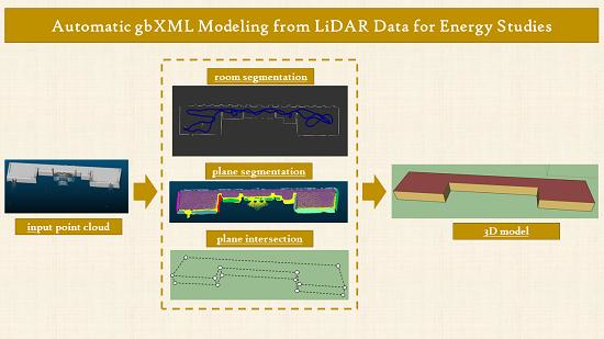
2.1. Geometric Modeling
Figure 1 shows the workflow applied for the geometric modeling of the building, prior to the generation of the gbXML schema. The procedure is performed in such way that the output (information about the walls) has the characteristics required by the gbXML format. That is: each surface is represented by its four vertices; adjacent walls have two vertices in common; each room is represented by a close space delimited by the walls and floor/ceiling. In addition, the process is defined for rooms within the same floor, in such way that the procedure should be repeated for all levels in multi-story buildings.
The process consists of a sweeping algorithm, where the point cloud is recursively analyzed until all points are classified within one wall and one room.
2.1.1. Room Segmentation
The first step of the process consists of segmenting the point cloud which is wanted to analyze in its different rooms. This strategy of the division of the point cloud in subspaces is followed by other methodologies [9], due to the simplification of the posterior geometrical analysis and the reduction of the processing time. Moreover, it is a requirement of the gbXML schema that each room is analyzed as a different element called “Space” [26]. The input data is a point cloud (in .las or .txt format) and the trajectory (in .txt format). The data from the point cloud and the trajectory that is required are the point coordinates and the timestamp of each point.
First, with the aim at reducing the computational cost of the process, a uniform downsampling is applied to the point cloud, decreasing the number of points of the point cloud to ¼. The optimal percentage of reduction has been decided after several experimental tests, with the aim at ensuring an improvement in the processing time without losing significant information for further processes.
The basic principle in which this process is based is that the element of separation between rooms is a door. The doors along the trajectory are detected with the following criteria: for each point of the trajectory, the points in the point cloud positioned below and at both sides are analyzed. When a significant reduction of the distances appears, both horizontally and vertically, this point of the trajectory corresponds with a door. Usually, more than one consecutive point is found for the same door. If these points are less than 1 m distance, the middle point is computed and designated as door point. The detection of the candidate door points must be supervised by the user, because some irregularities in the environment can also be interpreted as a door. Once the complete floor is analyzed and all doors are detected, the point cloud of the floor is segmented according to the different rooms. All points of the point cloud in a radius of 0.8 m from each door point are eliminated from the process. With this, one cluster of points is started for each room. The next step is to associate the points of the trajectory with each cluster, searching their coincidence in the horizontal plane. This way, the trajectory is segmented by rooms. Comparing the time stamp of each point of the trajectory, with the timestamp of each point of the point cloud, the points acquired from positions within each room are known.
2.1.2. Plane Segmentation
One characteristic of the gbXML schema is that only planar surfaces are accepted for representing the geometry of the building. This simplifies the models, while being enough for most energy analysis tools [23]. To detect the different planes in the point cloud a region growing segmentation algorithm implemented in PCL is used [27]. The most important parameters are the smoothness threshold (1º), the minimum cluster size (200) and the number of neighbors (50). These values, valid in our experiments, depend on the point cloud quality, and can be used in datasets with similar qualities of the point cloud (e.g., density, noise level, size). This segmentation typically results in an over-segmented cluster of planes. Planes with less than 200 points are omitted, reducing in this way the noise on the point cloud. Our interest is to obtain the planes of vertical walls and horizontal slabs (floors and ceilings) for each room. Surfaces from chairs, tables and furniture are considered as noise, since they do not contribute to the definition of the building envelope for energy purposes. Thus, with this value of the minimum number of points for each plane, the noise produced by complementary elements is reduced.
2.1.3. Plane Labelling
As mentioned in previous sections, the method proposed is restricted to Manhattan World Assumption without slanted floors and ceilings. All planes are considered perpendicular to the X, Y or Z axes. They will be referred to as YZ, XZ (vertical walls) and XY (horizontal slabs) planes. Each segment is classified in one of these groups.
The first step is to obtain the plane equation of each segment (Equation 1). The coefficients of the plane equation are calculated with PCL [28].
Ax + By + Cz + D = 0
With the plane equation of each segment, points are classified in planes as follows:
- XY planes
- |A| < 0.1
- |B| < 0.1
- 0.9 < |C| < 1.1
- XZ plane
- 0.9 < |A| < 1.1
- |B| < 0.1
- |C| < 0.1
- YZ planes
- |A| < 0.1
- 0.9 < |B| < 1.1
- |C| < 0.1
To filter the noise of the furniture of the room, the convex hull of each room is estimated, and all the point clouds that do not have points belonging to this convex hull are filtered.
Since each wall is only defined by one equation, all the segments corresponding to the same wall (result of the over-segmentation previously mentioned) are merged. To do this, the point cloud segments are compared to their equations for each group (XY, XZ, YZ). Near segments are candidates that belong to the same wall. The D coefficient of each equation for each group is analyzed as follows:
- /0< i < l where l is the number of segments of XY
- /0< j < n where n is the number of segments of XZ
- /0< k < m where m is the number of segments of YZ
All segments in a group are parallel to each other. Therefore, the absolute value of the difference between independent terms of the plane equation provides the distance between parallel planes. For example:
- /0 < i < n and 0 < j < n, where n is the number of segments in XY group, results in the distance between the ith and the jth elements of the group.
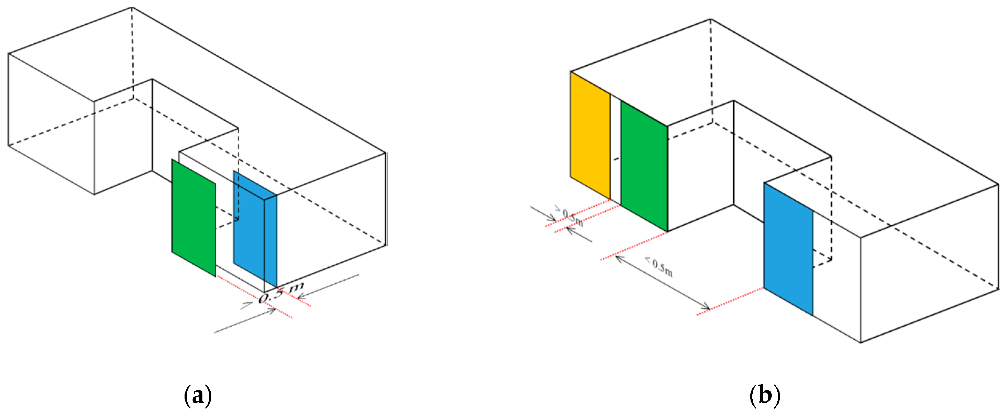
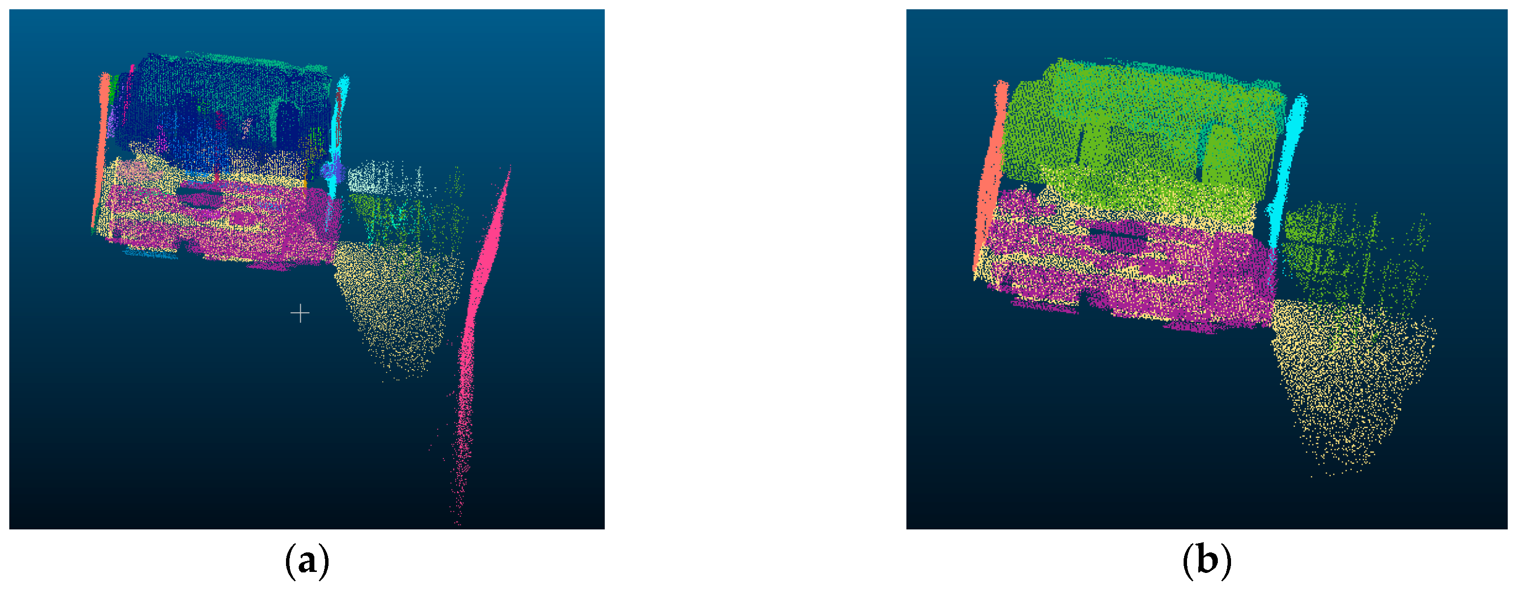
Thus, for each group, if /0 < i < n and 0 < j < n, where n is the number of elements in the group, the ith and the jth elements are candidates to belong to the same wall (Figure 2a). Then, the minimum distance between the bounding boxes of each candidate is analyzed, and if it is smaller than 0.5 m, the segments are considered as the same wall, and both point clouds are joined in one (Figure 2b). Every time there is a coincidence of segments, the new point cloud is compared with the rest of the elements. This wall clustering needs the validation of the user. Once all the segments of the group are analyzed, the equation of the final walls is recalculated.
2.1.4. Planes Correction
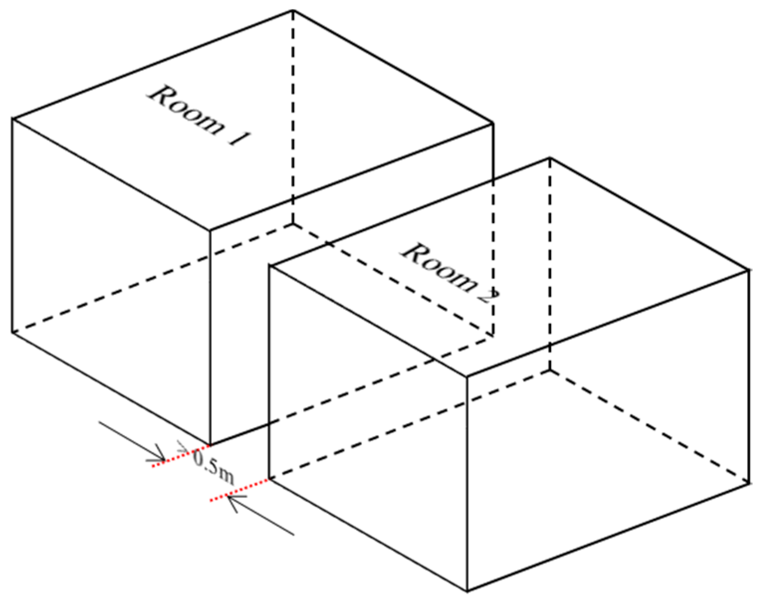
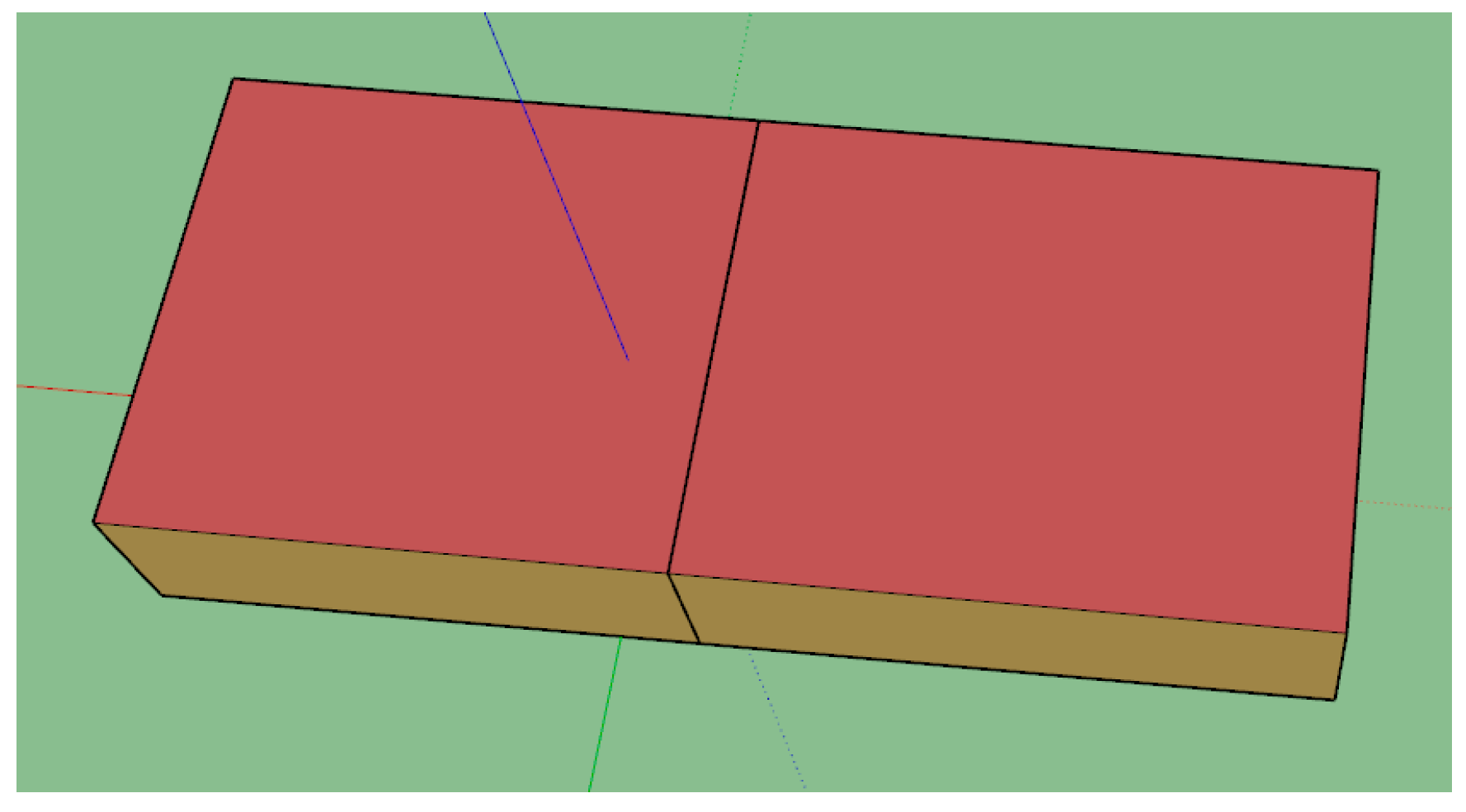
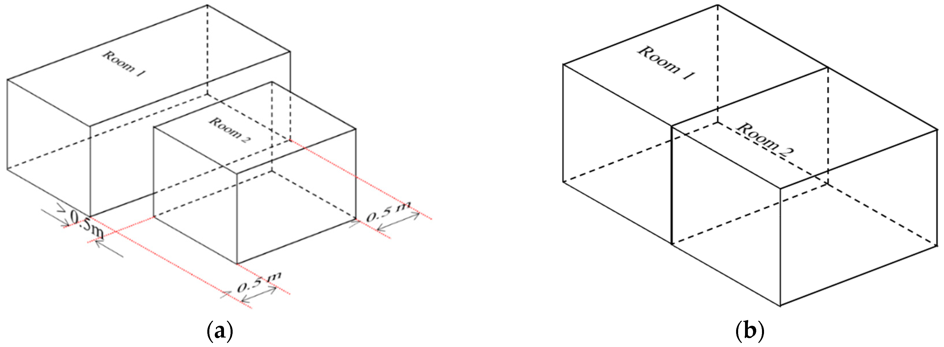
The previous process is repeated for each room, in such a way that the walls and their planes are obtained for each room. Nevertheless, the objective of the methodology is to generate a gbXML file including all the rooms acquired. Figure 3 represents an example of separated walls that should be merged into one, in order to have a close space for the gbXML product. The reason for the computation of different planes from the same wall is the wall thickness, but the thermal analysis requires that walls are defined as polygons with no thickness. Thus, the medium plane between these walls is estimated and used for both rooms. This process needs the validation of the user.
2.1.5. Wall Intersection
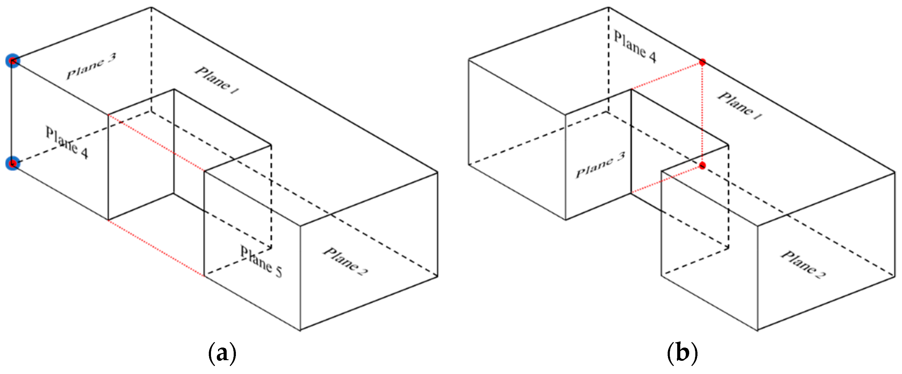
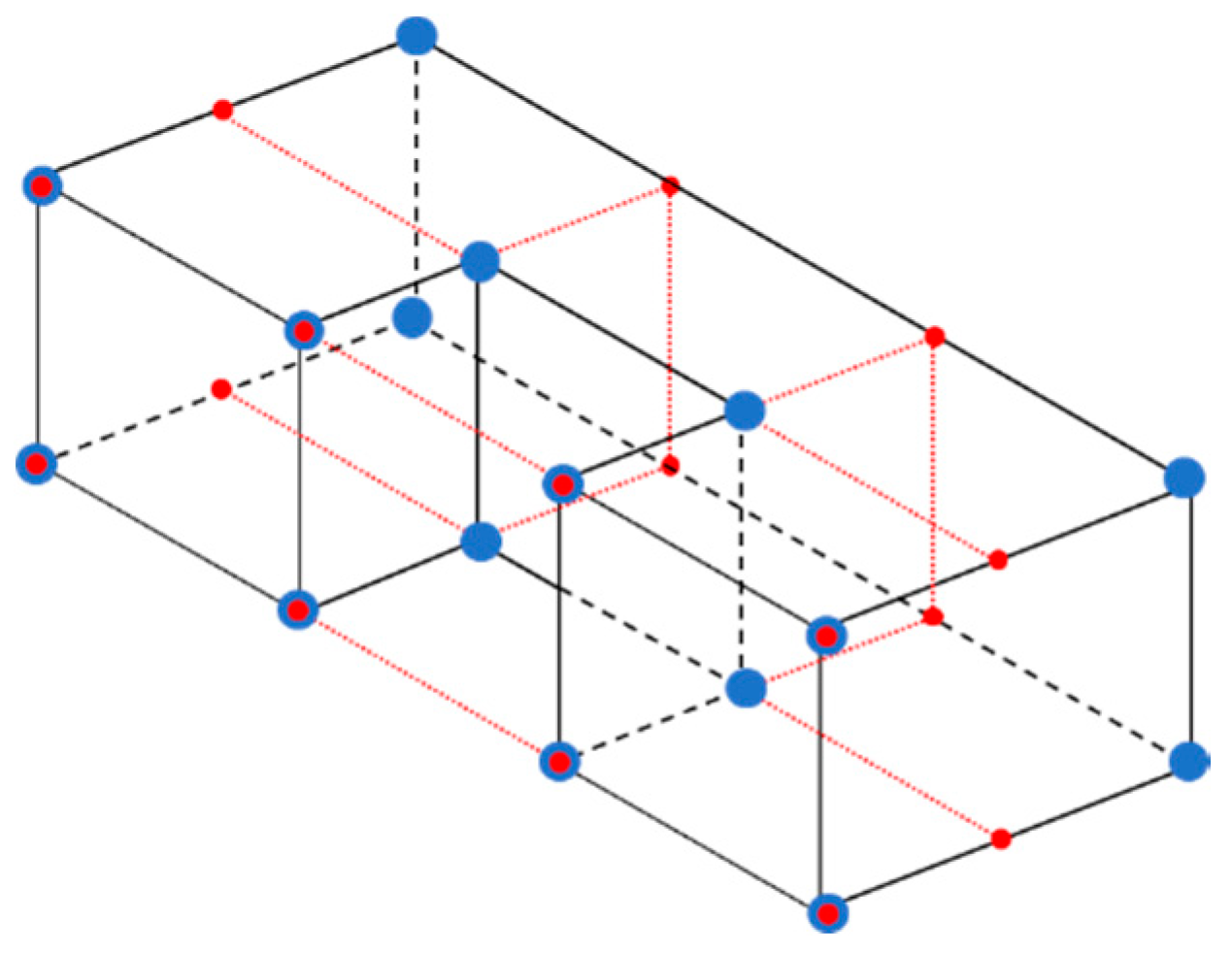
As mentioned before, each geometric element of the building in gbXML is represented as a plane surface. This surface is defined by its vertexes [26]. Several methodologies intersect the estimated surfaces of the building to obtain the basic elements which characterize the model [11,29]. For this methodology, the intersection points of every wall from each group with the walls of the other groups are computed (the intersection of three non-parallel planes results in a point). The points obtained this way are named as “virtual intersections”. These points need to be filtered to obtain the vertexes of each wall, because the intersections of the planes with their equations are estimated without testing the existence of a contact between the walls. In some cases (Figure 4a), the presence of different walls with the same equation results in the presence of duplicated virtual points. In other cases (Figure 4b), the prolongation of one wall creates virtual points in the middle of the perpendicular wall.
2.1.6. Vertex Estimation
The assumptions required for the gbXML generation are that each vertical wall is a rectangle and each horizontal slab can be an irregular polygon, but coincident with its respective floor or ceiling. Therefore, each wall must be defined by four vertexes. This assumption is used to filter the virtual intersections and obtain the real vertexes of each surface. Another important assumption is that the points of each group (XY, XZ, and YZ) must be the same, but classified in different walls. The closest walls of each group are obtained from virtual intersections of groups XZ and YZ. If there is a coincidence between the closest walls and the walls intersected to obtain the virtual point, this virtual point is considered as a real vertex. Vertexes from groups XZ and YZ must be the same. Then, these vertexes are compared with the virtual points from group XY, excluding the non-coincident ones. This process needs the validation of the user.
2.1.7. Wall Correction
As done in Section 2.1.4 with the planes of the walls, the estimated polygons that correspond to the two sides of vertical walls common between rooms need to be defined as one. This is a requisite of gbXML schema [30]. Four different issues can appear (Figure 5):
- Both polygons are equal: this is the simplest case. Only one of the polygons is required. Thus, the second is eliminated (Figure 5a).
- One polygon is contained in another but with one of the vertical edges in common: the smallest one remains without changes. The biggest one is divided into two different polygons, which correspond with the common and uncommon part (Figure 5b).
- One polygon is contained in another but without vertical edges in common. The big polygon is divided into three, one which corresponds with the common part and the other two with the uncommon parts (Figure 5c). The small polygon remains as one.
- Both polygons have in common a part of their area without being contained one in another: the two polygons are divided in a total of three, which correspond with the two uncommon areas and the common area (Figure 5d).
2.2. GbXML Generation.
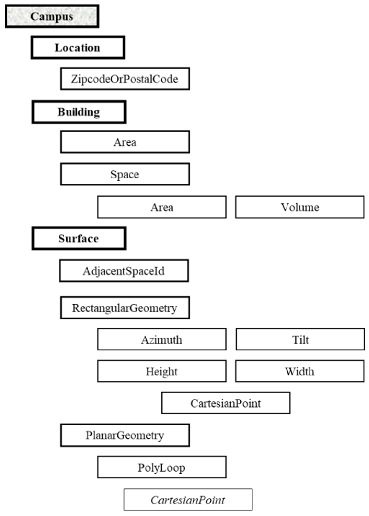
The essential data for the 3D modelling were presented in previous subsections. These data are the core of the gbXML file. The geometry of each wall, ceiling, or roof in gbXML format is defined by their vertexes, which have been estimated before. Moreover, in the software, each point is associated with the containing surfaces (each point belongs to three surfaces), and each surface is associated with the containing spaces (one surface can belong to two spaces at the same time, as explained before). The basic structure of this file is shown in Figure 6.
The gbXML file is generated using the Qt classes for XML handling, specifically, QDomDocument, QDomElement and QDomText [31]. Each of the elements of the graph in Figure 6 represents a node.
- Campus: this node is used as base for all physical objects. It has an attribute called “id” which has the value “Campus_0” by default.
- Location: this node has a child-node called “ZipcodeOrPostalCode”. The value of this node is written by the user using the developed interface. The value is introduced in the field called “Código Zip”.
- Building: the software only writes one Building node in each gbXML file, because the analyzed point cloud belongs to only one building or to a part of it. It has two attributes: “Name”, which is introduced by the user in a field called “Nombre” and “buildingType”, which is selected by the user in a field called “Tipo”.
- Area (from building): is the summation of the area of the floors of each space of the building.
- Space: each space corresponds with one room. Each space has an attribute called “id”, which is appointed with the value <“Space” + index of the room in the data structure of the software>.
- Area (from space): area of the floor of the room. It is estimated as the area contained by the vertexes of the corresponding floor.
- Volume: volume of the room estimated as the area of the floor multiplied by the height of the ceiling.
- Surface: each surface corresponds with one wall, ceiling, or floor of the building. Each node has two attributes. The attribute “id” is set as <“Surface” + index of the surface in the data structure of the software>. The attribute “surfaceType” is set as “ExteriorWall” except for those that divide adjacent rooms; in which case they are set as “InteriorWall”, “Roof” or “SlabOnGrade” depending if the surface is a wall, a ceiling or a floor.
- AdjacentSpaceId: each surface has as much “AdjacentSpaceId” as spaces to which the surface belongs. Their value is the “id” of the corresponding space.
- RectangularGeometry: this child-node from each surface defines the overall geometry of the surface.
- Azimuth: the value of this node is estimated based on the value introduced by the user, using the interface, in a field called “Azimut”. This value is the reference value of azimuth for the Y-axis, which has the relative value of 0º. Therefore, walls with normal vector coincident to the positive X-axis have 90º, and 270º if the normal vector is coincident with the negative X-axis. Walls with normal vector coincident with negative Y-axis have azimuth equal to 270º. Azimuth 0º is assigned to horizontal slabs. The relative value is added to the reference value to estimate the azimuth of each surface.
- Tilt: assuming Manhattan World, the value of the child-node “tilt” from “RectangularGeometry” is 0º for horizontal planes and 90º for vertical planes.
- Height: this child-node from “RectangularGeometry” is estimated as the absolute value of the difference between minimum and maximum z value of each wall, except for horizontal surfaces, where height is the absolute value of the difference between the minimum and maximum y.
- Width: this child-node from “RectangularGeometry” is estimated as the area of the surface divided by the height.
- Cartesian point: this child-node from “RectangularGeometry” corresponds with the second point of the list of points for each surface.
- PlanarGeometry: this child-node from “Surface” defines the geometry of the surface.
- PolyLoop: list of the vertexes of the surface ordered counterclockwise.
- CartesianPoint: this child-node from “PolyLoop” corresponds with each vertex of the surface.
- Coordinate: this node corresponds with each coordinate of the point.
Once all nodes of the XML schema are created and completed, the file is written, saving the results.
3. gbXML Results and Energy Applications
3.1. Case Studies
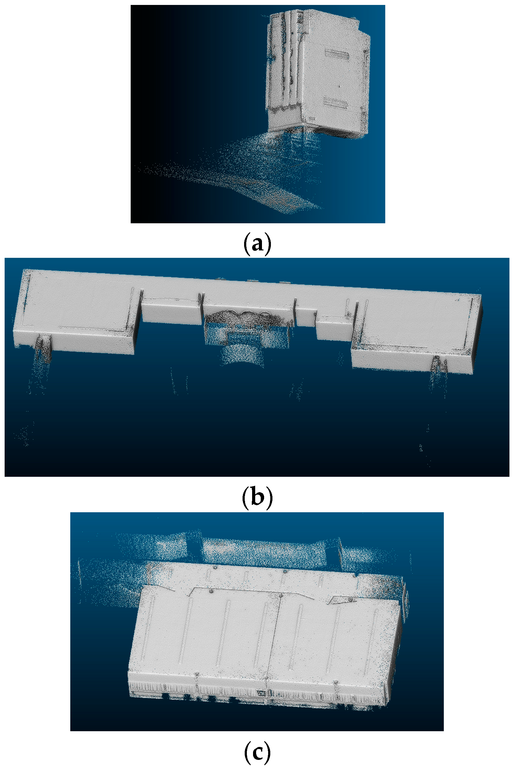
The performance of the developed system is presented through its application to 3 different real-world cases of study with increasing complexity, but simple enough to understand and test the performance of the algorithm. The three scenarios used to test the system are presented below.
The first one is an independent room. It is the simplest one (Figure 7a), but allows one to illustrate the simplification process for gbXML schema and work in small scenarios. The second is an independent room with a structure that can be used an example of how to detect the vertexes of the space (Figure 7b). The third (Figure 7c) is composed of a corridor and two classrooms and complements the previous examples with the room segmentation algorithm. All examples are made on data acquired with the 3D Scanner Zeb-Revo [32]. The cases of study correspond to the cases 1 and 2 from Section 2.1.7 (Figure 5a,b).
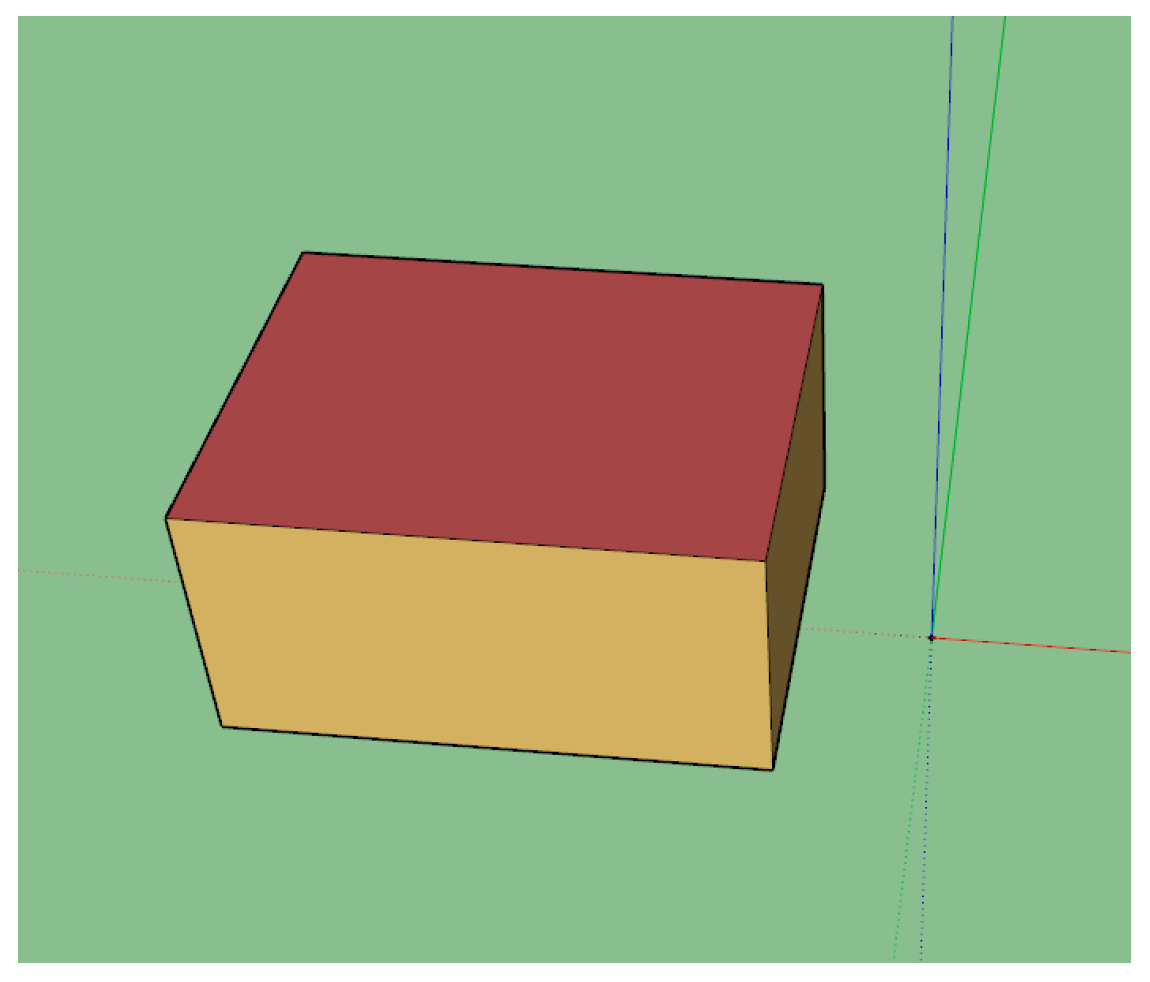
The first case is the simplest example. It is the smallest one, with 15.15 m2. It is selected to test the basic performance of the system. It is entirely captured from the inside of the room. Therefore, the room segmentation algorithm only detects one room. However, some noise points are acquired in the exterior of the room, associated with the same space. This is produced because the door was open in the time of surveying, and these points are associated with the room by their timestamp and the timestamp of the trajectory. This noise is filtered by the system, and the geometry is regularized and simplified. Moreover, the noise produced by the furniture inside the room is filtered too. The estimated 3D model in SketchUp is shown in Figure 8.
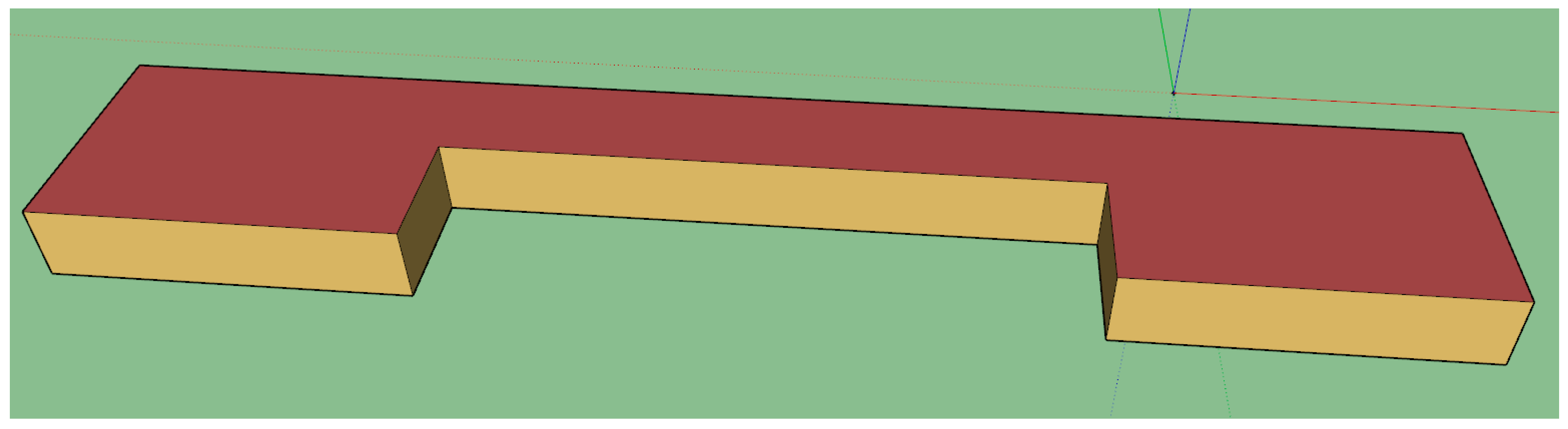
The second case presents the same problem with noise acquired across an open door (in this case, a gantry). It also presents some noise produced by the windows in one of its walls. Its bigger size of 533.26 m2 allows one to test the association algorithm between segments of wall explained in previous sections under worse conditions than in case of study 1. The geometry of this example is interesting to test the algorithm of detection of vertexes because of the non-convex form of this floor. The 3D estimated 3D model in SketchUp is shown in Figure 9.
The last case consists of two laboratories (one of 114.5 m2 and the other of 99.5 m2) and a corridor, but the corridor is only partially captured. Therefore, it is detected as another room during the room segmentation step, which is omitted to the geometrical analysis. This example is used for the development of the procedure for incomplete or erroneous surveys. The interest for this is to generate a robust methodology to be applied in real cases of study, and consequently should be capable of dealing with some uncertainty. The point cloud also presents noise because of the glass surface of one of the walls of the corridor. The estimated 3D model in SketchUp is shown in Figure 10.
3.2. Energy Application Example
In this section, the utility of the models obtained for thermal analysis purposes is demonstrated through their use for the simulation of the energy consumption by heating systems installed in each building along a year. The tool used for the simulation is OpenStudio [33], which uses the calculus engine EnergyPlus, launched from SketchUp. The same example is performed in all three models, for comparison purposes, focusing on the effect of the geometrical representation on the computation of energy consumption more than in the reality of the construction (materials, presence of pathologies, etc.).
Some requirements should be followed for the correct simulation of the model. First, the Space Types should be defined in SketchUp. All examples are defined as “office”. Then, the attributes of the space should be defined, such as the ASHRAE Climate Zone, although it can be modified later.
With this input, OpenStudio can be launched. The weather file of Pontevedra is loaded, which is the location of the three cases of study (with the extension “.epw”, which comes from EnergyPlus Weather). This file includes the weather of the place and its geographic coordinates. The system requires an indication of which parameters are required in the estimation, which in this study, are ideal air loads of the building. These need the prior definition of the thermostats of the building. Following these steps, the energy consumption of the heating systems during a year is calculated. The results seem coherent. With the same conditions, the consumption depends on the volume of each Scenario, as seen in Table 2. Therefore, the highest values of maximum consumption and mean consumption go to Scenario 2. If the values of maximum consumption per volume and mean consumption per volume are analyzed, Scenario 2 and Scenario 3 practically show the same values. It can be supposed that with higher values of volume, the analysis is more stable. The fact that having multiple rooms instead of one seems not to interfere in the analysis is remarkable.
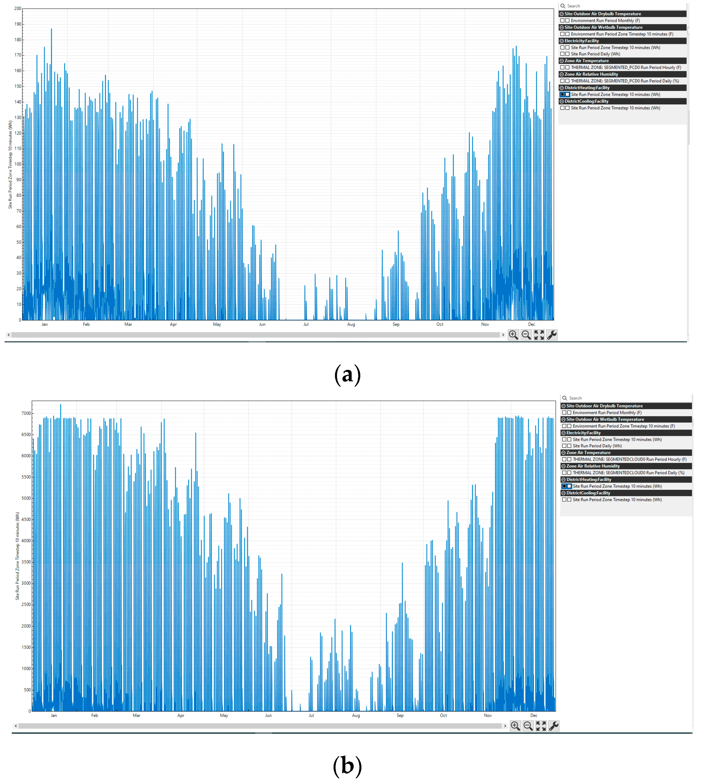
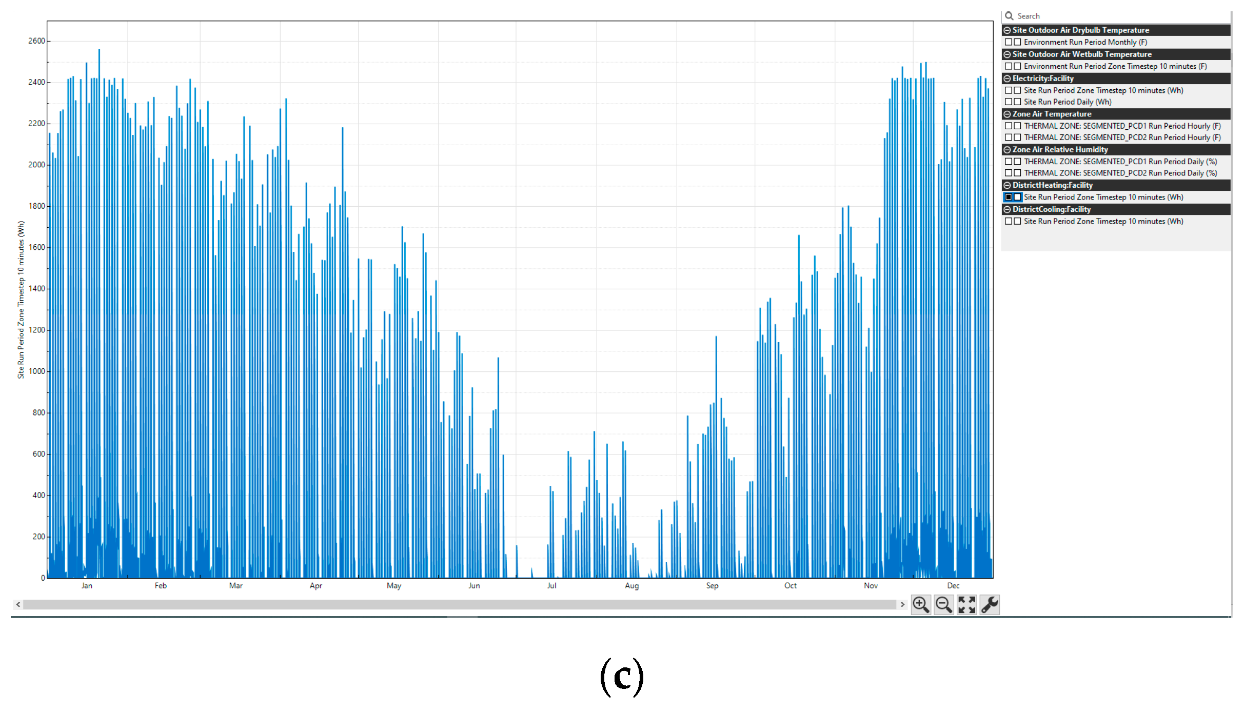
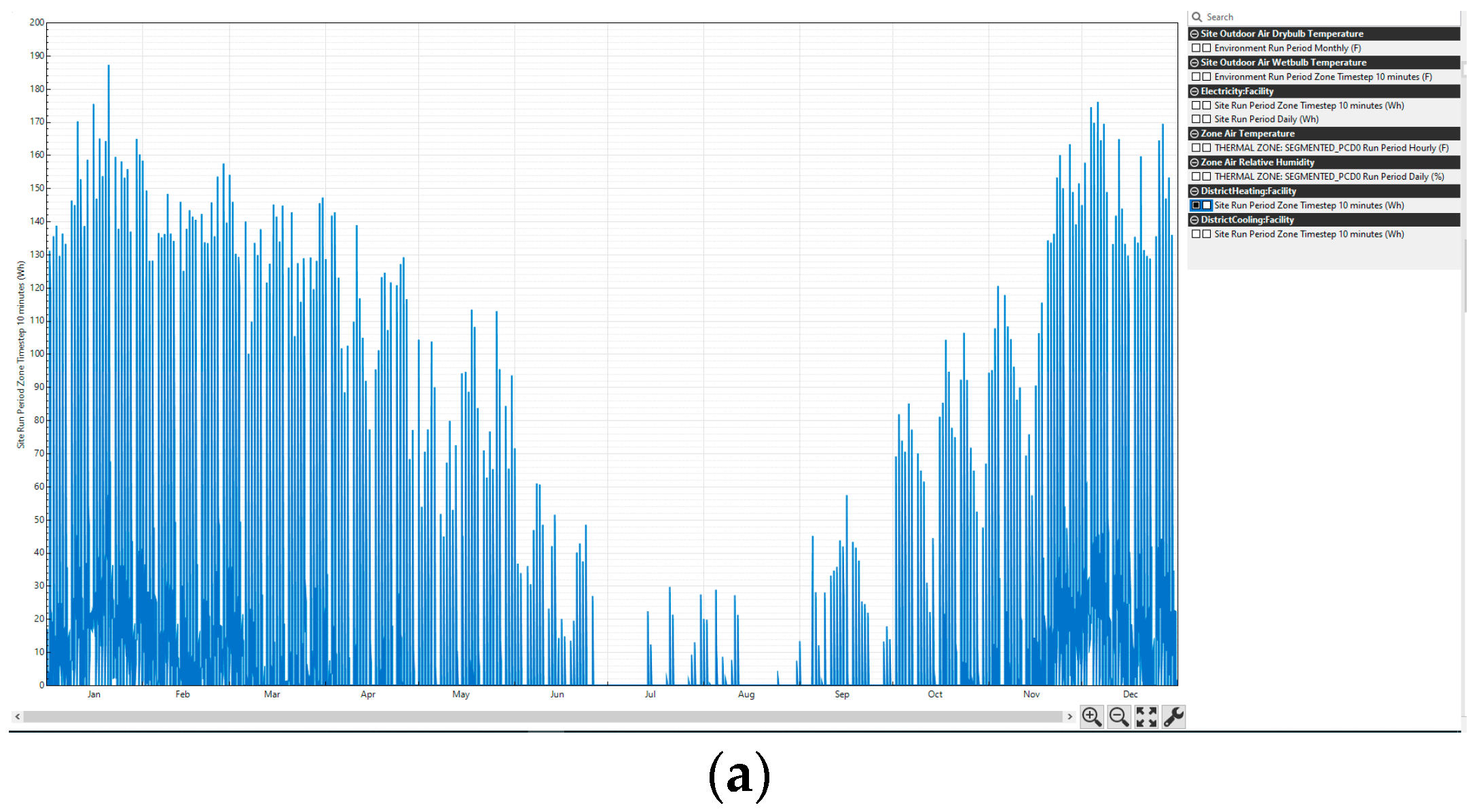
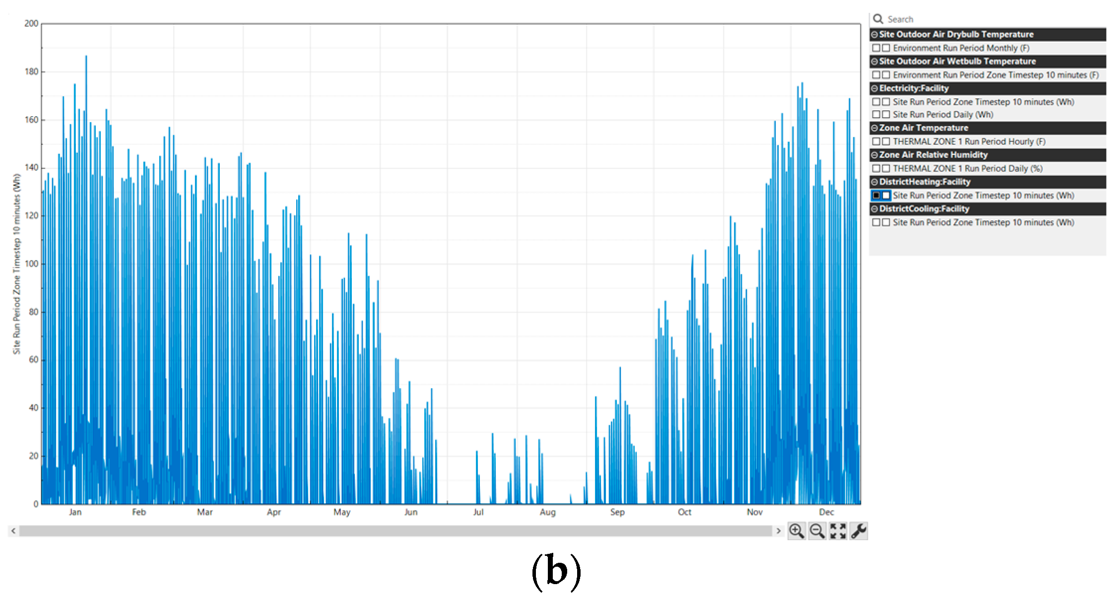
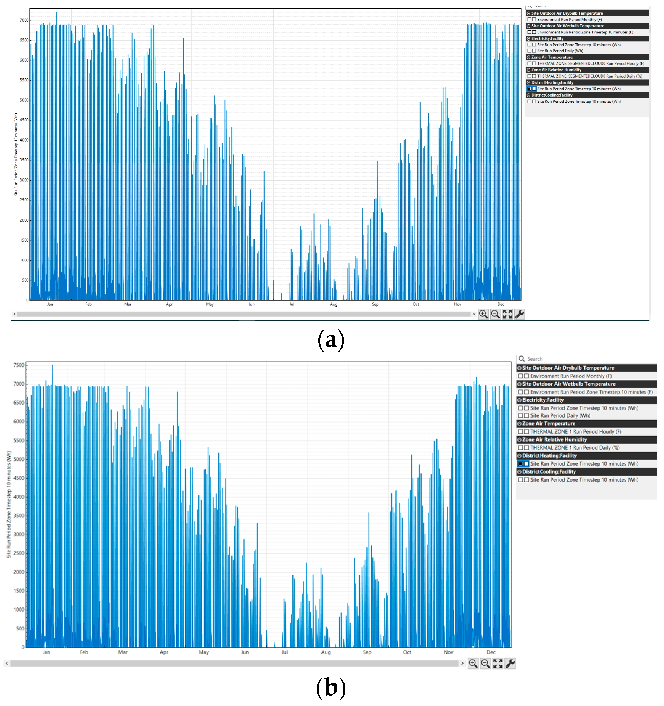
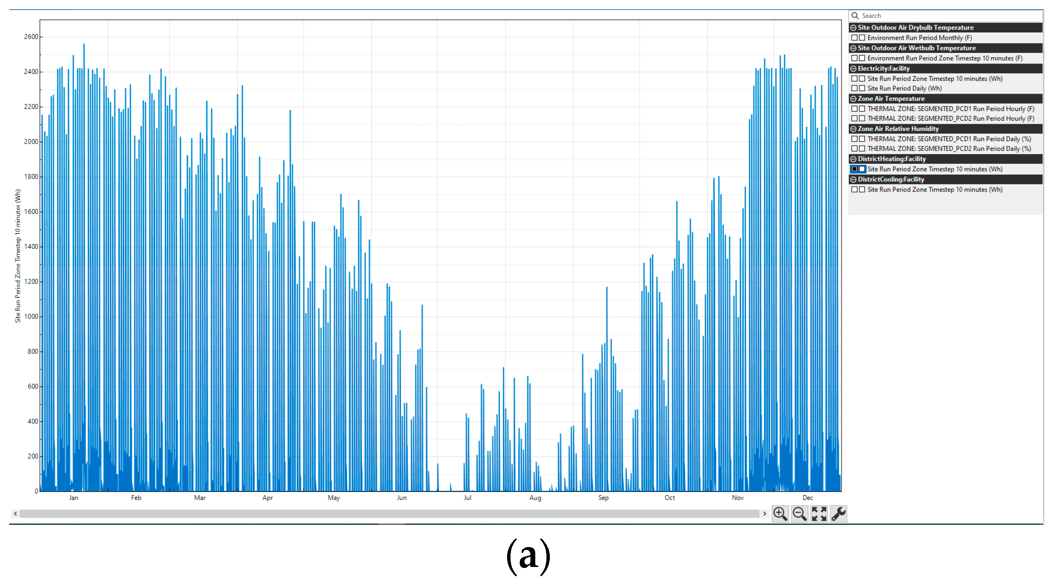
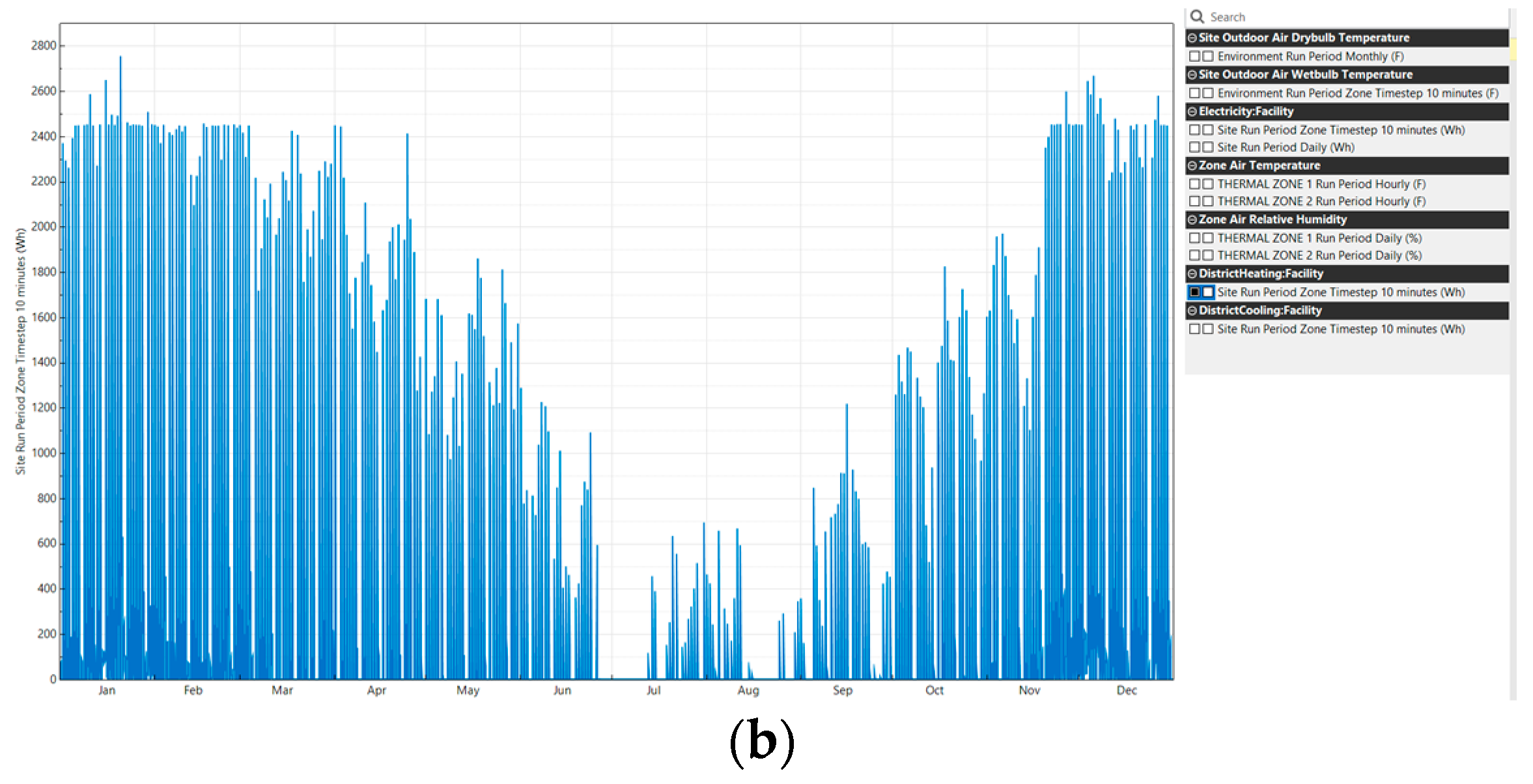
Figure 11 represents the consumption of the heating systems along a year for each scenario. It can be observed that, without the oscillation in the values, the three graphics are very similar, having a lower consumption in the months of summer (specifically at the start of July and August) and a higher consumption in the winter. All graphics sow their consumption peak in January. As it is said before the form of the three graphics is practically the same, displaced along the vertical axis. This is explained because, assuming the three scenarios in the same location, the behavior of the heating system must be the same. As said before, the value of the consumption depends on the volume of the scenario, but the temporal behavior is the same.
4. Discussion
4.1. Analysis of Performance of the gbXML Generation Method
In this section, the performance of the method for each case of study is evaluated. The critical points in the flux of the systems are the clustering of plane segments for obtaining the walls, followed in order of importance by the room segmentation. These processes require the attention of the user, to verify or correct the results obtained. Their successful outcome determines the success of the whole gbXML generation process.
The point clouds are surveyed with a Zeb-Revo, which has an accuracy of 0.03 m [34], which determines the accuracy of the input point cloud. The experiments were run on Ubuntu 16.04 LTS, with an Intel Core i7 CPU an NVIDIA GF119M GPU. The summary of the results of the three scenes can be seen in Table 3.
Case 1 is the simplest one. Therefore, there are practically no problems during the execution of the software and the user only needs to confirm each step. The point cloud of the room has a size of 4302130 points and the point cloud of the trajectory, 13100. The survey was made from the inside of the room. Thus, the room segmentation algorithm does not detect any door along the trajectory in 27 s (Figure 12).
The point cloud is voxelized with a size of the side of the voxel of 0.03 m. This value is obtained by experimentation to reduce the processing time without losing the information. The plane segmentation algorithm is performed for the detected room. The parameters of the region growing algorithm are: minimum size of detected planes of 200 points, the size of the neighborhood is 50 points and smoothness of 1º. With these parameters, 32 planes are detected in the room in 6 s (Figure 13a). These planes are classified as XY, XZ and YZ planes and merged by their proximity, as was explained in the previous section, obtaining 2 XY planes, 2 XZ planes and 2 YZ planes (Figure 13b). They intersect obtaining 8 intersection points, which are used to generate the gbXML structure. The entire process lasts 94 s, but this value is relative in this case, because it depends on the time that the user last validated each step.
Case 2 is more complicated, given its geometry and dimensions. The room segmentation algorithm detects only one room in 110 s (Figure 14).
Due to the larger size of the point cloud (the point cloud of the room has 13,647,747 points and the point cloud of the trajectory, 39,237), this case is voxelized with a size of the side of the voxel of 0.08 m. As in the previous case, the room segmentation algorithm only detects one room in 110 s. The plane segmentation algorithm of the room uses the same parameters as in the previous case. The algorithm detects 93 planes in 25 s (Figure 15).
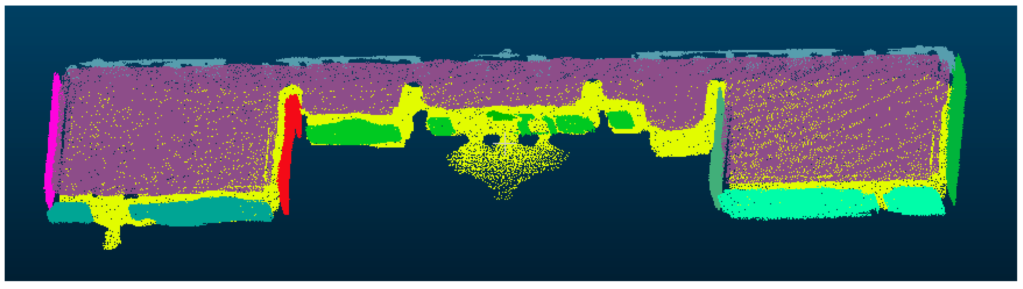
From them, 13 XY planes, 41 are XZ planes and 22 are YZ planes. The correction of the planes, in this case, obtain 2 planes XY, 15 XZ and 8 YZ. These values are unacceptable, but can be repeated, changing the values of the correction algorithm. For the planes XZ, it is repeated with a distance between groups in the same plane of 3.5 m, obtaining 8 groups XZ. All planes are then correct, but some of them are produced by the great noise of the point cloud. This noise can be seen in Figure 16 as the segments of point clouds on the top of it. The undesired groups can be corrected by the user obtaining the needed 4 XZ planes for the desired simplified 3D model. The association of planes for YZ planes is correct, but some of the estimated groups are produced by planes that must be omitted to obtain the simplified model required for this example. The user can correct the groups, selecting the needed 4 groups (Figure 16). Then, the groups are intersected, obtaining 16 intersection points, which correspond with the vertexes of the model.
After the correction made by the user, the segments of Figure 17 are obtained. Each color corresponds to a different wall. The system works well with the floor and ceiling of this case, but needs to be corrected for walls, especially the longitudinal ones.
When the planes of the walls are intersected (2 from group XY, 4 from group XZ and 4 from group YZ), 32 intersection points are obtained. This is produced, as shown in Section 2, because of the intersection of some planes, which have a mathematic intersection but no real contact between the walls represented by them. Thus, the estimated virtual intersection points are 32, but after evaluating which of these points are vertexes, an amount of 16 real vertexes is obtained. In Figure 17, a schema of the problem for this scenario is shown. Although this part of the system is supervised by the user and needs his approval, it is tested that no problem appears if the previous clustering process is correct.
Once the real vertexes are estimated, the gbXML schema can be generated. The whole process with user interactions lasts 407 s.
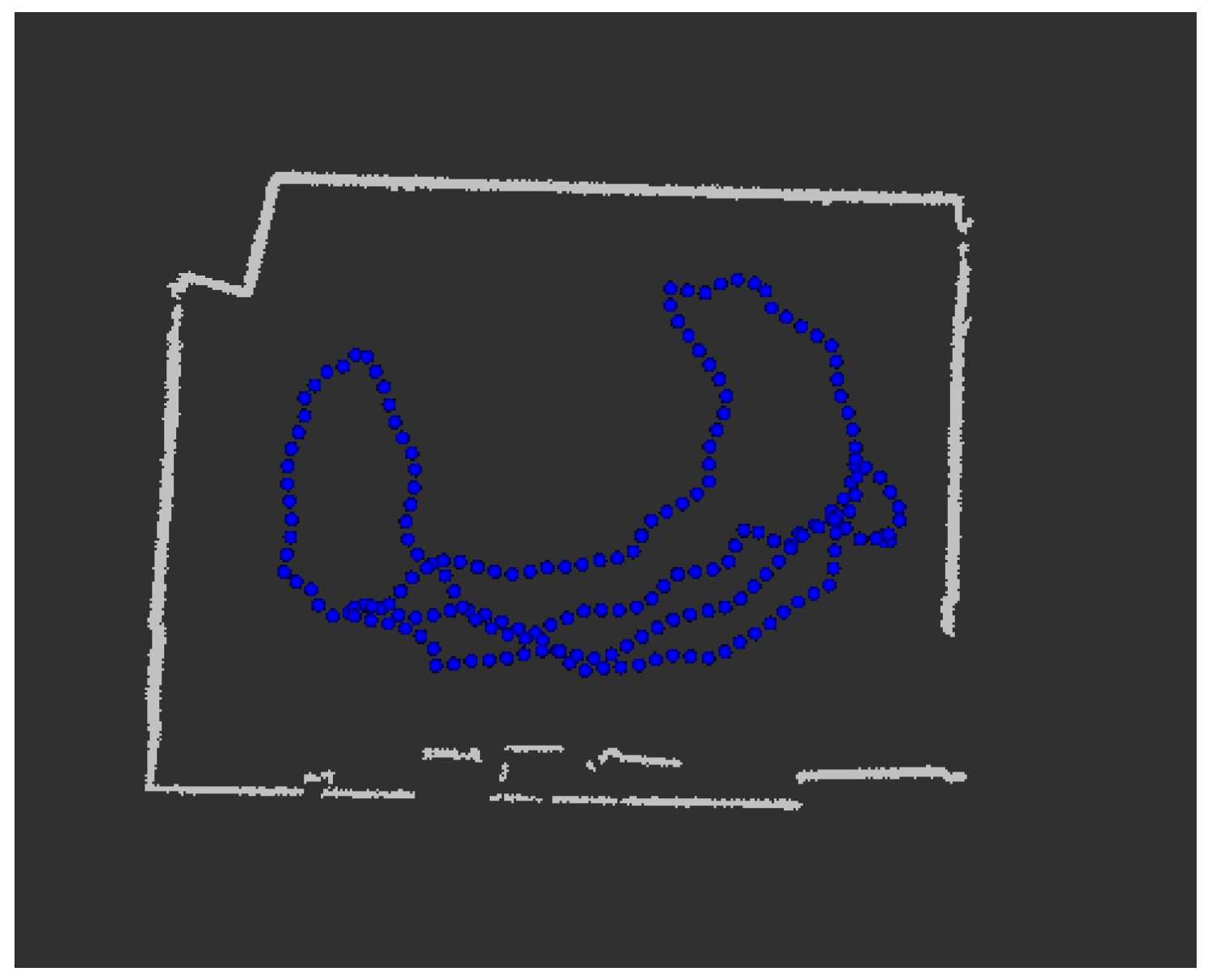
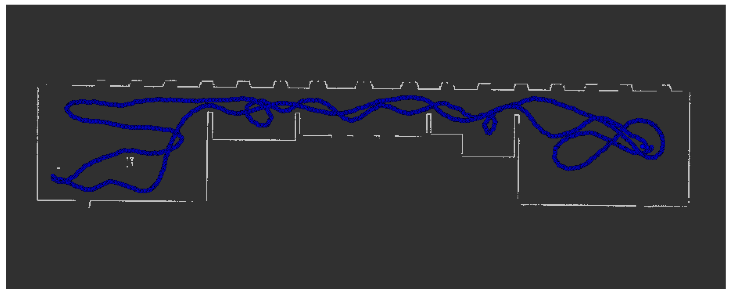
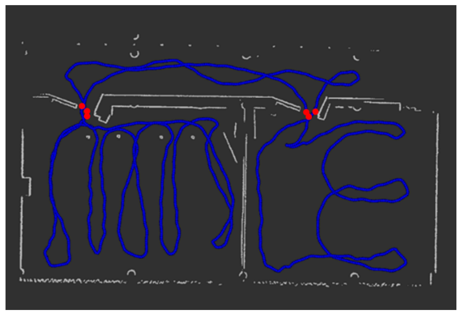
In case 1 the basic performance of the algorithm is studied. Case 2 enables the study of how the system deals with more complex geometries. Case 3 allows one to test the performance with multiple rooms and how to deal with errors on the acquisition of one of them. The input point cloud corresponds with two rooms and a segment of the corridor with a size of 11,156,807. The trajectory point cloud has 33,265 points. Working with non-ideal scenarios allows one to think about how to solve the problems inherent from the data acquisition and its processing, as will be explained with Scenario 3, making the system more flexible. The system allows selecting the rooms that the user wants to analyze, avoiding the incomplete or corrupted ones. As shown in Figure 18, the room segmentation algorithm detects two doors along the trajectory in 86 s, splitting the input point cloud among three different rooms. It is not strange to find multiple near points of the trajectory identified as a door. It must be considered that the survey was performed making loops in the trajectory, and each door was crossed two times minimum. Moreover, because of the geometry of the doors and the trajectory of the acquisition, multiple near points are susceptible to meet with the conditions of a door. That is why a radius of 0.8 m is considered from each door point to replicas of this door.
As mentioned before, the corridor is incomplete, and cannot be reconstructed. Thus, in the GUI of the methodology, the user is given the option to select which rooms to analyze, in case of issues during the acquisition. Therefore, only the two rooms present in the corridor are analyzed.
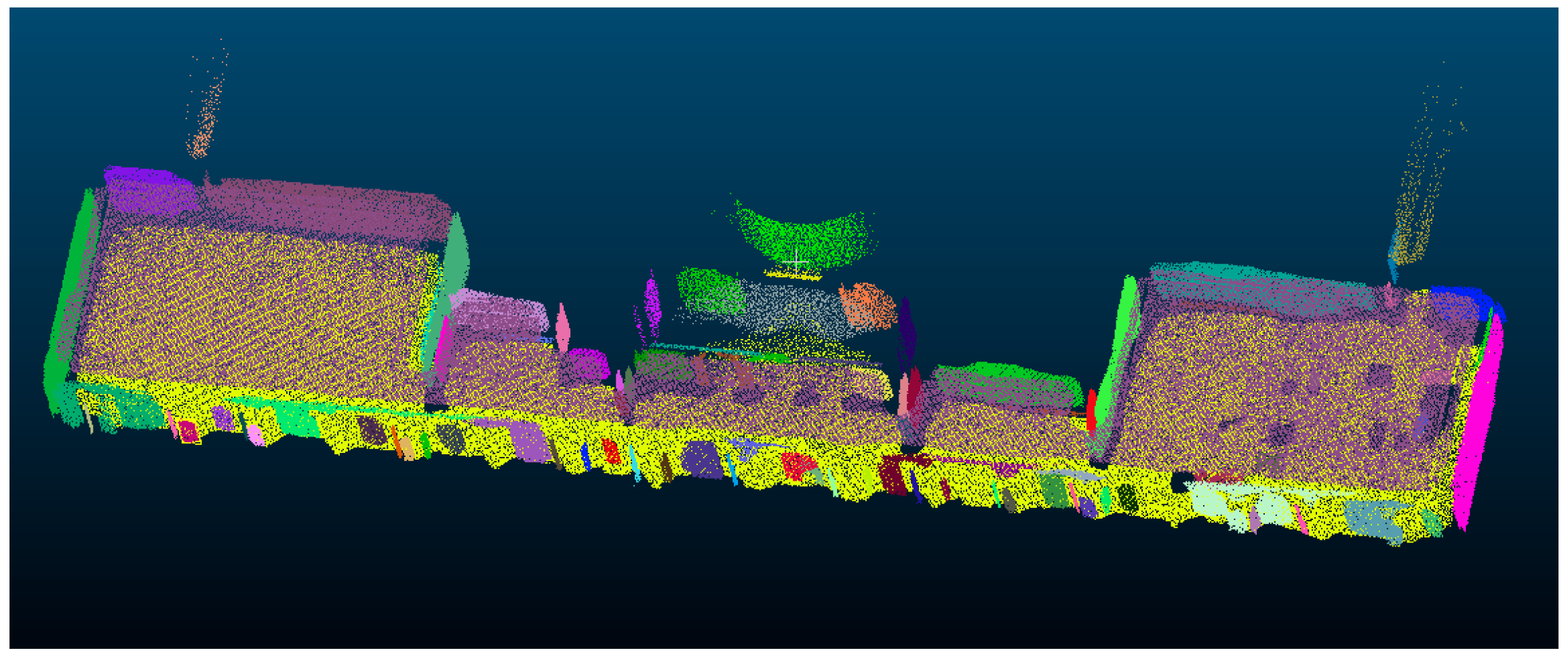
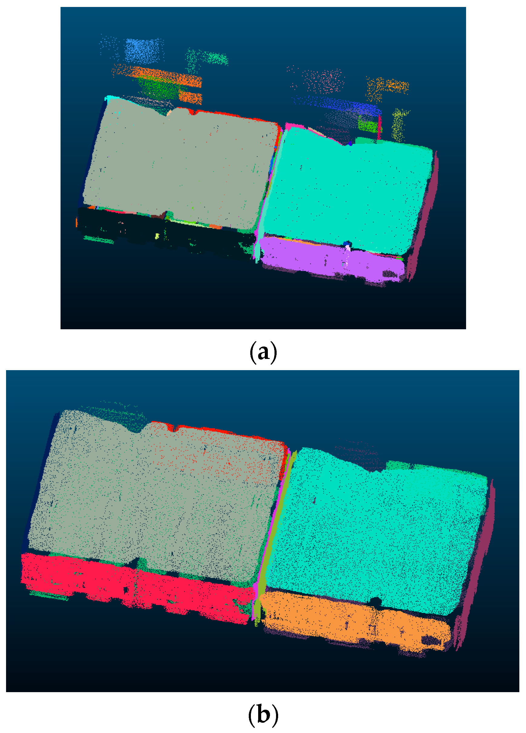
The room segmentation algorithm detects 3 different rooms in 86 s. The segment of the point cloud which corresponds with the corridor is incomplete. Therefore, it is discarded for the rest of the process. The other two segments of the point cloud are voxelized with a side of a voxel of 0.03 m. Each room is segmented in planes with the same parameters, as in the previous cases. One of the rooms is segmented in 63 segments in 19 s (Figure 19a). From these planes, 17 are XY segments, 11 are XZ segments and 6 are YZ segments. The correction planes algorithm obtains 2 groups of XY planes, 4 groups of XZ planes and 2 of YZ planes. From the XZ groups, 2 must be discarded by the user because they correspond with reflected surfaces, as can be seen in Figure 19a. For the other room, 73 segments are obtained in the plane segmentation. Fifteen of them are classified as XY planes, 10 of them as XZ planes and 14 of them as YZ planes. The planes correction algorithm obtains the same results as in the other room. The correct clusters can be seen in Figure 19b.
Following the workflow described in Section 2, now all adjacent planes are corrected as shown in the schema of Figure 20. Of course, the schema is exaggerated to show a better visualization of what happen between the two rooms. The medium plane between the adjacent parallel planes is calculated to regularize the model and remove the gaps between adjacent rooms.
At this point, the planes of each room are intersected. With 6 planes per room, 8 intersection points are obtained, which are the vertexes of each room. After generating the gbXML schema with these data, one last correction is needed, as explained in Section 1: if any wall corresponding with the intersection wall between two rooms is duplicated, one of the polygons is deleted for this wall and the polygon left is used to define the wall for gbXML. This polygon is assigned to the two adjacent spaces, one for each adjacent room. The whole process with user interactions lasts 427 s.
After comparing the time of the process in the three cases, time shows to be highly dependent on the number of points of the point cloud of the scenario. Attending the duration too, the critical step is the room segmentation. It is followed by the plane segmentation of each room and the plane classification and correction.
To evaluate the accuracy of the system, the 3D models of the scenarios have been manually elaborated to compare with the 3D models estimated by the software. This way, the system is compared with the traditional methods. The 3D models in SketchUp can be seen in Figure 21.
Table 4 shows the error estimation of the areas, using as reference value, the areas of the manually elaborated models. The best performance goes to Scenario 3, particularly to room 1.
Table 5 includes the volumetric comparison between the estimated models and those manually elaborated. All the errors estimated are satisfactory, remaining the relative error below 1.3% in all cases.
The system worked well in all three scenarios with satisfactory errors, and the only remarkable problem during the execution was the reflected surfaces, which can be solved by the user interaction.
The energy analyses performed in the previous section have been repeated with the handmade models. The results can be seen in Table 6. The results are coherent with the results for the estimated models. The biggest scenarios have practically the same maximum consumption per volume and mean consumption per volume. Moreover, these values are very similar to the obtained for the estimated models, showing the same tendency.
The comparison of the behavior of the consumption of the heating system along a year can be seen below in Figure 22 for Scenario 1, Figure 23 for Scenario 2 and Figure 24 for Scenario 3. It can be seen in the graphics that the behavior for the consumption is the same for the estimated cases than those used as a reference. The form of the graphics is practically the same, only with slight variations in the peaks of consumption value. The months of maximum and minimum consumption remain equal and their values are similar.
4.2. Comparison of the Proposed Method with Existing Methods
Compared to related work, the proposed system presents the advantage of controlling the workflow of the process, avoiding the propagation of errors and making it affordable for non-specialist users. A general comparison with the related work is difficult because of the variety of the scenarios and the purposes of each system. However, a brief comparison explaining the advantages and disadvantages of each system will be performed, based on the available data. Ambrus et al. [7] present an efficient and robust fully-automatic method for indoor 2D reconstruction, without prior knowledge of the scanning device poses. This method can also detect and categorize gaps in the structure, like doors. However, 2D reconstruction is not compatible with energy analysis, which is the use for the models of the proposed system. Moreover, their system is designed to work with rooms which tend to be convex, whereas the proposed system can work with concave rooms. Wang et al. [8] present a framework for 3D modelling of indoor point clouds acquired with mobile laser scanners. Their system uses the 2D projection of the point cloud to detect the walls of the building and generate 2D floor plans and 3D watertight building models. Their system was tested against synthetic and real-world scenarios, presenting a maximum average error in the distance between the detected planes and their closest point of 3.528 cm. Their system is also able to reduce the effect of outliers and small structures, like irregular bumps and craters in the 2D floor plan. The doubt about the performance of the system comes in the case of point clouds with clutter from furniture like large wardrobes. The reason for this doubt is that the method proposed in [9] can easily detect erroneous surfaces as primitive of a wall in crowded rooms. In contrast, the method proposed in this paper allows the user to control each step of the process, allowing for the detection of irregularities that can appear in real-world scenarios. Macer et al. [9] present a semi-automatic approach for 3D modelling, using indoor point clouds. Their choice as schema for the 3D model is IFC, and it can work with different floors. Their approach divides the input point cloud into different sub-spaces, with one point cloud per room, analogously to the method proposed. This strategy simplifies the logic of the 3D reconstruction. Their approach was tested against two different scenarios, resulting in the generation of 3D models with satisfactory accuracy: 4.4 cm is the maximum deviation from the control points. Therefore, the operation times in [9] are 8 min for scenario 1 with ~10M points and 19 min for scenario w, with ~39M points. Thus, the method proposed is slightly faster. Murali et al. [10] present an automatic system to generate BIM of indoor point clouds which is remarkable for its speed. Their system was tested, with five real-world scenarios being able to generate 3D models in less than one second. Unfortunately, the authors do not specify the number of points of the input point clouds. An error in the detection of doors in one of the scenarios is also detected. In contrast, the system presented in this paper bases the room segmentation on the detection of doors along the trajectory. This particularity shows robustness with satisfactory results, even in clutter point clouds. Moreover, the developed interface allows the users to detect possible errors avoiding its propagation. Ochman et al. [11] present a fully-automatic method for 3D modelling based on the IFC schema. It is probably the most complete and with better performance method of the literature. The runtime for reconstructing the test datasets is in the range of 1 to 10 min. having the largest dataset 33,687,751 points. However, the processing of very large datasets may require optimizations to make them computationally feasible. The proposed system, instead, addresses the problem, dividing the point cloud into the different rooms and analyzing each of them separately, avoiding the requirement for high computational capacity.
5. Conclusions
This paper presents a methodology for the semi-automatic determination of the indoor 3D geometry of a building, which is integrated into a Building Information Model. This system was developed for users nonspecialized in geomatics, mainly energy experts. In this way, the procedure proposed approaches the advances of the academic research in the fields of geomatics and robotics to the energy industry. The user can follow and validate each step of the process through the interface of the system. For this purpose, some assumptions should be made, such as the Manhattan World assumption (with the walls orthogonal between them) and input data are point clouds restricted to only one floor. The 3D model was generated through the simplification of the geometry, following the specifications of the gbXML schema. This schema was chosen to encapsulate the model. This decision ensures the availability of the geometry data for energy analysis. The system was developed for Unix Systems in C++, and the GUI was developed with Qt. Moreover, the libraries CGAL and PCL, both open source, are used.
The system was tested for three self-surveyed real-world scenarios, captured with a Zeb-Revo System. The three scenarios were chosen to test the system at different levels. The first scenario aims at testing the simplification process for gbXML schema and work in small scenarios. The second has as objective the testing of the system, with bigger point clouds and more complicated geometries. The third was chosen to test how the system deals with multiple rooms and incomplete point cloud data. All input point clouds consist of various millions of points, with a time requirement of 94 s for scenario 1, 407 s for scenario 2 and 427 s for scenario 3, including user interactions. In the three cases, the performance of the procedure was satisfactory only with punctual incidents, mainly caused by reflecting surfaces.
Furthermore, the models were tested against manually generated scenarios, to test the performance of the system among traditional methods. The relative error of the area in all three scenarios remains below 1%, and for the volume, below 1.3%.
To test the availability of the data for further energy analysis, a simulation analysis of the heating systems along a year was performed for both estimated and manually elaborated models. The results of both experiments were very similar, with the models having the same behavior (maximum consumption in January and minimum in July and August) and similar values between the two models for each scenario.
Future work includes the improvement of the system, extending its usability to the non-Manhattan world, with multiple floors. Another objective is to make the system able to work with non-horizontal floors and ceilings, so that it will be able to work with all architectural casuistries. In addition to this, efforts will be made towards the complete automatic capability of the system, making it more robust and easier to handle by users.
Author Contributions
Conceptualization, S.L. and P.A.; methodology, R.O. and E.F.; data processing, R.O. and E.F.; formal analysis, R.O.; writing—original draft preparation, R.O.; writing—review and editing, S.L.; project administration and project administration, P.A. All authors have read and agreed to the published version of the manuscript.
Funding
This research was funded by GAIN, Xunta de Galicia, grant numbers IN852A 2018/59 and I948131H646011.
Acknowledgments
This project has received funding from the European Union’s Horizon 2020 research and innovation program under grant agreement No 769255. This document reflects only the views of the author(s). Neither the Innovation and Networks Executive Agency (INEA) or the European Commission is in any way responsible for any use that may be made of the information it contains. Authors would also like to thank Iberdrola S.L. and University of Salamanca.
Conflicts of Interest
The authors declare no conflict of interest. The funders had no role in the design of the study; in the collection, analyses, or interpretation of data; in the writing of the manuscript, or in the decision to publish the results. This document reflects only the author’s view and the European Commission is not responsible for any use that may be made of the information it contains.
References
- EUR-Lex - 02012L0027-20200101 - EN - EUR-Lex. Available online: https://eur-lex.europa.eu/legal-content/EN/TXT/?uri=CELEX:02012L0027-20200101 (accessed on 10 June 2020).
- EUR-Lex - 31993L0076 - EN - EUR-Lex. Available online: https://eur-lex.europa.eu/legal-content/EN/TXT/?uri=uriserv:OJ.L_.1993.237.01.0028.01.ENG (accessed on 10 June 2020).
- Plan Nacional Integrado de Energía y Clima (PNIEC) 2021-2030|IDAE. Available online: https://www.idae.es/informacion-y-publicaciones/plan-nacional-integrado-de-energia-y-clima-pniec-2021-2030 (accessed on 6 July 2020).
- Tang, P.; Huber, D.; Akinci, B.; Lipman, R.; Lytle, A. Automatic reconstruction of as-built building information models from laser-scanned point clouds: A review of related techniques. Autom. Constr. 2010, 19, 829–843. [Google Scholar] [CrossRef]
- Leica Pegasus:Backpack Wearable Mobile Mapping Solution|Leica Geosystems. Available online: https://leica-geosystems.com/products/mobile-sensor-platforms/capture-platforms/leica-pegasus-backpack (accessed on 24 October 2018).
- Vexcel Imaging - Home of the UltraCam. Available online: https://www.vexcel-imaging.com/ (accessed on 23 October 2018).
- Ambrus, R.; Claici, S.; Wendt, A. Automatic Room Segmentation From Unstructured 3-D Data of Indoor Environments. IEEE Robot. Autom. Lett. 2017, 2, 749–756. [Google Scholar] [CrossRef]
- Wang, R.; Xie, L.; Chen, D. Modeling indoor spaces using decomposition and reconstruction of structural elements. Photogramm. Eng. Remote Sens. 2017, 83, 827–841. [Google Scholar] [CrossRef]
- Macher, H.; Landes, T.; Grussenmeyer, P. From Point Clouds to Building Information Models: 3D Semi-Automatic Reconstruction of Indoors of Existing Buildings. Appl. Sci. 2017, 7, 1030. [Google Scholar] [CrossRef] [Green Version]
- Murali, S.; Speciale, P.; Oswald, M.R.; Pollefeys, M. Indoor Scan2BIM: Building information models of house interiors. In Proceedings of the 2017 IEEE/RSJ International Conference on Intelligent Robots and Systems (IROS), Vancouver, BC, Canada, 24–28 September 2017; pp. 6126–6133. [Google Scholar]
- Ochmann, S.; Vock, R.; Klein, R. Automatic reconstruction of fully volumetric 3D building models from oriented point clouds. ISPRS J. Photogramm. Remote Sens. 2019, 151, 251–262. [Google Scholar] [CrossRef] [Green Version]
- Wang, Q.; Gao, J.; Li, X. Weakly Supervised Adversarial Domain Adaptation for Semantic Segmentation in Urban Scenes. IEEE Trans. Image Process. 2019, 28, 4376–4386. [Google Scholar] [CrossRef] [PubMed] [Green Version]
- Peng, X.; Zhu, H.; Feng, J.; Shen, C.; Zhang, H.; Zhou, J.T. Deep Clustering With Sample-Assignment Invariance Prior. IEEE Trans. Neural Netw. Learn. Syst. 2019, 1–12. [Google Scholar] [CrossRef] [PubMed] [Green Version]
- Peng, X.; Feng, J.; Xiao, S.; Yau, W.Y.; Zhou, J.T.; Yang, S. Structured autoencoders for subspace clustering. IEEE Trans. Image Process. 2018, 27, 5076–5086. [Google Scholar] [CrossRef] [PubMed]
- Wang, Q.; Chen, M.; Nie, F.; Li, X. Detecting Coherent Groups in Crowd Scenes by Multiview Clustering. IEEE Trans. Pattern Anal. Mach. Intell. 2020, 42, 46–58. [Google Scholar] [CrossRef] [PubMed]
- Jalaei, F.; Jrade, A. Integrating Building Information Modeling (BIM) and Energy Analysis Tools with Green Building Certification System to Conceptually Design Sustainable Buildings. ITcon 2014, 19, 494–519. [Google Scholar]
- Di Giuda, G.M.; Villa, V.; Piantanida, P. BIM and energy efficient retrofitting in school buildings. Energy Procedia 2015, 78, 1045–1050. [Google Scholar] [CrossRef] [Green Version]
- Eleftheriadis, S.; Mumovic, D.; Greening, P. Renewable and Sustainable Energy Reviews; Elsevier Ltd.: Amsterdam, The Netherlands, 2017; pp. 811–825. [Google Scholar]
- GhaffarianHoseini, A.; Zhang, T.; Nwadigo, O.; GhaffarianHoseini, A.; Naismith, N.; Tookey, J.; Raahemifar, K. Application of nD BIM Integrated Knowledge-based Building Management System (BIM-IKBMS) for inspecting post-construction energy efficiency. Renew. Sustain. Energy Rev. 2017, 72, 935–949. [Google Scholar] [CrossRef] [Green Version]
- Wang, C.; Cho, Y.K. Automated gbXML-Based Building Model Creation for Thermal Building Simulation. In Proceedings of the 2nd International Conference on 3D Vision, Tokyo, Japan, 8–11 December 2014; pp. 111–117. [Google Scholar]
- Ham, Y.; Golparvar-Fard, M. Mapping actual thermal properties to building elements in gbXML-based BIM for reliable building energy performance modeling. Autom. Constr. 2015, 49, 214–224. [Google Scholar] [CrossRef]
- Kim, H.; Shen, Z.; Kim, I.; Kim, K.; Stumpf, A.; Yu, J. BIM IFC information mapping to building energy analysis (BEA) model with manually extended material information. Autom. Constr. 2016, 68, 183–193. [Google Scholar] [CrossRef]
- Díaz-Vilariño, L.; Lagüela, S.; Armesto, J.; Arias, P. Semantic as-built 3d models including shades for the evaluation of solar influence on buildings. Sol. Energy 2013, 92, 269–279. [Google Scholar] [CrossRef]
- IFC Schema Specifications - buildingSMART Technical. Available online: https://technical.buildingsmart.org/standards/ifc/ifc-schema-specifications/ (accessed on 12 June 2020).
- gbXML—An Industry Supported Standard for Storing and Sharing Building Properties between 3D Architectural and Engineering Analysis Software. Available online: https://www.gbxml.org/ (accessed on 13 April 2020).
- GreenBuildingXML_Ver6.01. Available online: https://www.gbxml.org/schema_doc/6.01/GreenBuildingXML_Ver6.01.html#Link19D (accessed on 18 June 2020).
- Documentation—Point Cloud Library (PCL). Available online: http://pointclouds.org/documentation/tutorials/region_growing_segmentation.php#region-growing-segmentation (accessed on 2 May 2019).
- Documentation—Point Cloud Library (PCL). Available online: http://pointclouds.org/documentation/tutorials/planar_segmentation.php#planar-segmentation (accessed on 11 February 2020).
- Tran, H.; Khoshelham, K. ISPRS Annals of the Photogrammetry, Remote Sensing and Spatial Information Sciences; Copernicus GmbH: Göttingen, Germany, 2019; pp. 299–306. [Google Scholar]
- Green Building XML (gbXML) Geometry Test Cases—Test Case 6. Available online: https://www.gbxml.org/TestCase6_Geometry.html (accessed on 31 March 2020).
- Qt XML C++ Classes|Qt XML 5.15.0. Available online: https://doc.qt.io/qt-5/qtxml-module.html (accessed on 12 June 2020).
- ZEB-REVO - geoslam. Available online: https://geoslam.com/zeb-revo/ (accessed on 5 December 2018).
- OpenStudio|OpenStudio. Available online: https://www.openstudio.net/ (accessed on 12 February 2020).
- ZEB Revo - GeoSLAM. Available online: https://geoslam.com/solutions/zeb-revo/ (accessed on 11 February 2020).
Figure 1.
Flow Chart Diagram of the Methodology for Building Point Cloud Segmentation.

Figure 2.
Examples of how to associate segments: (a) Perpendicular distance; (b) Close segments on the same plane. Different colors are assigned randomly to the different segments.
Figure 2.
Examples of how to associate segments: (a) Perpendicular distance; (b) Close segments on the same plane. Different colors are assigned randomly to the different segments.

Figure 3.
Adjacent rooms, assigned numbers 1 and 2, in order of detection in the processing.

Figure 4.
Exceptions of Intersected Planes: (a) intersection of Planes 4 and 5 with Plane 3 and floor/ceiling (Planes 2 and 1, respectively) result in coincident intersection points; (b) intersection of Plane 3 with Plane 4 generates virtual points in floor (Plane 2) and ceiling (Plane 1).
Figure 4.
Exceptions of Intersected Planes: (a) intersection of Planes 4 and 5 with Plane 3 and floor/ceiling (Planes 2 and 1, respectively) result in coincident intersection points; (b) intersection of Plane 3 with Plane 4 generates virtual points in floor (Plane 2) and ceiling (Plane 1).

Figure 5.
Issues of adjacent rooms: (a) both rooms are equal; (b) One bigger than the other but with a common vertical side; (c) One is bigger than the other; (d) One room is displaced from the other. Spaces are assigned numbers 1 and 2 in order of detection during the process.
Figure 5.
Issues of adjacent rooms: (a) both rooms are equal; (b) One bigger than the other but with a common vertical side; (c) One is bigger than the other; (d) One room is displaced from the other. Spaces are assigned numbers 1 and 2 in order of detection during the process.

Figure 6.
GbXML Structure. The main fields in the structure are highlighted in bold.

Figure 7.
Cases of study: (a) Scenario 1; (b) Scenario 2; (c) Scenario 3.

Figure 8.
The 3D model from Scenario 1.

Figure 9.
The 3D model from Scenario 2.

Figure 10.
The 3D model from Scenario 3.

Figure 11.
Energy consumption for heating systems for: (a) Scenario 1; (b) Scenario 2; (c) Scenario 3.
Figure 11.
Energy consumption for heating systems for: (a) Scenario 1; (b) Scenario 2; (c) Scenario 3.


Figure 12.
Room Segmentation Process in Scenario 1. Trajectory points in blue, detected doors in red.
Figure 12.
Room Segmentation Process in Scenario 1. Trajectory points in blue, detected doors in red.

Figure 13.
Scenario 1: (a) Plane Segments; (b) Wall Clusters after the application of the merging logic.
Figure 13.
Scenario 1: (a) Plane Segments; (b) Wall Clusters after the application of the merging logic.

Figure 14.
Room Segmentation Process in Scenario 2. Trajectory points in blue, detected doors in red.
Figure 14.
Room Segmentation Process in Scenario 2. Trajectory points in blue, detected doors in red.

Figure 15.
Scenario 2 Plane Segmentation.

Figure 16.
Scenario 2 Wall Clusters.

Figure 17.
Schema of the intersection problem for Scenario 2: real vertexes in blue, virtual intersections in red.
Figure 17.
Schema of the intersection problem for Scenario 2: real vertexes in blue, virtual intersections in red.

Figure 18.
Scenario 3 Room Segmentation: blue points represent the trajectory; red points are those identified as doors.
Figure 18.
Scenario 3 Room Segmentation: blue points represent the trajectory; red points are those identified as doors.

Figure 19.
Scenario 3: (a) Plane Segmentation; (b) Wall Clustering.

Figure 20.
Schema of the correction of planes: (a) Before the correction; (b) After the correction.

Figure 21.
Manually generated models: (a) Scenario 1; (b) Scenario 2; (c) Scenario 3.

Figure 22.
Comparison between heating consumption along a year for scenario 1: (a) Estimated model; (b) Manually generated model.
Figure 22.
Comparison between heating consumption along a year for scenario 1: (a) Estimated model; (b) Manually generated model.


Figure 23.
Comparison between heating consumption along a year for scenario 2: (a) Estimated model; (b) Manually generated model.
Figure 23.
Comparison between heating consumption along a year for scenario 2: (a) Estimated model; (b) Manually generated model.

Figure 24.
Comparison between heating consumption along a year for scenario 3: (a) Estimated model; (b) Manually generated model.
Figure 24.
Comparison between heating consumption along a year for scenario 3: (a) Estimated model; (b) Manually generated model.


Table 1.
Comparison of the state of the art of geometry reconstruction from point clouds.
| 3D Reconstruction | Multiple Rooms | Multiple Floors | Non-Manhattan World | Fully Automatic | |
|---|---|---|---|---|---|
| Ambrus et al. [8] | x | x | x | ||
| Wang et al. [9] | x | x | x | ||
| Macher, H. et al. [10] | x | x | x | ||
| Murali et al. [11] | x | x | x | ||
| Ochmann et al. [12] | x | x | x | x | x |
| Proposed system | x | x |
Table 2.
Data from the heating system simulation with the estimated models.
| Area (m2) | Volume (m3) | Max. Consumption (Wh) | Mean Consumption (Wh) | Max Consumption/Volume (Wh/m3) | Mean Consumption/Volume (Wh/m3) | |
|---|---|---|---|---|---|---|
| Scenario 1 | 15.15 | 32.58 | 184.97 | 8.05 | 5.68 | 0.25 |
| Scenario 2 | 534.61 | 1978.06 | 7134.26 | 138.51 | 3.61 | 0.07 |
| Scenario 3 | 213.57 | 691.96 | 2531.50 | 50.02 | 3.66 | 0.07 |
Table 3.
Summary of the performance of the software system (* all values are in seconds).
| Room Segment * | Plane Segment * | Plane Label * | Wall Intersect * | Wall Correct * | gbXML Generation * | Process with User Interactions * | ||
|---|---|---|---|---|---|---|---|---|
| Scene 1 | 27 | 6 | 10 | 0 | 0 | 0 | 94 | |
| Scene 2 | 110 | 25 | 42 | 1 | 0 | 0 | 407 | |
| Scene 3 | Room 1 | 86 | 19 | 38 | 0 | 0 | 0 | 427 |
| Room 2 | 29 | 54 | 0 | 0 | 0 |
Table 4.
Area comparison between the estimated models and the manually generated.
| Measured Value (m2) | Estimated Value (m2) | Absolute Error (m2) | Relative Error (%) | ||
|---|---|---|---|---|---|
| Scenario 1 | 15.03 | 15.15 | 0.12 | 0.80 | |
| Scenario 2 | 537.68 | 534.61 | 3.07 | 0.57 | |
| Scenario 3 | Room 1 | 99.02 | 99.06 | 0.04 | 0.04 |
| Room 2 | 114.97 | 114.51 | 0.46 | 0.40 |
Table 5.
Volume comparison between the estimated models and those manually generated.
| Measured Value (m3) | Estimated Value (m3) | Absolute Error (m3) | Relative Error (%) | ||
|---|---|---|---|---|---|
| Scenario 1 | 32.32 | 32.58 | 0.26 | 0.79 | |
| Scenario 2 | 1989.43 | 1978.06 | 11.37 | 0.57 | |
| Scenario 3 | Room 1 | 323.58 | 320.97 | 2.61 | 0.80 |
| Room 2 | 375.71 | 370.99 | 4.72 | 1.26 |
Table 6.
From the heating system simulation with the manually generated models.
| Area (m2) | Volume (m3) | Max. Consumption (Wh) | Mean Consumption (Wh) | Max. Consumption/Volume (Wh/m3) | Mean Consumption/Volume (Wh/m3) | |
|---|---|---|---|---|---|---|
| Scenario 1 | 15.03 | 32.32 | 184.45 | 8.06 | 5.71 | 0.25 |
| Scenario 2 | 537.68 | 1989.43 | 7424.66 | 162.35 | 3.73 | 0.08 |
| Scenario 3 | 213.98 | 699.29 | 2720.17 | 64.10 | 3.89 | 0.09 |
© 2020 by the authors. Licensee MDPI, Basel, Switzerland. This article is an open access article distributed under the terms and conditions of the Creative Commons Attribution (CC BY) license (http://creativecommons.org/licenses/by/4.0/).
Share and Cite
MDPI and ACS Style
Otero, R.; Frías, E.; Lagüela, S.; Arias, P. Automatic gbXML Modeling from LiDAR Data for Energy Studies. Remote Sens. 2020, 12, 2679. https://0-doi-org.brum.beds.ac.uk/10.3390/rs12172679
AMA Style
Otero R, Frías E, Lagüela S, Arias P. Automatic gbXML Modeling from LiDAR Data for Energy Studies. Remote Sensing. 2020; 12(17):2679. https://0-doi-org.brum.beds.ac.uk/10.3390/rs12172679
Chicago/Turabian StyleOtero, Roi, Ernesto Frías, Susana Lagüela, and Pedro Arias. 2020. "Automatic gbXML Modeling from LiDAR Data for Energy Studies" Remote Sensing 12, no. 17: 2679. https://0-doi-org.brum.beds.ac.uk/10.3390/rs12172679
Note that from the first issue of 2016, this journal uses article numbers instead of page numbers. See further details here.