An Empirical Radiometric Intercomparison Methodology Based on Global Simultaneous Nadir Overpasses Applied to Landsat 8 and Sentinel-2

 , , , and
Abstract
:
1. Introduction
2. Materials and Methods
2.1. Satellite Sensors
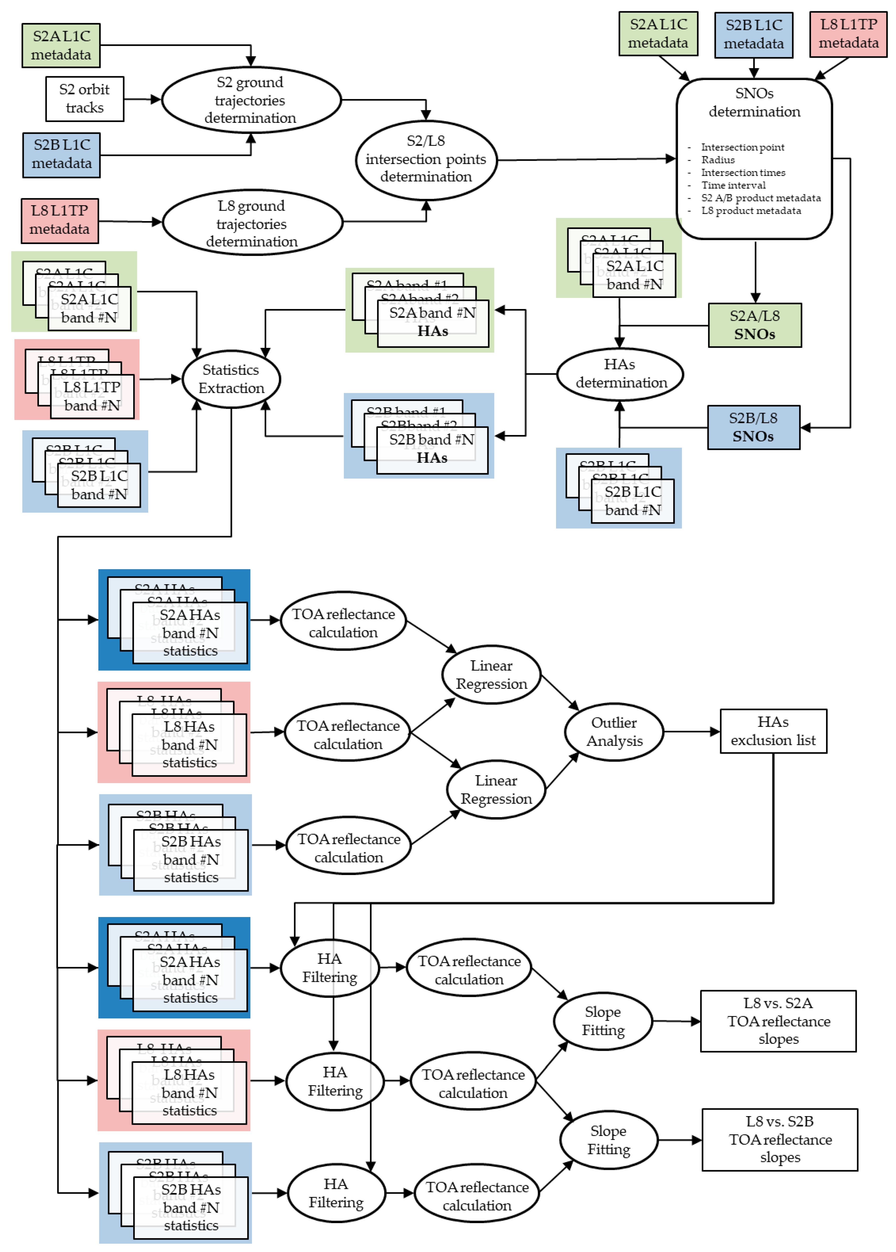
2.2. Ground Trajectory Determination and SNOs Finding
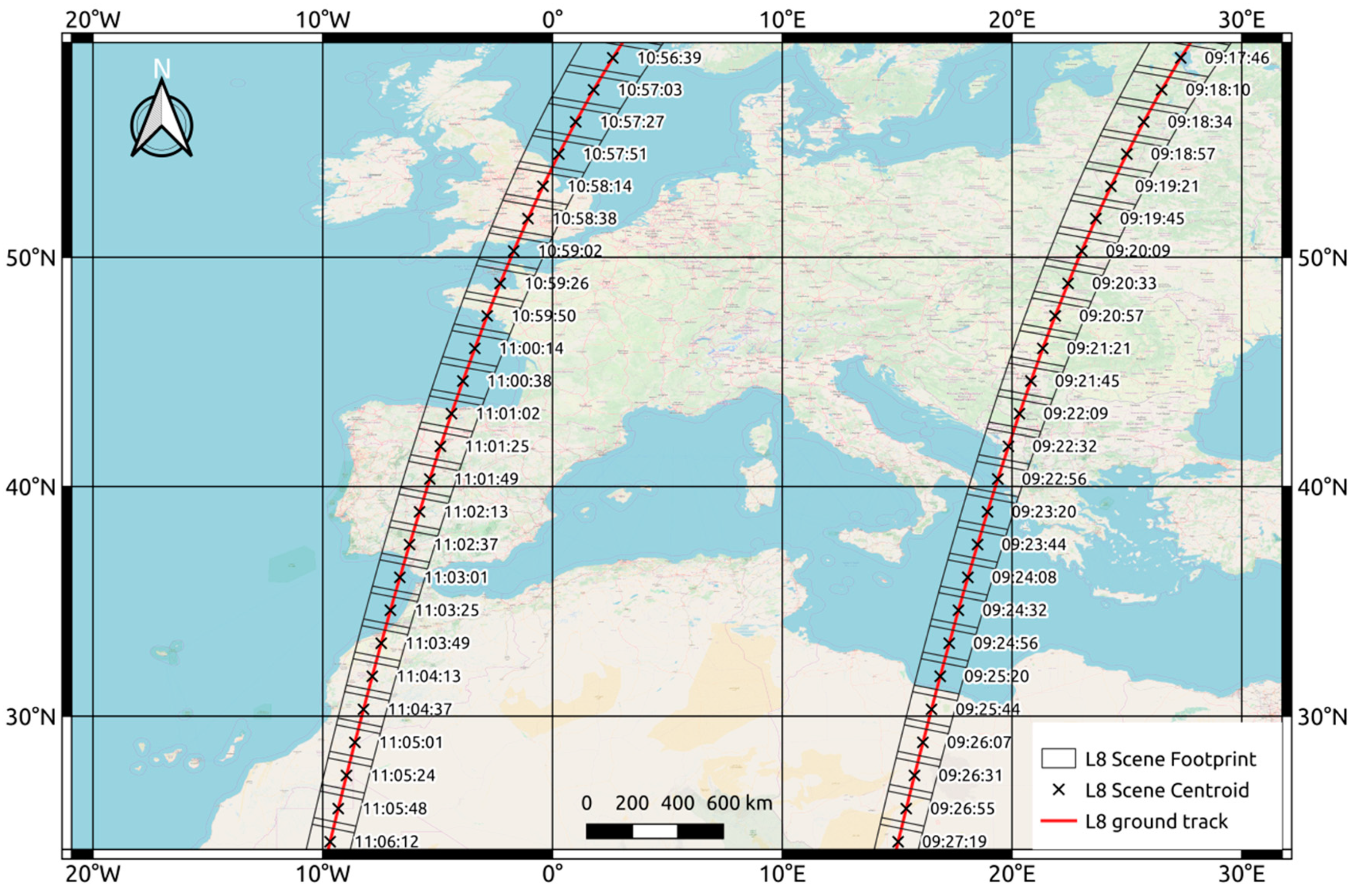
2.2.1. Landsat 8 Ground Trajectories
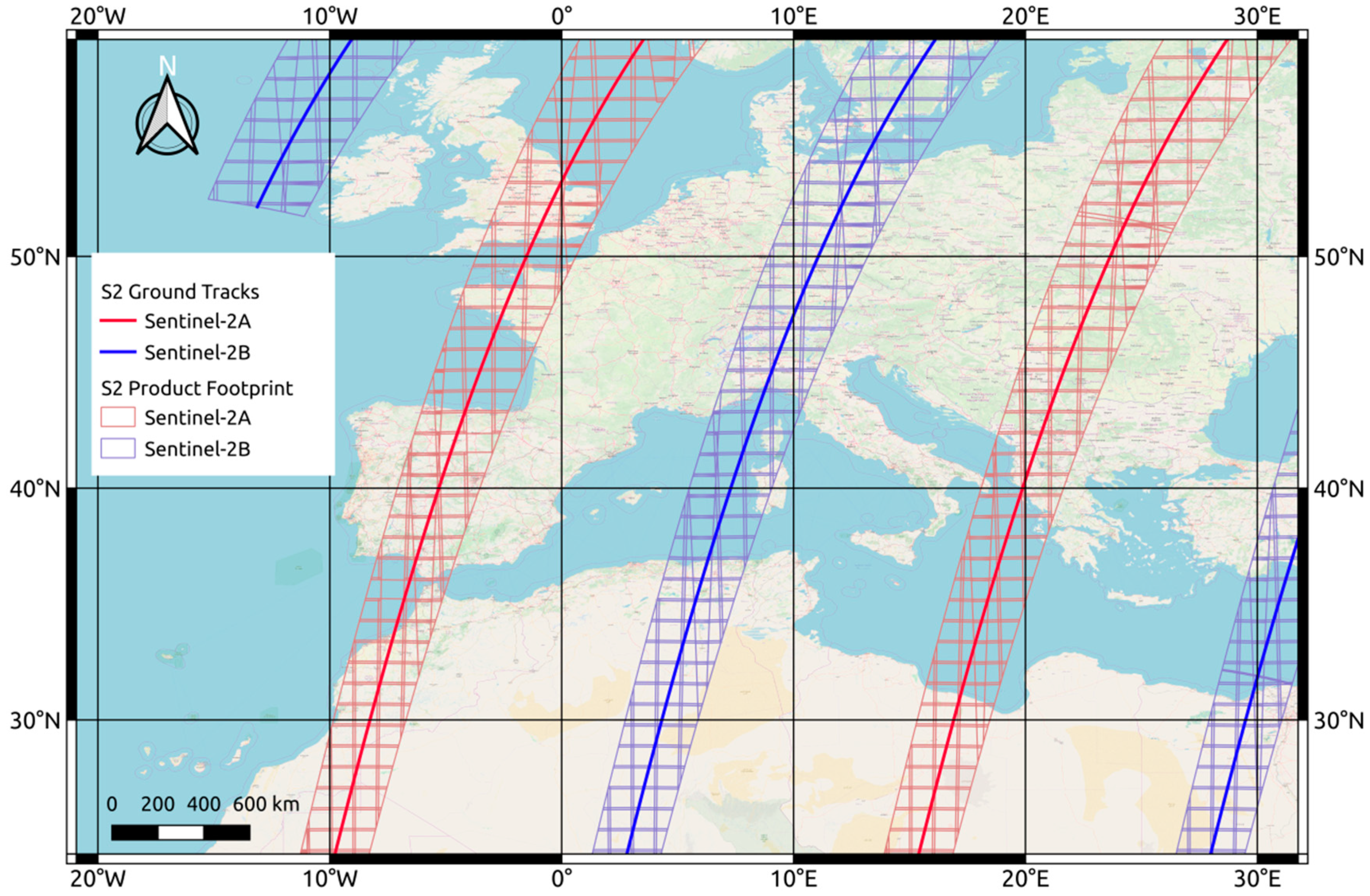
2.2.2. Sentinel-2 Ground Trajectories
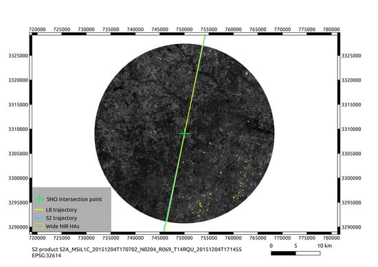
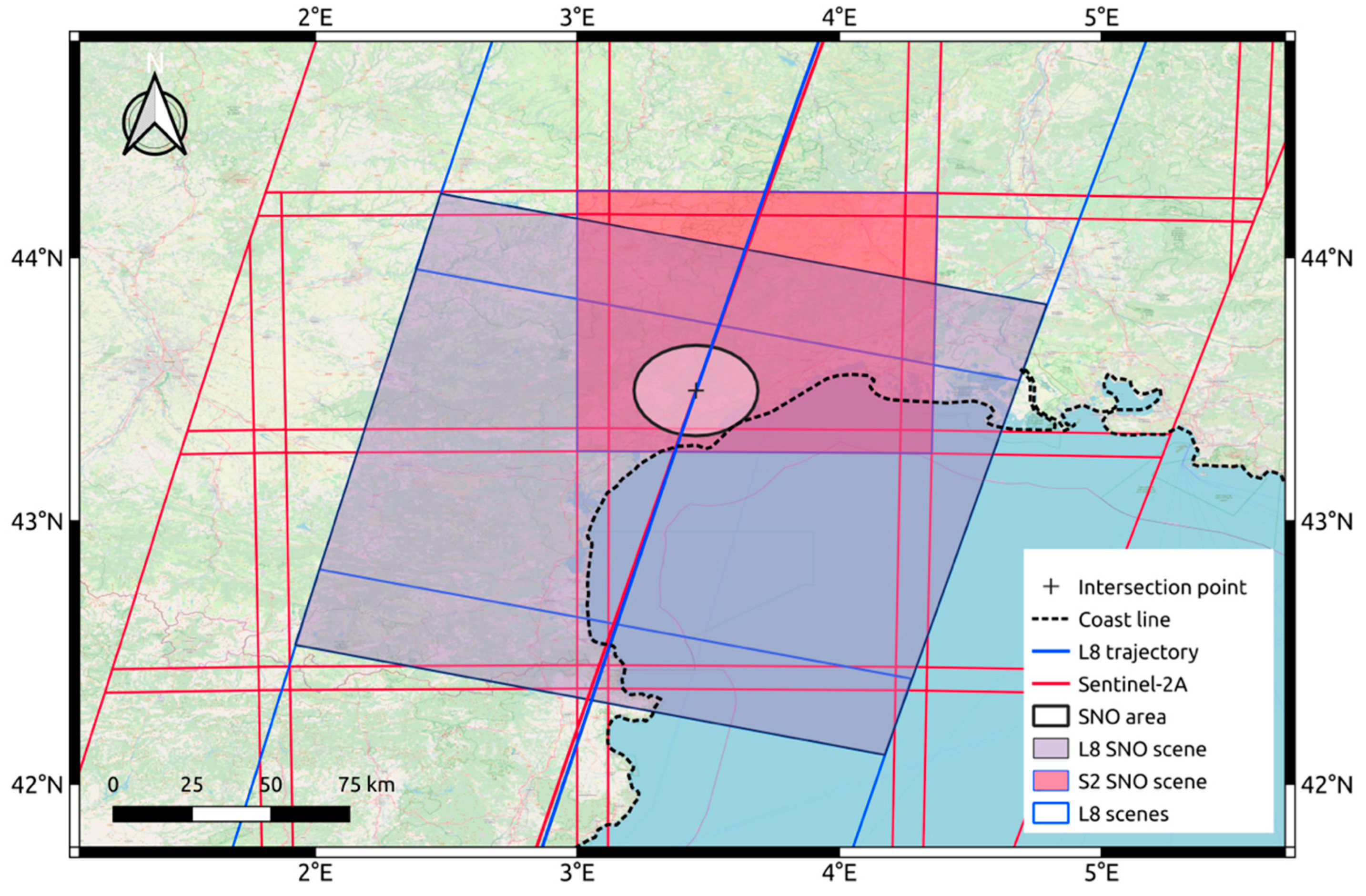
2.2.3. SNOs Determination
2.3. Statistics Extraction
2.3.1. Homogeneous Areas Creation
2.3.2. Statistics Retrieval
2.4. Data Analysis
3. Results
3.1. Data Analysis Remarks
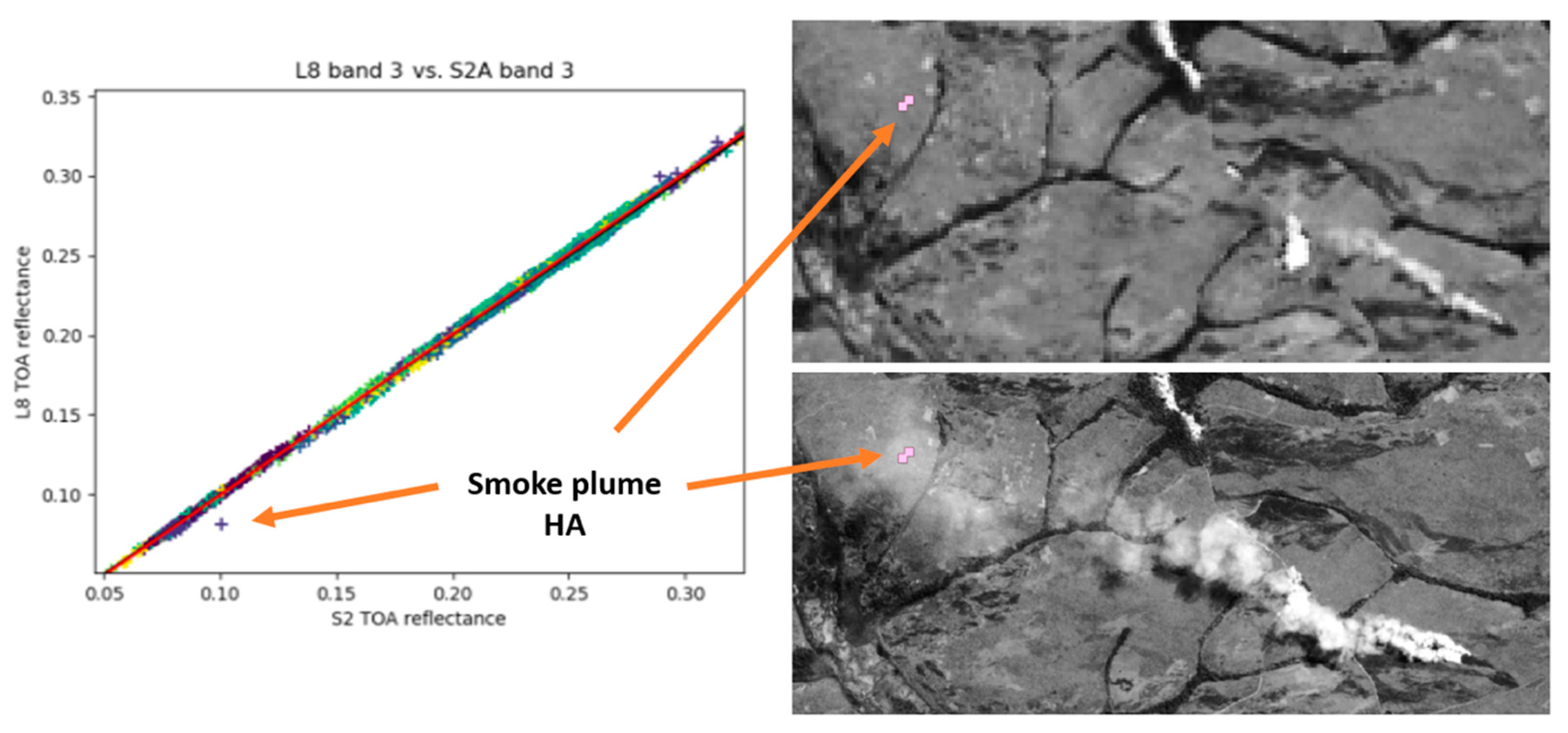
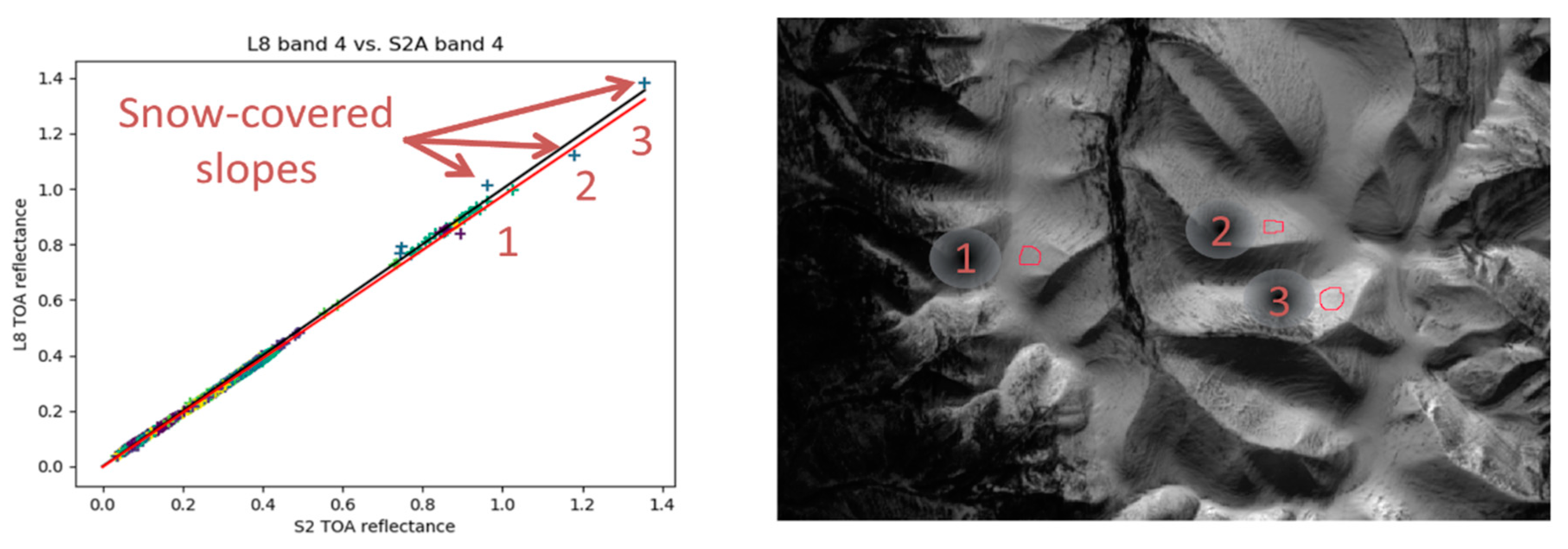
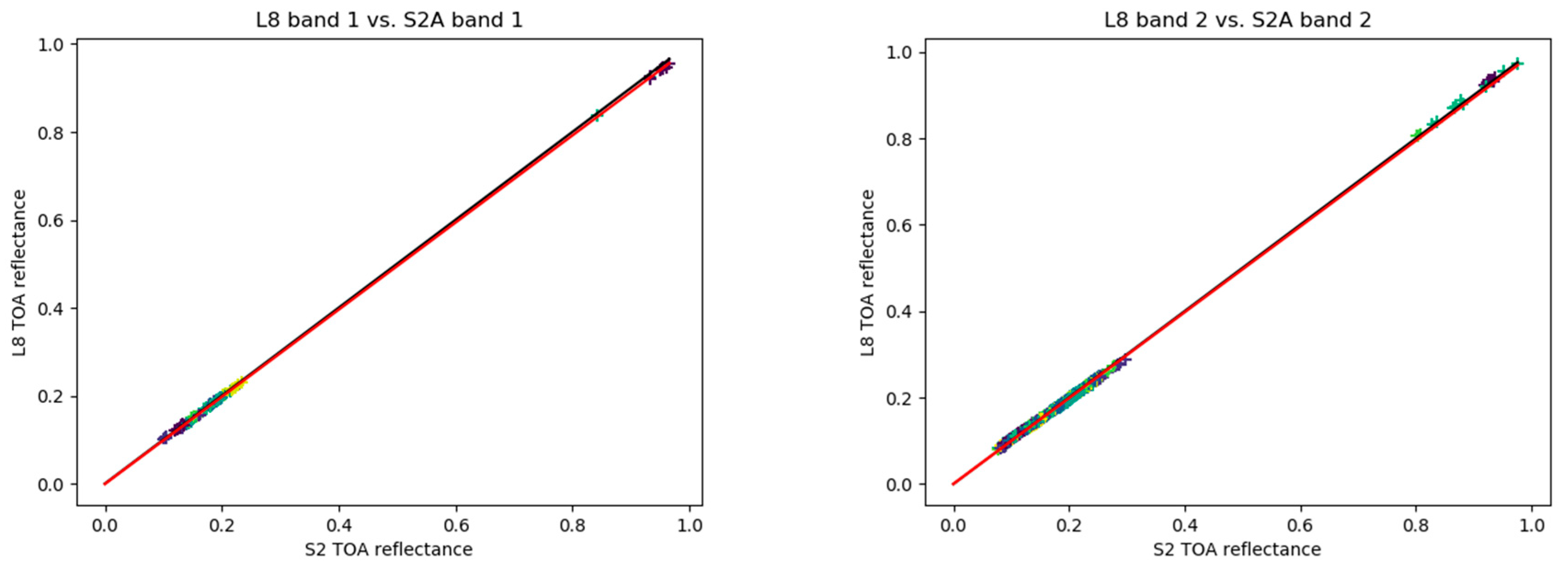
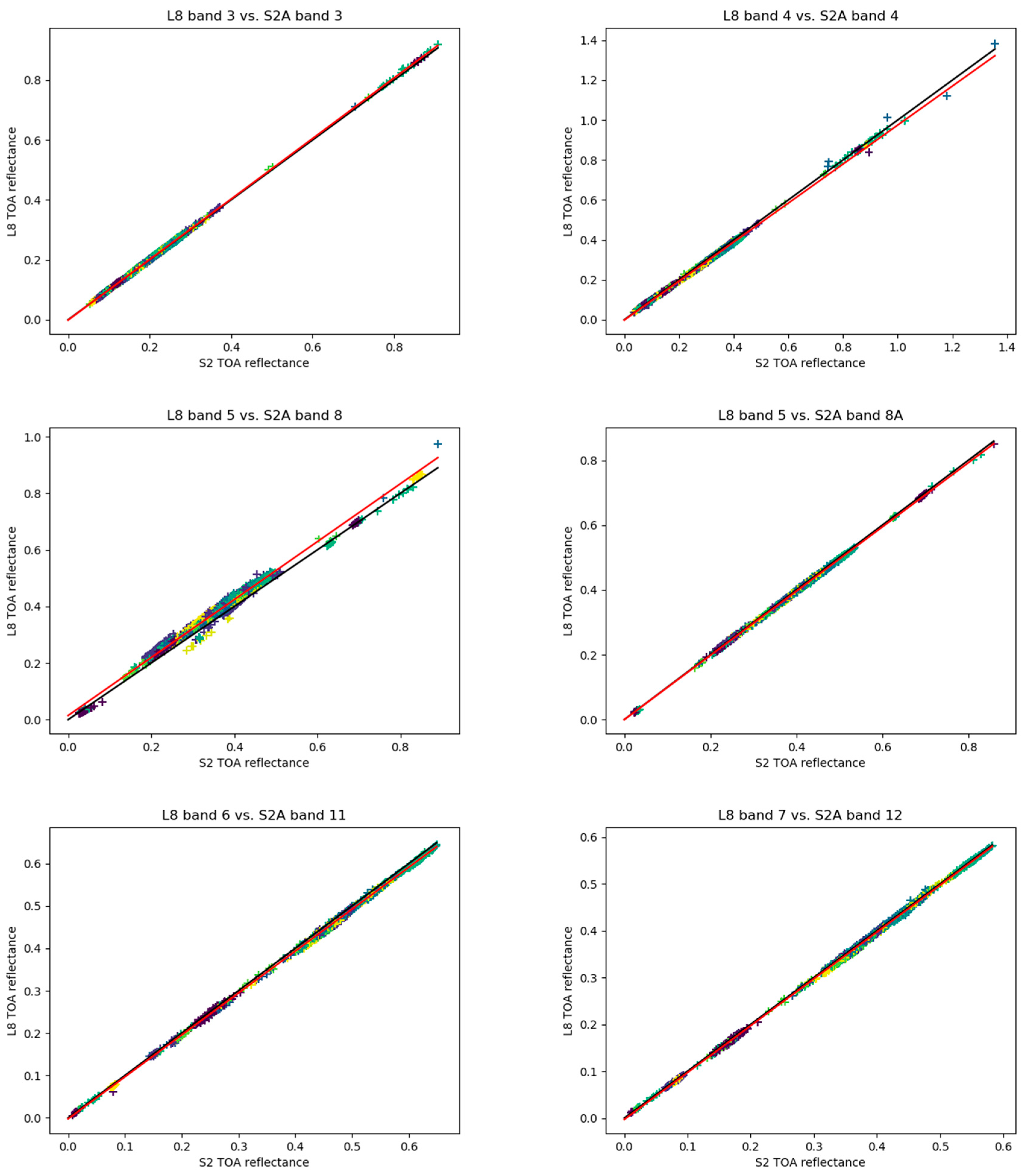
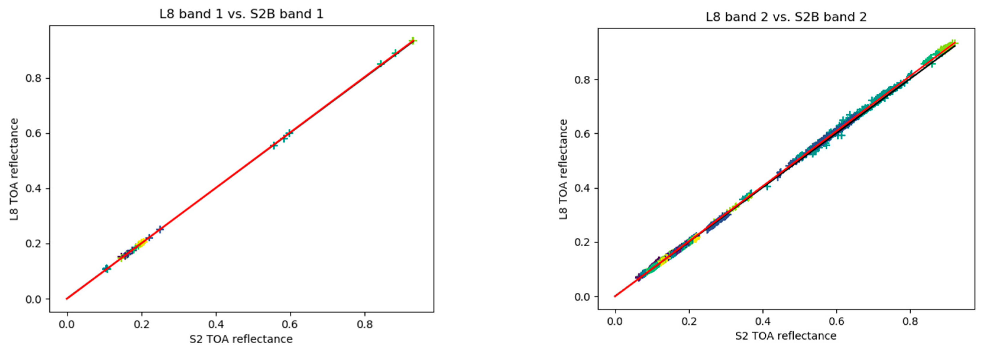
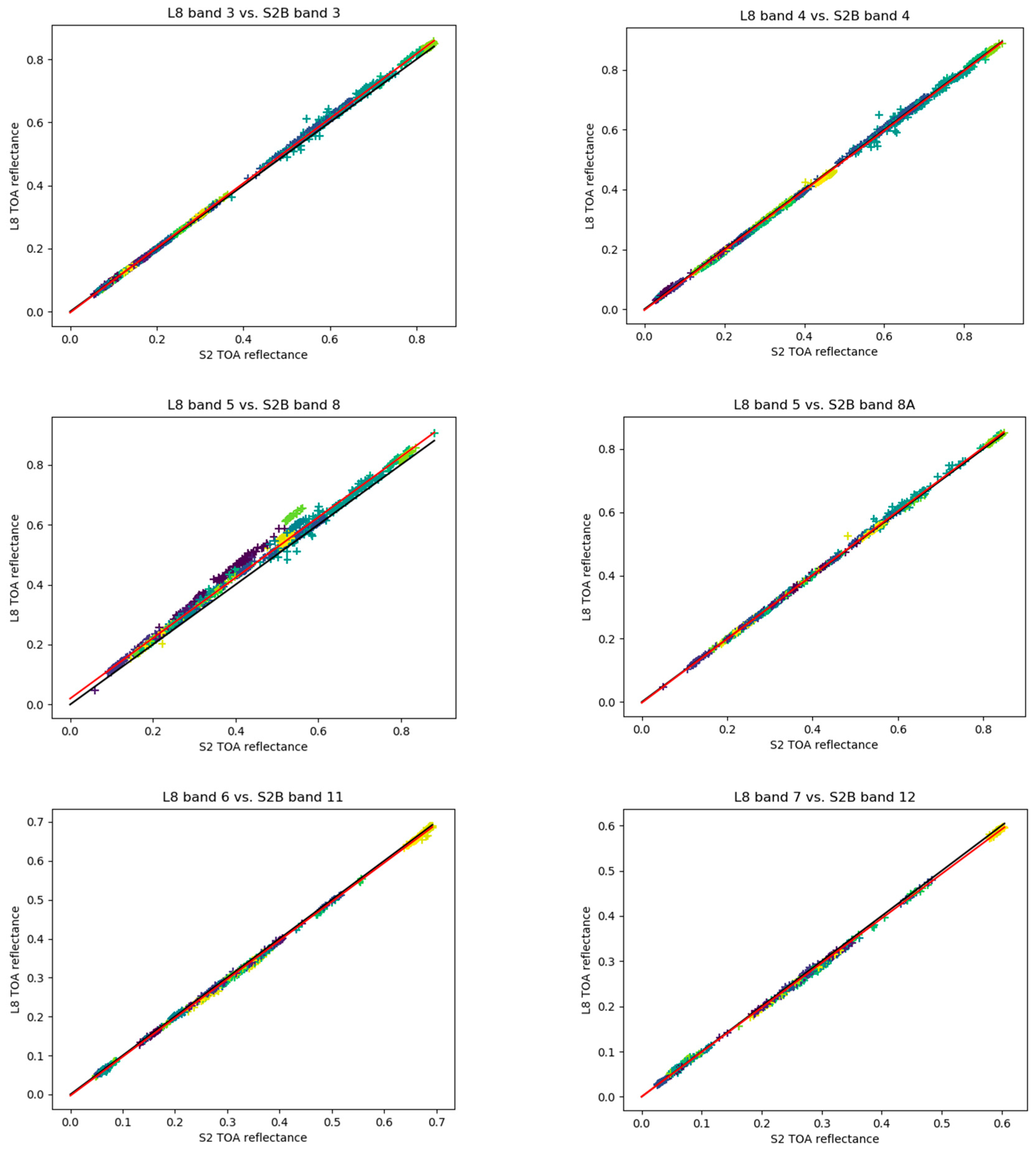
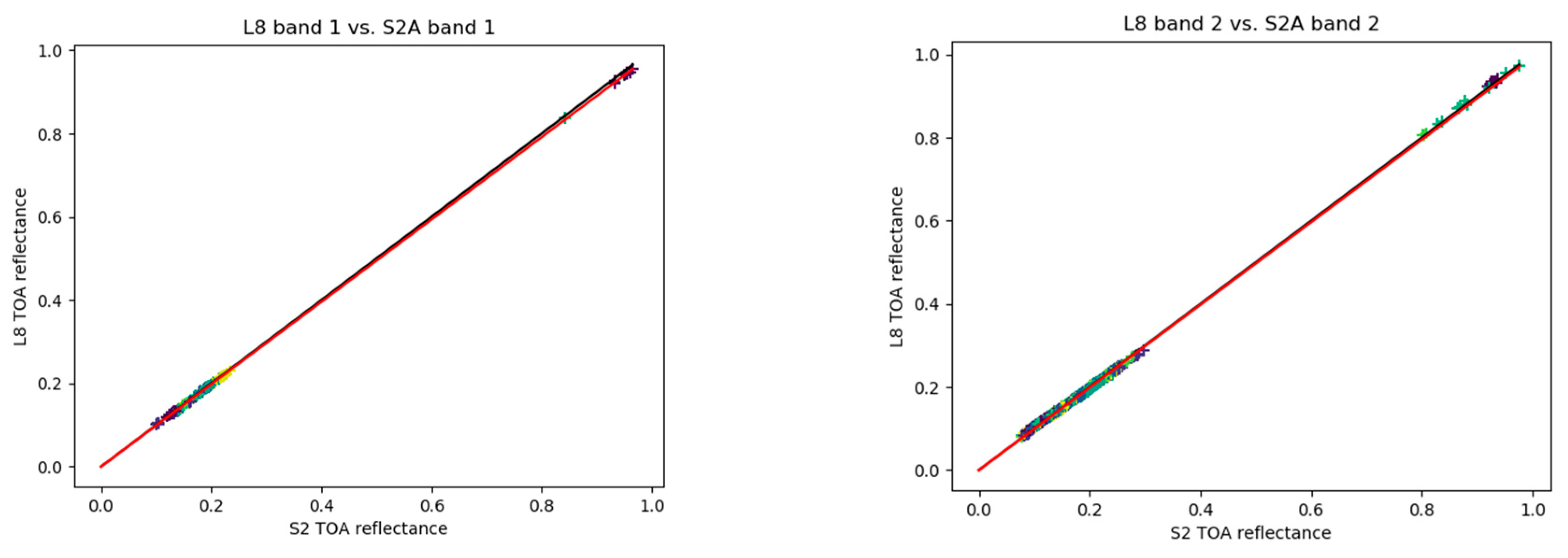
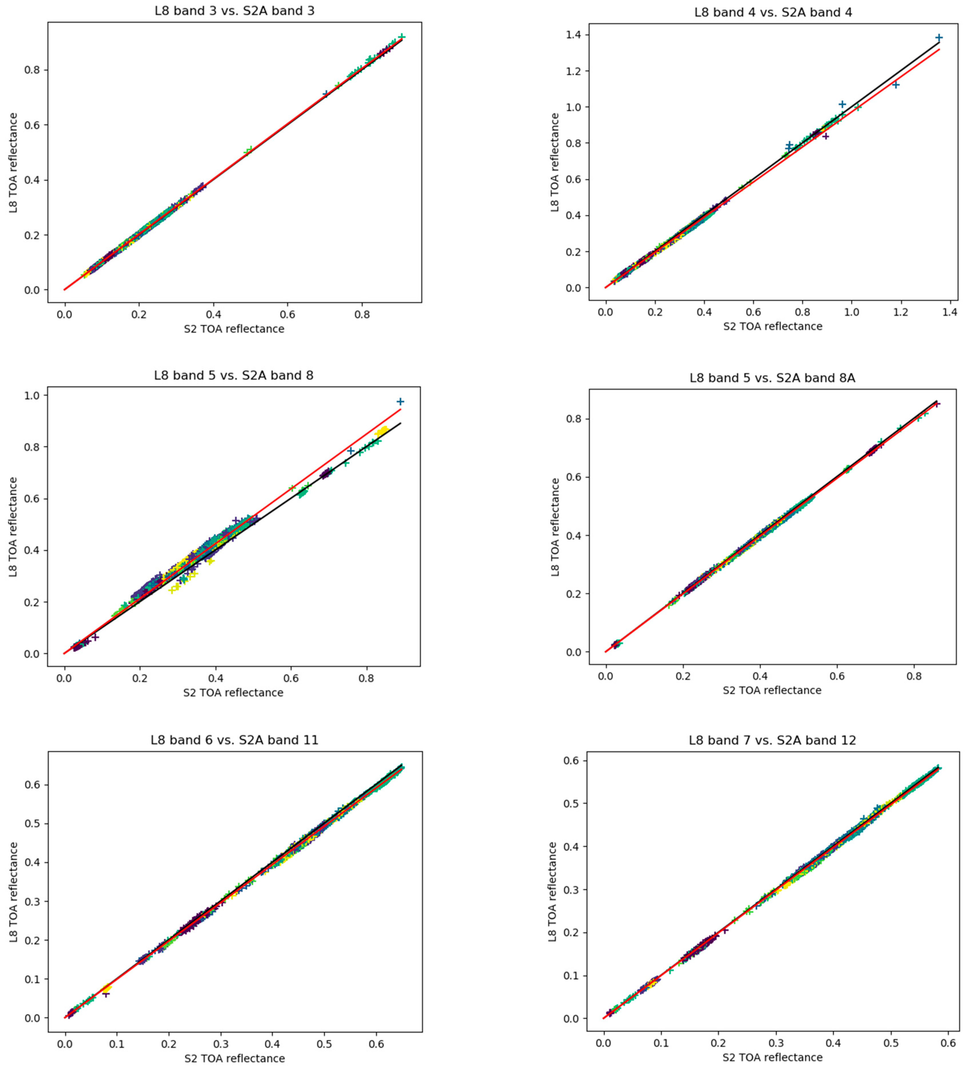
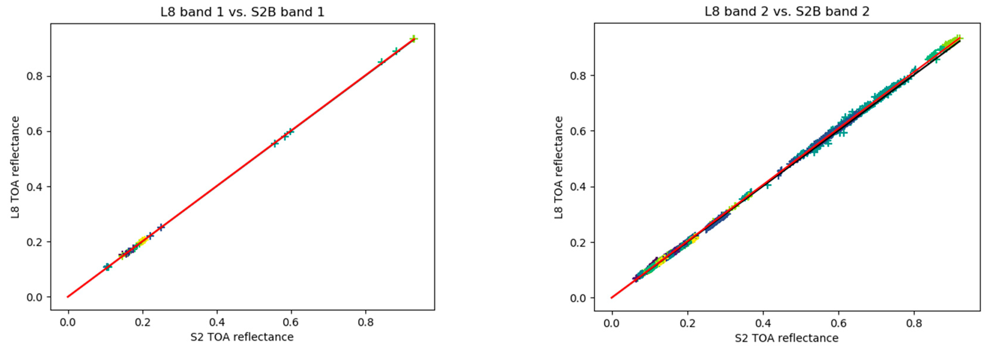
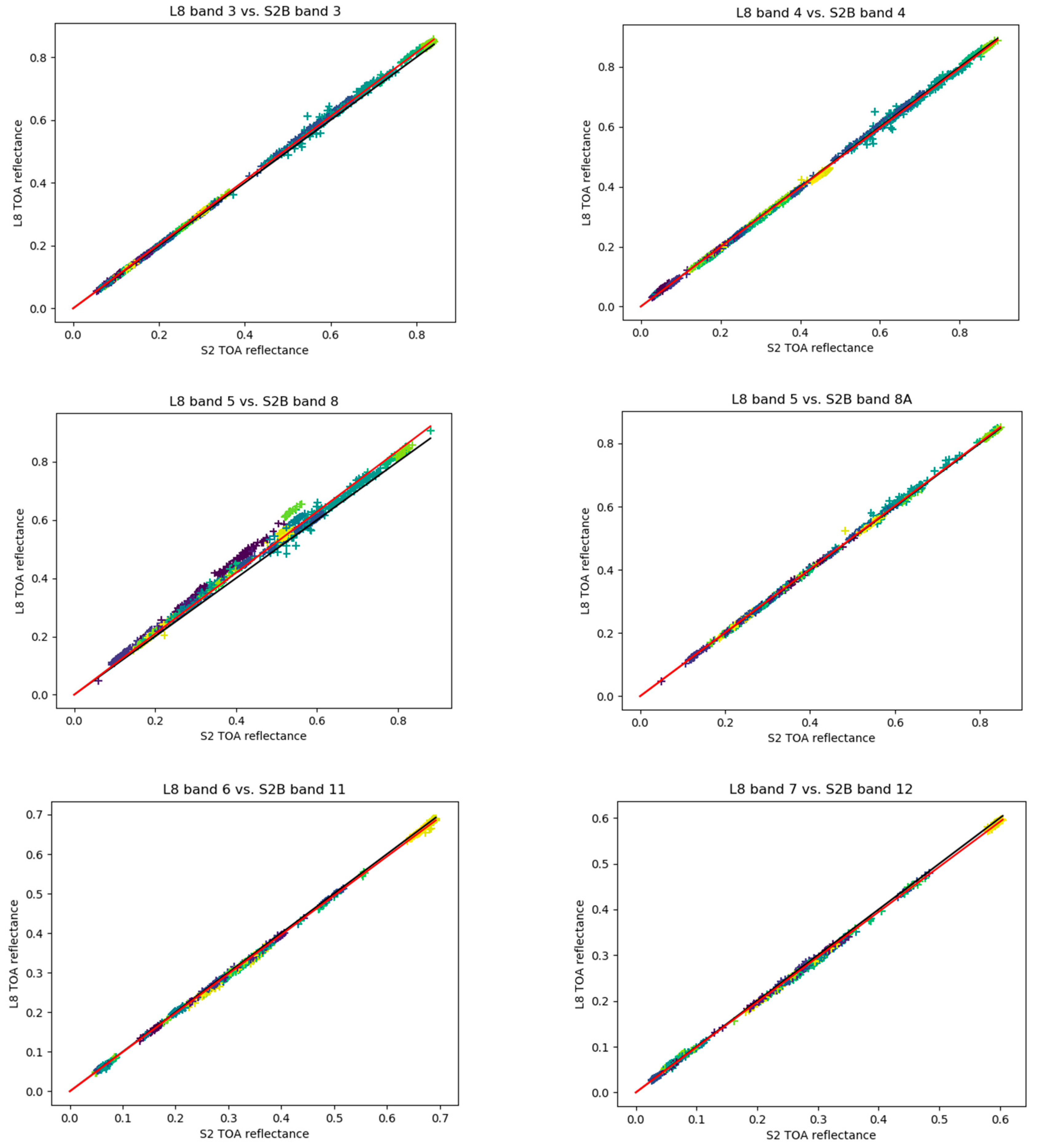
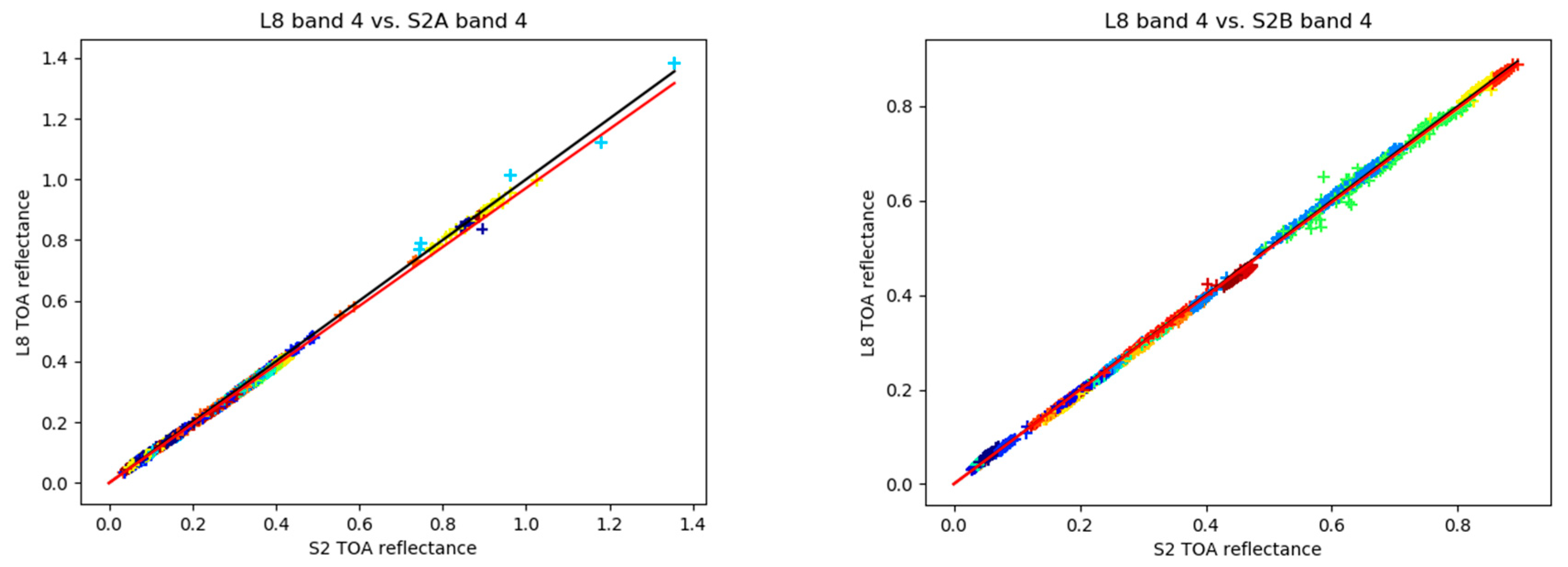
3.2. Correlation with TOA Reflectances
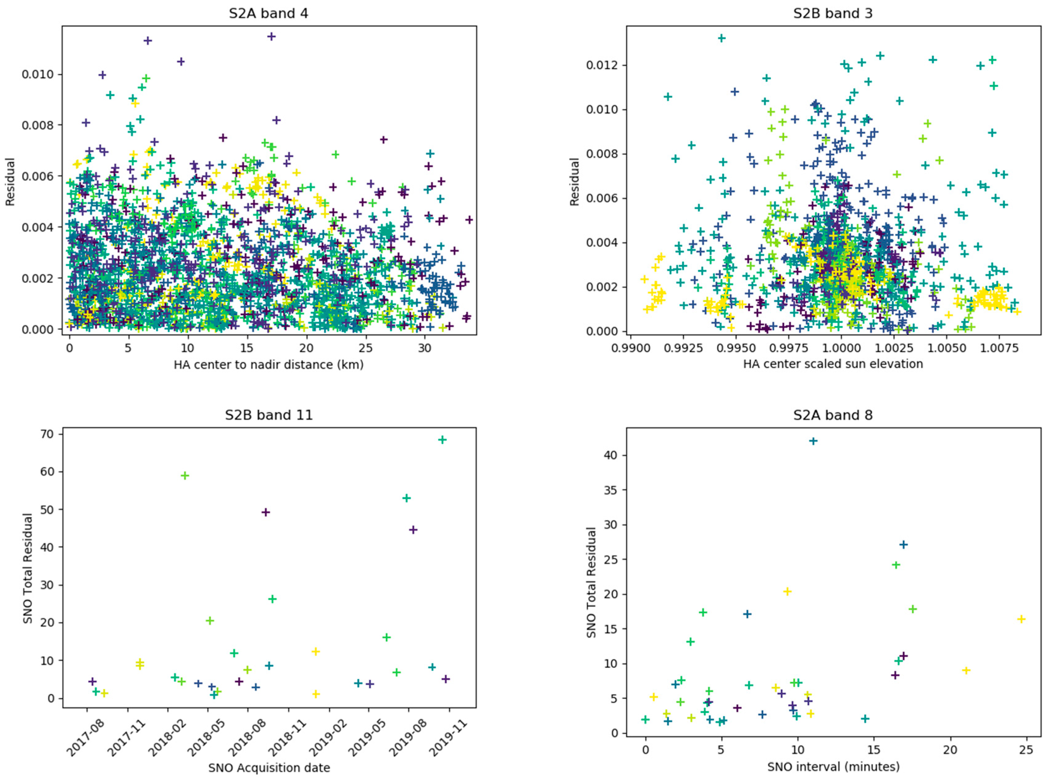
3.3. Dependence from Other Variables
- Average reflectance;
- Reflectance standard deviation;
- Solar elevation at the HA centroid;
- Solar azimuth at the HA centroid;
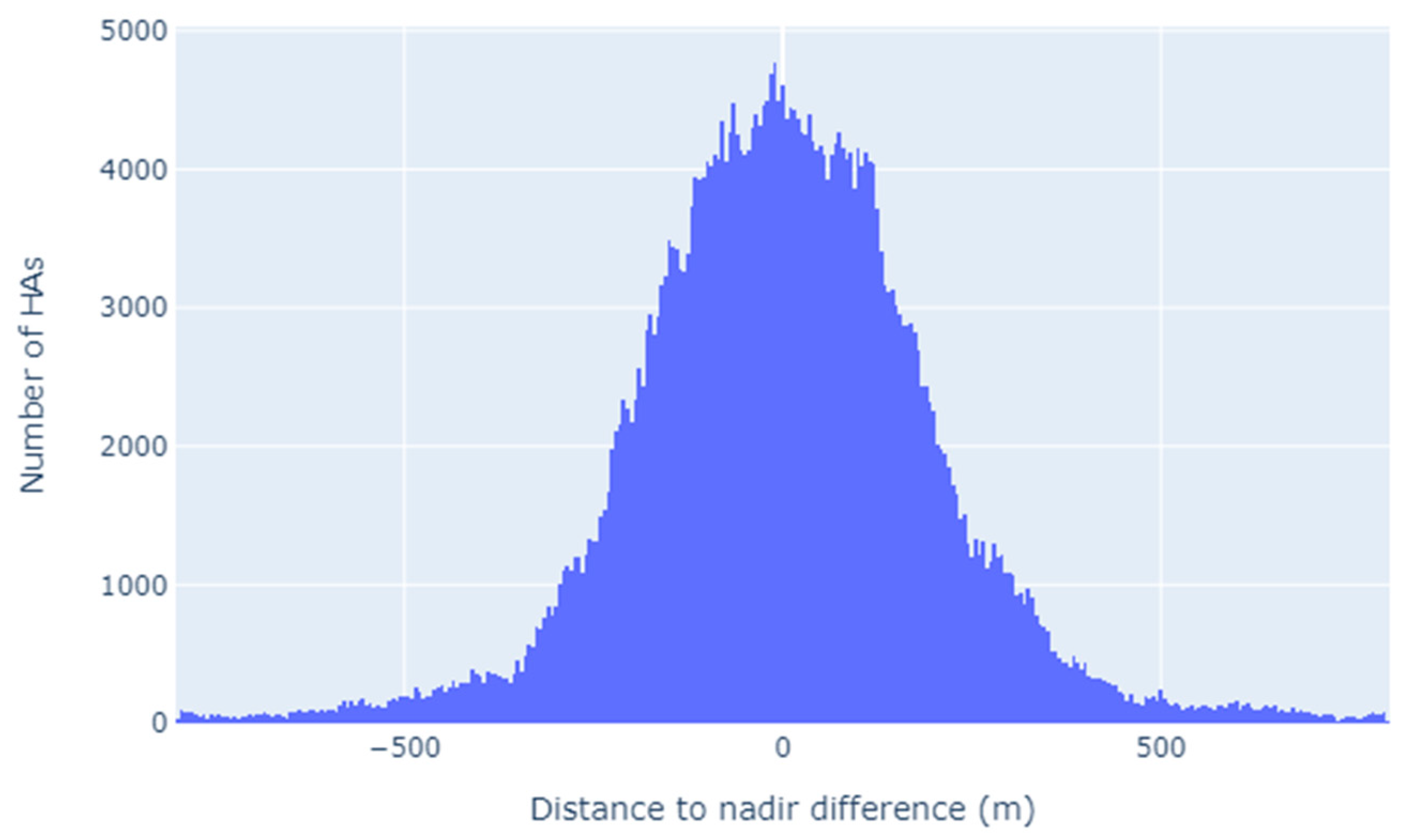
- HA centroid distance to nadir;
- HA latitude.
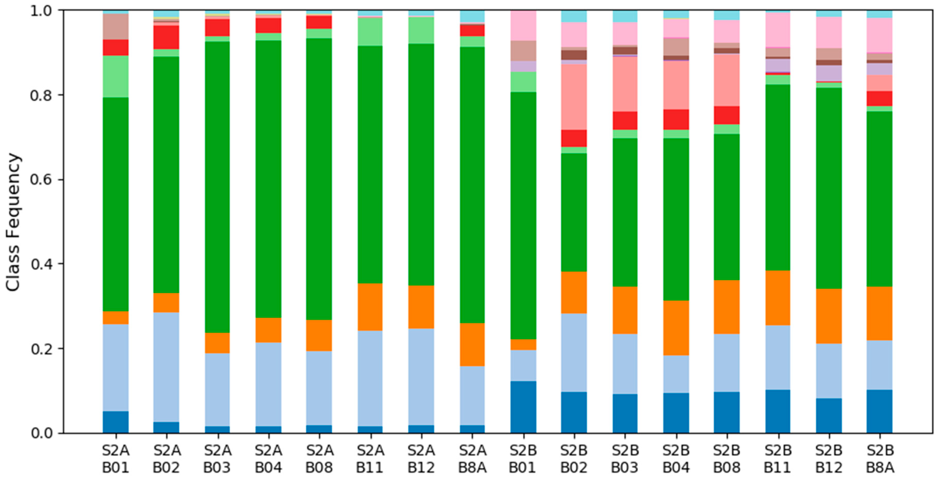
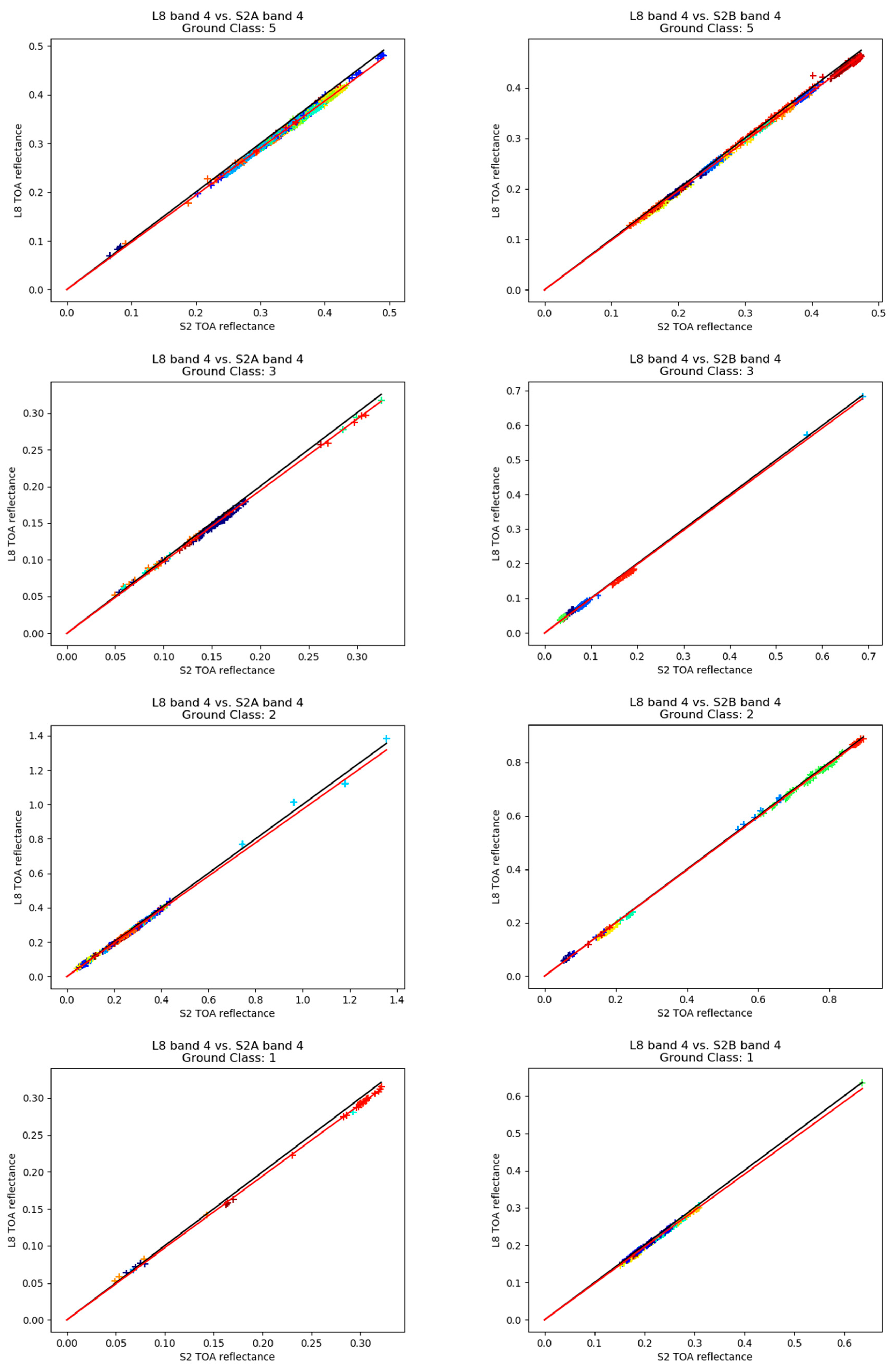
3.4. Ground Classes Distribution
- Derived from PROBA-V satellite observations for the 2015 reference year;
- Discrete classification with 23 classes;
- 100 m spatial resolution;
- An overall 80% accuracy.
4. Discussion
5. Conclusions
Author Contributions
Funding
Conflicts of Interest
Appendix A


Appendix B

| Acquisition Date | Sentinel Product Identifier | Landsat Product Identifier | SNO Intersection Lon, Lat (°) |
|---|---|---|---|
| 2015-08-12 | S2A_MSIL1C_20150812T104026_N0204_R008_T31TEJ_20150812T104021 | LC08_L1TP_197030_20150812_20170406_01_T1 | 3.4687, 43.5385 |
| 2015-09-04 | S2A_MSIL1C_20150904T072816_N0204_R049_T39UXP_20150904T073107 | LC08_L1TP_166027_20150904_20170404_01_T1 | 52.9557, 47.8579 |
| 2015-11-15 | S2A_MSIL1C_20151115T163532_N0204_R083_T16TGQ_20151115T163534 | LC08_L1TP_021029_20151115_20170225_01_T1 | −84.1691, 44.8334 |
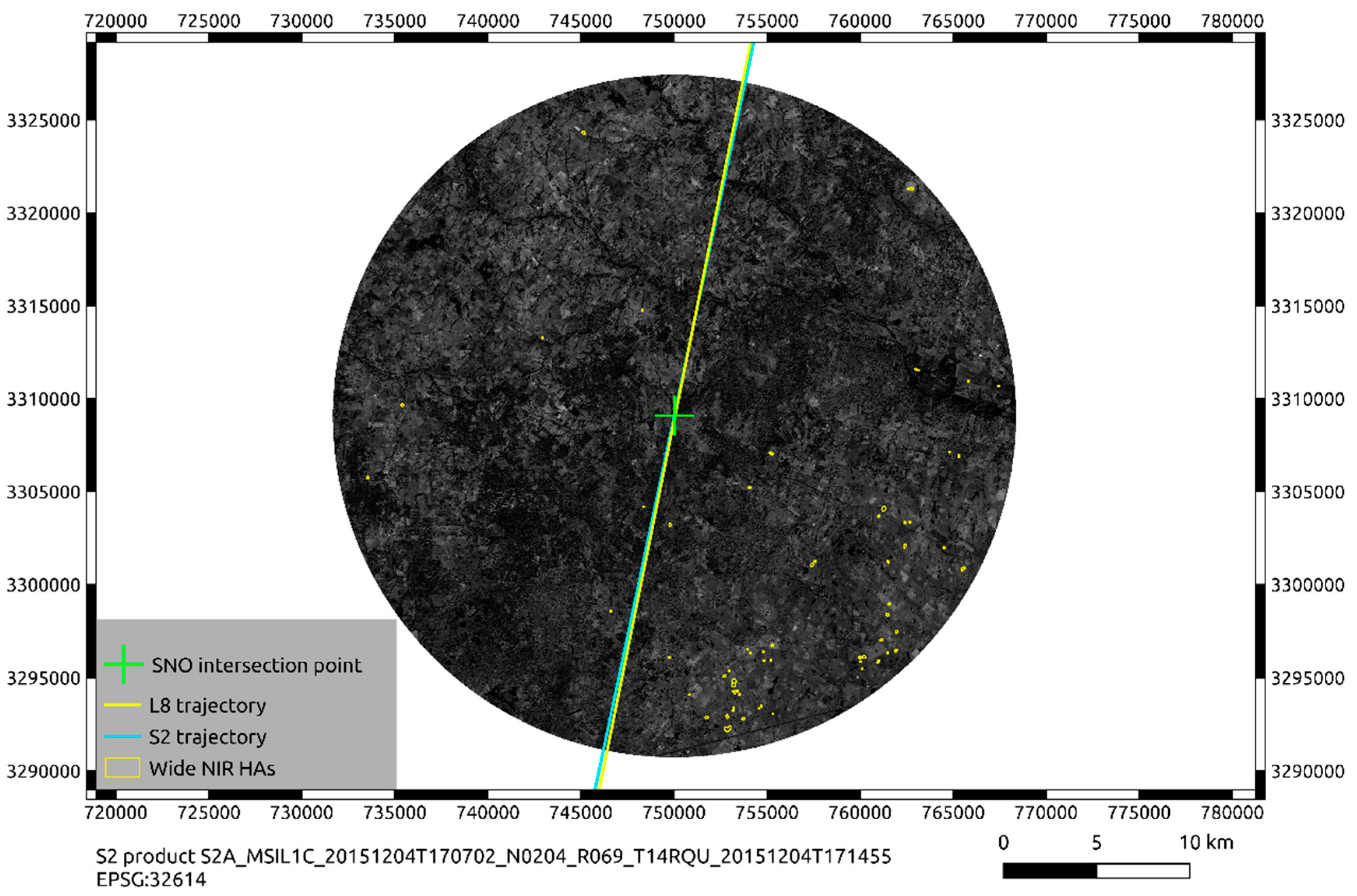
| 2015-12-04 | S2A_MSIL1C_20151204T170702_N0204_R069_T14RQU_20151204T171455 | LC08_L1TP_026039_20151204_20170224_01_T1 | −96.4111, 29.8870 |
| 2016-01-23 | S2A_MSIL1C_20160123T052112_N0201_R062_T43QGC_20160123T052434 | LC08_L1TP_145046_20160123_20170405_01_T1 | 77.3742, 20.3053 |
| 2016-02-07 | S2A_MSIL1C_20160207T112012_N0201_R137_T29RMJ_20160207T112209 | LC08_L1TP_202042_20160207_20170330_01_T1 | −9.4531, 25.4921 |
| 2016-03-28 | S2A_MSIL1C_20160328T060612_N0201_R134_T47XNE_20160328T060634 | LC08_L1TP_152006_20160328_20170327_01_T1 | 102.5021, 75.9571 |
| 2016-04-23 | S2A_MSIL1C_20160423T163322_N0201_R083_T16TFN_20160423T163610 | LC08_L1TP_021030_20160423_20170223_01_T1 | −84.9030, 42.8084 |
| 2016-05-05 | S2A_MSIL1C_20160505T004712_N0202_R102_T54HTK_20160505T004953 | LC08_L1TP_098082_20160505_20170325_01_T1 | 138.1499, −31.9755 |
| 2016-05-16 | S2A_MSIL1C_20160516T145922_N0202_R125_T22WFU_20160516T150205 | LC08_L1TP_006013_20160516_20170324_01_T1 | −48.4028, 66.4414 |
| 2016-06-08 | S2A_MSIL1C_20160608T101032_N0202_R022_T33UWV_20160608T101220 | LC08_L1TP_192023_20160608_20170324_01_T1 | 15.4202, 53.8655 |
| 2016-06-23 | S2A_MSIL1C_20160623T142012_N0204_R096_T26XMG_20160623T142007 | LC08_L1TP_233008_20160623_20170323_01_T1 | −28.0386, 73.2500 |
| 2016-06-27 | S2A_MSIL1C_20160627T085602_N0204_R007_T33MWM_20160627T091503 | LC08_L1TP_181066_20160627_20170323_01_T1 | 15.5755, −8.1661 |
| 2016-08-04 | S2A_MSIL1C_20160804T145922_N0204_R125_T22WFU_20160804T145917 | LC08_L1TP_006013_20160804_20170322_01_T1 | −48.1918, 66.6366 |
| 2016-08-27 | S2A_MSIL1C_20160827T101022_N0204_R022_T33UWV_20160827T101025 | LC08_L1TP_192023_20160827_20170321_01_T1 | 15.2991, 53.6280 |
| 2016-09-04 | S2A_MSIL1C_20160904T024542_N0204_R132_T53WNR_20160904T024545 | LC08_L1TP_120012_20160904_20170321_01_T1 | 137.3442, 68.1469 |
| 2016-10-12 | S2A_MSIL1C_20161012T004702_N0204_R102_T54JUR_20161012T004954 | LC08_L1TP_098079_20161012_20170319_01_T1 | 139.5657, −26.7139 |
| 2016-11-15 | S2A_MSIL1C_20161115T083222_N0204_R021_T35PNP_20161115T084140 | LC08_L1TP_176051_20161115_20170318_01_T1 | 27.7421, 12.6077 |
| 2016-12-08 | S2A_MSIL1C_20161208T052212_N0204_R062_T43QGC_20161208T052504 | LC08_L1TP_145046_20161208_20170317_01_T1 | 77.2887, 19.9503 |
| 2016-12-08 | S2A_MSIL1C_20161208T070252_N0204_R063_T41UNB_20161208T070254 | LC08_L1TP_161021_20161208_20170317_01_T1 | 63.9491, 55.1862 |
| 2016-12-19 | S2A_MSIL1C_20161219T163702_N0204_R083_T16TGQ_20161219T163834 | LC08_L1TP_021029_20161219_20170218_01_T1 | −84.3506, 44.3429 |
| 2017-01-07 | S2A_MSIL1C_20170107T170701_N0204_R069_T14RQT_20170107T170831 | LC08_L1TP_026040_20170107_20170218_01_T1 | −96.6369, 29.0480 |
| 2017-02-07 | S2A_MSIL1C_20170207T063021_N0204_R077_T43VEJ_20170207T063023 | LC08_L1TP_156017_20170207_20170216_01_T1 | 75.5459, 61.5073 |
| 2017-02-11 | S2A_MSIL1C_20170211T024831_N0204_R132_T53WNQ_20170211T024828 | LC08_L1TP_120013_20170211_20170217_01_T1 | 136.3952, 67.3552 |
| 2017-03-13 | S2A_MSIL1C_20170313T110831_N0204_R137_T29RMJ_20170313T111212 | LC08_L1TP_202042_20170313_20170328_01_T1 | −9.4439, 25.5280 |
| 2017-03-28 | S2A_MSIL1C_20170328T170301_N0204_R069_T14RQT_20170328T170619 | LC08_L1TP_026040_20170328_20170414_01_T1 | −96.5164, 29.4971 |
| 2017-04-05 | S2A_MSIL1C_20170405T075611_N0204_R035_T37REQ_20170405T081035 | LC08_L1TP_171038_20170405_20170414_01_T1 | 39.9037, 31.2414 |
| 2017-04-24 | S2A_MSIL1C_20170424T082601_N0204_R021_T35PNP_20170424T083830 | LC08_L1TP_176051_20170424_20170502_01_T1 | 27.6998, 12.4221 |
| 2017-05-13 | S2A_MSIL1C_20170513T090021_N0205_R007_T33MWM_20170513T092026 | LC08_L1TP_181065_20170513_20170525_01_T1 | 15.6498, −7.8332 |
| 2017-06-01 | S2A_MSIL1C_20170601T110651_N0205_R137_T29RMJ_20170601T111225 | LC08_L1TP_202042_20170601_20170615_01_T1 | −9.3525, 25.8857 |
| 2017-06-09 | S2A_MSIL1C_20170609T004711_N0205_R102_T54JUQ_20170609T005308 | LC08_L1TP_098079_20170609_20170616_01_T1 | 139.3032, −27.7203 |
| 2017-06-24 | S2A_MSIL1C_20170624T075611_N0205_R035_T37SFS_20170624T075954 | LC08_L1TP_171037_20170624_20170701_01_T1 | 40.3766, 32.9272 |
| 2017-07-13 | S2A_MSIL1C_20170713T150911_N0205_R025_T25XEF_20170713T150911 | LC08_L1TP_007005_20170713_20170726_01_T1 | −31.3113, 76.5751 |
| 2017-07-15 | S2B_MSIL1C_20170715T081609_N0205_R121_T38VNL_20170715T081603 | LC08_L1TP_174019_20170715_20170727_01_T1 | 46.2853, 59.3029 |
| 2017-07-28 | S2A_MSIL1C_20170728T155901_N0205_R097_T22XDG_20170728T160023 | LC08_L1TP_016008_20170728_20170810_01_T1 | −52.9801, 73.3561 |
| 2017-08-01 | S2A_MSIL1C_20170801T140021_N0205_R010_T26WNE_20170801T140016 | LC08_L1TP_229009_20170801_20170811_01_T1 | −25.5732, 71.9617 |
| 2017-08-14 | S2B_MSIL1C_20170814T183309_N0205_R127_T11SPV_20170814T183307 | LC08_L1TP_039035_20170814_20170825_01_T1 | −114.9258, 35.6075 |
| 2017-08-20 | S2A_MSIL1C_20170820T160901_N0205_R140_T22XDH_20170820T160902 | LC08_L1TP_017007_20170820_20170826_01_T1 | −53.0172, 74.4073 |
| 2017-08-20 | S2A_MSIL1C_20170820T110651_N0205_R137_T29RMJ_20170820T111220 | LC08_L1TP_202042_20170820_20170826_01_T1 | −9.2816, 26.1619 |
| 2017-08-22 | S2B_MSIL1C_20170822T141949_N0205_R096_T27XVD_20170822T141947 | LC08_L1TP_232007_20170822_20170911_01_T1 | −22.9999, 75.2631 |
| 2017-08-28 | S2A_MSIL1C_20170828T004711_N0205_R102_T54JUR_20170828T005307 | LC08_L1TP_098078_20170828_20170914_01_T1 | 139.6069, −26.5550 |
| 2017-09-04 | S2A_MSIL1C_20170904T165851_N0205_R069_T14RQV_20170904T170402 | LC08_L1TP_026039_20170904_20180125_01_T1 | −96.1340, 30.9020 |
| 2017-09-10 | S2B_MSIL1C_20170910T095019_N0205_R079_T32QNJ_20170910T100356 | LC08_L1TP_189045_20170910_20170927_01_T1 | 9.5894, 21.0792 |
| 2017-09-12 | S2A_MSIL1C_20170912T075611_N0205_R035_T37SFT_20170912T075950 | LC08_L1TP_171037_20170912_20170928_01_T1 | 40.6307, 33.8132 |
| 2017-09-20 | S2A_MSIL1C_20170920T021601_N0205_R003_T55WEU_20170920T021627 | LC08_L1TP_115010_20170920_20170930_01_T1 | 148.6628, 70.8084 |
| 2017-09-25 | S2B_MSIL1C_20170925T142029_N0205_R010_T20JKN_20170925T142023 | LC08_L1TP_230081_20170925_20180528_01_T1 | −65.1780, −29.8396 |
| 2017-10-20 | S2A_MSIL1C_20171020T090021_N0205_R007_T33LVH_20171020T091816 | LC08_L1TP_181068_20171020_20171106_01_T1 | 14.9176, −11.0946 |
| 2017-10-22 | S2B_MSIL1C_20171022T071249_N0205_R106_T38NPK_20171022T072130 | LC08_L1TP_163057_20171022_20171107_01_T1 | 45.9595, 4.0151 |
| 2017-11-08 | S2A_MSIL1C_20171108T111251_N0206_R137_T29QMG_20171108T145151 | LC08_L1TP_202043_20171108_20171121_01_T1 | −9.8014, 24.1148 |
| 2017-11-29 | S2B_MSIL1C_20171129T095339_N0206_R079_T32QNJ_20171129T115638 | LC08_L1TP_189046_20171129_20171207_01_T1 | 9.5698, 20.9984 |
| 2017-11-29 | S2B_MSIL1C_20171129T113419_N0206_R080_T30UVG_20171129T133534 | LC08_L1TP_205021_20171129_20171207_01_T1 | −3.7183, 55.7397 |
| 2017-11-29 | S2B_MSIL1C_20171129T081249_N0206_R078_T34HFK_20171129T115343 | LC08_L1TP_173082_20171129_20171207_01_T1 | 22.2712, −32.2408 |
| 2017-12-01 | S2A_MSIL1C_20171201T080301_N0206_R035_T37SFS_20171201T100357 | LC08_L1TP_171037_20171201_20171207_01_T1 | 40.4777, 33.2813 |
| 2018-01-27 | S2A_MSIL1C_20180127T111321_N0206_R137_T29RMK_20180127T162747 | LC08_L1TP_202042_20180127_20180207_01_T1 | −9.1689, 26.5989 |
| 2018-01-29 | S2B_MSIL1C_20180129T092229_N0206_R093_T34SEH_20180129T112249 | LC08_L1TP_184034_20180129_20180207_01_T1 | 21.7305, 37.9342 |
| 2018-02-17 | S2B_MSIL1C_20180217T081009_N0206_R078_T34JFL_20180217T121107 | LC08_L1TP_173082_20180217_20180307_01_T1 | 22.5676, −31.1783 |
| 2018-03-04 | S2B_MSIL1C_20180304T142029_N0206_R010_T20JLR_20180304T191354 | LC08_L1TP_230079_20180304_20180319_01_T1 | −64.3401, −26.6743 |
| 2018-03-10 | S2A_MSIL1C_20180310T082751_N0206_R021_T35PPS_20180310T122012 | LC08_L1TP_176050_20180310_20180320_01_T1 | 28.2813, 14.9583 |
| 2018-03-12 | S2B_MSIL1C_20180312T063639_N0206_R120_T40RGR_20180312T102023 | LC08_L1TP_158041_20180312_20180320_01_T1 | 59.1391, 27.8870 |
| 2018-03-31 | S2B_MSIL1C_20180331T070619_N0206_R106_T38NPP_20180331T100829 | LC08_L1TP_163055_20180331_20180405_01_T1 | 46.7244, 7.4643 |
| 2018-04-02 | S2A_MSIL1C_20180402T051651_N0206_R062_T43QGD_20180402T090406 | LC08_L1TP_145046_20180402_20180416_01_T1 | 77.5245, 20.9270 |
| 2018-04-11 | S2B_MSIL1C_20180411T181919_N0206_R127_T11SPT_20180411T220513 | LC08_L1TP_039036_20180411_20180417_01_T1 | −115.3518, 34.1632 |
| 2018-04-17 | S2A_MSIL1C_20180417T110651_N0206_R137_T29RMH_20180417T164957 | LC08_L1TP_202043_20180417_20180501_01_T1 | −9.5650, 25.0522 |
| 2018-04-25 | S2A_MSIL1C_20180425T004711_N0206_R102_T54JUT_20180425T021141 | LC08_L1TP_098077_20180425_20180502_01_T1 | 140.0578, −24.7916 |
| 2018-05-08 | S2B_MSIL1C_20180508T080609_N0206_R078_T34HFK_20180508T133204 | LC08_L1TP_173082_20180508_20180517_01_T1 | 22.2174, −32.4317 |
| 2018-05-10 | S2A_MSIL1C_20180510T094031_N0206_R036_T35VME_20180510T114819 | LC08_L1TP_187019_20180510_20180517_01_T1 | 25.3924, 58.1392 |
| 2018-05-10 | S2A_MSIL1C_20180510T043701_N0206_R033_T50XNG_20180510T074003 | LC08_L1TP_139008_20180510_20180517_01_T1 | 117.6388, 73.0903 |
| 2018-05-12 | S2B_MSIL1C_20180512T074729_N0206_R135_T40VDP_20180512T113937 | LC08_L1TP_169017_20180512_20180517_01_T1 | 55.7179, 61.9131 |
| 2018-05-16 | S2B_MSIL1C_20180516T022549_N0206_R046_T52UFE_20180516T040424 | LC08_L1TP_117022_20180516_20180604_01_T1 | 131.2951, 54.0036 |
| 2018-05-16 | S2B_MSIL1C_20180516T040539_N0206_R047_T50WMV_20180516T070218 | LC08_L1TP_133013_20180516_20180604_01_T1 | 116.1178, 67.2360 |
| 2018-05-23 | S2B_MSIL1C_20180523T142039_N0206_R010_T20JLP_20180523T192205 | LC08_L1TP_230080_20180523_20180605_01_T1 | −64.8003, −28.4302 |
| 2018-05-23 | S2B_MSIL1C_20180523T204019_N0206_R014_T10XDG_20180524T001026 | LC08_L1TP_061008_20180523_20180605_01_T1 | −123.9418, 73.1388 |
| 2018-06-04 | S2B_MSIL1C_20180604T043659_N0206_R033_T48WXU_20180604T081821 | LC08_L1TP_138013_20180604_20180615_01_T1 | 107.7603, 66.5143 |
| 2018-06-06 | S2A_MSIL1C_20180606T024651_N0206_R132_T53WPS_20180606T040212 | LC08_L1TP_120011_20180606_20180615_01_T1 | 138.5057, 69.0425 |
| 2018-06-07 | S2B_MSIL1C_20180607T180919_N0206_R084_T17XMD_20180607T213729 | LC08_L1TP_038006_20180607_20180615_01_T1 | −80.8364, 75.2836 |
| 2018-06-11 | S2B_MSIL1C_20180611T174909_N0206_R141_T13UFR_20180611T213053 | LC08_L1TP_034025_20180611_20180615_01_T1 | −102.1482, 50.1601 |
| 2018-06-13 | S2A_MSIL1C_20180613T155901_N0206_R097_T19VCC_20180613T194300 | LC08_L1TP_016021_20180613_20180703_01_T1 | −71.3207, 56.3924 |
| 2018-06-23 | S2B_MSIL1C_20180623T020449_N0206_R017_T51KTT_20180623T033510 | LC08_L1TP_111074_20180623_20180703_01_T1 | 120.9584, −20.5823 |
| 2018-06-30 | S2B_MSIL1C_20180630T181919_N0206_R127_T11SQA_20180630T232219 | LC08_L1TP_039035_20180630_20180716_01_T1 | −114.5805, 36.7495 |
| 2018-07-02 | S2A_MSIL1C_20180702T150721_N0206_R082_T19MBT_20180702T195445 | LC08_L1TP_005062_20180702_20180716_01_T1 | −71.3037, −2.6055 |
| 2018-07-02 | S2A_MSIL1C_20180702T162901_N0206_R083_T16TGS_20180702T214026 | LC08_L1TP_021028_20180702_20180716_01_T1 | −83.6504, 46.1967 |
| 2018-07-10 | S2A_MSIL1C_20180710T072621_N0206_R049_T39UXP_20180710T085441 | LC08_L1TP_166027_20180710_20180717_01_T1 | 53.0450, 48.0755 |
| 2018-07-12 | S2B_MSIL1C_20180712T053639_N0206_R005_T44UPF_20180712T092034 | LC08_L1TP_148022_20180712_20180717_01_T1 | 83.8405, 54.7237 |
| 2018-07-14 | S2A_MSIL1C_20180714T004711_N0206_R102_T54JUR_20180714T021605 | LC08_L1TP_098078_20180714_20180730_01_T1 | 139.6443, −26.4100 |
| 2018-07-27 | S2B_MSIL1C_20180727T095029_N0206_R079_T32QNK_20180727T135801 | LC08_L1TP_189045_20180727_20180731_01_T1 | 9.8901, 22.3097 |
| 2018-07-29 | S2A_MSIL1C_20180729T075611_N0206_R035_T37SFU_20180729T092130 | LC08_L1TP_171036_20180729_20180813_01_T1 | 40.9243, 34.8195 |
| 2018-07-29 | S2A_MSIL1C_20180729T094031_N0206_R036_T35VNJ_20180729T101505 | LC08_L1TP_187017_20180729_20180813_01_T1 | 27.7539, 61.5600 |
| 2018-07-31 | S2B_MSIL1C_20180731T060629_N0206_R134_T42TYQ_20180731T084741 | LC08_L1TP_153029_20180731_20180814_01_T1 | 71.8012, 44.5272 |
| 2018-08-11 | S2B_MSIL1C_20180811T142029_N0206_R010_T20JKN_20180811T194747 | LC08_L1TP_230081_20180811_20180815_01_T1 | −65.0898, −29.5130 |
| 2018-08-19 | S2B_MSIL1C_20180819T063619_N0206_R120_T40RGS_20180819T093637 | LC08_L1TP_158040_20180819_20180829_01_T1 | 59.2724, 28.3919 |
| 2018-08-21 | S2A_MSIL1C_20180821T044701_N0206_R076_T45TYE_20180821T075342 | LC08_L1TP_140033_20180821_20180829_01_T1 | 90.2648, 39.6924 |
| 2018-09-07 | S2B_MSIL1C_20180907T070609_N0206_R106_T38NPP_20180907T110607 | LC08_L1TP_163055_20180907_20180912_01_T1 | 46.8043, 7.8230 |
| 2018-09-11 | S2B_MSIL1C_20180911T020439_N0206_R017_T51KUU_20180911T052025 | LC08_L1TP_111074_20180911_20180927_01_T1 | 121.1695, −19.7059 |
| 2018-09-11 | S2B_MSIL1C_20180911T032529_N0206_R018_T49SCU_20180911T070657 | LC08_L1TP_127036_20180911_20180927_01_T1 | 108.9604, 35.0366 |
| 2018-09-13 | S2A_MSIL1C_20180913T031541_N0206_R118_T51WXN_20180913T051046 | LC08_L1TP_125015_20180913_20180927_01_T1 | 126.3121, 64.9526 |
| 2018-09-18 | S2B_MSIL1C_20180918T182009_N0206_R127_T11SQB_20180918T221717 | LC08_L1TP_039034_20180918_20180928_01_T1 | −114.4716, 37.1044 |
| 2018-09-20 | S2A_MSIL1C_20180920T150721_N0206_R082_T19MBU_20180920T184627 | LC08_L1TP_005061_20180920_20180928_01_T1 | −71.0166, −1.3029 |
| 2018-09-24 | S2A_MSIL1C_20180924T110801_N0206_R137_T29RNL_20180924T152333 | LC08_L1TP_202041_20180924_20180929_01_T1 | −8.9195, 27.5574 |
| 2018-09-26 | S2B_MSIL1C_20180926T073639_N0206_R092_T36LXK_20180926T113524 | LC08_L1TP_168070_20180926_20181009_01_T1 | 34.2997, −14.4166 |
| 2018-09-28 | S2A_MSIL1C_20180928T072651_N0206_R049_T39TXN_20180928T141734 | LC08_L1TP_166027_20180928_20181009_01_T1 | 52.7750, 47.4132 |
| 2018-09-30 | S2B_MSIL1C_20180930T053639_N0206_R005_T44UPE_20180930T092159 | LC08_L1TP_148022_20180930_20181010_01_T1 | 83.4770, 54.0308 |
| 2018-10-02 | S2A_MSIL1C_20181002T004701_N0206_R102_T54JUR_20181002T022020 | LC08_L1TP_098078_20181002_20181010_01_T1 | 139.6300, −26.4656 |
| 2018-10-09 | S2A_MSIL1C_20181009T184251_N0206_R070_T12VWM_20181009T222044 | LC08_L1TP_042018_20181009_20181029_01_T1 | −109.5548, 59.6649 |
| 2018-10-11 | S2B_MSIL1C_20181011T135109_N0206_R024_T22LBP_20181011T172553 | LC08_L1TP_225067_20181011_20181030_01_T1 | −52.9522, −10.6420 |
| 2018-10-15 | S2B_MSIL1C_20181015T113319_N0206_R080_T30UVG_20181015T133405 | LC08_L1TP_205021_20181015_20181030_01_T1 | −3.7972, 55.5972 |
| 2018-11-05 | S2A_MSIL1C_20181105T083121_N0206_R021_T35PNP_20181105T100715 | LC08_L1TP_176052_20181105_20181115_01_T1 | 27.5869, 11.9251 |
| 2018-11-07 | S2B_MSIL1C_20181107T064049_N0207_R120_T40RFP_20181107T103500 | LC08_L1TP_158042_20181107_20181116_01_T1 | 58.6302, 25.9275 |
| 2018-11-09 | S2A_MSIL1C_20181109T063051_N0207_R077_T43VEJ_20181109T083632 | LC08_L1TP_156017_20181109_20181116_01_T1 | 75.9871, 62.0783 |
| 2018-11-11 | S2B_MSIL1C_20181111T025939_N0207_R032_T50TQS_20181111T055543 | LC08_L1TP_122028_20181111_20181127_01_T1 | 120.4116, 46.5705 |
| 2018-11-28 | S2A_MSIL1C_20181128T052141_N0207_R062_T43QGD_20181128T090704 | LC08_L1TP_145046_20181128_20181211_01_T1 | 77.4906, 20.7869 |
| 2018-11-30 | S2B_MSIL1C_20181130T020439_N0207_R017_T51KTT_20181130T060546 | LC08_L1TP_111074_20181130_20181211_01_T1 | 120.9916, −20.4450 |
| 2018-12-28 | S2A_MSIL1C_20181228T170711_N0207_R069_T14RQV_20181228T202923 | LC08_L1TP_026039_20181228_20190129_01_T1 | −96.0964, 31.0386 |
| 2019-01-03 | S2B_MSIL1C_20190103T095409_N0207_R079_T32QNJ_20190103T115034 | LC08_L1TP_189045_20190103_20190130_01_T1 | 9.6094, 21.1616 |
| 2019-01-03 | S2B_MSIL1C_20190103T081329_N0207_R078_T34HFK_20190103T102420 | LC08_L1TP_173082_20190103_20190130_01_T1 | 22.2585, −32.2861 |
| 2019-01-24 | S2A_MSIL1C_20190124T083231_N0207_R021_T35PPT_20190124T095836 | LC08_L1TP_176049_20190124_20190205_01_T1 | 28.4836, 15.8312 |
| 2019-01-28 | S2A_MSIL1C_20190128T063121_N0207_R077_T43VEK_20190128T075200 | LC08_L1TP_156016_20190128_20190206_01_T1 | 76.2697, 62.4334 |
| 2019-02-14 | S2B_MSIL1C_20190214T071009_N0207_R106_T38PQQ_20190214T104949 | LC08_L1TP_163054_20190214_20190222_01_T1 | 47.0368, 8.8635 |
| 2019-02-20 | S2A_MSIL1C_20190220T031751_N0207_R118_T51VXL_20190220T050828 | LC08_L1TP_125015_20190220_20190222_01_T1 | 125.3264, 63.8829 |
| 2019-03-03 | S2A_MSIL1C_20190303T110951_N0207_R137_T29RML_20190303T132419 | LC08_L1TP_202041_20190303_20190309_01_T1 | −9.0120, 27.2033 |
| 2019-03-11 | S2A_MSIL1C_20190311T004701_N0207_R102_T54KVV_20190311T022013 | LC08_L1TP_098076_20190311_20190325_01_T1 | 140.4117, −23.3815 |
| 2019-04-08 | S2B_MSIL1C_20190408T142039_N0207_R010_T20JLP_20190408T174012 | LC08_L1TP_230080_20190408_20190422_01_T1 | −64.7462, −28.2261 |
| 2019-05-05 | S2B_MSIL1C_20190505T084609_N0207_R107_T36UWB_20190505T111007 | LC08_L1TP_179025_20190505_20190520_01_T1 | 34.1044, 50.8476 |
| 2019-05-07 | S2A_MSIL1C_20190507T051651_N0207_R062_T43QGD_20190507T085455 | LC08_L1TP_145045_20190507_20190521_01_T1 | 77.6001, 21.2382 |
| 2019-05-22 | S2A_MSIL1C_20190522T160911_N0207_R140_T22XDH_20190522T212646 | LC08_L1TP_017007_20190522_20190604_01_T1 | −52.6242, 74.5578 |
| 2019-05-22 | S2A_MSIL1C_20190522T110621_N0207_R137_T29RMH_20190522T181102 | LC08_L1TP_202043_20190522_20190604_01_T1 | −9.5346, 25.1720 |
| 2019-05-30 | S2A_MSIL1C_20190530T004711_N0207_R102_T54JUP_20190530T022148 | LC08_L1TP_098080_20190530_20190605_01_T1 | 139.0652, −28.6207 |
| 2019-06-06 | S2A_MSIL1C_20190606T165901_N0207_R069_T14RQT_20190606T220932 | LC08_L1TP_026040_20190606_20190619_01_T1 | −96.5873, 29.2330 |
| 2019-06-08 | S2B_MSIL1C_20190608T215539_N0207_R029_T06WVC_20190608T233549 | LC08_L1TP_072011_20190608_20190619_01_T1 | −147.4049, 69.8160 |
| 2019-06-12 | S2B_MSIL1C_20190612T095039_N0207_R079_T32QMF_20190612T120554 | LC08_L1TP_189047_20190612_20190619_01_T1 | 9.0059, 18.6496 |
| 2019-06-14 | S2A_MSIL1C_20190614T075611_N0207_R035_T37SER_20190614T092644 | LC08_L1TP_171038_20190614_20190620_01_T1 | 40.0994, 31.9447 |
| 2019-06-22 | S2A_MSIL1C_20190622T053651_N0207_R005_T48XVG_20190622T073519 | LC08_L1TP_147008_20190622_20190704_01_T1 | 103.8639, 73.6931 |
| 2019-06-25 | S2A_MSIL1C_20190625T141011_N0207_R053_T26XNG_20190625T142549 | LC08_L1TP_232008_20190625_20190705_01_T1 | −26.0279, 73.0120 |
| 2019-06-27 | S2B_MSIL1C_20190627T142049_N0207_R010_T20JKL_20190627T173831 | LC08_L1TP_230081_20190627_20190705_01_T1 | −65.4539, −30.8507 |
| 2019-07-05 | S2B_MSIL1C_20190705T063639_N0207_R120_T40RFR_20190705T092912 | LC08_L1TP_158041_20190705_20190719_01_T1 | 59.0271, 27.4600 |
| 2019-07-07 | S2A_MSIL1C_20190707T044711_N0207_R076_T45SYD_20190707T074645 | LC08_L1TP_140033_20190707_20190719_01_T1 | 90.0519, 39.0348 |
| 2019-07-10 | S2A_MSIL1C_20190710T214541_N0208_R129_T06WWB_20190710T232820 | LC08_L1TP_072011_20190710_20190719_01_T1 | −146.1640, 68.8994 |
| 2019-07-18 | S2A_MSIL1C_20190718T155911_N0208_R097_T19VCC_20190718T194134 | LC08_L1TP_016021_20190718_20190731_01_T1 | −71.5169, 56.0478 |
| 2019-07-20 | S2B_MSIL1C_20190720T054649_N0208_R048_T47XNA_20190720T092848 | LC08_L1TP_151008_20190720_20190731_01_T1 | 99.4777, 72.8331 |
| 2019-07-22 | S2A_MSIL1C_20190722T104031_N0208_R008_T31TEJ_20190722T110458 | LC08_L1TP_197030_20190722_20190801_01_T1 | 3.4531, 43.4949 |
| 2019-07-28 | S2B_MSIL1C_20190728T020459_N0208_R017_T51KUU_20190728T051808 | LC08_L1TP_111074_20190728_20190801_01_T1 | 121.1611, −19.7412 |
| 2019-07-30 | S2A_MSIL1C_20190730T063631_N0208_R120_T46XEK_20190730T075058 | LC08_L1TP_157006_20190730_20190801_01_T1 | 94.6434, 75.8645 |
| 2019-07-30 | S2A_MSIL1C_20190730T031541_N0208_R118_T51WXN_20190730T050828 | LC08_L1TP_125015_20190730_20190801_01_T1 | 126.3051, 64.9453 |
| 2019-07-30 | S2A_MSIL1C_20190730T063631_N0208_R120_T45XWB_20190730T075058 | LC08_L1TP_157008_20190730_20190801_01_T1 | 88.5970, 73.6222 |
| 2019-08-01 | S2B_MSIL1C_20190801T030549_N0208_R075_T54XWG_20190801T045652 | LC08_L1TP_123008_20190801_20190819_01_T1 | 141.2919, 73.5465 |
| 2019-08-06 | S2A_MSIL1C_20190806T150721_N0208_R082_T19MBT_20190806T182907 | LC08_L1TP_005062_20190806_20190820_01_T1 | −71.1872, −2.0768 |
| 2019-08-10 | S2A_MSIL1C_20190810T160911_N0208_R140_T22XDH_20190810T193101 | LC08_L1TP_017007_20190810_20190820_01_T1 | −52.5442, 74.5882 |
| 2019-08-12 | S2B_MSIL1C_20190812T092039_N0208_R093_T34SEH_20190812T113125 | LC08_L1TP_184033_20190812_20190820_01_T1 | 21.9898, 38.7538 |
| 2019-08-14 | S2A_MSIL1C_20190814T072621_N0208_R049_T39TXN_20190814T084311 | LC08_L1TP_166027_20190814_20190820_01_T1 | 52.8605, 47.6248 |
| 2019-08-18 | S2A_MSIL1C_20190818T004711_N0208_R102_T54JUS_20190818T021956 | LC08_L1TP_098078_20190818_20190902_01_T1 | 139.7911, −25.8391 |
| 2019-08-18 | S2A_MSIL1C_20190818T052651_N0208_R105_T47WNT_20190818T083140 | LC08_L1TP_146011_20190818_20190902_01_T1 | 99.9548, 70.2496 |
| 2019-08-31 | S2B_MSIL1C_20190831T095039_N0208_R079_T32QNJ_20190831T133329 | LC08_L1TP_189045_20190831_20190916_01_T1 | 9.7013, 21.5386 |
| 2019-09-02 | S2A_MSIL1C_20190902T075611_N0208_R035_T37SFT_20190902T100157 | LC08_L1TP_171036_20190902_20190916_01_T1 | 40.7337, 34.1685 |
| 2019-09-23 | S2B_MSIL1C_20190923T063629_N0208_R120_T40RFR_20190923T103632 | LC08_L1TP_158041_20190923_20190926_01_T1 | 59.0156, 27.4162 |
| 2019-09-27 | S2B_MSIL1C_20190927T043659_N0208_R033_T48WWT_20190927T072914 | LC08_L1TP_138014_20190927_20191017_01_T1 | 106.7168, 65.5093 |
| 2019-10-16 | S2B_MSIL1C_20191016T020019_N0208_R017_T51KTS_20191016T051826 | LC08_L1TP_111075_20191016_20191029_01_T1 | 120.8903, −20.8636 |
| 2019-10-23 | S2B_MSIL1C_20191023T182419_N0208_R127_T11SPU_20191023T215755 | LC08_L1TP_039036_20191023_20191030_01_T1 | −115.1180, 34.9605 |
Appendix C


References
- NOAA. Advisory Committee on Commercial Remote Sensing (ACCRES). Available online: https://www.nesdis.noaa.gov/CRSRA/pdf/AACRES_meeting_2018_Euroconsult.pdf (accessed on 15 February 2020).
- Vescovi, F.D.; Lankester, T.; Coleman, E.; Ottavianelli, G. Harmonisation initiatives of Copernicus data quality control. In Proceedings of the International Archives of the Photogrammetry, Remote Sensing and Spatial Information Sciences, 2015 36th International Symposium on Remote Sensing of Environment, Berlin, Germany, 11–15 May 2015; Volume XL-7/W3. [Google Scholar]
- Tansock, J.; Bancroft, D.; Butler, J.; Cao, C.; Datla, R.; Hansen, S.; Helder, D.; Kacker, R.; Latvakoski, H.; Mylnczak, M.; et al. Guidelines for Radiometric Calibration of Electro-Optical Instruments for Remote Sensing; Space Dynamics Lab Publications: Logan, UT, USA, 2015. [Google Scholar]
- Helder, D.; Markham, B.; Morfitt, R.; Storey, J.; Barsi, J.; Gascon, F.; Clerc, S.; LaFrance, B.; Masek, J.; Roy, D.P.; et al. Observations and Recommendations for the Calibration of Landsat 8 OLI and Sentinel 2 MSI for Improved Data Interoperability. Remote Sens. 2018, 10, 1340. [Google Scholar] [CrossRef] [Green Version]
- Müller, R. Calibration and verification of remote sensing instruments and observations. Remote Sens. 2014, 6, 5692–5695. [Google Scholar] [CrossRef] [Green Version]
- Mishra, N.; Haque, M.O.; Leigh, L.; Aaron, D.; Helder, D.; Markham, B. Radiometric cross calibration of Landsat 8 operational land imager (OLI) and Landsat 7 enhanced thematic mapper plus (ETM+). Remote Sens. 2014, 6, 12619–12638. [Google Scholar] [CrossRef] [Green Version]
- Mishra, N.; Helder, D.; Angal, A.; Choi, J.; Xiong, X. Absolute calibration of optical satellite sensors using Libya 4 pseudo invariant calibration site. Remote Sens. 2014, 6, 1327–1346. [Google Scholar] [CrossRef] [Green Version]
- Helder, D.; Thome, K.J.; Mishra, N.; Chander, G.; Xiaoxiong, X.; Angal, A.; Taeyoung, C. Absolute Radiometric Calibration of Landsat Using a Pseudo Invariant Calibration Site. IEEE Trans. Geosci. Remote Sens. 2013, 51, 1360–1369. [Google Scholar] [CrossRef]
- Bacour, C.; Briottet, X.; Bréon, F.M.; Viallefont-Robinet, F.; Bouvet, M. Revisiting Pseudo Invariant Calibration Sites (PICS) over sand deserts for vicarious calibration of optical imagers at 20 km and 100 km scales. Remote Sens. 2019, 11, 1166. [Google Scholar] [CrossRef] [Green Version]
- Cook, M.; Padula, F.; Schott, J.; Cao, C. Spatial, Spectral, and Radiometric Characterization of Libyan and Sonoran Desert Calibration Sites in Support of GOES-R Vicarious Calibration; Rochester Institute of Technology, College of Science, Center for Imaging Science: Rochester, NY, USA, 2010. [Google Scholar]
- Chander, G.; Mishra, N.; Helder, D.L.; Aaron, D.B.; Amit, A.; Choi, T.; Doelling, D.R. Applications of Spectral Band Adjustment Factors (SBAF) for cross-calibration. IEEE Trans. Geosci. Remote Sens. 2013, 51, 1267–1281. [Google Scholar] [CrossRef]
- Chander, G.; Xiong, X.J.; Choi, T.J.; Angal, A. Monitoring on-orbit calibration stability of the Terra MODIS and Landsat 7 ETM+ sensors using pseudo-invariant test sites. Remote Sens. Environ. 2010, 114, 925–939. [Google Scholar] [CrossRef]
- Chu, M.; Dodd, J. Ushering in the New Era of Radiometric Intercomparison of Multispectral Sensors with Precision SNO Analysis. Climate 2019, 7, 81. [Google Scholar] [CrossRef] [Green Version]
- Uprety, S.; Cao, C.; Xiong, X.; Blonski, S.; Wu, A.; Shao, X. Radiometric intercomparison between Suomi-NPPVIIRS and AquaMODIS reflective solar bands using simultaneous nadir overpass in the low latitudes. J. Atmos. Ocean. Technol. 2013, 30, 2720–2736. [Google Scholar] [CrossRef]
- Barrientos, C.; Mattar, C.; Nakos, T.; Perez, W. Radiometric cross-calibration of the chilean satellite FASat-C using RapidEye and EO-1 hyperion data and a simultaneous nadir overpass approach. Remote Sens. 2016, 8, 612. [Google Scholar] [CrossRef] [Green Version]
- Chander, G.; Hewison, T.J.; Fox, N.; Wu, X.; Xiong, X.; Blackwell, W.J. Overview of Intercalibration of Satellite Instruments. IEEE Trans. Geosci. Remote Sens. 2013, 51, 1056–1080. [Google Scholar] [CrossRef]
- Xu, N.; Chen, L.; Wu, R.H.; Hu, X.Q.; Sun, L.; Zhang, P. In-flight intercalibration of FY-3C visible channels with AQUA MODIS. In Proceedings of the SPIE Asia-Pacific Remote Sensing, Beijing, China, 13–16 October 2014. [Google Scholar]
- Heidinger, A.K.; Straka, W.C.; Molling, C.C.; Sullivan, J.T.; Wu, X.Q. Deriving an inter-sensor consistent calibration for the AVHRR solar reflectance data record. Int. J. Remote Sens. 2010, 31, 6493–6517. [Google Scholar] [CrossRef]
- Cao, C.; Weinreb, M.; Xu, H. Predicting simultaneous nadir overpasses among polar-orbiting meteorological satellites for the intersatellite calibration of radiometers. J. Atmos. Ocean. Technol. 2004, 21, 537–542. [Google Scholar] [CrossRef]
- Karlsson, K.G.; Johansson, E. Multi-Sensor Calibration Studies of AVHRR-Heritage Channel Radiances Using the Simultaneous Nadir Observation Approach. Remote Sens. 2014, 6, 1845–1862. [Google Scholar] [CrossRef] [Green Version]
- USGS. USGS EROS Archive—Sentinel-2—Comparison of Sentinel-2 and Landsat. Available online: https://www.usgs.gov/centers/eros/science/usgs-eros-archive-sentinel-2-comparison-sentinel-2-and-landsat?qt-science_center_objects=0#qt-science_center_objects (accessed on 11 February 2020).
- Stumpf, A.; Michéa, D.; Malet, J.P. Improved Co-Registration of Sentinel-2 and Landsat-8 Imagery for Earth Surface Motion Measurements. Remote Sens. 2018, 10, 160. [Google Scholar] [CrossRef] [Green Version]
- ESA. Sentinel-2. Available online: https://sentinel.esa.int/web/sentinel/missions/sentinel-2 (accessed on 12 February 2020).
- USGS. Landsat Collection 1. Available online: https://www.usgs.gov/land-resources/nli/landsat/landsat-collection-1?qt-science_support_page_related_con=1#qt-science_support_page_related_con (accessed on 12 February 2020).
- Irons, J.R.; Dwyer, J.L.; Barsi, J.A. The next Landsat satellite: The Landsat data continuity mission. Remote Sens. Environ. 2012, 122, 11–21. [Google Scholar] [CrossRef] [Green Version]
- European Space Agency (ESA). Sentinel-2 User Handbook; Revision 2; ESA Standard Document; ESA: Paris, France, 2015; 64p. [Google Scholar]
- USGS. Version 4.0 Landsat 8 Data Users Handbook. Available online: https://www.usgs.gov/media/files/landsat-8-data-users-handbook (accessed on 13 February 2020).
- ESA. Sentinel-2. Available online: https://sentinel.esa.int/web/sentinel/missions/sentinel-2/satellite-description/orbit (accessed on 13 February 2020).
- NASA. Landsat 8. Available online: https://satellitesafety.gsfc.nasa.gov/landsat8.html (accessed on 13 February 2020).
- USGS. Landsat 8 Maneuvers. Available online: https://www.usgs.gov/land-resources/nli/landsat/landsat-8-maneuvers (accessed on 13 February 2020).
- ESA. Sentinel-2 Operations. Available online: https://www.esa.int/Enabling_Support/Operations/Sentinel-2_operations (accessed on 13 February 2020).
- Kneubühler, M.; Schaepman, M.E.; Thome, K. Long-term vicarious calibration efforts of MERIS at railroad valley playa (Nevada)—An update. In Proceedings of the Second Working Meeting on MERIS and AATSR Calibration and Geophysical Validation (MAVT-2006), Frascati, Italy, 20–24 March 2006. [Google Scholar]
- Rodrigo, J.F.; Gil, J.; Salvador, P.; Gómez, D.; Sanz, J.; Casanova, J.L. Analysis of spatial and temporal variability in Libya-4 with landsat 8 and Sentinel-2 data for optimized ground target location. Remote Sens. 2019, 11, 2909. [Google Scholar] [CrossRef] [Green Version]
- Lillesand, T.; Kiefer, R.W.; Chipman, J. Remote Sensing and Image Interpretation; John Wiley & Sons: Hoboken, NJ, USA, 2014. [Google Scholar]
- Gascon, F.; Bouzinac, C.; Thépaut, O.; Jung, M.; Francesconi, B.; Louis, J.; Lonjou, V.; Lafrance, B.; Massera, S.; Gaudel-Vacaresse, A.; et al. Copernicus Sentinel-2A calibration and products validation status. Remote Sens. 2017, 9, 584. [Google Scholar] [CrossRef] [Green Version]
- Liang, J.I.; Piper, J.; Tang, J.Y. Erosion and dilation of binary images by arbitrary structuring elements using interval coding. Pattern Recognit. Lett. 1989, 9, 201–209. [Google Scholar]
- Piper, J. Efficient implementation of skeletonisation using interval coding. Pattern Recognit. Lett. 1985, 3, 389–397. [Google Scholar] [CrossRef]
- ESA. Sentinel-2 Products Specification Document. Available online: https://sentinel.esa.int/documents/247904/349490/S2_MSI_Product_Specification.pdf (accessed on 15 February 2020).
- USGS. Using the USGS Landsat Level-1 Data Product. Available online: https://www.usgs.gov/land-resources/nli/landsat/using-usgs-landsat-level-1-data-product (accessed on 15 February 2020).
- Buchhorn, M.; Smets, B.; Bertels, L.; Lesiv, M.; Tsendbazar, N.E.; Herold, M.; Fritz, S. Copernicus Global Land Service: Land Cover 100m: Epoch 2015: Globe; Version V2.0.2; Zenodo: Geneve, Switzerland, 2019. [Google Scholar]
- Neigh, C.S.R.; McCorkel, J.; Middleton, E.M. Quantifying Libya-4 Surface Reflectance Heterogeneity with WorldView-1, 2 and EO-1 Hyperion. IEEE Geosci. Remote Sens. Lett. 2015, 12, 2277–2281. [Google Scholar] [CrossRef]
- ESA. Sentinel-2 L1C Data Quality Report. Available online: https://sentinel.esa.int/documents/247904/685211/Sentinel-2_L1C_Data_Quality_Report (accessed on 27 April 2020).
- Barsi, J.A.; Alhammoud, B.; Czapla-Myers, J.; Gascon, F.; Haque, M.O.; Kaewmanee, M.; Leigh, L.; Markham, B.L. Sentinel-2A MSI and Landsat-8 OLI radiometric cross comparison over desert sites. Eur. J. Remote Sens. 2018, 51, 822–837. [Google Scholar] [CrossRef]
- ESA. 3rd Sentinel-2 Validation Team Meeting. Available online: https://az659834.vo.msecnd.net/eventsairwesteuprod/production-nikal-public/683987d4267640cba49b0a3e14b89a4e (accessed on 27 April 2020).
- Zhang, C.; Chen, Y.; Yang, X.; Gao, S.; Li, F.; Kong, A.; Zu, D.; Sun, L. Improved remote sensing image classification based on multi-scale feature fusion. Remote Sens. 2020, 12, 213. [Google Scholar] [CrossRef] [Green Version]
- Sterckx, S.; Wolters, E. Radiometric top-of-atmosphere reflectance consistency assessment for landsat 8/OLI, Sentinel-2/MSI, PROBA-V, and DEIMOS-1 over Libya-4 and RadCalNet calibration sites. Remote Sens. 2019, 11, 2253. [Google Scholar] [CrossRef] [Green Version]
- Sener Aerospace. Seosat/Ingenio. Spanish Earth Observation Satellite. Available online: http://www.aerospace.sener/products/seosat-ingenio-spanish-earth-observation-satellite (accessed on 27 February 2020).
- Li, J.; Roy, D.P. A global analysis of Sentinel-2a, Sentinel-2b and Landsat-8 data revisit intervals and implications for terrestrial monitoring. Remote Sens. 2017, 9, 902. [Google Scholar]


| L8 vs. S2A | |||||
|---|---|---|---|---|---|
| S2 Band | L8 Band | Band Name | Slope | Intercept | Coefficient of Determination |
| 1 | 1 | Coastal Aerosol | 0.99111 | −9.307 × 10⁻⁴ | 0.99993 |
| 2 | 2 | Blue | 0.99267 | 3.248 × 10⁻⁴ | 0.99907 |
| 3 | 3 | Green | 1.01095 | −1.441 × 10⁻³ | 0.99969 |
| 4 | 4 | Red | 0.97671 | −2.016 × 10⁻³ | 0.99874 |
| 8A | 5 | Narrow NIR | 0.99087 | −3.732 × 10⁻⁴ | 0.99953 |
| 8 | 5 | Wide NIR | 1.02380 | 1.470 × 10⁻² | 0.99115 |
| 11 | 6 | SWIR 1 | 0.98953 | −2.443 × 10⁻³ | 0.99956 |
| 12 | 7 | SWIR 2 | 1.00041 | −3.116 × 10⁻³ | 0.99964 |
| L8 vs. S2B | |||||
|---|---|---|---|---|---|
| S2 Band | L8 Band | Band Name | Slope | Intercept | Coefficient of Determination |
| 1 | 1 | Coastal Aerosol | 1.00396 | −9.729 × 10⁻⁴ | 0.99991 |
| 2 | 2 | Blue | 1.01424 | −8.120 × 10⁻⁴ | 0.99974 |
| 3 | 3 | Green | 1.02565 | −3.433 × 10⁻³ | 0.99973 |
| 4 | 4 | Red | 1.00034 | −3.760 × 10⁻³ | 0.99941 |
| 8A | 5 | Narrow NIR | 1.00989 | −2.867 × 10⁻³ | 0.99942 |
| 8 | 5 | Wide NIR | 1.01025 | 1.909 × 10⁻² | 0.99381 |
| 11 | 6 | SWIR 1 | 0.99641 | −3.151 × 10⁻³ | 0.99973 |
| 12 | 7 | SWIR 2 | 0.98597 | 2.116 × 10⁻⁴ | 0.99972 |
| L8 vs. S2A | ||||
|---|---|---|---|---|
| S2 Band | L8 Band | Band Name | Slope | Coefficient of Determination |
| 1 | 1 | Coastal Aerosol | 0.98911 | 0.99985 |
| 2 | 2 | Blue | 0.99402 | 0.99814 |
| 3 | 3 | Green | 1.00540 | 0.99931 |
| 4 | 4 | Red | 0.97124 | 0.99741 |
| 8A | 5 | Narrow NIR | 0.98999 | 0.99907 |
| 8 | 5 | Wide NIR | 1.06036 | 0.97962 |
| 11 | 6 | SWIR 1 | 0.98441 | 0.99906 |
| 12 | 7 | SWIR 2 | 0.99299 | 0.99914 |
| L8 vs. S2B | ||||
|---|---|---|---|---|
| S2 Band | L8 Band | Band Name | Slope | Coefficient of Determination |
| 1 | 1 | Coastal Aerosol | 1.00188 | 0.99980 |
| 2 | 2 | Blue | 1.01277 | 0.99948 |
| 3 | 3 | Green | 1.01872 | 0.99932 |
| 4 | 4 | Red | 0.99326 | 0.99867 |
| 8A | 5 | Narrow NIR | 1.00428 | 0.99877 |
| 8 | 5 | Wide NIR | 1.04793 | 0.98434 |
| 11 | 6 | SWIR 1 | 0.98985 | 0.99935 |
| 12 | 7 | SWIR 2 | 0.98645 | 0.99943 |
| Color | Class ID | Class Name |
|---|---|---|
 | 22 | Oceans, seas. Can be either fresh or salt-water bodies. |
 | 21 | Open forest, not matching any of the other definitions. |
 | 20 | Open forest, mixed. |
 | 19 | Open forest, deciduous broadleaf. Top layer—trees 15–70% and second layer—mixed of shrubs and grassland, consists of seasonal broadleaf tree communities with an annual cycle of leaf-on and leaf-off periods. |
 | 18 | Open forest, deciduous needle leaf. Top layer—trees 15–70% and second layer—mixed of shrubs and grassland, consists of seasonal needle leaf tree communities with an annual cycle of leaf-on and leaf-off periods. |
 | 17 | Open forest, evergreen broadleaf. Top layer—trees 15–70% and second layer—mixed of shrubs and grassland, almost all broadleaf trees remain green year-round. Canopy is never without green foliage. |
 | 16 | Open forest, evergreen needle leaf. Top layer—trees 15–70% and second layer—mixed of shrubs and grassland, almost all needle leaf trees remain green all year. Canopy is never without green foliage. |
 | 15 | Closed forest, not matching any of the other definitions. |
 | 14 | Closed forest, mixed. |
 | 13 | Closed forest, deciduous broadleaf. Tree canopy > 70%, consists of seasonal broadleaf tree communities with an annual cycle of leaf-on and leaf-off periods. |
 | 12 | Closed forest, deciduous needle leaf. Tree canopy > 70%, consists of seasonal needle leaf tree communities with an annual cycle of leaf-on and leaf-off periods. |
 | 11 | Closed forest, evergreen broadleaf. Tree canopy > 70%, almost all broadleaf trees remain green year-round. Canopy is never without green foliage. |
 | 10 | Closed forest, evergreen needle leaf. Tree canopy > 70%, almost all needle leaf trees remain green all year. Canopy is never without green foliage. |
 | 9 | Moss and lichen. |
 | 8 | Herbaceous wetland. Lands with a permanent mixture of water and herbaceous or woody vegetation. The vegetation can be present in either salt, brackish, or freshwater. |
 | 7 | Permanent water bodies. Lakes, reservoirs, and rivers. Can be either fresh or salt-water bodies. |
 | 6 | Snow and ice. Lands under snow or ice cover throughout the year. |
 | 5 | Bare/sparse vegetation. Lands with exposed soil, sand, or rocks and never has more than 10% vegetated cover during any time of the year. |
 | 4 | Urban/built up. Land covered by buildings and other manufactured structures. |
 | 3 | Cultivated and managed vegetation/agriculture. Lands covered with temporary crops followed by harvest and a bare soil period (e.g., single and multiple cropping systems). Note that perennial woody crops will be classified as the appropriate forest or shrubland cover type. |
 | 2 | Herbaceous vegetation. Plants without persistent stem or shoots above ground and lacking definite firm structure. Tree and shrub cover is less than 10%. |
 | 1 | Shrubs. Woody perennial plants with persistent and woody stems and without any defined main stem being less than 5 m tall. The shrub foliage can be either evergreen or deciduous. |
 | 0 | Unknown |
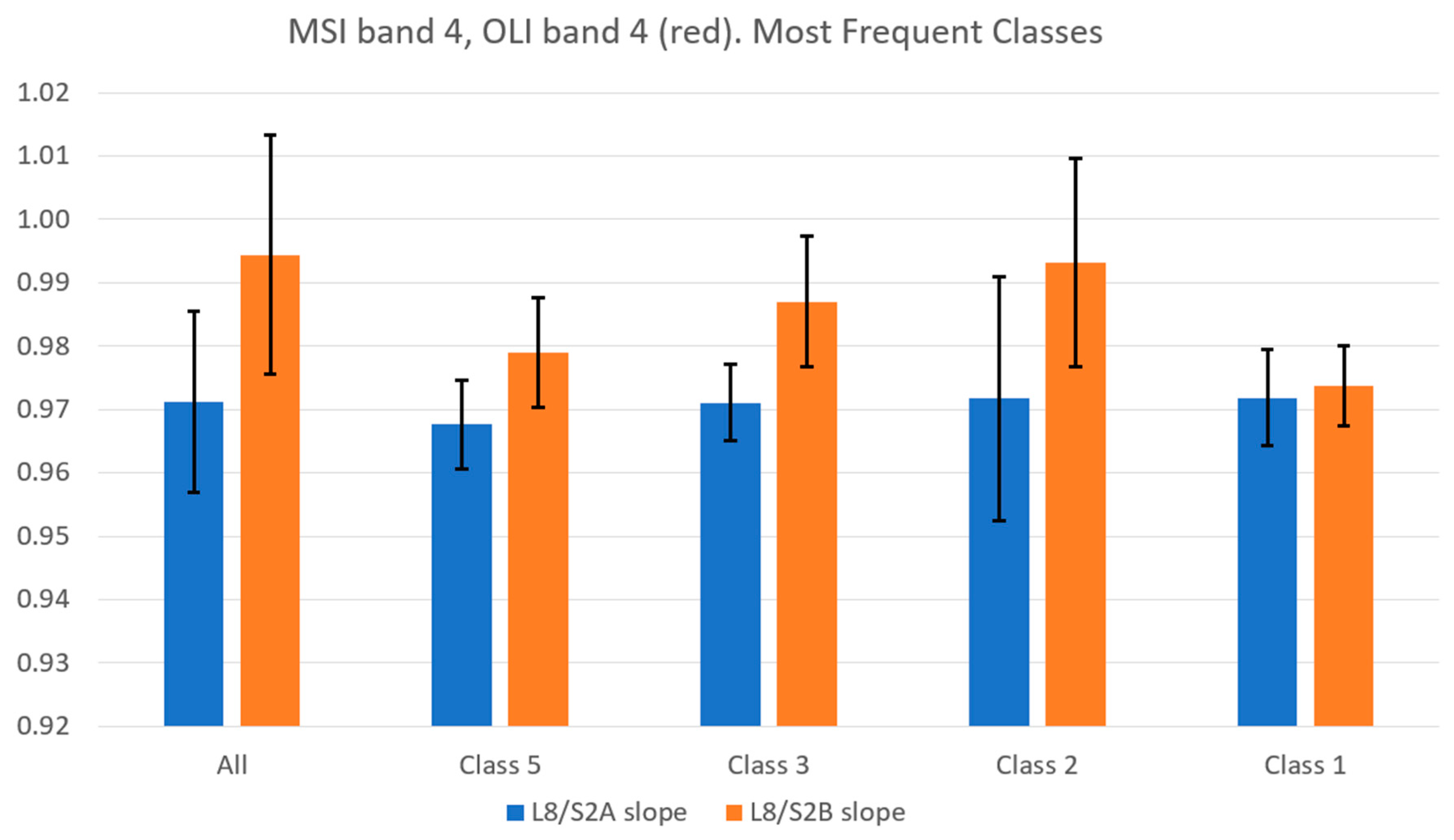
| MSI Band 4, OLI Band 4 (Red). Most Frequent Classes | |||||
|---|---|---|---|---|---|
| Satellite | Slope | Correlation Index | Number of HAs | Class | Class Description |
| S2A | 0.97124 | 0.99741 | 2376 | all | All classes |
| S2B | 0.99444 | 0.99873 | 1702 | ||
| S2A | 0.96765 | 0.99310 | 1558 | 5 | Bare/sparse vegetation |
| S2B | 0.97898 | 0.99876 | 655 | ||
| S2A | 0.97106 | 0.99599 | 142 | 3 | Cultivated and managed vegetation/agriculture |
| S2B | 0.98698 | 0.99378 | 221 | ||
| S2A | 0.97171 | 0.99511 | 471 | 2 | Herbaceous vegetation |
| S2B | 0.99318 | 0.99932 | 152 | ||
| S2A | 0.97181 | 0.99857 | 33 | 1 | Shrubs |
| S2B | 0.97378 | 0.99667 | 158 | ||
© 2020 by the authors. Licensee MDPI, Basel, Switzerland. This article is an open access article distributed under the terms and conditions of the Creative Commons Attribution (CC BY) license (http://creativecommons.org/licenses/by/4.0/).
Share and Cite
Gil, J.; Rodrigo, J.F.; Salvador, P.; Gómez, D.; Sanz, J.; Casanova, J.L. An Empirical Radiometric Intercomparison Methodology Based on Global Simultaneous Nadir Overpasses Applied to Landsat 8 and Sentinel-2. Remote Sens. 2020, 12, 2736. https://0-doi-org.brum.beds.ac.uk/10.3390/rs12172736
Gil J, Rodrigo JF, Salvador P, Gómez D, Sanz J, Casanova JL. An Empirical Radiometric Intercomparison Methodology Based on Global Simultaneous Nadir Overpasses Applied to Landsat 8 and Sentinel-2. Remote Sensing. 2020; 12(17):2736. https://0-doi-org.brum.beds.ac.uk/10.3390/rs12172736
Chicago/Turabian StyleGil, Jorge, Juan Fernando Rodrigo, Pablo Salvador, Diego Gómez, Julia Sanz, and Jose Luis Casanova. 2020. "An Empirical Radiometric Intercomparison Methodology Based on Global Simultaneous Nadir Overpasses Applied to Landsat 8 and Sentinel-2" Remote Sensing 12, no. 17: 2736. https://0-doi-org.brum.beds.ac.uk/10.3390/rs12172736