Calibrating Geosynchronous and Polar Orbiting Satellites: Sharing Best Practices


1
United States Geological Survey Earth Resources Observation and Science Center, Sioux Falls, SD 57198, USA
2
National Aeronautics and Space Administration Langley Research Center, Hampton, VA 23666, USA
3
Science Systems and Applications Inc., National Aeronautics and Space Administration Langley Research Center, Hampton, VA 23666, USA
4
Global Science & Technology, National Oceanic and Atmospheric Administration, Greenbelt, MD 20770, USA
5
Science Systems and Applications Inc., National Aeronautics and Space Administration Goddard Space Flight Center, Greenbelt, MD 20771, USA
*
Author to whom correspondence should be addressed.
Remote Sens. 2020, 12(17), 2786; https://0-doi-org.brum.beds.ac.uk/10.3390/rs12172786
Submission received: 23 July 2020
/
Revised: 17 August 2020
/
Accepted: 25 August 2020
/
Published: 27 August 2020
(This article belongs to the Special Issue Cross-Calibration and Interoperability of Remote Sensing Instruments)
Abstract
:Earth remote sensing optical satellite systems are often divided into two categories—geosynchronous and sun-synchronous. Geosynchronous systems essentially rotate with the Earth and continuously observe the same region of the Earth. Sun-synchronous systems are generally in a polar orbit and view differing regions of the Earth at the same local time. Although similar in instrument design, there are enough differences in these two types of missions that often the calibration of the instruments can be substantially different. Thus, respective calibration teams develop independent methods and do not interact regularly or often. Yet, there are numerous areas of overlap and much to learn from one another. To address this issue, a panel of experts from both types of systems was convened to discover common areas of concern, areas where improvements can be made, and recommendations for the future. As a result of the panelist’s efforts, a set of eight recommendations were developed. Those that are related to improvements of current technologies include maintaining sun-synchronous orbits (not allowing orbital decay), standardization of spectral bandpasses, and expanded use of well-developed calibration techniques such as deep convective clouds, pseudo invariant calibration sites, and lunar methodologies. New techniques for expanded calibration capability include using geosynchronous instruments as transfer radiometers, continued development of ground-based prelaunch calibration technologies, expansion of RadCalNet, and development of space-based calibration radiometer systems.
1. Introduction
Two main categories of optical Earth observation satellites are geosynchronous (those that continuously stare at the same area of the Earth’s surface) and sun-synchronous (or polar-orbiting—those that can observe differing areas of the Earth’s surface at the same time each day). Both types of systems have critical needs for radiometric and geometric calibration of their sensors in order to conduct their missions. However, the procedures developed for calibration by the respective instrument teams are highly refined but substantially different due to the differing orbits. As a result, calibration teams for these two types of sensors do not often interact. Even so, since the fundamental goal of accurate image calibration remains the same, there are large areas of overlap between the two calibration communities that likely have not been extensively explored, compared, contrasted, and employed for improving calibration methodologies. In response to this observation, a workshop was developed to bring representatives from these two calibration communities together in order to explore opportunities for expanded interaction with each other to improve best practices of radiometric calibration for these types of orbital sensors as well as for the greater optical remote sensing community.
The workshop concept was to bring together a panel of experts to discuss capabilities and limitations that define the current practice in the calibration of sun-synchronous and geosynchronous optical remote sensing satellites and to determine a path forward for calibration improvement based on synergies identified between the two groups. Panel members presented their perspectives on the topic and then interacted extensively with the goal of producing recommendations useful for both calibration communities, as well as for broader implementation.
On 23 September 2019, the workshop was held at the U.S. Geological Survey (USGS) headquarters in Reston, Virginia, United States, to address the issue. It was a one-day workshop designed to allow a select group of panelists to interact extensively on the question of “Calibrating Geosynchronous and Sun-synchronous Satellites: Sharing Best Practices.” Each of the eight panelists presented their position on the topic in the morning session, and the afternoon was devoted to discussion amongst the panelists as well as with the audience. In particular, the panelists were asked to frame their thoughts around the following four key questions:
- What are the radiometric/geometric/spatial calibration capabilities of sun-synchronous polar orbiting instruments such as Landsat Operational Land Imager (OLI), Moderate Resolution Imaging Spectroradiometer (MODIS), and Sentinel 2 Multispectral Instrument (MSI)?
- What are the radiometric/geometric/spatial calibration methodologies of geostationary instruments such as those carried on the United Sates Geostationary Operational Environmental Satellite (GOES), European Organization for the Exploitation of Meteorological Satellites (EUMETSAT), and Japanese Himawari Satellites?
- With respect to calibration capabilities, what are the limitations of each type of system and the differences between system types?
- What activities can be implemented to optimize the calibration of both sets of systems?
Panelists were chosen based on their experience in calibrating sensors of this type. Some were primarily involved with geosynchronous sensors, others with sun-synchronous sensors, and some had experience in both areas. Table 1 provides a list of panel members along with their affiliations.
2. Background
Low Earth Orbit (LEO) is characterized by an altitude of 160 to 2000 km; Earth observing instruments can be placed in LEO orbit at lower cost than higher orbits. LEO orbits are ideal for Earth remote sensing because near-polar orbits (inclinations of around 98°) can be sun-synchronous—that is, the satellite crosses the equator at the same local time during each orbit. This guarantees that the solar illumination is essentially zonally constant except for seasonal effects. The imaging sensor can be designed to generate a daily global mosaic consisting of contiguous orbits with the same local equator time. The sensors also observe regions near both poles during every orbit. These designs are especially useful for monitoring long-term changes of land use or cloud properties due to the local time consistency (i.e., no diurnal impact) of the observations. The low-altitude orbit also facilitates high spatial-resolution imaging.
In contrast, satellites in Geosynchronous Equatorial Orbit (GEO) have an orbital period of one sidereal day. These orbits are characterized by a much higher altitude—approximately 35,786 km. Thus, it is much more expensive to place satellites into this orbit due to the need for larger rockets. In a geostationary orbit, which is a special geosynchronous orbit with zero eccentricity and inclination angle, the satellite essentially maintains its location above a fixed point on the Earth’s surface. This type of orbit is ideal for constant observation of the same portion of the Earth each day, which is especially useful for meteorological observations (e.g., severe weather and hurricane tracking as well as observing the regional diurnal cycle of clouds) and for many communications systems. About five GEO satellites are needed to have contiguous coverage over the tropics. However, solar illumination angles change dramatically throughout the sunlit portion of the day, which can have a serious impact on remote sensing applications.
3. Opportunities for Improving Current Calibration Capabilities
3.1. Criticality of Maintaining Current Sun-Synchronous Orbit
The sun-synchronous orbit grants opportunities for daily observation of the entire Earth for the same zonal illumination conditions, which is important for monitoring the Earth’s weather systems. Additionally, the instruments’ low altitude allows for high spatial-resolution imagery. Unfortunately, the low altitude also makes the satellites susceptible to orbital decay. If no corrective actions are taken, the altitude and inclination will not be coordinated in order to maintain a sun-synchronous orbit. The National Oceanic Atmospheric Administration (NOAA) 1–19 satellite constellation was not maintained, and gradually, the local equator crossing times (LECT) drifted toward the terminator within a few years. Most all contemporary polar orbiting satellites are sun-synchronous, such as Landsat, Metop, FengYun-3 (FY-3), and Joint Polar Satellite System (JPSS). The panel recommends that future LEO missions designed for climate studies have maintained orbits.
Recently, there has been a push toward single-sensor small satellites and CubeSats in order to reduce costs and scheduling impacts. Maintaining a CubeSat orbit is challenging with current technology, but new propulsion systems are being developed [1]. For example, aerodynamic inclination correction could be used to maintain the LECT, which uses much less fuel than conventional orbit maneuvers [2]. Additionally, adjusting the injection inclination may provide a few more years of a stable LECT [3]. Such techniques would allow a series of CubeSat sensors to be injected in close-proximity orbits to synergistically study cloud, aerosol, land use, and other environmental retrievals, similar to the A-train [4].
Cloud, land use, aerosol, and other environmental retrievals based on maintained sun-synchronous orbits allow for long-term climate modelling because the regional diurnal variations are not aliased into the long-term trend. There have been many attempts to unravel the regional diurnal changes in retrieval properties from long-term monitoring, with much more work to be done [5,6,7,8,9]. Another consideration is that if there are solar zenith angle (SZA) dependencies in the retrieval algorithm, they would manifest themselves along with the true long-term change in degrading orbit records. In order to quantify the regional diurnal cycle of retrievals, precessionary and GEO orbits are best suited for these studies [10,11,12].
The GEO orbit allows the Earth to be scanned on a pre-determined schedule. The satellites are developed with coordinated scanning patterns and have, to a reasonable extent, maintained longitudinal consistency since the 1980s in support of the International Satellite Cloud Climatology Project (ISCCP) [13]. The GEO scanning schedule allows a desert or other pseudo invariant calibration sites (PICS) [14] to be observed at the same local time. The consistent local-time sampling ensures that daily SZA conditions are repeated every year, allowing for construction of an empirical bidirectional reflectance distribution function (BRDF) using one GEO that can then be applied to another GEO in similar positions [15]. For example, over Saharan Africa, the largest SZAs are experienced in winter, and near-nadir conditions in summer. The seasonal surface and atmospheric conditions over the PICS can then be correlated with the SZA.
Similarly, the daily-observed PICS SZA repeats annually for a sun-synchronous satellite maintained at a given LECT. In this case, an empirical BRDF can be constructed using measurements from the first few years after launch—the time during which sensor degradation effects are most unlikely [16]. The empirical BRDF can then be used to monitor the stability of the sensor during its lifetime. The advantage of the empirical BRDF is that it has been optimized for the sensor spectral response function and the seasonal atmospheric and surface conditions specific for each PICS [17]. These considerations, therefore, reduce reliance on radiative transfer models based on monitored ground site measurements or theoretically derived BRDFs. If the follow-on sensors are in the same LECT orbit, the empirical BRDF from the previous sensor can be used to track the stability of the later one soon after launch [18]. Sensors in degrading orbits have been inter-calibrated, but the uncertainty of the inter-calibration increases significantly as the orbits drift toward the terminator [19,20,21,22].
Given the current availability of Aqua, National Polar-orbiting Partnership (NPP), and JPSS, a continuous record of climate-quality, inter-calibrated, and overlapping 1:30 PM LECT sensors is anticipated for the next several years. The seamlessly combined sensor record can then be scaled to an absolute on-orbit traceable calibration reference, such as Climate Absolute Radiance and Refractivity Observatory (CLARREO) PATHFINDER mission on the International Space Station (ISS) in the 2020s [23,24]. The uncertainty of transferring the CLARREO calibration reference throughout the entire overlapping sensor record is reduced by inter-calibrating based on the 1:30 PM LECT orbit.
3.2. Spectral Standardization
The MODIS and Visible Infrared Imaging Radiometer Suite (VIIRS) cloud retrieval teams have released a combined consistent MODIS and VIIRS cloud property dataset [25]. They considered the number of bands and band spectral response function (SRF) differences, pixel size including aggregation and the bowtie effect, and channel calibration differences. To achieve multi-satellite climate-quality retrieval datasets, exact sensor copies (ideally orbiting in the same LECT) are best-suited for ensuring consistent channels, SRFs, and pixel size.
The sensor SRF observed reflectance differences are scene type dependent and, therefore, so are corrections factors derived from them. The scene type determines the Earth spectral reflected radiance condition, which is influenced by surface/cloud variance and the atmospheric column. The radiometric scaling factor between the reference and target sensor simply accounts for the calibration difference between the two on-orbitcalibration systems and/or vicarious methods. If both sensor SRFs were identical, then all the simultaneous nadir overpass (SNO) or ray-matched Earth scene reflectance differences would reveal the same radiometric scaling factor. If the sensor bands are similar but the SRFs differ, then the scene-type-induced reflectance differences must be properly removed [26]. This radiometric scaling factor does not provide specific scene-type-corrected reflectances. Such a correction is best handled by the retrieval algorithm, which identifies the proper scene type to determine the associated reflectance difference required to obtain similar measurements.
By convolving the target sensor band SRF with coincident collocated and ray-matched hyperspectral reference sensor radiances, the scaling factor can easily account for the SRF differences. All the target sensors would then be radiometrically scaled to the same hyperspectral reference sensor. The Global Space-based Inter-Calibration System (GSICS) is an international collaborative effort among sensor agencies to employ calibration best practices in order to achieve harmonized measurements [27]. GSICS currently uses Infrared Atmospheric Sounding Interferometer (IASI) hyperspectral infrared (IR) radiances to radiometrically scale IR target sensors [28]. The CLARREO approach will radiometrically scale visible-near-infrared (VIS-NIR) visible sensors to the CLARREO PATHFINDER hyperspectral International System of Units (SI) traceable radiances [23,24].
Currently, there are no VIS/NIR hyperspectral sensors that cover the full extent of the solar-reflected wavelengths with sufficient resolution or operation schedule. Therefore, scene-specific Spectral Band Adjustment Factors (SBAF) are required to inter-calibrate two sensor bands [29]. Historically, sensors were calibrated using risk terrain modelling RTM-predicted at-sensor radiances based on clear-sky desert target in-situ surface reflectance and atmospheric measurements [30]. Alternatively, one can utilize the SCIAMACHY hyperspectral (240–1700 nm) trace gas sensor, which operated between 2002 and 2012 [31]. By convolving the target and reference SRF with SCIAMACHY hyperspectral reflectance over a given scene type, with similar solar and viewing conditions as required by a target and reference sensor inter-calibration event, a suitable SBAF can be determined [32,33]. The web-based SBAF tool allows the user to reduce the associated SBAF uncertainty by customizing the tool to account for the unique conditions associated with different inter-calibration techniques (https://cloudsway2.larc.nasa.gov/cgi-bin/site/showdoc?mnemonic=SBAF). Furthermore, selecting scene types that are spectrally flat within the two spectral bands can reduce the impact of the SRF differences. For example, deep convective clouds (DCC) are effectively spectrally flat for wavelengths less than 1 µm [34]. Note that DCC are not well-suited for inter-calibration across the 1.6 µm band because the reflectance is dependent on particle size, and DCC are not highly reflective at this wavelength [35]. The 1.6 µm desert target reflectance is very bright, however. For the 1.38 µm band, only high clouds are visible, thus limiting inter-calibration efforts to DCC targets [36].
3.3. Expanded DCC-Based Calibration
Tropical deep convective clouds (DCC) are an excellent invariant Earth target for radiometric calibration of satellite sensors. Compared to ground PICS, they are significantly less impacted by water vapor absorption, offer high signal-to-noise ratio (SNR), and are nearly Lambertian in the visible and near-infrared solar spectrum [18,34]. Found globally across tropical domains, DCC are applicable for calibrating imagers on both GEO and LEO orbits. Unlike the PICS approach, for which the spatially averaged top-of-atmosphere (TOA) reflectance over an invariant ground site is regarded radiometrically and temporally stable over time, the DCC calibration technique is a large-ensemble statistical approach that relies on the assumption that the distribution of DCC reflectance in the visible spectrum remains constant in time. The baseline DCC method, as described by Doelling et al. [34], uses an 11 µm IR channel brightness temperature threshold of 205 K to identify the DCC pixels over the tropics. The DCC pixel level radiance or reflectance values are compiled into monthly probability distribution functions (PDF), and their statistical mode is tracked over time as a means for monitoring the sensor stability. Prior to the construction of the PDF, the DCC pixel anisotropy is corrected using the angular distribution model (ADM) derived by Hu et al. [37]. Previous studies [16,18] have reported that DCC exhibits a very stable (<1%) and more robust time series of satellite sensor response in the VIS-NIR bands (<1 µm) than any other Earth invariant target. However, at shortwave infrared (SWIR) bands (>1 µm), the DCC reflectivity is affected by ice particle size [35] and is more sensitive to viewing and solar illumination geometry and brightness temperature threshold. The baseline DCC technique, therefore, exhibits large seasonal cycles (up to 3%) in the SWIR band DCC response that significantly affects the detection of trends in these bands [17,18,38].
Recently, Bhatt et al. [17,39] revised the baseline DCC approach to extend its effective application to SWIR bands. A key step in the revised method is the band-specific characterization of the DCC reflectivity as a function of solar zenith angle (SZA), viewing zenith angle (VZA), and relative azimuth angle (RAA) using empirically derived look-up table (LUT) BRDF models that are formulated using the first five years of Suomi National Polar-Orbiting (SNPP)-VIIRS DCC measurements acquired globally near the tropics. The VIIRS-based LUT BRDFs for the VIS-NIR bands look similar and resemble the Hu angular distribution model closely. However, the DCC BRDF patterns were found unique for each of the SWIR bands. Figure 1a shows the comparison between the Hu ADM and the LUT BRDF for the 1.38 µm channel (M9) on SNPP-VIIRS for SZA = 22.5°. The BRDF factor (χ) is nearly symmetric about RAA = 90° for the Hu model, which is valid for VIS-NIR wavelengths. On the other hand, the M9 band reflectance is non-symmetric about the RAA and exhibits a greater reflectance in the forward-scattering direction (RAA < 90°). These contrasting BRDF features imply that a wavelength specific BRDF is necessary for employing the DCC method for SWIR bands. The application of these LUT BRDF models was shown to effectively reduce the SWIR band DCC temporal variability by up to 65% [40]. Figure 1b shows the normalized DCC reflectance time series for SNPP-VIIRS M7 (0.86 µm) and M9 bands with (red triangles) and without (black triangles) the BRDF corrections. The application of Hu ADM reduces the temporal standard error by more than 50% in the M7 band DCC time series. The M9 band is located in a strong atmospheric absorption band, and the ground PICS are not visible with this spectral channel. Therefore, the high-altitude DCC are the only invariant Earth targets available for vicarious calibration of the 1.38 μm band. The application of the LUT BRDF reduces the temporal natural variability of the VIIRS M9 band DCC response to less than 1%. Bhatt et al. [40] showed that the revised DCC approach can detect an instrument degradation trend of <1%/decade in all reflective solar bands at the 5% significance level (or 95% confidence level) and 50% probability of significant trend detection.
In addition to trend detection, DCC can also be used for absolute radiometric inter-comparison between two LEO imagers in the same orbit [40]. SNPP-VIIRS and Aqua-MODIS are both in a 13:30 sun-synchronous orbit, and as such they have consistent local time sampling of the DCC cycle. This avoids any diurnal sampling differences of DCC properties between the two instruments. By normalizing the DCC acquisitions from the two instruments to similar angular and viewing conditions using the Hu ADM for VIS-NIR and channel-specific LUT BRDF for SWIR bands, the radiometric inter-comparison between the matching spectral bands of Aqua-MODIS and SNPP-VIIRS was performed. The results show an excellent agreement (within 1%) with those obtained from direct ray-matching between these two instruments over all-sky tropical ocean scenes. The DCC method, therefore, can be used as a reliable independent approach for cross-calibration between two sensors, and is particularly useful when ray-matched or simultaneous observations are not possible. Most of the DCC work reported so far is with moderate resolution (~1 km) imagers. The panel recommends exploring the applicability of the revised DCC method with high-resolution satellite imagers, such as Landsat sensor series.
3.4. Extended Pseudo Invariant Calibration Sites Techniques
Pseudo Invariant Calibration Sites, or PICS, have been used extensively for on-orbit calibration of optical remote sensing instruments for the past two decades. The initial work in this area was performed by Cosnefroy et al. [41] in 1996 where several sites were characterized in the North African Sahara Desert. This work has been extended significantly by many calibration groups worldwide and is now a recommended calibration approach endorsed by the Committee on Earth Observation Satellites Working Group on Calibration and Validation Infrared Visible and Optical Subgroup (CEOS WGCV IVOS) (http://calvalportal.ceos.org/pics_sites;jsessionid=E23DEDA838DBA64C000749A00E0815A0). The basic assumption behind PICS calibration is that these locations on the Earth’s surface do not change with time. Thus, if they are monitored by a satellite sensor, and corrections for viewing and illumination geometry are made, any observed changes are due to the sensor rather than the PICS. Figure 2 shows a recent example of trending analysis for Landsat 8 OLI using a well-known PICS named Libya 4. This figure illustrates the high reflectance obtainable from Saharan PICS as well as the stability exhibited by OLI. If only temporal stability is considered, uncertainties are below 1% in each spectral channel except for SWIR-2 where the temporal uncertainty is 1.8%. After development and application of an effective TOA BRDF model, this type of stability can be achieved for many PICS across the Sahara. Residual uncertainties are primarily due to atmospheric changes that occur on a daily as well as an annual scale. Because of the nature of the Sahara Desert, cloud cover is less of an issue and many sites can be observed on the order of 60–70% of the time, with slightly better performance during the summer months.
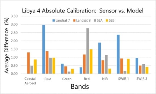
Absolute radiometric calibration using PICS has also been developed [42,43,44]. Use of PICS for absolute calibration of optical remote sensing instruments requires incorporating either a calibrated source, normally the sun, or a calibrated sensor (radiometer), normally a well-accepted sensor system (an example would be MODIS Terra) already on orbit. Thus, fundamentally, the accuracy of the model is primarily dependent on the accuracy of the corresponding source or sensor. An example of absolute radiometric calibration using a model developed for Libya 4 by South Dakota State University is shown in Figure 3. Average results of using the model to predict TOA reflectance for Landsat 7, 8 and Sentinel-2 A, B sensors are shown. For this model the average difference between model predictions and sensor measurements is less than 3% in all cases and approaching 1% or better for several sensor/band combinations. This model is based on the MODIS Terra sensor and, at the very least, shows excellent agreement among all five sensors. These results suggest potential for PICS to yield absolute calibration models with accuracies of 3% or better.
Fundamentally, PICS are useful for both sun-synchronous and geosynchronous sensors. However, while sun-synchronous sensors will normally view any given PICS on a regular basis, geosynchronous sensors essentially stare at the same portion of the Earth’s surface continually. Thus, there is the distinct disadvantage that some PICS will never be observed, and the distinct advantage that other PICS may be observed on an almost continuous basis. It is imperative, therefore, that PICS are located as globally as possible. Fortunately, algorithms and recommendations were developed to accomplish this [45]. As an example, GOES-East and GOES-West are designed to monitor the continental United States as shown in Figure 4. Neither can monitor Saharan PICS, however, both can continuously monitor the Sonoran Desert PICS (indicated by red star in Figure 4). Unfortunately, due to increased influence from vegetation and nearby water bodies, the Sonora Desert is not as stable as Saharan sites (Figure 5). However, for applications of cross-calibration of sensors, there is a tremendous advantage to exploiting the observations of geosynchronous sensors such as GOES-East and GOES-West coupled with observations of sun-synchronous sensors such as MODIS, Landsat, and Sentinel-2. While geosynchronous sensors are limited in viewing angle, they can track illumination angle through the day. Conversely, sun-synchronous sensors are limited in illumination angle, but can provide additional viewing angles (compared to geosynchronous view angles, which can be limited to extremely off-nadir looks). Thus, by integrating all these observations together, and taking advantage of the substantial increase in observations, many of these uncertainties can potentially be reduced leading to substantial improvement in the use of the Sonora Desert as a PICS. Other examples are possible worldwide. This is a largely unexploited area of calibration activity that should be more aggressively pursued.
Another distinct advantage of PICS is that if they are indeed invariant over time, then they can be used for historical calibration purposes. Weather satellites have been monitoring the Earth’s surface since the early 1960s. Land remote sensing began with the Landsat series when Landsat 1 was launched in 1972. Landsat has recorded the Earth’s surface continually since then, using more than nine sensors. The Sonora PICS was used to perform a cross-calibration of the entire Landsat suite as shown in Figure 6. This figure shows that continuity through the history of Landsat can be developed through use of PICS. This concept can be extended to both current and historical sun-synchronous and geosynchronous sensors.
Developments in PICS-based calibration have continued to grow and one that is pertinent to this topic is the concept of extending PICS from point sites to areal sites. To date, PICS are generally of small extent—a few kilometers—and can only be observed intermittently by most sun-synchronous systems. However, recent analysis has shown that the Sahara Desert consists of only a handful of surface cover types and, correspondingly, only a handful of surface reflectance models [46,47]. All of North Africa can possibly be a calibration site and observations by sun-synchronous sensors of extended PICS (EPICS) can be done far more often. Observations of PICS with sun-synchronous systems will lead to better modeling of PICS, improved uncertainties based on PICS-based calibration, and better characterization of sensors that may have limited radiometric stability.
In summary, PICS-based calibration has proven itself highly useful for both geosynchronous and sun-synchronous sensors. Recommendations include continued development of improved PICS models and, especially, improvements in PICS-based calibration through coordinated efforts involving both sun-synchronous and geosynchronous sensor calibration groups.
3.5. Improved Lunar Calibration
Reliable radiometric calibration depends on high-precision radiometric prelaunch and on-orbit calibration of the imaging sensor. Besides Earth-based vicarious calibration approaches such as DCC and SNO, the moon has become a standard alternative source of irradiance that serves as a Solar Diffuser (SD)-like reference for on-orbit radiometric calibration. There are two clear advantages of using the moon’s surface for radiometric calibration. First, the lunar surface does not degrade over time; thus, we do not have to monitor the degradation of the moon as is done with the SD or Solar Diffuser Stability Monitor (SDSM) for the VIIRS or MODIS sensors. Second, lunar calibration is not impaired by atmospheric transmission as is Earth-view-based calibration. Despite these two advantages, lunar calibration requires an accurate prediction or estimation of the lunar irradiance model to track sensor change over time. The spectral responses and reflectance characteristics of the moon were studied by Kieffer and Stone et al. for an extended period [48,49]. The Robotic Lunar Observatory (ROLO) model was developed by the U.S. Geological Survey (USGS) providing lunar irradiance for remote sensing sensors in the wavelengths between 0.35 and 2.39 um [48]. In addition, Miller and Turner [50] also developed a lunar spectral irradiance database (MT2009) for VIIRS Day Night Band (DNB) calibration covering a spectral range from 0.3 um to 2.8um. Later, a study demonstrated that the relative (not absolute) accuracy of the ROLO lunar irradiance model was better than the MT2009 model [51]. In addition to LEO satellites, GEO sensors also used the moon as a part of on-orbit calibrations. Wu et al. [52] used scheduled and unscheduled moon collections from NOAA’s Geostationary Operational Environmental Satellite 10 (GOES-10) in the visible channels since it did not include an onboard calibration source. In addition, Bremer emphasized the importance of lunar calibration for GOES-R Advance Land Imager (ABI) since ABI scans the moon in the Field Of Regard (FOR) without any space maneuver.
In this section, a common approach for lunar calibration is described, and its corresponding results are also provided in terms of SNPP and NOAA-20 VIIRS. In the later part of this section, methodology and results of the cross-calibration between the two VIIRS sensors are briefly presented along with recommendations for lunar calibration improvements.
3.5.1. Methodologies
The first step of lunar calibration is predicting opportunities for viewing the moon through the Space View (SV) port with the spacecraft roll maneuver. The monthly scheduling steps are well described in Wilson’s study [53]. After the planned lunar roll maneuver, VIIRS is able to acquire the moon through the SV port near the desired phase angle of −51 degrees. The negative sign of the phase angle indicates that the moon is in the waxing phase.
At the time of scheduled lunar collection, the lunar irradiance is derived by the GSICS developed Implementation of the ROLO (GIRO) model. GIRO was developed under the lead of the European Organization for the Exploitation of Meteorological Satellites (EUMETSAT) based on the ROLO model in coordination with international space agencies. After bias correction using the dark space digital numbers (dn), the radiance values of the lunar pixels were derived by using the c-coefficients in Equation (1).
In Equation (1), b is band, d is detector, h is half angle mirror side, f is frame, s is sub-frame, and t0 is the initial on-orbit calibration gain (known as F-factors for VIIRS). Since GIRO provides an expected lunar irradiance value at the time of the lunar collection, the lunar radiance calculated in Equation (1) needs to be converted to irradiance by applying the moon solid angle and effective area ratio of the moon from the solid angle as shown in Equation (2).
In Equation (2), IGIRO(b) is the irradiance from the GIRO model, IOBS(b) is the observed lunar irradiance, Rmoon is the radius of the moon, Dsat_moon is the distance between the moon and satellite, is the phase angle of the moon, N is the number of effective pixels.
3.5.2. Cross-calibration of the SNPP and NOAA-20 VIIRS Methodology
The scheduled lunar collections for the NOAA-20 and S-NPP VIIRS sensors were performed the same day with small time differences. For cross calibration of these two sensors, the ratio of observed lunar irradiance calculated from the denominator part of Equation (4) between NOAA-20 and S-NPP VIIRS are calculated using Equation (3).
Since there were collection time differences between them, the reference GIRO irradiance ratio differences should be calculated as shown in Equation (4).
Since the S-NPP VIIRS gain has been stabilized over 8 years of operation, using S-NPP VIIRS as reference, the cross-calibration ratio Rxcal can be calculated by Equation (5).
The calculated ratio Rxcal represents relative detector response changes of NOAA-20 VIIRS over time with the reference S-NPP VIIRS.
3.5.3. Results
(1) S-NPP and NOAA-20 VIIRS SD versus Lunar F-factors
Since there is a large bias in the ROLO model in the absolute radiometric scale because of atmospheric correction error and high uncertainty in Vega absolute irradiance, which is used to scale ROLO, the lunar F-factors can only be used for long-term relative calibration [51]. An optimal scaling factor is calculated by minimizing the differences between the SD F-factors at the time of lunar F-factor calculation in each band as shown in Figure 7. In Figure 7 top plot, the solid line represents SD F-factors and the symbols are the lunar F-factors. The dashed vertical lines are the year division lines and the lunar F-factors are not available from July to October because the moon goes below the Earth limb. The long-term trends between SD and scaled lunar F-factors showed reasonable agreement. The standard deviations of the lunar F-factors to the SD F-factor were less than 1% in all the RSB bands [52].
Like the S-NPP case, the lunar F-factors for NOAA-20 VIIRS were normalized to the SD F-factors at the 2nd lunar collection time as shown in Figure 7, bottom plot. In the VIS-NIR bands, the SD and lunar F-factors showed good agreement—within 1%. In the short wavelength bands (M1~M4), the SD F-factors are linearly deviating from the lunar F-factors in addition to the annual oscillations. In the SWIR bands, SD and lunar F-factors are mostly within the 1% level.
(2) Cross-calibration of the S-NPP and NOAA-20 VIIRS Results
For lunar-based cross-calibration, there were 14 lunar collection pairs available. The lunar cross-calibration ratios are calculated and plotted in Figure 8. Figure 8 shows only bands M1 to M4 in the short wavelength side that had SD and lunar F-factor discrepancies with NOAA-20 VIIRS.
Based on SNPP lunar F-factors, cross-calibration is performed on NOAA-20 VIIRS lunar F-factors. Cross-calibration ratio results were tighter than original lunar F-factor trends in Figure 8. Band M1 decreased approximately 1% over the 1.5 years of NOAA-20 operations. This observation is similar to the SD and lunar F-factor comparison chart in Figure 3. Again, these results are true when the SNPP-VIIRS lunar F-factors are stabilized and represent the true sensor responsivity status in this study period. Besides band M1, bands M2—M4 show almost no sensor changes over time.
3.5.4. Summary of Lunar Calibration Techniques
As an alternative source of on-orbit radiometric calibration, the moon has been frequently used for GEO and LEO remote sensing instruments such as VIIRS and GOES ABI. This section focused on the two VIIRS sensors on the SNPP and NOAA-20 satellites in comparison with SD-based primary calibrations. However, there are small time-dependent long-term deviations in the short wavelength bands (M1–M4); SNPP showed very good agreement between the lunar and SD F-factors. Over eight years of operation, they were mostly within the 1% standard deviation of the lunar F-factor residues when they were compared to the SD F-factors at the time of lunar collection. Similarly, NOAA-20 VIIRS showed approximately 1% deviations between the SD and lunar F-factors, however, these differences need to be validated by other vicarious results such as long-term DCC or PICS. On the other hand, a lunar cross-calibration methodology has been applied to track lunar calibration-based detector responsivity changes. For the short wavelength bands (M1–M4), the initial results indicated that there could be approximately 1% radiometric responsivity changes within the 1.5 year comparison period. For the other bands, the long-term trends need to be built-up to make further decisions. In these applications, lunar-based calibration in the visible region has shown accuracy potential to 1%. Current limitations to the ROLO model seem to be based on uncertainties due to atmospheric interference and knowledge of the absolute radiance of Vega. Panel recommendations include addressing these limitations in order to achieve the sub-1% potential that lunar calibration can produce throughout the VNIR and SWIR spectrum.
3.6. Using GEO as a Transfer Radiometer
The current operational plan to integrate NPP and JPSS satellites into the same orbit is an effort to equally space them to better monitor severe weather events (https://www.jpss.noaa.gov/mission_and_instruments.html). This is also the operational procedure of the Metop A/B/C satellite series located in a 9:30 AM LECT synchronous descending orbit (https://directory.eoportal.org/web/eoportal/satellite-missions/m/metop#Po3DN1eHerb). Direct inter-comparisons are not possible between satellite sensors in these staggered orbital configurations. Well-characterized PICS, however, can be used to determine the calibration difference between these sensors, although the complete dynamic range cannot be sampled using individual PICS due to their limited reflectance variance. Similarly, not all scan positions can be monitored using region-of-interest-based PICS, such as desert and polar ice targets, due to the limited repeat cycle of these orbits (16 days for NPP https://directory.eoportal.org/web/eoportal/satellite-missions/s/suomi-npp). However, all scan positions can be monitored using DCC because they are analyzed collectively over the tropics [54]. Analogously, by combining multiple North African locations of similar spectral response as if they were one site allows all orbit crossings to be utilized for stability monitoring of a sensor, and to quantify scan position dependencies [47].
The advent of the third-generation GOES sensors, which currently include Himawari-8/9, GOES-16/17, and GEO-KOMPSAT-2A/B, has provided optimal transfer radiometers between JPSS sensors. The full disk imaging can be scheduled every 10 minutes, allowing all coincident ray-matched observations to be within 5 minutes. At least three daily sun-synchronous orbit crossings can be ray-matched over the GEO domain. The frequent orbital crossings allow for the daily monitoring of either GEO or LEO sensor L1B radiance anomalies [55]. The GOES band SRFs are similar to those of VIIRS, which allows the potential for consistent environmental retrievals, such as aerosol optical depths, across MODIS, VIIRS, and Himawari-8 sensors [56]. The GOES and VIIRS visible pixel fields of view (FOVs) are 1 and 0.75 km, respectively, which are reasonably comparable for near-nadir ray-matched observations. This similarity facilitated determination of navigation accuracy of GOES-16 with respect to NPP-VIIRS by using coincident SNO GOES-16 and NPP-VIIRS images [57]. The NASA Clouds and the Earth’s Radiant Energy System (CERES) project has used all-sky tropical ocean (ATO) ray-matching to calibrate 20 GEOs to the same Aqua-MODIS C6 calibration reference [58,59]. The full dynamic range of Earth-reflected radiances can be observed by ray-matching over ATO conditions. The Multi-functional Transport Satellite (MTSAT)-1R visible band non-linear response was found using ATO ray-matches with Aqua-MODIS band 1, which was determined to be caused by a small radiance contribution source from locations several hundred kilometers distant from the MTSAT-1R pixel center [60]. Analogous to ATO ray-matching, the VIIRS linear response can be determined using solar eclipse conditions [61]. The GOES sensors are well-suited for use as transfer radiometers via ATO ray-matching for the purpose of determining the calibration difference between VIIRS sensors in the same orbit [62], as well as between the Aqua-MODIS and NPP-VIIRS sensors, which are located in differing LECT sun-synchronous orbits [16].
4. New Opportunities for Calibration Improvement
4.1. Goddard Laser for the Absolute Measurement of Radiance
The Goddard Laser for the Absolute Measurement of Radiance (GLAMR) is a mobile GSFC-based test facility, developed to facilitate the spectral characterization and absolute calibration of typical Earth remote sensing instruments. GLAMR is based on the National Institute of Standards and Technology (NIST) Spectral Irradiance and Radiance Calibrations using Uniform Sources (SIRCUS) facility [63], though the capabilities of GLAMR have expanded beyond the original traveling version of SIRCUS.
The heart of the GLAMR facility is a collection of tunable laser systems that can collectively lase at any wavelength between 340 and 2500 nm. The outputs of the laser systems are coupled to a 30 in diameter integrating sphere via fiber optic cables. The radiance inside the sphere is monitored by three permanently mounted radiometers, so called sphere monitors (Figure 9). These radiometers stare at the back of the sphere, at the same location an instrument in front of the sphere would see. The NIST-traceable absolute calibration is transferred to the sphere monitors via a set of transfer radiometers that are regularly calibrated by NIST, with accuracies between 0.1 and 1% (k = 1). Maximum signal levels vary based on spectral region but range from several milliwatts to several Watts and are generally tunable to the noise floor of the instrument. Spectral traceability is achieved by continuous measurement of the laser system output by laser spectrum analyzers and wavemeters, with accuracies of 0.01 to 1 Å, depending on the spectral region.
For a test campaign, GLAMR travels to the instrument to be calibrated and/or characterized. The integrating sphere provides uniform, monochromatic, stable illumination at a known radiance to the instrument to be tested. The NIST-traceable absolute calibration of the output of the GLAMR sphere allows the data to be used for more than just characterizing an instrument’s relative spectral response. The absolute spectral response, and thus absolute radiometric calibration, can be derived from the measurements. Linearity and polarization can also be characterized.
Uncertainties in GLAMR’s absolute calibration are currently better than 1% (k = 1) across the 340–2500 nm spectrum. GLAMR will be used to provide an independent calibration for the CLARREO Pathfinder HySICS instrument, with requirements of uncertainties better than 0.3% (k = 1), so additional refinement of the GLAMR calibration uncertainties are ongoing.
Instrumentation such as GLAMR provides an unprecedented capability for improvement of ground-based calibration of optical satellite systems. Use of GLAMR for both geosynchronous and sun-synchronous systems is recommended. Continued improvement of GLAMR and development of similar systems for enhanced portability and instrument cross-calibration is also strongly recommended.
4.2. RadCalNet Extension
One important example of improvement to vicarious calibration has been the development of the RadCalNet program [64]. Historically, vicarious calibration has been done through the deployment of teams into the field during satellite overpass. The team collects surface and atmospheric information as the satellite views the surface at that location, then processes the data to predict TOA radiance and/or reflectance. This approach has been very successful; however, it is quite expensive and, therefore, deployments can only be made at irregular intervals. The RadCalNet project has sought to automate this method of calibration through deployment of field equipment that provides continuous measurements of surface and atmosphere without the requirement of personnel on-site. Using this approach, measurements can be acquired every day of the year, greatly expanding the opportunities for satellite calibration.
Currently, RadCalNet sites span four continents: Railroad Valley, United States, La Crau, France, Baotou, China, and Gobabeb, Namibia. This is an excellent start for the program and initial results using these sites with a variety of sensors have shown limitations and led to continual improvement in the data that are collected. Improvements to the program, from the standpoint of both sun-synchronous and geosynchronous sensors would be to consider those sensors with large footprints. Only Gobabeb and Railroad Valley can accommodate sensors with 1 km FOVs. Expansion of RadCalNet sites to include more opportunity for coarse resolution sensors would be a major step forward for the geosynchronous community. In addition, RadCalNet data are only available for nadir viewing angles, which can prove difficult for geosynchronous sensors. For example, both GOES-East and GOES-West can view Railroad Valley. However, the viewing angles are decidedly non-nadir. Efforts to incorporate bidirectional reflectance models to accommodate non-nadir viewing angles would be a major step forward for both geosynchronous as well as many sun-synchronous sensors that do not view these sites from directly overhead.
4.3. SI Traceable Hyperspectral Sensor Missions
As indicated throughout this paper, absolute radiometric calibration of optical remote sensing instruments in space has progressed to where many sensors claim an accuracy of 3% or better. This seems to be the state-of-the-art using currently available onboard calibrators and vicarious calibration methods. While systematic improvements are quite likely to continue, dramatic increases in accuracy using these methodologies are not expected.
However, several programs are underway worldwide to place an SI traceable hyperspectral radiometer in space that will essentially provide the type of accuracies available only in laboratories today. These include the TRUTHS program spearheaded in Great Britain and the CLARREO-Pathfinder program in the United States [65,66]. Design of these instruments suggest calibration accuracies on the order of 0.3% (k = 2) for the visible portion of the spectrum [67]. This represents a major step forward in the radiometric calibration of spaceborne sensors. While it remains somewhat unclear as of this writing about the capabilities that will actually be obtained with these proposed missions, this panel strongly advocates for the continued development of these sensors and recommends their deployment in a manner that benefits both sun-synchronous and geosynchronous sensors, as well as frequent cross-calibration opportunities for as many optical systems as possible.
5. Discussion
Previous sections have focused on answering the first three questions that guided the workshop which were related to strengths and limitations of the various calibration approaches for sun-synchronous and geosynchronous sensors. The fourth question related to exploring the synergies that could be exploited between the two sensor types and will be the focus of this section.
Standardization of spectral bandpasses would certainly improve opportunities for inter-calibration of sensors within the sun-synchronous and geosynchronous categories. However, the opportunity is somewhat limited. Geosynchronous sensors are typically oriented toward meteorological use while sun-synchronous sensors are often oriented to viewing the Earth’s surface only. Thus, spectral coverage differs between the two sensor types. However, for those spectral channels that are often common across the two types, such as in the visible spectral range, standardization of spectral bandpasses would be of huge benefit for long-term on-orbit calibration activities since simultaneous views of the Earth’s surface will be obtained with the same spectral coverage making inter-calibration of sensors an operational, even daily, activity.
Secondly, it can be seen in the previous sections that much of the discussion was oriented towards a variety of vicarious calibration activities such as DCC, PICS, Lunar, and RadCalNet methods. Many synergistic improvements can be envisaged; one for each method will be touched on here. For PICS calibration methods, a current shortcoming is limitations in the BRDF models for the sites. Monitoring and data analysis with geosynchronous systems could efficiently provide much useful information about BRDF as a function of illumination angle. Regarding DCC calibration, a partnership between the two satellite types could provide optimal predictions for the type of tropical cloud formation necessary for accurate calibration that would allow sun-synchronous sensors to acquire appropriate imagery more efficiently. Lunar calibration is clearly useful for both sensor types. Integration of lunar calibration data in advance of missions such as the Airborne Lunar Spectral Irradiance (air-LUSI) would expedite usage of improved lunar modeling [68]. RadCalNet provides new opportunities for both geo- and sun-synchronous sensors. At this point in time, only nadir data are provided. Extensions to non-nadir viewing angles to accommodate geosynchronous sensors, as well as development of sites of larger size for coarse resolution sensors would enhance the inter-calibration of both sensor types.
A third opportunity is the use of geosynchronous sensors as transfer radiometers. Targets could be PICS, DCC, as well as others. Even dark targets, such as large water bodies, represent potential calibration sites. The fundamental limitation is the spectral response functions, which relates back to the first point in this section. Synergy in this area is especially attractive and would lead to the added advantage of significant interaction between the respective calibration teams.
Lastly, new instrumentation being developed for both prelaunch and on-orbit calibration has direct application to both types of sensor systems. Prelaunch systems such as GLAMR can ensure a high degree of radiometric and spectral calibration among all sensors and suggests efforts towards improving size and portability of these systems would be very valuable. Following launch, space-based calibration systems would ensure this high degree of inter-calibration accuracy is maintained throughout the lifetime of the sensor. Support for development of these types of systems is enhanced by considering both sun-synchronous and geosynchronous sensors.
6. Conclusions
A one-day workshop was held to discuss and contrast methodologies for the calibration of geosynchronous and sun-synchronous optical remote sensing satellites and then to make recommendations on how to improve calibration methodologies based on a synergistic integration of existing methods along with a look forward to developing advanced approaches. A panel of eight experts were brought together to share their perspectives during the morning session. This was followed by an afternoon of discussions that formed the bulk of this paper and lead to the following set of recommendations.
- Maintain sun-synchronous orbits. This has not always been the case in the past. However, to ensure the maximum benefit can be obtained from an instrument with respect to advancing our understanding of the Earth as a system, it is necessary to keep orbits fixed so that consistent data can be obtained along with the highest degree of accuracy.
- Standardize spectral bandpasses of multispectral sensors. While this may be difficult to implement, it is possible to take significant steps towards meeting this goal. For example, sensors developed primarily for land remote sensing could employ essentially the same spectral bandpasses. Moving in this direction immediately removes a large source of uncertainty whenever inter-calibration between sensors is attempted. There are also obvious advantages to users who integrate data sets together from multiple sensors.
- Expanded use of the DCC calibration method. The use of deep convective clouds for calibration has proven very useful for the geosynchronous community. Expanding this method to the sun-synchronous community will result in better inter-calibration between sensors, as well as better band-to-band calibration within those sensors.
- Expanded use of PICS for calibration. PICS have become increasingly valuable for both communities. However, there is a need for more extensive PICS globally for the geosynchronous community, as well as an underutilized opportunity for development of better PICS models through coordinated efforts by both communities.
- Improved lunar calibration model. Both communities clearly recognize the advantages that exist with lunar calibration. Therefore, both strongly recommend removing the shortcomings in the lunar model that have limited the absolute accuracy currently obtainable.
- Using geosynchronous instruments as transfer radiometers. Because of the staring nature of geosynchronous instruments, they are in many ways ideally suited for use as transfer radiometers. By continuously monitoring calibration sites, such as a PICS, the instrument can be used to transfer the calibration of one sun-synchronous instrument to another. This could be especially useful for the many CubeSats that are now flying, which do not have onboard calibration capability.
- Continue development of advanced pre- and postlaunch-based calibration instrumentation. Development of the GLAMR system is clearly a substantial step forward that has the potential of refining ground-based calibration down to the 1% accuracy level or even better. For sensors on-orbit, missions such as TRUTHS and CLARREO Pathfinder will provide long-term space-based calibration accuracy also potentially to the 1% level. Thus, it is strongly recommended that development of such instrumentation continue so that they can be used for as many sensors as possible both prior and postlaunch.
- Continued development of RadCalNet. This system is proving to be a major step forward for the traditional ground-based vicarious calibration that has been practiced for decades. Improvement that would be especially useful for our two communities would be more sites with footprints to accommodate large footprint sensors, and extension of the data to include non-nadir viewing angles.
Author Contributions
Introduction, D.H.; Background, D.D. and D.H.; Current Calibration Capabilities, R.B., T.C., D.D., and D.H.; Calibration Improvement, J.B. and D.H.; Discussion, D.H.; Conclusion, J.B., R.B., T.C., D.D., D.H. All authors have read and agreed to the published version of the manuscript.
Funding
This research received no external funding.
Conflicts of Interest
The authors declare no conflict of interest. Any use of trade, firm, or product names is for descriptive purposes only and does not imply endorsement by the U.S. Government.
References
- Blandino, J.J.; Martinez-Baquero, N.; Demetriou, M.A.; Gatsonis, N.A.; Paschalidis, N. Feasibility for Orbital Life Extension of a CubeSat in the Lower Thermosphere. J. Spacecr. Rocket. 2016, 53, 864–875. [Google Scholar] [CrossRef]
- Llop, J.V.; Roberts, P.C.E.; Palmer, K.; Hobbs, S.; Kingston, J. Descending Sun-Synchronous Orbits with Aerodynamic Inclination Correction. J. Guid. Control Dyn. 2015, 38, 5. [Google Scholar]
- Price, J.C. Timing of NOAA afternoon overpass. Int. J. Remote Sens. 1991, 12, 193–198. [Google Scholar] [CrossRef]
- Stephens, G.L.; Vane, D.J.; Boain, R.J.; Mace, G.G.; Sassen, K.; Wang, Z.; Illingworth, A.J.; O’Connor, E.J.; Rossow, W.B.; Durden, S.L.; et al. The Cloudsat Mission and The A-Train. Bull. Am. Meteorol. Soc. 2002, 83, 1771–1790. [Google Scholar] [CrossRef] [Green Version]
- Privette, J.; Fowler, C.; Wick, G.; Baldwin, D.; Emery, W. Effects of orbital drift on AVHRR products: Normalized difference vegetation index and sea surface temperature. Remote Sens. Environ. 1995, 53, 164–171. [Google Scholar] [CrossRef]
- Waliser, D.; Zhou, W. Removing satellite equatorial crossing time biases from the OLR and HRC datasets. J. Clim. 1997, 10, 2125–2146. [Google Scholar] [CrossRef]
- Jin, M.; Treadon, R.E. Correcting the orbit drift effect on AVHRR land surface skin temperature measurements. Int. J. Remote Sens. 2003, 24, 4543–4558. [Google Scholar] [CrossRef]
- Forster, M.J.; Heidinger, A. PATMOS-x: Results from a Diurnally Corrected 30-yr Satellite Cloud Climatology. J. Clim. 2013, 26, 414. [Google Scholar] [CrossRef]
- Helga, W.; Stefan, W. Drifting Effects of NOAA Satellites on Long-Term Active Fire Records of Europe. Remote Sens. 2019, 11, 467. [Google Scholar] [CrossRef] [Green Version]
- Harries, J.E.; Russell, J.E.; Hanafin, J.A.; Brindley, H.; Futyan, J.; Rufus, J.; Kellock, S.; Matthews, G.; Wrigley, R.; Last, A.; et al. The Geostationary Earth Radiation Budget project. Bull. Am. Meteorol. Soc. 2005, 86, 945–960. [Google Scholar] [CrossRef] [Green Version]
- Doelling, D.R.; Loeb, N.G.; Keyes, D.F.; Nordeen, M.L.; Morstad, D.; Nguyen, C.; Wielicki, B.A.; Young, D.F.; Sun, M. Geostationary enhanced temporal interpolation for CERES flux products. J. Atmos. Ocean. Technol. 2013, 30, 1072–1090. [Google Scholar] [CrossRef]
- Noel, V.; Chepfer, H.; Chiriaco, M.; Yorks, J. The diurnal cycle of cloud profiles over land and ocean between 51° S and 51° N, seen by the CATS spaceborne lidar from the International Space Station. Atmos. Chem. Phys. 2018, 18, 9457–9473. [Google Scholar] [CrossRef] [Green Version]
- Rossow, W.B.; Schiffer, R.A. ISCCP Cloud Data Products. Bull. Am. Meteorol. Soc. 1991, 72, 2–20. [Google Scholar] [CrossRef]
- Chander, G.; Hewison, T.J.; Fox, N.; Wu, X.; Xiong, X.; Blackwell, W.J. Overview of Intercalibration of Satellite Instruments. IEEE Trans. Geosci. Remote Sens. 2013, 51, 3. [Google Scholar] [CrossRef]
- Bhatt, R.; Doelling, D.R.; Morstad, D.; Scarino, B.R.; Gopalan, A. Desert-Based Absolute Calibration of Successive Geostationary Visible Sensors Using a Daily Exoatmospheric Radiance Model. IEEE Trans. Geosci. Remote Sens. 2014, 52, 3670–3682. [Google Scholar] [CrossRef]
- Doelling, D.R.; Wu, A.; Xiong, X.; Scarino, B.R.; Bhatt, R.; Haney, C.O.; Morstad, D.; Gopalan, A. The radiometric stability and scaling of collection 6 Terra and Aqua-MODIS VIS, NIR, and SWIR spectral bands. IEEE Trans. Geosci. Remote Sens. 2015, 53, 4520–4535. [Google Scholar] [CrossRef]
- Bhatt, R.; Doelling, D.R.; Scarino, B.; Haney, C.; Gopalan, A. Development of Seasonal BRDF Models to Extend the Use of Deep Convective Clouds as Invariant Targets for Satellite SWIR-Band Calibration. Remote Sens. 2017, 9, 1061. [Google Scholar] [CrossRef] [Green Version]
- Bhatt, R.; Doelling, D.R.; Wu, A.; Xiong, X.; Scarino, B.R.; Haney, C.O.; Gopalan, A. Initial Stability Assessment of S-NPP VIIRS Reflective Solar Band Calibration using Invariant Desert and Deep Convective Cloud Targets. Remote Sens. 2014, 6, 2809–2826. [Google Scholar] [CrossRef] [Green Version]
- Heidinger, A.K.; Straka, W.C., III; Molling, C.C.; Sullivan, J.T. Deriving an inter-sensor consistent calibration for the AVHRR solar reflectance data record. Int. J. Remote Sens. 2010, 31, 6493–6517. [Google Scholar] [CrossRef]
- Bhatt, R.; Doelling, D.R.; Scarino, B.R.; Gopalan, A.; Haney, C.O.; Minnis, P.; Bedka, K.M. A consistent AVHRR visible calibration record based on multiple methods applicable for the NOAA degrading orbits, Part I: Methodology. J. Atmos. Ocean. Technol. 2016, 33, 2499–2515. [Google Scholar] [CrossRef]
- Doelling, D.R.; Bhatt, R.; Scarino, B.R.; Gopalan, A.; Haney, C.O.; Minnis, P.; Bedka, K.M. A consistent AVHRR visible calibration record based on multiple methods applicable for the NOAA degrading orbits, Part II: Validation. J. Atmos. Ocean. Technol. 2016, 33, 2517–2534. [Google Scholar] [CrossRef]
- Shao, X.; Cao, C.; Xiong, X.; Liu, T.C.; Zhang, B.; Uprety, S. Orbital variations and impacts on observations from SNPP, NOAA 18-20, and AQUA sun-synchronous satellites. Proc. SPIE 2018, 10764, 107641U. [Google Scholar]
- Shea, Y.L.; Baize, R.R.; Fleming, G.A.; Johnson, D.; Lukashin, C.; Mlynczak, M.; Thome, K.; Wielicki, B.A. Pathfinder Mission for Climate Absolute Radiance and Refractivity Observatory (CLARREO), CLARREO Pathfinder Mission Team Report. 2016. Available online: https://clarreo.larc.nasa.gov/pdf/CLARREO_Pathfinder_Report.pdf (accessed on 15 December 2019).
- Wielicki, B.A.; Young, D.F.; Mlynczak, M.G.; Thome, K.J.; Leroy, S.; Corliss, J.; Anderson, J.G.; Ao, C.O.; Bantges, R.; Best, F.; et al. Achieving Climate Change Absolute Accuracy in Orbit. Bull. Am. Meteorol. Soc. 2013, 94, 1519–1539. [Google Scholar] [CrossRef] [Green Version]
- Ackerman, S.; Frey, R.; Heidinger, A.; Li, Y.; Walther, A.; Platnick, S.; Meyer, K.; Wind, G.; Amarasinghe, N.; Wang, C.; et al. EOS MODIS and SNPP VIIRS Cloud Properties: User Guide for the Climate Data Record Continuity Level-2 Cloud Top and Optical Properties Product (CLDPROP). 2019. Available online: https://ladsweb.modaps.eosdis.nasa.gov/missions-and-measurements/viirs/SNPP_CloudOpticalPropertyContinuityProduct_UserGuide_v1.pdf (accessed on 26 August 2020).
- Cao, C.; Weinreb, M.; Xu, H. Predicting simultaneous nadir overpasses among polar orbiting meteorological satellites for the intersatellite calibration of radiometers. J. Atmos. Ocean. Technol. 2004, 21, 537–542. [Google Scholar] [CrossRef]
- Goldberg, M.; Ohrin, G.; Butler, J.; Cao, C.; Doelling, D.R.; Gartner, V.; Hewison, T.; Iacovazzi, B.; Kim, D.; Kurino, T.; et al. The Global Space-based Inter-Calibration System (GSICS). Bull. Am. Meteorol. Soc. 2011, 92, 467–475. [Google Scholar] [CrossRef]
- Hewison, T.J.; Wu, X.; Yu, F.; Tahara, Y.; Hu, X.; Kim, D.; Koenig, M. GSICS inter-calibration of infrared channels of geostationary imagers using Metop/IASA. IEEE Trans. Geosci. Remote Sens. 2013, 51, 1160–1170. [Google Scholar] [CrossRef]
- Chander, G.; Mishra, N.; Helder, D.L.; Aaron, D.B.; Angal, A.; Choi, T.; Xiong, X.; Doelling, D. Applications and Limitations of Spectral Band Adjustment Factors (SBAF) for Cross-calibration. IEEE Trans. Geosci. Remote Sens. 2013, 53, 1267–1281. [Google Scholar] [CrossRef]
- Slater, P.N.; Biggar, S.F.; Thome, K.J.; Gellman, D.I.; Spyak, P.R. Vicarious radiometric calibrations of EOS sensors. J. Atmos. Ocean. Technol. 1996, 13, 349–359. [Google Scholar] [CrossRef] [Green Version]
- Bovensmann, H.; Burrows, J.P.; Buchwitz, M.; Frerick, J.; Noël, S.; Rozanov, V.V.; Chance, K.V.; Goede, A.P.H. SCIAMACHY: Mission objectives and measurement modes. J. Atmos. Sci. 1999, 56, 127–150. [Google Scholar] [CrossRef] [Green Version]
- Scarino, B.R.; Doelling, D.R.; Minnis, P.; Gopalan, A.; Chee, T.; Bhatt, R.; Lukashin, C. An Online Interface for Calculating Spectral Band Adjustment Factors Derived from SCIAMACHY Hyper-spectral Data. IEEE Trans. Geosci. Remote Sens. 2016, 54, 2529–2542. [Google Scholar] [CrossRef]
- Scarino, B.; Doelling, D.R.; Gopalan, A.; Chee, T.; Bhatt, R.; Haney, C. Enhancements to the open access spectral band adjustment factor online calculation tool for visible channels. Proc. SPIE 2018, 10764, 1076418. [Google Scholar] [CrossRef]
- Doelling, D.R.; Morstad, D.; Scarino, B.R.; Bhatt, R.; Gopalan, A. The Characterization of Deep Convective Clouds as an Invariant Calibration Target and as a Visible Calibration Technique. IEEE Trans. Geosci. Remote Sens. 2013, 51, 1147–1159. [Google Scholar] [CrossRef]
- Platnick, S.; Li, J.Y.; King, M.D.; Gerber, H.; Hobbs, P.V. A solar reflectance method for retrieving the optical thickness and droplet size of liquid water clouds over snow and ice surfaces. J. Geophys. Res. 2001, 106, 15185–15199. [Google Scholar] [CrossRef] [Green Version]
- Meyer, K.; Platnick, S. Utilizing the MODIS 1.38 mm channel for cirrus cloud optical thickness retrievals: Algorithm and retrieval uncertainties. J. Geophys. Res. 2010, 115, D24209. [Google Scholar] [CrossRef]
- Hu, Y.; Wielicki, B.A.; Yang, P.; Stackhouse, P.W.; Lin, B.; Young, D.F. Application of deep convective cloud albedo observation to satellite-based study of the terrestrial atmosphere: Monitoring the stability of spaceborne measurements and assessing absorption anomaly. IEEE Trans. Geosci. Remote Sens. 2004, 42, 2594–2599. [Google Scholar]
- Mu, Q.; Wu, A.; Xiong, X.; Doelling, D.R.; Angal, A.; Chang, T.; Bhatt, R. Optimization of a deep convective cloud technique in evaluating the long-term radiometric stability of MODIS reflective solar bands. Remote Sens. 2017, 9, 6. [Google Scholar] [CrossRef] [Green Version]
- Bhatt, R.; Doelling, D.R.; Angal, A.; Xiong, X.; Haney, C.; Scarino, B.R.; Wu, A.; Gopalan, A. Response Versus Scan-Angle Assessment of MODIS Reflective Solar Bands in Collection 6.1 Calibration. IEEE Trans. Geosci. Remote Sens. 2020, 58, 2276–2289. [Google Scholar] [CrossRef]
- Bhatt, R.; Doelling, D.R.; Scarino, B.R.; Gopalan, A.; Haney, C.O. Advances in utilizing tropical deep convective clouds as a stable target for on-orbit calibration of satellite imager reflective solar bands. Proc. SPIE 2019, 11127, 111271H. [Google Scholar]
- Cosnefroy, H.; Leroy, M.; Briottet, X. Selection and characterization of Saharan and Arabian desert sites for the calibration of optical satellite sensors. Remote Sens. Environ. 1996, 58, 1. [Google Scholar] [CrossRef]
- Helder, D.; Thome, K.J.; Mishra, N.; Chander, G.; Xiong, X.; Angal, A.; Choi, T. Absolute Radiometric Calibration of Landsat Using a Pseudo Invariant Calibration Site. IEEE Trans. Geosci. Remote Sens. 2013, 51, 1360–1369. [Google Scholar] [CrossRef]
- Govaerts, Y.; Sterckx, S.; Adriaensen, S. Use of simulated reflectances over bright desert target as an absolute calibration reference. Remote Sens. Lett. 2013, 4, 523–531. [Google Scholar] [CrossRef]
- Bouvet, M. Radiometric comparison of multispectral imagers over a pseudo-invariant calibration site using a reference radiometric model. Remote Sens. Environ. 2014, 140, 141–154. [Google Scholar] [CrossRef]
- Dennis, L.; Basnet, H.B.; Morstad, D.L. Optimized identification of worldwide radiometric pseudo-invariant calibration sites. Can. J. Remote Sens. 2010, 36, 527–539. [Google Scholar] [CrossRef]
- Hasan, M.N.; Shrestha, M.; Leigh, L.; Helder, D. Evaluation of an Extended PICS (EPICS) for Calibration and Stability Monitoring of Optical Satellite Sensors. Remote Sens. 2019, 11, 1755. [Google Scholar] [CrossRef] [Green Version]
- Shrestha, M.; Leigh, L.; Helder, D. Classification of North Africa for Use as an Extended Pseudo Invariant Calibration Sites (EPICS) for Radiometric Calibration and Stability Monitoring of Optical Satellite Sensors. Remote Sens. 2019, 11, 875. [Google Scholar] [CrossRef] [Green Version]
- Kieffer, H.H.; Stone, T. The Spectral Irradiance of the Moon. Astron. J. 2005, 129, 2887–2901. [Google Scholar] [CrossRef] [Green Version]
- Stone, T.; Kieffer, H.H. Absolute irradiance of the moon for on-orbit calibration. Presented at the SPIE–The International Society for Optical Engineering, Seattle, WA, USA, 8–9 July 2002. [Google Scholar]
- Miller, S.D.; Turner, R.E. A Dynamic Lunar Spectral Irradiance Data Set for NPOESS/VIIRS Day/Night Band Nighttime Environmental Applications. IEEE Trans. Geosci. Remote Sens. 2009, 47, 2316–2329. [Google Scholar] [CrossRef]
- Stone, T.C.; Kieffer, H.H. Assessment of uncertainty in ROLO lunar irradiance for on-orbit calibration. Proc. SPIE 2004, 5542, 300–310. [Google Scholar]
- Choi, T.; Shao, X.; Cao, C. On-orbit radiometric calibration of Suomi NPP VIIRS reflective solar bands using the Moon and solar diffuser. Appl. Opt. 2018, 57, 9533–9542. [Google Scholar] [CrossRef] [PubMed]
- Wilson, T.; Xiong, X. Planning lunar observations for satellite missions in low-Earth orbit. J. Appl. Remote Sens. 2019, 13, 2. [Google Scholar] [CrossRef]
- Bhatt, R.; Doelling, D.R.; Angal, A.; Xiong, X.; Scarino, B.R.; Gopalan, A.; Haney, C.; Wu, A. Characterizing response versus scan-angle for MODIS reflective solar bands using deep convective clouds. J. Appl. Remote Sens. 2017, 11, 016014. [Google Scholar] [CrossRef]
- Doelling, D.R.; Haney, C.O.; Bhatt, R.; Scarino, B.R.; Gopalan, A. An automated algorithm to detect MODIS, VIIRS and GEO sensor L1B radiance anomalies. Proc. SPIE 2019, 11151, 111511T. [Google Scholar]
- Choi, M.; Lim, H.; Kim, J.; Lee, S.; Eck, T.F.; Holben, B.N.; Garay, M.J.; Hyer, E.J.; Saide, P.E.; Liu, H. Validation, comparison, and integration of GOCI, AHI, MODIS, MISR, and VIIRS aerosol optical depth over East Asia during the 2016 KORUS-AQ campaign. Atmos. Meas. Tech. 2019, 12, 4619–4641. [Google Scholar] [CrossRef] [Green Version]
- Yu, F.; Shao, X.; Wu, X.; Kondratovich, V.; Li, Z. Validation of early GOES-16 ABI on-orbit geometrical calibration accuracy using SNO method. Proc. SPIE 2017, 10402, 104020U. [Google Scholar]
- Doelling, D.R.; Sun, M.; Nguyen, L.T.; Nordeen, M.L.; Haney, C.O.; Keyes, D.F.; Mlynczak, P.E. Advances in Geostationary-Derived Longwave Fluxes for the CERES Synoptic (SYN1deg) Product. J. Atmos. Ocean. Technol. 2016, 33, 503–521. [Google Scholar] [CrossRef]
- Doelling, D.R.; Haney, C.; Bhatt, R.; Scarino, B.; Gopalan, A. Geostationary Visible Imager Calibration for the CERES SYN1deg Edition 4 Product. Remote Sens. 2018, 10, 288. [Google Scholar] [CrossRef] [Green Version]
- Doelling, D.R.; Khlopenkov, K.V.; Okuyama, A.; Haney, C.O.; Gopalan, A.; Scarino, B.R.; Nordeen, M.; Bhatt, R.; Avey, L. MTSAT-1R Visible Imager Point Spread Function Correction, Part I: The Need for, Validation of, and Calibration With. IEEE Trans. Geosci. Remote Sens. 2015, 53, 1513–1526. [Google Scholar] [CrossRef]
- Twedt, K.A.; Lei, N.; Xiong, X. Using solar eclipse events to validate VIIRS reflective solar band calibration at multiple radiance levels. Proc. SPIE 2019, 11151, 111511M. [Google Scholar]
- Uprety, S.; Cao, C.; Shao, X. Geo-Leo intercalibration to evaluate the radiometric performance of NOAA-20 VIIRS and GOES-16 ABI. Proc. SPIE 2019, 11127, 111270S. [Google Scholar]
- Brown, S.W.; Eppeldauer, G.P.; Lykke, K.R. NIST facility for spectral irradiance and radiance responsivity calibrations with uniform sources. Metrologia 2000, 37, 579. [Google Scholar] [CrossRef]
- Bouvet, M.; Thome, K.; Berthelot, B.; Bialek, A.; Czapla-Myers, J.; Fox, N.P.; Goryl, P.; Henry, P.; Ma, L.; Marcq, S.; et al. RadCalNet: A Radiometric Calibration Network for Earth Observing Imagers Operating in the Visible to Shortwave Infrared Spectral Range. Remote Sens. 2019, 11, 2401. [Google Scholar] [CrossRef] [Green Version]
- Fox, N.; Aiken, J.; Barnett, J.J.; Briottet, X.; Carvell, R.; Frohlich, C.; Groom, S.B.; Hagolle, O.; Haigh, J.D.; Kieffer, H.H.; et al. Traceable radiometry underpinning terrestrial- and helio-studies (TRUTHS). Adv. Space Res. 2003, 32, 2253–2261. [Google Scholar] [CrossRef]
- Taylor, J.K.; Revercomb, H.E.; Best, F.A.; Knuteson, R.O.; Tobin, D.C.; Gero, P.J.; Adler, D.; Mulligan, M. An on-orbit infrared intercalibration reference standard for decadal climate trending of the Earth. Proc. SPIE 2019, 11151, 1115116. [Google Scholar]
- Thome, K.; Aytac, Y. Independent calibration approach for the CLARREO Pathfinder Mission. Proc. SPIE 2019, 11130, 111300B. [Google Scholar]
- Turpie, K. Air-LUSI: Airborne Lunar Spectral Irradiance Mission; Calcon: Logan, UT, USA, 2018. [Google Scholar]
Figure 1.
(a) Comparison of Hu BRDF (top) versus LUT BRDF (bottom) derived using SNPP-VIIRS M9 (1.38 µm) for the 5° SZA bin centered at 22.5°. The radial coordinate represents VZA (range 0° to 55°) with a 5° bin size, whereas the angular coordinate represents RAA with a 10° bin size. The unsampled bins are left out as white spaces. (b) Comparison of normalized DCC response time series for SNPP-VIIRS M7 (0.86 µm) and M9 bands with (red triangles) and without (black triangles) the BRDF corrections.

Figure 2.
Trending of Landsat 8 OLI using Libya 4 PICS. Each set of data represents a spectral band. Uncertainties shown include estimates of both temporal and spatial uncertainty.
Figure 2.
Trending of Landsat 8 OLI using Libya 4 PICS. Each set of data represents a spectral band. Uncertainties shown include estimates of both temporal and spatial uncertainty.

Figure 3.
Percent difference between absolute PICS calibration model and sensor measurements is shown for several Visible, Near Infrared and Shortwave Infrared (VSWIR) bands of Landsat and Sentinel 2 sensors. Note that the difference is better than 3% and approaching 1% for many cases. This suggests model accuracy of 3% or better.

Figure 4.
The GOES-West image on the left shows Goes-17 monitoring of the western portion of North America while the image on the right show Goes-16 monitoring the eastern half of North America. The red stars indicate both can monitor the Sonoran Desert PICS.
Figure 4.
The GOES-West image on the left shows Goes-17 monitoring of the western portion of North America while the image on the right show Goes-16 monitoring the eastern half of North America. The red stars indicate both can monitor the Sonoran Desert PICS.

Figure 5.
Observations of the Sonora Desert PICS by Aqua MODIS at locations equivalent to GOES-East (blue) and Goes-West (red). The data indicate that the Sonora Desert is a stable PICS but with uncertainties slightly larger than Saharan PICS.
Figure 5.
Observations of the Sonora Desert PICS by Aqua MODIS at locations equivalent to GOES-East (blue) and Goes-West (red). The data indicate that the Sonora Desert is a stable PICS but with uncertainties slightly larger than Saharan PICS.

Figure 6.
Observation of the Sonora Desert PICS over time for Landsat 1–8 after cross-calibration. Prior to calibration, differences between sensors were as large as 15%, following calibration differences are on the order of 3% or less.
Figure 6.
Observation of the Sonora Desert PICS over time for Landsat 1–8 after cross-calibration. Prior to calibration, differences between sensors were as large as 15%, following calibration differences are on the order of 3% or less.

Figure 7.
Suomi National Polar-Orbiting (SNPP) and National Oceanic Atmospheric Administration (NOAA)-20 VIIRS Solar Diffuser (SD) and lunar F-factor long-term trends. Solid lines represent SD F-factors and symbols represent F-factors derived from lunar calibration. Colors represent spectral bands.
Figure 7.
Suomi National Polar-Orbiting (SNPP) and National Oceanic Atmospheric Administration (NOAA)-20 VIIRS Solar Diffuser (SD) and lunar F-factor long-term trends. Solid lines represent SD F-factors and symbols represent F-factors derived from lunar calibration. Colors represent spectral bands.


Figure 8.
Cross-calibration ratios of NOAA-20 VIIRS in the short wavelength bands (M1~M4) using SNPP-VIIRS with matching scheduled lunar collections.
Figure 8.
Cross-calibration ratios of NOAA-20 VIIRS in the short wavelength bands (M1~M4) using SNPP-VIIRS with matching scheduled lunar collections.

Figure 9.
Photo showing the Goddard Laser for the Absolute Measurement of Radiance (GLAMR) integrating sphere with the National Institute of Standards and Technology (NIST)-calibrated transfer radiometers mounted at the sphere’s exit port. The location of the sphere monitors, permanently mounted to the sphere and staring at the back of the sphere, is indicated.


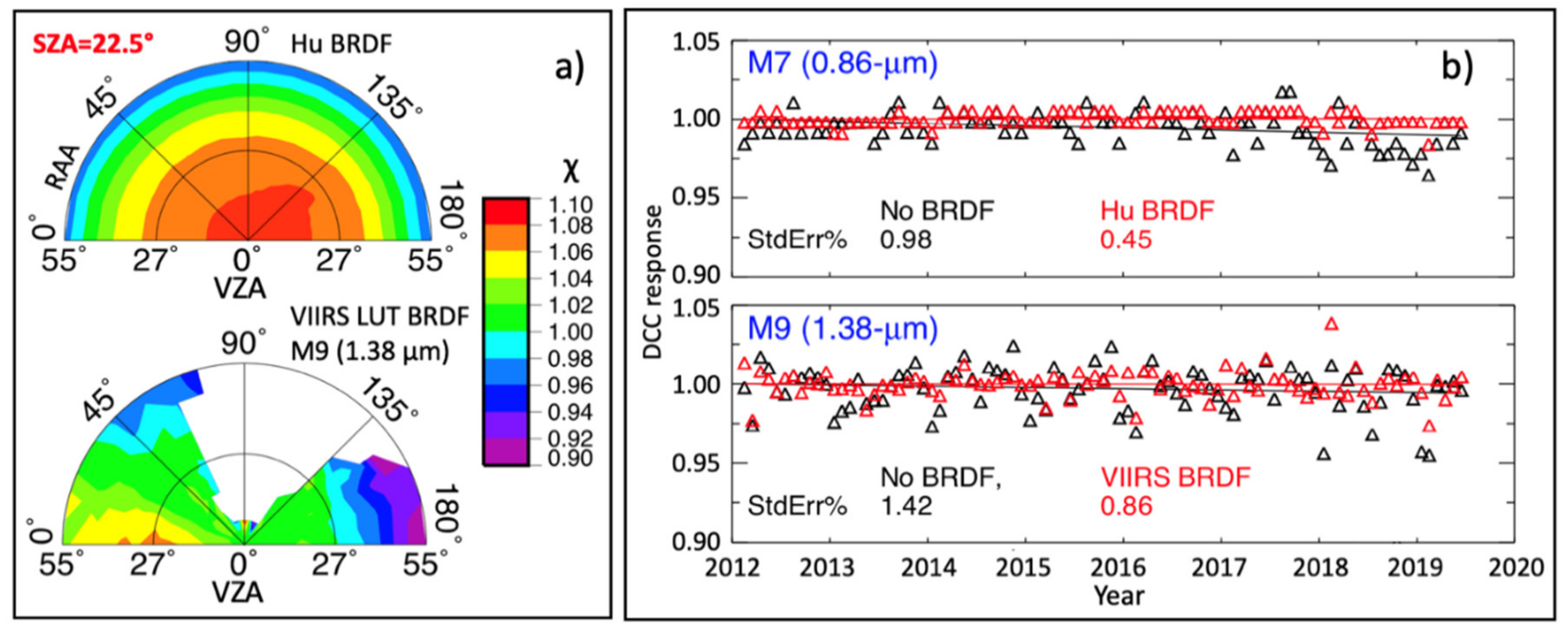
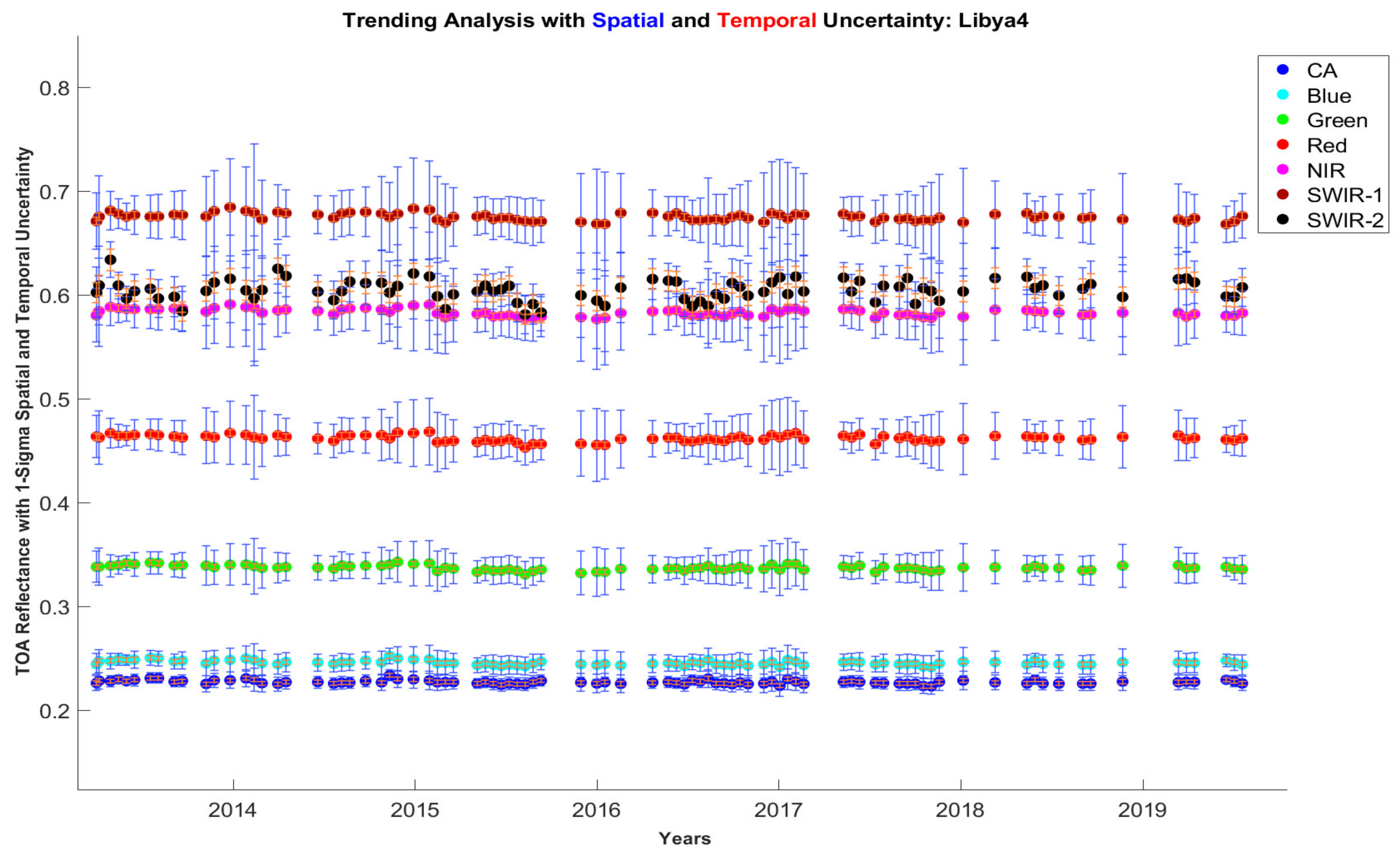
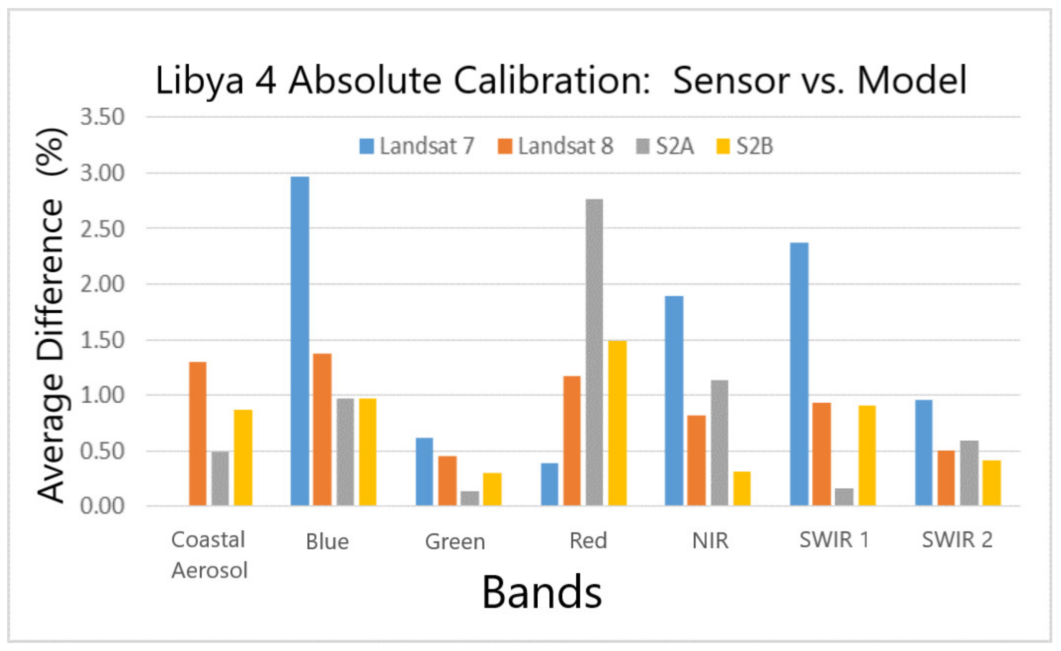
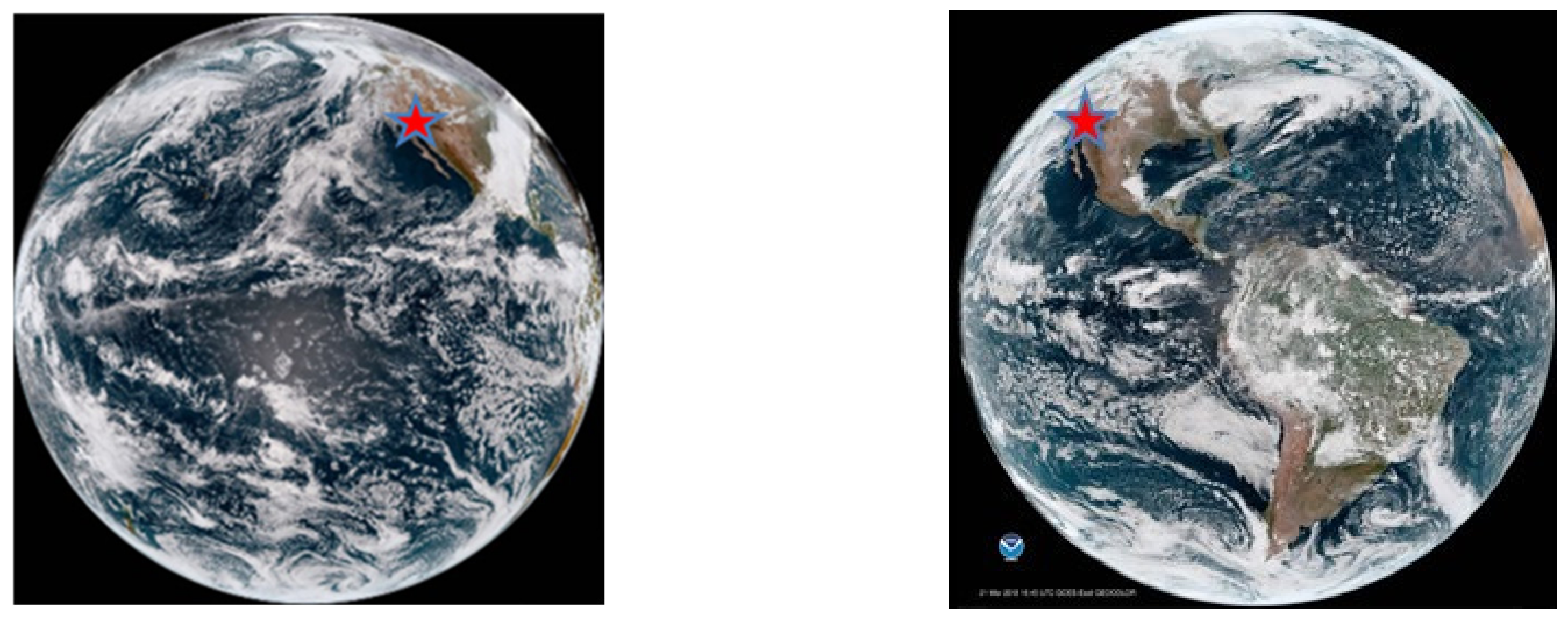
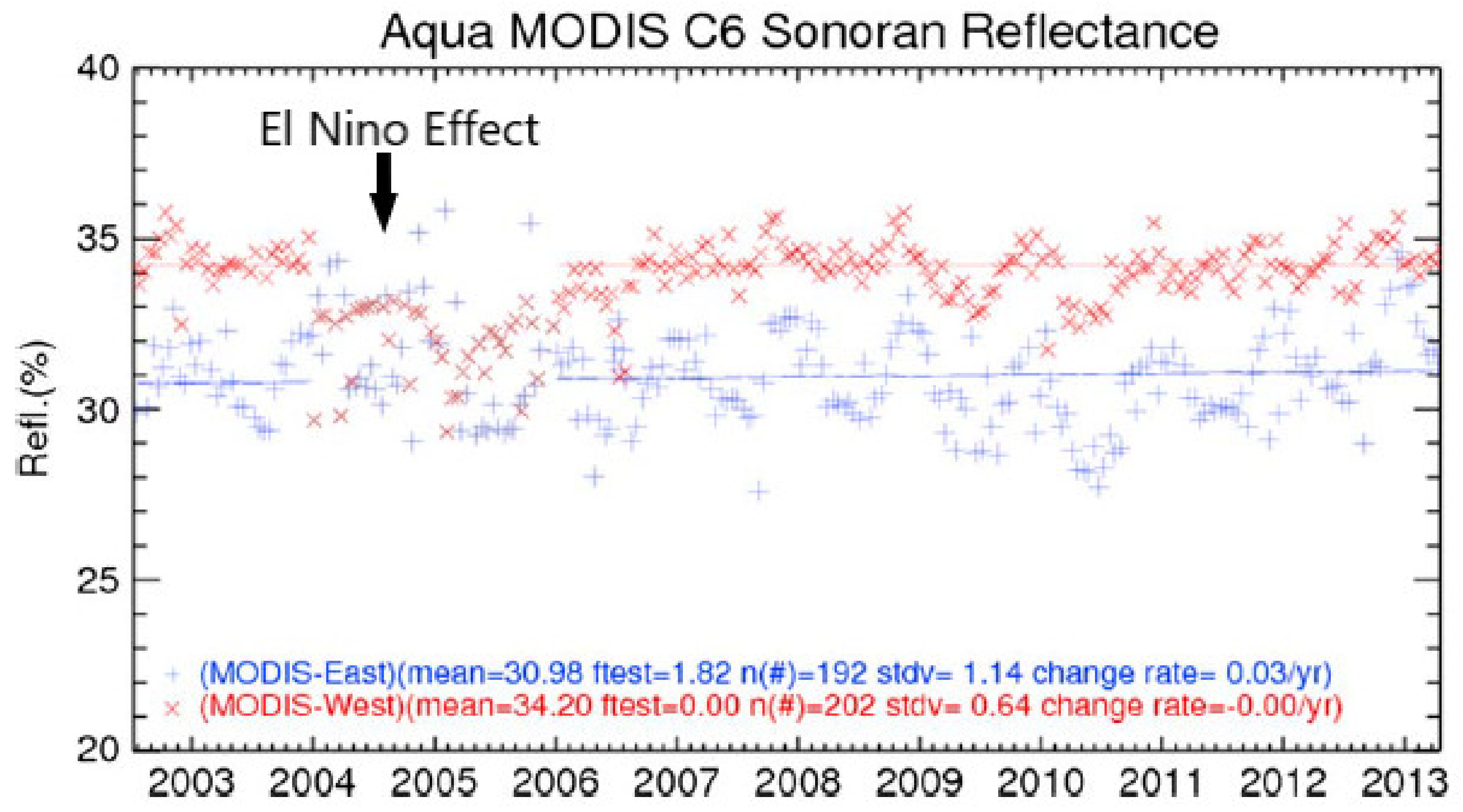
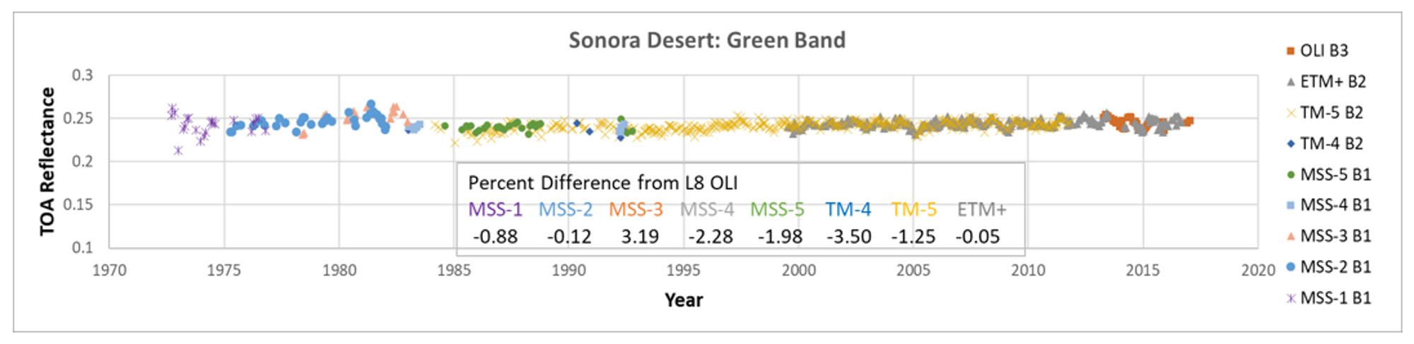
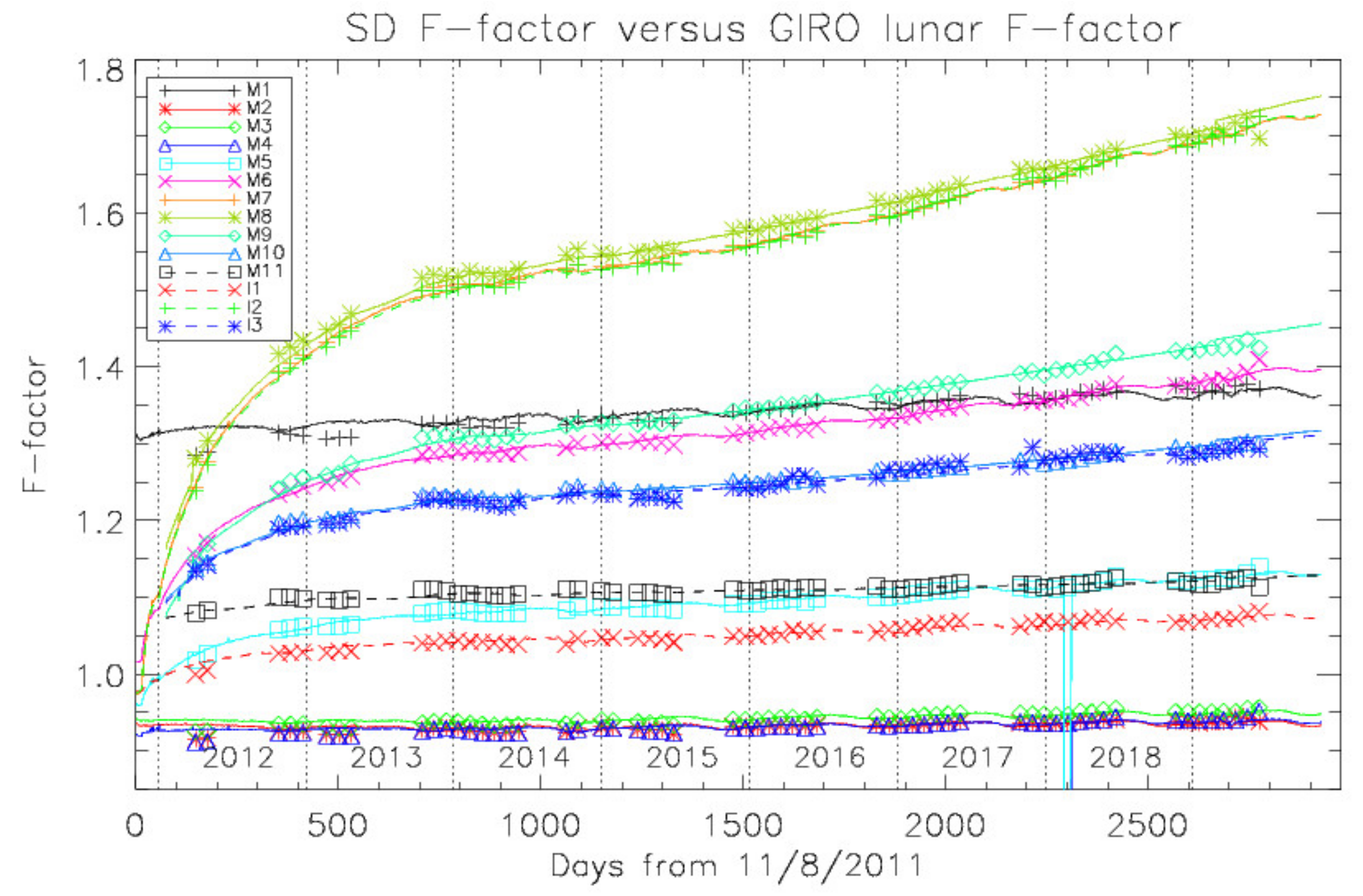
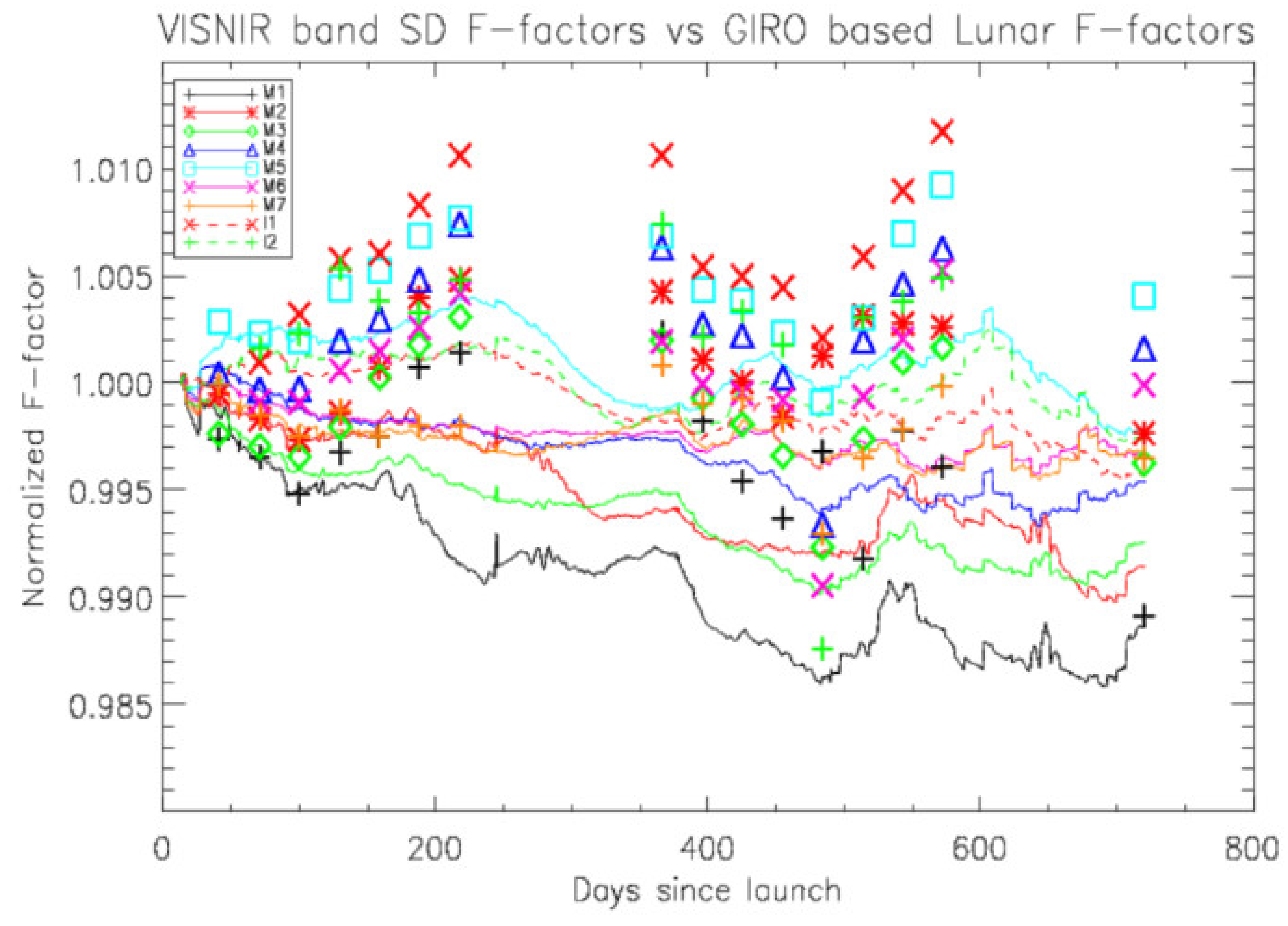
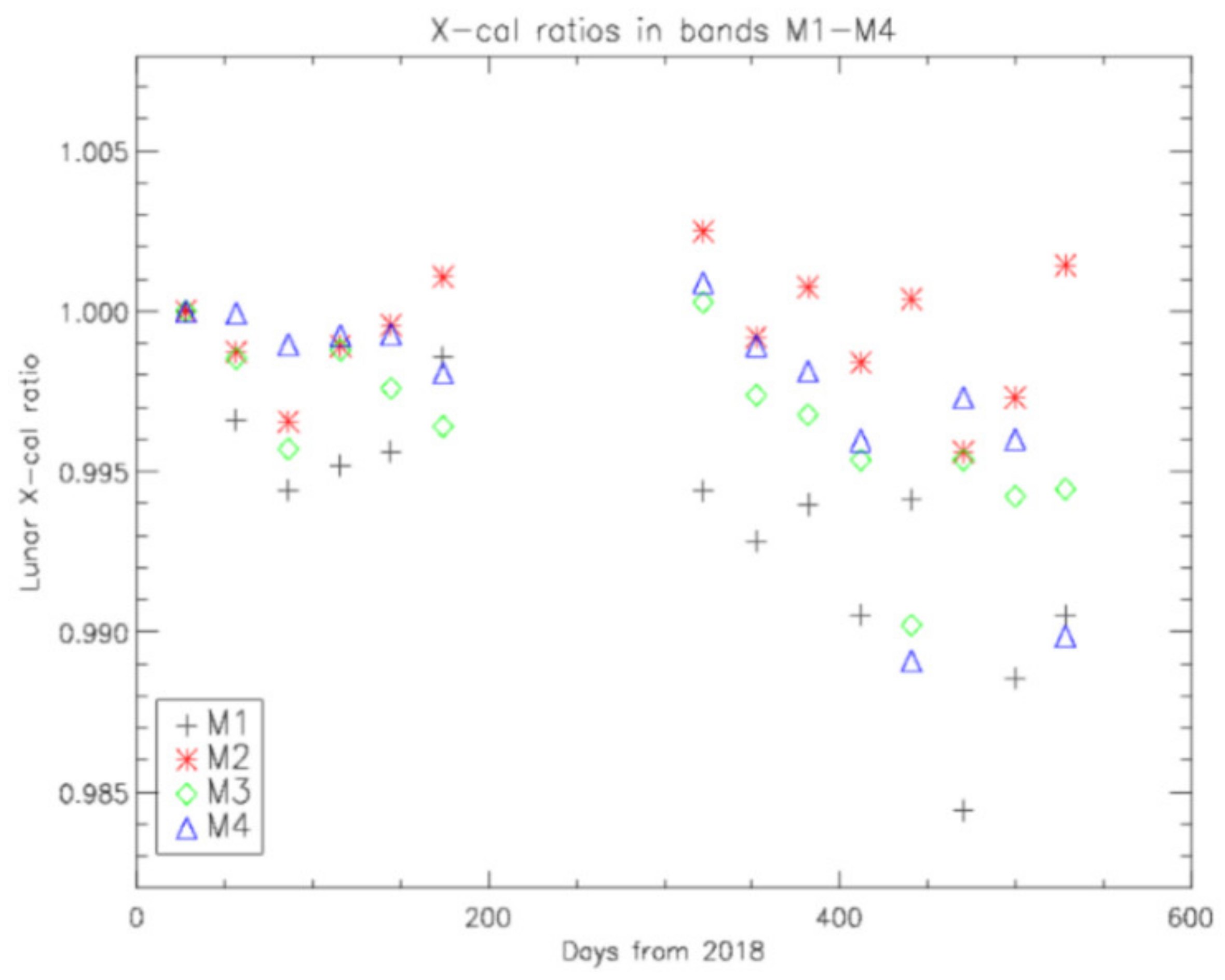
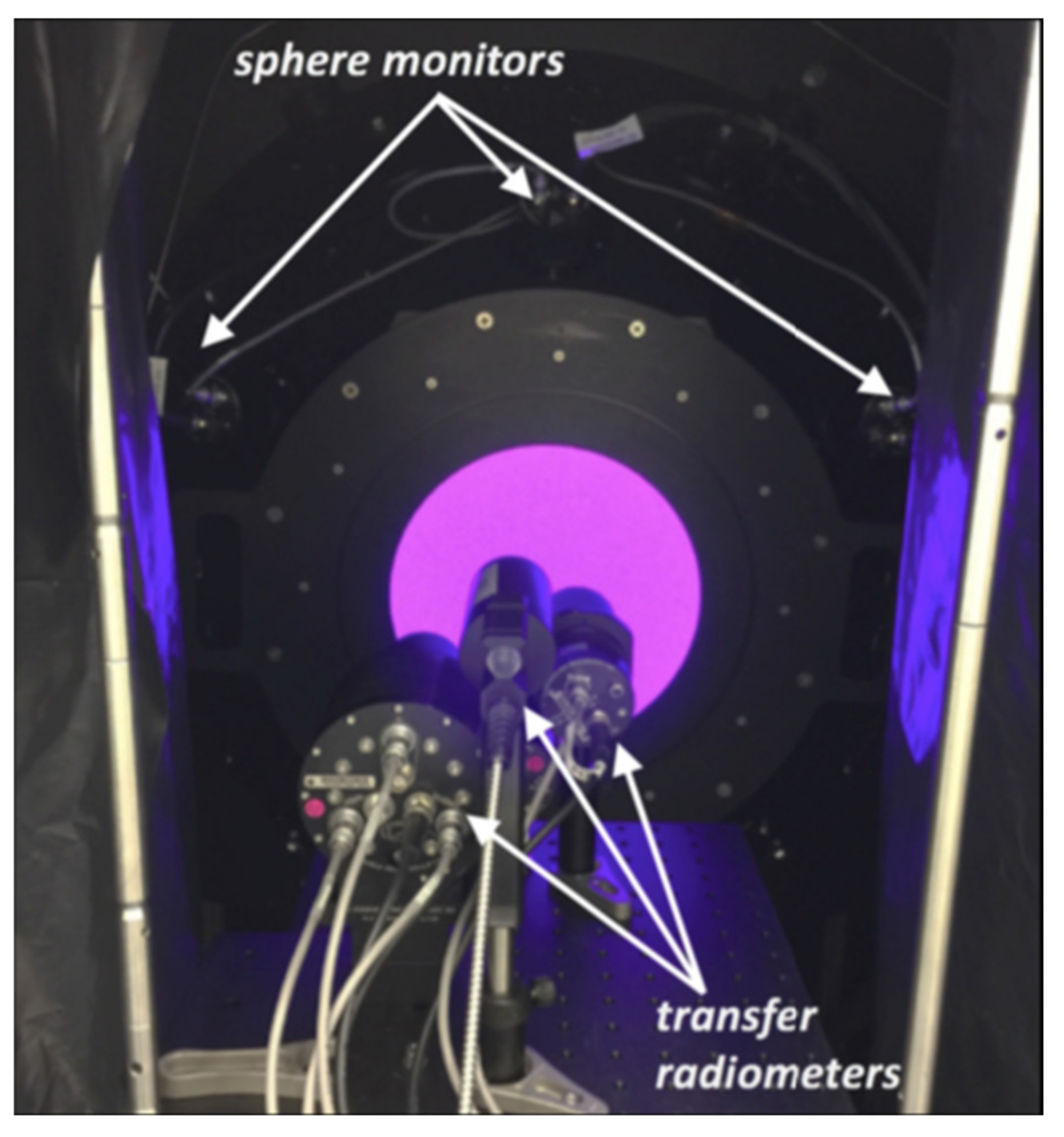
Table 1.
List of workshop panel members.
| Panel Member | Affiliation |
|---|---|
| Cody Anderson | U.S. Geological Survey, Earth Resources Observation and Science Center (USGS EROS) |
| Julia Barsi | Science Systems and Applications Incorporated (SSAI)/National Aeronautics and Space Administration Goddard Space Flight Center (NASA GSFC) |
| Rajendra Bhatt | SSAI/NASA Langley Research Center (LaRC) |
| Taeyoung Choi | Global Science and Technology/National Oceanic and Atmospheric Administration (NOAA) |
| David Doelling | NASA LaRC |
| Sirish Uprety | NOAA Affiliate |
| Xiangqian Wu | NOAA |
| FangFang Yu | NOAA Affiliate |
At the end of the workshop, panel members provided a list of recommendations for improvements in current calibration methods and new approaches to calibration. The rest of this paper is organized to first provide some background on the similarities and differences between sun-synchronous and geosynchronous optical sensor systems, followed by recommendations for improving current calibration capabilities, and then suggestions for new techniques for calibration. A set of summary and conclusion statements finishes the paper.
© 2020 by the authors. Licensee MDPI, Basel, Switzerland. This article is an open access article distributed under the terms and conditions of the Creative Commons Attribution (CC BY) license (http://creativecommons.org/licenses/by/4.0/).
Share and Cite
MDPI and ACS Style
Helder, D.; Doelling, D.; Bhatt, R.; Choi, T.; Barsi, J. Calibrating Geosynchronous and Polar Orbiting Satellites: Sharing Best Practices. Remote Sens. 2020, 12, 2786. https://0-doi-org.brum.beds.ac.uk/10.3390/rs12172786
AMA Style
Helder D, Doelling D, Bhatt R, Choi T, Barsi J. Calibrating Geosynchronous and Polar Orbiting Satellites: Sharing Best Practices. Remote Sensing. 2020; 12(17):2786. https://0-doi-org.brum.beds.ac.uk/10.3390/rs12172786
Chicago/Turabian StyleHelder, Dennis, David Doelling, Rajendra Bhatt, Taeyoung Choi, and Julia Barsi. 2020. "Calibrating Geosynchronous and Polar Orbiting Satellites: Sharing Best Practices" Remote Sensing 12, no. 17: 2786. https://0-doi-org.brum.beds.ac.uk/10.3390/rs12172786
Note that from the first issue of 2016, this journal uses article numbers instead of page numbers. See further details here.