Article

Harmonizing the Landsat Ground Reference with the Sentinel-2 Global Reference Image Using Space-Based Bundle Adjustment

by
Rajagopalan Rengarajan
1,*,
James C. Storey
1 and
Michael J. Choate
2
1
KBR, Sioux Falls, SD 57030, USA
2
U.S. Geological Survey, Earth Resources Observation and Science Center, Sioux Falls, SD 57030, USA
*
Author to whom correspondence should be addressed.
Remote Sens. 2020, 12(19), 3132; https://0-doi-org.brum.beds.ac.uk/10.3390/rs12193132
Submission received: 3 August 2020 / Revised: 18 September 2020 / Accepted: 20 September 2020 / Published: 24 September 2020
(This article belongs to the Special Issue Cross-Calibration and Interoperability of Remote Sensing Instruments)

Abstract

:
There is an ever-increasing need to use an accurate and consistent geometric ground reference in the processing of remotely sensed data products, as this reduces the burden on the end-users to account for the differences between the data products from different missions. In this regard, the U.S. Geological Survey (USGS) initiated an effort to harmonize the Landsat ground reference with the Sentinel-2 Global Reference Image (GRI) to improve the co-registration between the data products of the two global medium-resolution missions. In this paper, we discuss the process, results, and the improvements expected from this harmonization of two ground references using space-triangulation-based bundle adjustment techniques. The ground coordinates of the Landsat reference library, consisting of five million Ground Control Points (GCPs) were adjusted in a series of four simultaneous bundle block adjustments using thousands of Landsat-8 (L8) scenes anchored with more than 300,000 control points extracted from the GRI dataset. The net adjustments to each of the four blocks, namely, Australia, Americas, Eurasia, and Islands, varied anywhere from 1 to 13 m, depending on the accuracy of the GCPs in these blocks. The use of the GRI dataset in our bundle adjustment not only improved the absolute accuracy of the Landsat ground reference, but will also improve the co-registration between Sentinel-2 and Landsat terrain corrected products, as the European Space Agency plans to process the Sentinel-2 products using the GRI dataset. Independent validation of the Landsat products processed using harmonized GCPs with the GRI dataset indicated a global misregistration error of less than 8 m Circular Error Probable at 90 % (CE90), an improvement from the 25 m prior to harmonization. The improvements to the Landsat products using the harmonized GCPs are expected to be available to the public as part of Landsat Collection-2 processing by the end of 2020.

Graphical Abstract

1. Introduction

The increasing availability of moderate-resolution remote sensing data from a variety of sources at little to no cost to the user has made the assembly of dense time-series datasets ever more practical to support a wide range of applications, including global climate change studies, water management, monitoring land cover change, agriculture and forest management, homeland security, and disaster management [1,2,3,4,5]. Implicit in the ability to create and utilize these multi-sensor time series is the ability to register these data to a common geometric reference. A particular example of the benefits of using multi-sensor data for purposes of multi-temporal analysis is the interoperable use of the multispectral datasets acquired by the Sentinel-2 (S2) and Landsat families of sensors. Although the S2 and Landsat missions create products that nominally use the same geodetic reference system and map projection, differences in the geometric reference data used to create these products lead to residual misregistration between S2 and Landsat data products [6]. This residual misregistration places the burden of checking and, if necessary, refining the S2-Landsat registration on the user. This paper describes an effort to remedy this situation by improving the consistency of the S2 and Landsat geometric reference data.
Modern remote sensing systems, such as S2 and the current-generation Landsat-8, achieve highly accurate geolocation using data from satellite positioning systems (e.g., GPS) and onboard star sensors. Using these methods, accuracy at the pixel level is possible without the use of ground reference data [7,8]. Unfortunately, this level of accuracy is not sufficient for many applications that require multi-temporal data registration. In order to achieve multi-temporal registration accuracy, since the early 2000s, the Landsat archive, which includes datasets dating from the 1970s with widely varying inherent geometric accuracy, has used a global control point library based upon the Global Land Survey (GLS) circa 2000 dataset (GLS2000) [9] as a reference for Level 1 terrain-corrected products from all Landsat missions [8]. This control point reference set, which is publicly available via the Landsat website, ensured consistent registration across Landsat products, but was of limited accuracy in some areas, and is in need of modernization. Similarly, the S2 mission has created a Global Reference Image (GRI) using substantially cloud-free S2 Multispectral Imager (MSI) images linked together using a global triangulation procedure [10]. This GRI will be used as a common geometric reference for S2 data products to ensure consistency. The recent availability of the S2 GRI and the desire to modernize the Landsat control point library led to the effort, described here, to harmonize these two geometric reference datasets, thereby enabling substantially improved registration accuracy for S2 and Landsat products.
The method used to achieve the harmonization of the S2 and Landsat references uses Landsat-8 data in a space-based triangulation procedure, which has been described in detail elsewhere [11]. The ground coordinates of over five million Landsat Ground Control Points (GCPs) were adjusted in a series of four simultaneous bundle adjustments that each used hundreds to thousands of Landsat-8 scenes anchored with control points extracted from the S2 GRI, with supplemental control from the Australian Geographic Reference Image (AGRI). The feasibility of applying this triangulation approach at the continental scale was demonstrated for Australia prior to the Collection-1 reprocessing of the Landsat archive [11]. As a result of the current global readjustment, the Landsat GCP library will be made geometrically consistent with the S2 GRI, leading to Landsat data products with much-improved registration accuracy when compared with S2 products that have been aligned with the GRI. This improved registration accuracy will be realized by implementing the readjusted control for the Collection-2 Landsat archive reprocessing campaign.
The remainder of this paper describes the data used in the triangulation process, the geometry of the four triangulation blocks used to perform the global adjustment, the outputs of the triangulation processes, and the results of the validation techniques used to assess the performance of the triangulation and to predict the Landsat–Sentinel registration accuracy to be expected in the future.

2. Dataset

Our work is focused on improving the location of the ground coordinates of the GCPs that are used to produce Landsat orthorectified products. This improvement was achieved by measuring the apparent locations of these GCPs in Landsat 8 imagery and performing continental-sized block triangulation adjustments of the Landsat 8 data to refine the GCP positions. In this section, we provide a brief background on the datasets and the design of the block geometry used in our process.

2.1. Triangulation Block

The bundle adjustment using the space-based triangulation method described in [11] takes observations of GCPs from several scenes and iteratively solves them using the least-squares approach. The solution in our implementation requires an inversion of large matrices, which restricts how large an area can be or the number of scenes that can be solved together. Hence, we divided the global landmass into four individual sections or blocks. Since each block is solved independently, the design of the block must take into account how the blocks are split across the continents, as it can result in inconsistent adjustments at the block boundaries. In this study, the blocks were divided along the ocean–land boundaries into four large blocks, as shown in Figure 1. Solving large blocks, as shown in Figure 1, improves consistency across the entire block. The North American and South American continents were combined into a single block, referred to as the “Americas” block in this study. Similarly, Africa, Asia, and Europe are interconnected by land and, therefore, were combined into a single block, referred to as the “Eurasia” block. The Australian continent is disconnected from the rest of the continents and, therefore, was solved independently as a block. All the other islands and regions disconnected from the above three blocks were solved together in a single “Island” block.

2.2. Collection-1 GCPs

The GCPs used in Collection-1 were extracted from the GLS dataset constructed from Landsat 7 data circa 2000. The GLS datasets are decadal global mosaics of cloud-free orthorectified data that were generated from Landsat data that have been registered to the GLS2000 layer. The GLS2000 data were generated from Landsat 7 Scan Line Corrector (SLC)-On scenes after several independent studies revealed poor geometric accuracy of the predecessor GeoCover 2000 data [12,13]. The Landsat 7 scenes that were used to generate the GLS2000 dataset were processed using the Shuttle Radar Topographic Mission (SRTM) Digital Elevation Model (DEM), additional ground control, and Landsat 7 definitive ephemeris using a block triangulation process developed by MDA Federal Inc., USA (Maxar Technologies) [14]. Validation of GLS2000 data shows that absolute accuracy is better than 25 m Root Mean Square Error (RMSE) for most regions [15]. However, internal studies showed that certain regions were inaccurate by more than 50 m RMSE. This is especially true in places where accurate ground control positions were unavailable when the GLS was created [15]. Some of these regions were identified and updated prior to Collection-1 using Landsat 8 data with a space-based bundle adjustment technique. The Collection-1 GLS GCPs are small image chips of 64 × 64 pixels, centered at well-defined points of interest extracted from the GLS2000 dataset using an interest operator method [16] for Collection-1 processing.

2.3. GRI Dataset

Since the launch of the Sentinel-2 satellites, the European Space Agency (ESA) has been producing terrain-corrected products without the use of GCPs in their product generation system. The Sentinel-2 product’s geolocation accuracy was estimated to be better than 20 m (3 sigma) when no controls were used in the refinement of the geometric models [10]. Although the absolute pointing knowledge and geolocation accuracy of the Sentinel-2 satellites are better than most other remote sensing systems, the temporal misregistration requirement of 3 m for 10 m spectral bands could not be achieved without further geometric refinement. To improve and meet the multi-temporal registration requirement of the Sentinel-2 products, the ESA produced a ground reference, referred to as the Global Reference Image (GRI). The GRI can be defined as “a set of as cloud-free as possible” mono-spectral (red band at 10 m resolution) Level 1B (L1B) products, whose geometrical model has been refined through a dedicated bundle block adjustment process designed by the IGN (Institut Géographique National) with an objective of good and consistent geolocation [10,17]. The bundle adjustment process is based on a large space-triangulation that leverages the overlap between Sentinel orbits, tie points, and GCPs to improve the geometric model of the Sentinel 2 scenes [17]. The Centre National D’Etudes Spatiales (CNES) validated the accuracy of the GRI dataset using the Pleiades High-Resolution Database, which includes more than 500 images with an accuracy of less than 5 m. Their validation results show that the GRI dataset is accurate to better than 9.5 m Circular Error at 95% probability (CE95) [17].
The GRI dataset consists of one or more images per product tile, depending on the cloud cover. The GRI dataset was stored in the native image geometry (L1B product) and could not be used in our bundle adjustment process directly. Therefore, we requested and the ESA graciously provided a version of the GRI images that had been processed and projected to Level 1C (L1C) Universal Transverse Mercator (UTM) product tiles. Each GRI single-band image was provided in JPEG2000 format, which was resampled to 15 m using the Geospatial Data Abstraction Library (GDAL) toolkit to match the highest-resolution Landsat 8 band (panchromatic). Details on how the resampled GRI tiles were used in the harmonization process are provided in Section 3.3 and Section 3.4. A few of the requested tiles were not delivered (no usable data available or could not be processed at the time of request) or were covered with clouds, making them unsuitable for our harmonization process. For these cases, we used the Sentinel-2 L1C products that were terrain corrected but not adjusted by GRI or any other ground control. These scenes are referred to as “MSI Control” or “MSI Validation” scenes in this paper. To average out the date-to-date pointing variations with the MSI Control scenes, we chose three or more MSI products for each tile. To account for the poorer geodetic accuracy of the MSI Control scenes (in comparison with products processed using GRI), GCPs extracted from these products were provided with different a priori weights (lower weights) than the GCPs extracted from the GRI tiles.
In total, we received 3195 unique GRI images covering 1020 distinct geographic locations or tiles. Among the 1020 GRI tiles, about half of them (474 tiles) were used as control tiles in the bundle adjustment process, and the remaining tiles were used only to validate the corrections. The control tiles were chosen such that they were geographically well distributed in each block. A few control tiles were also added to regions where two large landmasses or continents are connected. This is important, as the distribution of the control tiles adds strength to the block geometry. In places where we determined a need for control, but the GRI tiles were unavailable, Sentinel-2 L1C products were used as control tiles (MSI Control). The validation tiles were chosen so that they were well distributed within the block and were not very close to the control tiles. As in the case with control tiles, a few MSI Validation tiles were chosen to validate the corrections from the triangulation process where GRI tiles were unavailable. Table 1 shows the number of GRI and MSI tiles used in each of the triangulation blocks, and the distribution of these tiles is shown in Figure 2.
One of the regions where the GLS GCPs were reworked prior to Collection-1 was in Australia. This was done to both improve the consistency of the GLS GCPs with the AGRI [18], the national geographic reference preferred by GeoScience Australia, and to demonstrate the feasibility of performing such adjustments on a continental scale. In this case, control points were extracted from the panchromatic AGRI dataset and then used to constrain the adjustment of the GLS GCPs [11]. To ensure that consistency with the AGRI was maintained through the readjustment for Collection-2, these AGRI control points were retained in the adjustment of the Australia block, so that the triangulation block contained both GRI and AGRI controls.

3. Methods

The Global Reference Image (GRI) dataset was used to improve the ground position of the Collection-1 GCPs using a triangulation-based bundle adjustment technique that was published in this special issue [11]. In this section, we provide only a brief introduction to the bundle adjustment technique; interested readers can use the cited article in [11] for detailed construction and implementation of this algorithm.

3.1. Bundle Adjustment Algorithm

The space-based triangulation method involves adjusting the spacecraft position, velocity, attitude, attitude rate corrections, and GCP coordinates iteratively so that the residual errors measured in the Landsat 8 images for the corresponding points are minimized. The observation equation or the look-point equation is non-linear and relates the ephemeris, attitude, and GCP to the image observation. Taylor series approximation linearizes the non-linear observation equation by computing the partial derivatives numerically. Using an initial approximation, a priori covariance information, and partial derivatives, a solution to the linearized equation was determined iteratively. Each iteration provides a set of incremental correction parameters. As the iterative solution converges, the incremental adjustments computed in each iteration grow progressively smaller. The iterations are halted when the adjustments to the parameters are smaller than a specified convergence threshold. The correction estimates for the parameters from each iteration are accumulated over all the iterations to provide the final adjustments for each of the parameters. In essence, the method solves a non-linear least-squares problem using a priori knowledge of the spacecraft and GCPs to minimize the residual errors from image-based observations of the GCPs. The mathematical formulation and description of our method are described in [11]. The details on how the data were gathered are discussed in the rest of this section.

3.2. GRI Harmonization Procedure

A simplified flow diagram of the triangulation process is shown in Figure 3. Although there were more than 2.5 million GLS GCPs distributed globally in the Collection-1 GCP database, these GCPs were generated from Landsat 7 SLC-On data, acquired between 1999 and 2003. To improve the temporal consistency and registration performance of the Landsat data, additional GCPs were extracted from the Landsat 8 L1T products using the interest operator algorithm [16] for all World Reference System (WRS)-2 path/row locations that contain land. The main advantage of using the interest operator algorithm for GCP extraction is that these GCPs are time-invariant and have a very high probability of correlation. The newly generated GCPs from Landsat 8 images were included in the bundle adjustment procedure, as these GCPs will also be used in the Collection-2 processing of Landsat data. For the AGRI images, evenly spaced image locations were identified for GCP extraction, as these GCPs will not be used to generate terrain-corrected products in the Landsat product generation system. Since the ground locations in the Landsat GCPs (GLS2000 or newly added Landsat 8 GCPs) were highly likely to correlate, as they were chosen using the interest operator, we decided to use the same locations to extract the GCPs (image chips) from the GRI tiles. Although the AGRI and GRI GCPs are similar to the Landsat GCPs, both in format and data structure, the AGRI and GRI GCPs were used only in the harmonization (bundle adjustment) process and will not be used in the Landsat product generation system.
The triangulation process begins with the identification of the Landsat 8 scenes that will be used to generate observations for the bundle adjustment. The entire Landsat archive is stored in the U.S. Geological Survey (USGS) Earth Resources Observation and Science (EROS) Center, where both the acquired images and corresponding ancillary information are available. The objective was to generate as many observations of the GCPs as possible for bundle adjustment. Therefore, cloud-free Landsat 8 scenes that were used to generate GCPs for each land path/row were chosen. These were not only cloud-free scenes, but also had the highest chance of correlation, as the Landsat Operational Land Imager (OLI) GCP image chips were generated from these scenes. As mentioned earlier, the bundle adjustment algorithm requires spacecraft information, such as ephemeris and attitude, GCP coordinates, and corresponding image coordinates, which were gathered through the precision correction process. A simplified process flow of the precision correction process is shown in Figure 4. The covariance information and the precision information are then used in the bundle adjustment technique to estimate the adjusted coordinates for the GCPs. Note that the bundle adjustment process provides adjustments to the ephemeris, attitude, and GCP coordinates, but we were only interested in the adjustments to the GCPs, as the main purpose of our study was to improve and harmonize our ground reference data (GCPs) with the GRI dataset.

3.3. Precision Correction Process

The overall process of generating a Landsat terrain-corrected product is shown in Figure 4. The scene selection process is not part of the standard terrain correction process, but in this analysis, only selected scenes that matched the cloud cover and GCP correlation success criteria were chosen. The ephemeris and attitude data measured by the spacecraft for each acquisition are contained in the ancillary file. The ancillary data and the calibration parameters (Calibration Parameter File (CPF)) are used to generate the line-of-sight (LOS) model (systematic model) of the OLI sensor. The raw (radiometrically uncorrected) scene’s detector response was normalized by adjusting for the detector’s relative and absolute gains to generate a radiometrically corrected Level 1R (L1R) product. Note that the radiometric correction also includes other calibration and correction procedures, such as non-linearity, saturation, etc. The systematic model and the DEM are used to geometrically correct the L1R image for sensor acquisition and viewing geometry effects to generate the systematically terrain-corrected product (L1GT).
As noted, the GCPs for Collection-1 were generated from the Global Land Survey (GLS2000) dataset. The GLS2000 dataset provides global coverage of the orthorectified product, but the geopositional accuracy in some regions was worse than 50 m. These isolated regions were identified and corrected using Landsat 8 data and the triangulation-based bundle adjustment technique described in [11]. The majority of the suspect regions were cleaned up before Collection-1 processing, resulting in a net RMSE of 25 m [6,15]. Although the absolute accuracy of the Collection-1 GCPs is worse than the absolute geodetic accuracy of Landsat 8 data [8], all the Landsat (Landsat 1 through Landsat 8) orthorectified products are precision corrected (corrected using GCPs) to ensure scene-to-scene temporal consistency across the Landsat archive. The location of GCPs in the L1GT image is measured in the GCP mensuration process, which uses normalized gray-scale correlation techniques to match the Shortwave Infrared (SWIR)-1 (band 6) image of the OLI sensor with the GCPs stored as image chips in the Collection 1 GCP database. The correlated and measured GCPs are then used to estimate the orbit and attitude adjustments to the systematic model in the precision model fit procedure. The precision model, DEM, and the L1R image are then used in the image resampling process to generate the Level-1 terrain-corrected product (L1T).
What we have provided so far is a brief process flow of the Landsat 8 terrain-correction process. It is beyond the scope of this article to discuss each algorithm/process described in Figure 4 in any detail. For a detailed description, readers are encouraged to look at the Landsat Algorithm Description Document [19]. Note that in a typical L1T generation process, orthorectified image products are generated for all of the Landsat 8 bands, but in our analysis, we are only interested in the GCP measurements, and, therefore, band 6 alone is processed and used. The shaded (transparent blue) part of the flowchart in Figure 4 shows the precision correction process, which is used to generate observation equations for the bundle adjustment procedure. The important information provided by the precision correction algorithm is discussed briefly in the next Section 3.4.

3.4. Extraction of Observations

The precision correction algorithm shown in Figure 4 uses the results from GCP measurements in an L1GT image that was systematically terrain-corrected using the original LOS model to derive estimates for corrections to the systematic LOS model. Corrections to the spacecraft attitude and ephemeris are computed in a least-squares procedure, which minimizes the differences between the measured locations of the control points and their true ground locations. This procedure includes the detection and removal of outlier GCPs using a modified t-distribution test. These corrections are added to the LOS model to create a “precision” model for subsequent use by other geometric algorithms. The precision model is verified by checking for simple threshold tests, such as RMSE of the pre-fit and post-fit GCP measurement residuals, the number of points declared as outliers, etc., before being accepted as a successful precision model solution. The output from the precision solution process includes the following for each inlier GCP: geodetic coordinates of the GCP from the GCP database, image location of the corresponding GCP, coordinates of the GCP point as measured in the systematic image (L1GT), the time when the GCP was imaged (GCP time), ephemeris position, ephemeris rate (velocity), attitude, and attitude rate at the GCP time of observation. Thus, for each observation point kept in precision correction, we record the observation vector (LOS vector of the GCP), time of observation, spacecraft position and velocity, and spacecraft attitude and attitude rate.
The standard deviations used to determine the weights or a priori covariance in this study for the observation point, ground point, spacecraft position, and orientation are shown in Table 2. Note that the a priori weights vary depending on the accuracy of the GCPs. In our study, we constrained the adjustments to the GCP coordinates by providing large weights (small Standard Deviation (STD)) to the GRI and AGRI control points, which will provide stability and make GLS GCPs harmonized with the GRI dataset. Although the 10,000 m standard deviation attributed to the Collection-1 GLS GCP positions does not reflect the accuracy of individual GLS GCPs, it was necessary to use a large a priori standard deviation to prevent the GLS GCPs from overly influencing the solution, especially when more than 1000 GLS GCPs are measured in an image. The main objective of our work is to harmonize our ground reference (GCPs) with the GRI dataset, and therefore, the GRI GCPs were provided with a 5 m a priori standard deviation. During the development of the GRI dataset, the IGN used the AGRI dataset to constrain its solution over Australia. Hence, the AGRI and GRI GCPs were provided with the same a priori weights. The a priori standard deviation for MSI GCPs was chosen to be 10 m, as it is consistent with the geolocation uncertainty of the MSI L1C products, which, in general, are better than 11 m CE95 [20]. We used the SRTM data as the vertical reference, while the AGRI and GRI GCPs are used as a horizontal reference for the GCPs. The SRTM dataset, in general, is better than 30 m in its vertical accuracy, and therefore, the a priori standard deviation for the height coordinate was set to 30 m [21,22].
The Landsat 8 spacecraft uses highly accurate GPS and attitude sensors for its position and orientation estimates, respectively. This allowed us to use a small a priori standard deviation of 4 m for the position, 1 mm per sec for velocity, and 10 micro-radians for the orientations. The a priori covariance estimates for the AGRI and GRI GCPs, ephemeris, and attitude were chosen to be small so that the corrections were predominantly in the GLS GCPs, thereby transferring the accuracy of the GRI and AGRI GCPs to the GLS GCPs. Furthermore, the a priori estimates for attitude and ephemeris were consistent with the established pointing accuracy of the Landsat 8 (L8) based upon on-orbit characterization [8]. Although well-defined points (GCPs) can be correlated with the images to better than a tenth of a pixel, for image observation a priori estimates, we chose 5 m as the a priori standard deviation to account for any unknown correlation-related errors. As discussed in the triangulation method [11], the initial approximations and their corresponding covariance information were used as input to the bundle adjustment to estimate the adjustments for each of the parameters.
The bundle adjustment algorithm was implemented in the C programming language with four files representing pass, image, ground, and observation as input. As an example, a record for each of the four input files is shown in Table 3. The pass file contains a priori information for each pass used in the triangulation block. A pass consists of an entire descending orbit (acquired on the same day) and may contain one or more images, which need not be contiguous. The triangulation solution provides one correction per pass for the spacecraft’s position and velocity; therefore, the pass file contains as many records as there are unique passes in the block. The image file contains a priori weights for each WRS-2 scene used in the triangulation block. The images are linked to the spacecraft’s position and velocity by the pass identifier. The triangulation solution provides one set of corrections (for attitude and attitude rate) per image. The observation file contains all the observation-related information, such as the spacecraft’s position and velocity for the given observation point, the LOS vector of the observation, the a priori weights for the image observation, and the partial derivatives of the LOS vector. The ground file contains coordinate and a priori information about the GCPs observed in the image. The triangulation solution provides one set of corrections to each ground point. The ground points are identified by a unique GCP identifier (ID), which is used to link the ground point with the corresponding observations in the observation file. Note that the observation file may contain more than one observation per ground point, as the same GCP can be observed from multiple images.

3.5. Image-to-Image Registration

For validation, we estimated the geometric difference between the GRI dataset and Collection-2 Landsat L1T products using an image-to-image registration process. The image-to-image registration method provides an assessment of the geometric misregistration between the two images using a similarity measure, such as normalized cross-correlation. The method works by choosing locations within the reference image (Landsat L1T product) and search image (GRI tile), extracting windows (64 × 64 pixels) of imagery from each image, and performing gray-scale correlation on the image windows. Criteria such as measured displacement and strength of the correlation peaks are used to identify and remove bad correlations. The sub-pixel location of the measured offset is calculated by fitting a second-order polynomial around the correlation surface and solving for the fractional peak location of the fitted polynomial. The correlation and the sub-pixel estimation process are repeated for all the test points identified in the reference/search image. Finally, the t-distribution-based outlier rejection method is used to remove any outliers in the test point measurements. The statistics such as mean and standard deviation for the valid points provide an estimate of the misregistration between the two images. In our study, we performed this validation for all of the GRI tiles that were identified as validation tiles. For details on this procedure and its implementation, refer to the Landsat 8 Algorithm Description [19].

4. Results

The space-based triangulation method was used to perform a continent-level block triangulation over four major blocks. Each block includes all the WRS2 paths/rows that contain land features. Using the GRI dataset as a source for ground reference in the bundle adjustment procedure, we improved the absolute accuracy of the GCPs derived from the GLS2000 and OLI images. The GCPs extracted from the GRI images were provided with higher weights in comparison to the Collection-1 and OLI GCPs to constrain the adjustment of the block. Table 4 shows the number of observations, passes, images, and control points used in the bundle adjustment procedure for each block. For all the blocks, the triangulation algorithm converged to a solution in two iterations. The number of iterations and the RMS error of the observations before and after the bundle adjustment for each of the blocks is shown in Table 5. The bundle adjustment reduced the overall observation error by a factor of about 7, except for the Islands and Australia blocks. In the case of the Islands block, only 36 unique GRI control tiles were used for 387 island paths/rows. The weak geometry of the Islands block (poorly connected land paths/rows in the block) coupled with a relatively lower number of GRI control tiles caused the post-adjustment RMSE to be higher than other blocks. In the case of the Australia block, the post-adjustment RMSE is the lowest among all the blocks, but the error improvement factor reduced from about 7 to less than 5 because the Australia block was triangulated using the AGRI reference dataset prior to our GRI harmonization effort. As a result, the GLS GCPs over Australia were more accurate, resulting in lower RMSE prior to the bundle adjustment.
As part of the output, the triangulation algorithm provides for each GCP: the updated horizontal and vertical coordinates, the GCP residuals/position adjustment, and the number of images that observed the GCP. The number of observations for each GCP can be used to calculate an average number of observations per GCP for each WRS-2 Path/Row. This metric is an indicator of the strength of the block geometry, as the block strength increases when more observations are available per GCP. For example, if all the GCPs in a path/row were observed only once, then this path/row will be adjusted independently and will not be tied well with its neighbor. Although attitude correlation and pass correction should help to some extent, if there is more than one scene in this pass, most of the corrections to the GCPs will be dependent on the image position and orientation estimates, especially if highly accurate ground controls are unavailable for this path/row. Thus, the consistency within a block improves as the number of observations per GCP increases, which is dependent on the overlap between any two images in the block. For Landsat images, the overlap varies as a function of latitude, with the largest overlap near the poles (>70%) which reduces to the least (<10%) near the equator. Therefore, the majority of the interior GCPs in the tropical and temperate zones will be observed only once, unless images from a different date are used in the triangulation procedure. However, adding additional images to the block will increase the size of the block significantly, and will affect the ability to solve the large blocks used in this study. We resolved this practical issue by adding additional images only for those regions that were identified as suspects from our Landsat calibration studies or for isolated large islands where GRI controls were not available. Figure 5 shows the average number of observations per GCP for each path/row used in the block adjustment procedure. As expected, a large number of multipoint observations per GCP were observed in the northern latitudes, where the scene-to-scene overlap can be as high as 70%. Additional scenes were added to four suspect regions (two passes in Asia and two passes in South America) to account for geodetic uncertainties in these regions due to Landsat 8 calibration-related activities. Additional scenes were added to regions (southern part of Saudi Arabia, northeast and central part of the U.S., New Zealand, and a few other islands) to account for seasonal variations and cloud cover in the images used in the block.
The horizontal residuals for each GCP from the triangulation solution can be aggregated to compute an average offset in the latitude and longitude directions for each of the WRS-2 paths/rows used in the block adjustment. Figure 6 and Figure 7 show the mean residuals in the latitude and longitude directions, respectively, for each of the WRS-2 paths/rows used in the block adjustment procedure. The harmonization and improvement of the GCPs were assessed using two validation methods: (a) geodetic assessment procedure and (b) the image-to-image (I2I) characterization procedure described above. In the geodetic assessment procedure, the geodetic offsets of Landsat 8 scenes that were processed using spacecraft pointing knowledge and corrected for relief displacement were estimated using the updated GCPs. We used the precision correction procedure mentioned in Section 3.3 to process the L8 scenes, and the statistics from the precision correction process provided scene’s geodetic offsets. The advantage of this method is that geodetic offsets can be estimated globally for all the paths/rows where there are GCPs. Moreover, comparisons of geodetic offsets before and after the GCP updates provide both a measure of improvement in the GCPs and the differences that are to be expected between the Collection-1 and Collection-2 Landsat products. The results from the bundle adjustment procedure and the validation of the updates to the GCPs for each block are discussed in the rest of this section.

4.1. Australia

4.1.1. Triangulation Solution

As discussed earlier, the Australia block was small compared to all the other blocks, but was not small enough to be treated as part of the Islands block. Furthermore, GeoScience Australia provided AGRI reference images for Australia, which were used to adjust the GCPs over Australia prior to Collection-1. Therefore, we adjusted and validated Australia as an independent block. As shown in Table 4, 305,474 GCPs (286,115 GLS, 8,462 GRI, and 10,897 AGRI) were imaged in 405 L8 images that were acquired on 274 distinct passes to generate 581,706 observations. The GRI GCPs (GRI Control tiles) were well distributed, as is evident in Figure 2, and the MSI controls were not required for this block. Since the AGRI reference images were also used in the generation of GRI, we expected only a minor change to the positions of the GCPs in this block. The mean residual offsets after the triangulation for all the GCPs in this block were 0.61 and 0.81 m in the latitude and longitude directions, respectively. The corresponding STDs were 2 and 1.45 m, respectively. The small mean and STD for the entire block indicated a very small change in the GCP positions for this block, as expected. The mean and STD for a block are good indications of an overall change, but any isolated or large change is best observed from the plots. This was confirmed in Figure 6 and Figure 7, where the mean GCP residuals in the latitude and longitude directions were well below 6 m for all the paths/rows in the block. The small adjustments in the Australia block demonstrate that the addition of the GRI control did little to change the AGRI-based Collection-1 adjustment, thus showing the consistency between the GRI and AGRI datasets.

4.1.2. Geodetic Accuracy Validation

In this validation procedure, cloud-free L8 scenes were chosen for the GRI control and validation tile locations. The selected L8 scenes were processed in the Image Assessment System (IAS) to estimate the geodetic offsets using both the bundle-adjusted and the Collection-1 GCPs. Table 6 shows the mean geodetic accuracy for the Australia block using the control and validation scenes. The number of L8 scenes in this table is different from the number of GRI tiles shown in Table 1, as more than one L8 scene was processed in some cases for a given control or validation path/row. The column “Type” indicates whether the assessment was for control or validation tile locations. The “NUM SCENES” column shows the number of scenes evaluated. The geodetic accuracy procedure provides scene summary statistics that include mean and STD of the measured GCP residuals for each scene. The STD from the geodetic accuracy procedure is a measure of the scene’s internal geometric inconsistencies, which includes GCP-to-GCP variations. As confirmed in [8], pushbroom design and extensive calibration of the OLI sensor reduced the internal geometric inconsistencies significantly, and the majority of the variability measured will be due to the inconsistency between the GCPs. The mean across-track (XT) and mean along-track (AT) values in Table 6 were computed by taking the average of the mean geodetic offsets from the geodetic accuracy process in the across-track (XT) and along-track (AT) directions for all the scenes. Essentially, this is an average of the GCP residuals measured across all the GCPs for all the scenes in the block. The STD XT and STD AT were computed by taking the standard deviation of the mean geodetic offsets for all the scenes. These two metrics indicate the variability in the L8 pointing accuracy for the selected L8 scenes in the block. Therefore, for scenes processed with the updated GCPs, these numbers are expected to be in the same range as the established pointing accuracy of L8 based upon on-orbit characterization (18 m CE90) [8], if we assume the accuracy of the updated GCPs is similar to the accuracy of the geometric calibration sites. Note that the STD statistics were based on single-scene statistics for each path/row, whereas the on-orbit characterization results were estimated from hundreds of scenes over calibration sites. Therefore, the estimates in this table will not be an exact match to L8 pointing accuracy. The last two columns (Consistency XT and Consistency AT) were computed from the root mean square (RMS) of the STD (from the geodetic accuracy process) of all the scenes in the block. Since these two columns were based on the STD from the geodetic procedure, these columns provide a measure of the internal consistency of the GCPs within the block. Rows one and two in Table 6 show the results for the control scenes using the original Collection-1 GCPs and the Collection-1 GCPs after adjustment, respectively. Rows three and four show the same for the validation scenes. The last row shows the result for validation scenes that were processed using all the updated GCPs, including the newly generated GCPs from OLI images. Consistency between control and validation results would suggest that the GCP improvements are not confined to the control tiles, but are distributed across the entire block. Similarly, consistency between rows four and five suggests that the updates are similar for all the GCPs and are not dependent on the sources from which they were generated.
From Table 6, it is evident that the results are similar before and after bundle adjustment for both control and validation scenes, with minimal change in the GCPs’ position in this block. This is expected; as mentioned earlier, the Australia block was adjusted using the AGRI dataset prior to Collection-1.
Since the geodetic accuracy can be estimated for any scene in the IAS, we chose and processed one scene per land path/row (in the descending pass) using GCPs before and after the bundle adjustment. The results are summarized in Table 7. The main difference between the two tables is that Table 6 shows results for a smaller number of scenes, specific to GRI control and validation tile locations, whereas the results in Table 7 were based on all the path/row locations in the block. Consistency between the two tables for a given block suggests that the validation results are independent of where they were geographically located and the date on which the L8 scenes were acquired. Figure 8 and Figure 9 show the radial geodetic offsets for the scenes that were processed with GCPs before and after bundle adjustment. The table provides block-level summary statistics, whereas the figures provide an insight into where large offsets were measured.
As expected, the geodetic offsets of L8 scenes are similar before and after the GCP updates for the 404 scenes in this block, which are evident from the table and figures. Note that the means in both XT and AT directions are higher in Australia than in other blocks, while the STD and the consistency are lower. The 4 m mean offset in the XT direction was confirmed when we averaged all the Landsat 8 products over Australia in Collection-1, but in the AT direction, the average for all the products was reduced to −2 m. There are two possible explanations to this behavior. The first explanation is that there may have been a systematic bias of 4 m in XT and about 2 m in the AGRI ground reference dataset. Since the AGRI dataset was used by the ESA in their GRI generation process, the bias was probably carried into the GRI dataset as well. This is evident from the results using updated GCPs, which also show similar bias in the XT and AT directions. Another explanation is that a thermal-induced alignment variation in L8 spacecraft could have introduced a small alignment change between the focal plane and the navigation reference. This alignment change may have introduced a bias of 4 m in the XT and about 2 m in the AT directions for Australia. Any change in the alignment can be analyzed only from accurate and consistent ground controls all over the world, which were not available in Collection-1. The USGS CalVal team has plans to investigate the systematic offset over Australia using Collection-2 processed Landsat 8 products.
The explanation for lower standard deviation is probably that the Australia block, in addition to being a small block, is the most benign area with regard to snow/ice and extreme terrain compared to other blocks. As explained earlier, the lower consistency in the Collection-1 results was because the Collection-1 GCPs over Australia were improved using the AGRI dataset and, therefore, were geometrically consistent and better than the Collection-1 GCPs in other blocks.

4.1.3. Image-to-Image Validation

In this process, the Image-to-Image (I2I) characterization procedure was used to assess the geometric offsets between the GRI tiles and the L8 scenes processed using GCPs before and after the bundle adjustment. Unlike the geodetic accuracy procedure, this comparison directly provided an estimate on the absolute accuracy of the GLS GCPs in comparison with the GRI dataset. Table 8 shows the validation results for the Australia block using the GRI tiles and L8 L1T products that were processed using GCPs before and after bundle adjustment. For the 44 control tiles, the Radial Root Mean Square Error (RMSEr) between the GRI tiles and L1T products that were processed using Collection-1 (GLS) and bundle-adjusted GCPs was 4.78 and 3.46 m, respectively. The results were consistent with the validation tiles. Note that the differences between the pre- and post-GCP updates were small and were better with the GRI GCPs, as expected. These results are consistent with the validation results using the geodetic accuracy procedure.

4.2. Americas

4.2.1. Triangulation Solution

The Americas block includes both the North American and South American continents. The block consists of 1,694,468 GCPs that were imaged in 3636 L8 images, acquired on 1845 distinct passes to generate 5,029,280 observations. As can be observed in Figure 2, the GRI control tiles were well distributed, except in the Aleutian Islands (Alaska), where we had to use MSI control tiles. As mentioned earlier, we used an average of three MSI tiles for every path/row to average the scene-to-scene differences in the MSI (S2 L1C) products. The mean residual offsets after the triangulation process for all the GCPs in this block were 1.09 and –0.03 m, and the corresponding STDs were 10.67 and 11.48 m in the latitude and longitude directions, respectively. Although the mean and STD are good indications of the improvements, the large changes to the GCPs in the block are better observed for the individual paths/rows, which were evident in Figure 6 and Figure 7. Most of the large changes to the GCPs were observed in the South American continent, where the GLS dataset was not highly accurate.

4.2.2. Geodetic Accuracy Validation

Table 9 shows the mean geodetic accuracy for the Americas block using the control and validation scenes. For the 161 control scenes, the mean geodetic offsets in the XT and AT directions were small for both before and after the GCP updates. However, the STD of the geodetic offsets for these scenes was considerably smaller for the scenes processed with updated GCPs, which suggests that the estimation of the geodetic offsets for L8 improved significantly with the use of updated GCPs. Moreover, the consistency of the GCP-to-GCP differences in both directions was significantly smaller for scenes processed with the updated GCPs, which further validates the improvement achieved by the bundle adjustment procedure. The results for the 191 validation scenes were similar to the results for the control scenes, with a significant reduction in the STD and GCP-to-GCP variations. Note that the last row in Table 9 is similar to the validation results that only used GCPs that were used in Collection-1 (fourth row). This indicates that all the GCPs (newly generated from L8 and Collection-1 GCPs) were both accurate and internally consistent in this block. Comparing Table 7 and Table 9, it is evident that the results are consistent and independent of the geographical locations. From Figure 8 and Figure 9, it was observed that the overall geodetic offsets for all the path/rows in the block improved, as is evident from the low radial geodetic offsets in Figure 9. An interesting feature with large geodetic offsets can be observed, which were shown as white ellipses in Figure 9. The Landsat CalVal team verified that those large offsets were not in the GCPs but with the L8 scenes over those passes due to the effect of solar calibration, which affects the pointing knowledge of the L8 spacecraft for a short duration. This effect was also observed in the Collection-1 results, but the large variability within and between the scenes in the block masked the effect of the calibration event.

4.2.3. Image-to-Image Validation

Table 10 shows the validation results for the Americas block using the GRI tiles and L8 L1T products that were processed using Collection-1 (GLS) and bundle-adjusted GCPs. For the 472 control tiles, the RMSEr between the GRI tiles and L1T products processed using Collection-1 and adjusted GCPs was 14.82 and 5.04 m, respectively. Similar results were observed for the validation tiles, where the RMSEr improved from 16.33 to 4.59 m after the bundle adjustment with the GRI control tiles. As mentioned earlier, we also used a few MSI L1T products as controls, and these path/rows were validated with a different set of MSI L1T products. The RMSEr between the MSI and L8 L1T products were slightly worse than the GRI tiles for Collection-1 products (using GLS GCPs). However, the same L8 L1T products processed using bundle-adjusted GCPs were better with lower RMSEr. Note that the accuracy of the S2 MSI L1C products was expected to be worse than the GRI-processed products, as the MSI products were generated using only the S2 spacecraft pointing knowledge and were not corrected with GCPs. The significant reduction in the RMSEr in the I2I validation and the reduction of the L8 geodetic offset estimation using the bundle-adjusted GCPs demonstrate the significant improvement achieved with our bundle adjustment techniques.

4.3. Eurasia

4.3.1. Triangulation Solution

The Eurasia block includes all of Africa, Europe, and Asia. The block consists of 3,410,168 GCPs that were imaged in 5673 L8 images, acquired on 2993 distinct passes to generate 7,938,901 observations. In this block, we used GCPs from MSI L1C products where we did not have GRI tiles, and a few AGRI GCPs were used that overlapped with the Australia block. The mean residual offsets for all the GCPs in the block were 2.72 and 1.16 m, and the corresponding STDs were 11.19 and 12.48 m in the latitude and longitude directions, respectively. The large STD suggests that the block changed by about 12 m in each direction after the bundle adjustment. The magnitude of the adjustments to the GCPs can be better understood from Figure 6 and Figure 7. From these two figures, it was observed that the changes were predominantly over northern Russia and most of Africa. This is expected, as the Landsat 7 pointing knowledge (50 m RMSEr) was used during the development of the GLS dataset over northern Russia [15,23].

4.3.2. Geodetic Accuracy Validation

Table 11 shows the mean geodetic accuracy for the Eurasia block using the control and validation scenes. Similar to the Americas block, the mean geodetic offsets were small, but the STD was reduced by more than half for the control and validation scenes that were processed using the bundle-adjusted GCPs. Furthermore, the within-scene consistency improved significantly from approximately 7 to 3 m, which indicates the internal consistency of the GCPs within the block. Of the 376 validation scenes using Collection-1 GCPs, one of the validation scenes did not correlate correctly; therefore, the estimate for the geodetic offsets could not be computed. However, the same L8 scene correlated successfully when the GCPs’ positions were updated after the bundle adjustment. As stated earlier, as part of our bundle adjustment, we generated new GCPs from L8 OLI images over regions where there were no GCPs previously in Collection-1. This is evident from the last row in the table, where 380 validation scenes correlated successfully as against 375 in Collection-1, and the geodetic offsets were similar to the results in rows two and four that used the original GLS GCPs with updated ground positions. The improvements due to GRI tiles in the bundle adjustment were also evident from Figure 8 and Figure 9, where many of the paths/rows that were showing large geodetic offsets in Figure 8 improved in Figure 9. As in the case with the other two blocks, the results using all the scenes in the block in Table 7 were about the same as in Table 11. Small differences observed in the STD and consistency were due to the number of scenes that were used in the statistics, but overall, the improvements before and after the triangulation were similar.

4.3.3. Image-to-Image Validation

Table 12 shows the validation results for the Eurasia block. Since the block is the largest of all the blocks in our study, more than 800 tiles were assessed to validate the improvements from the bundle adjustment. For the control tiles, the RMSEr improved from 16.41 to 4.25 m after the GCPs were updated. Comparison against the validation tiles also showed similar improvement from 18.42 to 4.49 m. The results were consistent and similar to the Americas block for the MSI L1C tiles that were validated against L8 L1T scenes processed before and after the GCP updates. The interesting thing to note from these validations is that the RMSEr is similar for the control and validation GRI tiles, which suggests that the improvement using the bundle adjustment is not localized only to the GRI control tile locations. The use of block-level bundle adjustment as modeled and implemented in our study improves the entire block even if there are no controls in some regions.

4.4. Islands

4.4.1. Triangulation Solution

The Islands block consists of all isolated and connected small islands that were not part of any other block. The Islands block presents a unique challenge in triangulation, as these isolated scenes do not have enough tiles to constrain and improve the block geometry. Additionally, we had access only to a limited number of GRI tiles to improve the block. To improve the number of tiles, for the 519 unique paths/rows in the block, there were 993 images in the triangulation, doubling the required number of images per path/row. Since the GRI tiles were only available for a few islands, we expect the registration between GRI and L8 L1T products using the updated GCPs to be less accurate in comparison with the other blocks. The block consists of 79,882 GCPs that were imaged in 993 images, acquired on 844 distinct passes to generate 236,175 observations. No AGRI GCPs were used in the block, but MSI L1C products were used over regions where GRI control tiles were unavailable. The mean residual offsets for all the GCPs in the block were 2.5 and 2.74 m, and the corresponding STDs were 12.24 and 13.08 m in the latitude and longitude directions, respectively. The magnitude of the changes in the GCPs can be ascertained from Figure 6 and Figure 7.

4.4.2. Geodetic Accuracy Validation

Table 13 shows the summary of the geodetic accuracy offsets for the Islands block using the control and validation scenes. The mean geodetic offsets show a small bias, but with a large STD for control and validation scenes processed using Collection-1 GCPs. For the scenes processed with updated GCPs, the average STD was significantly smaller in both the XT and AT directions, indicating an overall improvement in the accuracy of the GCPs. For both the control and validation scenes, the within-scene consistency also improved significantly from approximately 7 to 3.5 m. This further demonstrates that the overall accuracy and consistency of the GCPs were improved by adding additional images to the block and by choosing GRI and MSI control tiles at appropriate locations. The improvements in the bundle adjustment are evident from Figure 8 and Figure 9, where many of the paths/rows that were showing large geodetic offsets in Figure 8 improved in Figure 9. Comparing Table 7 and Table 13, it was observed that the STD and consistency were slightly worse in Table 7 than in Table 13, especially for scenes processed using the bundle-adjusted GCPs. This was expected, as the block geometry was poor and not well connected, resulting in moderate improvements for scenes that were distant from the control tiles. The improvements expected in this block are likely to match the results from Table 7 and cannot be improved any further without adding additional GRI tiles.

4.4.3. Image-to-Image Validation

Table 14 shows the validation results for the Islands block. Although there were 159 control and validation GRI tiles in this block, there were only 47 unique tile locations, as several of these island tiles were cloudy. We used all usable tiles in our analysis, irrespective of the cloud cover. Note that the number of control tiles was significantly larger than that of the validation tiles. Since the block geometry is not as strong as other blocks, we relied on as many GRI control tiles as possible to improve the block accuracy. For the 115 control tiles, the RMSEr improved from 19.02 to 5.31 m after the GCPs were updated. A similar comparison for the validation tiles showed an improvement from 17.42 to 7.73 m. The RMSEr for the MSI tiles was higher when compared to the control and validation GRI tiles (18.59 versus 21.14) for the L8 scenes processed with GLS GCPs. This is not surprising, as the accuracy of the GRI tiles was expected to be better than the standard MSI L1C products. For MSI validation tiles, the RMSEr with the updated GCPs improved from 21.14 to 7.27 m, similar to what was observed for the GRI tiles. The RMSEr for the validation tiles was slightly worse than the control tiles (7.73 versus 5.31 m), but the differences were significantly smaller than the improvement achieved overall. The validation results presented in this section have demonstrated that the triangulation method can adjust a continent-level block seamlessly, and the GCPs were improved both in their accuracy and consistency.

4.5. Collection-1 versus Collection-2 Improvements

The results for all the triangulation blocks clearly show improvements to both the co-registration to the GRI dataset and consistencies between the GCPs. As we had discussed earlier, in this work, we also generated additional GCPs using L8 OLI data for all the land paths/rows, especially over islands, where we never had GCPs in the past. The addition of GCPs provides an opportunity to generate precision–terrain-corrected Landsat products (L1TP) over these small islands, which were all produced as systematically terrain-corrected products (L1GT) in Collection-1. Furthermore, improving the consistencies of the GCPs and doubling the overall GCP archive from approximately 2.5 million global GCPs to 5 million GCPs also improved the quality of the L1T products, as is evident in Table 15 and Figure 10.
To assess the improvements expected in Collection-2, we chose a cloud-free (or low cloud-cover) L8 scene for every land path/row that was processed in Collection-1. These scenes were processed in a test environment using the updated GCPs in the Landsat product generation system. In Collection-1, these scenes were processed to different product types depending on the scene content and available reference data. For example, if the scenes were terrain corrected and registered using GCPs, they would be denoted as L1TP. The L1TP products whose post-model-fit residuals were within 12 m tolerance were denoted as Tier-1 products (T1), and those that exceed the 12 m tolerance but are within 30 m are denoted as Tier-2 products (T2). The products that were terrain corrected but were not registered using GCPs, either due to lack of sufficient GCPs (or unavailability) or due to correlation failures (scene content), were denoted as L1GT. In general, the T1 products are more accurate than the T2 products, and the T2 products are better than the L1GT products. These product definitions are discussed in more detail in the USGS Landsat Collection-1 product definition document [24].
The improvements to the Landsat products in Collection-2 can be quantified by comparing the product types expected in Collection-2 with what is available to the public in Collection-1, as shown in Table 15. For 12,003 unique path/row scenes, 10,874 scenes were processed to L1TP-T1 in both Collection-1 and Collection-2. However, Collection-2 produced 448 more L1TP-T1 products (11,362) than Collection-1 (10,914). The increase in the L1TP-T1 in Collection-2 was due to a significant reduction in both the L1GT and L1TP-T2 products. Comparing the L1TP-T2 products, Collection-2 produced 235 fewer T2 products than Collection-1. Looking at the classification matrix in Table 15, it was observed that a majority of the T2 products in Collection-1 (296) will be generated as T1 in Collection-2. Similarly, a significant number of L1GT products (192) in Collection-1 will be produced as T1 products with high geometric accuracy in Collection-2. This improvement can be attributed partially to new GCPs generated over paths/rows where no GCPs previously existed and partially to doubling the GCPs over islands, which increased the chance of correlation. Although there were significant improvements to the product accuracy overall in Collection-2, a few of the Collection-1 T1 and T2 products were generated as L1GT in Collection-2. Upon further examination, it was found that all of these 20 scenes were cloudy island scenes or ice sheets over Greenland. As part of our bundle adjustment and GCP improvements, we deactivated several GCPs that were not kept in the observation generation process. The deactivated GCPs happened to correlate correctly in the chosen scene for Collection-1, but were unavailable for correlation in Collection-2. There were other GCPs available for these paths/rows in Collection-2, but due to cloud cover in the scene, those GCPs did not correlate with the scene, resulting in L1GT products. We analyzed the 36 scenes that went from T1 in Collection-1 to T2 in Collection-2, and found that the changes were due to the increase in the number of GCPs in Collection-2. As there were more GCPs to correlate, more GCPs were registered, which changed the overall GCP residual statistics slightly by a tenth of a meter such that the residuals that were just below the tolerance of 12 m increased to over 12 m, resulting in T2 designation.
We also analyzed the improvements for the products that were L1T in both Collection-1 and Collection-2 by analyzing the fit residuals in the precision correction process. The STD of the residuals for the model-fitted GCPs is an indication of the geometric accuracy of the products. For the 11,461 processed scenes (10,874 + 36 + 296 + 255), we sorted the radial STD (root sum square of STD in the XT and AT directions) for the Collection-1 and Collection-2 products as shown in Figure 10. The red and blue lines indicate the estimated radial STD for the Collection-2 and Collection-1 products, respectively. The gray horizontal line at 12 m indicates the T1 threshold. Both the red and blue lines show a similar exponential trend; however, the Collection-2 products show significantly lower STD than Collection-1, indicating the improvements in the GCPs. As seen in the plot, 11,170 Collection-2 products showed 12 m or less STD as against 10,910 products in Collection-1, an improvement of 260 products that will be T1 in Collection-2. As we move towards the 5 m threshold, this difference between Collection-2 and Collection-1 increases to 5748 (7412 − 1664) products. This suggests that there will be more geometrically accurate L1T T1 products in Collection-2 than in Collection-1. Overall, we expect more T1 products with better absolute accuracy and better co-registration with the GRI dataset in Collection-2 than in Collection-1.

5. Summary and Conclusions

In this paper, we have described the procedure used to harmonize the Collection-1 Landsat horizontal ground reference with the S2 GRI dataset using a space-triangulation-based bundle adjustment technique and demonstrated its capabilities in improving local and regional geometric inconsistencies. The bundle adjustment technique used in this study can improve the relative accuracy of any ground reference using Landsat 8 pointing knowledge. However, in order to improve the absolute accuracy and meet the co-registration requirements between Landsat and Sentinel-2 products, we constrained our bundle adjustment solution using the GRI dataset. We developed a unique process to gather observations from Landsat 8 scenes for all the GCPs from different reference datasets (GLS2000, GRI, and AGRI) and used the bundle adjustment technique to estimate the corrections to the GCP locations based on the a priori spacecraft pointing knowledge and accuracy of the GCPs. The theoretical basis and the implementation aspects of the bundle adjustment technique used in our study were published as an article in this special issue [11]. In this article, our focus was on the results of the global block triangulation and the validation techniques used to assess the performance of the triangulation.
We divided the global landmass into four large triangulation blocks, namely, Australia, Americas, Eurasia, and Islands. Designing large continent-sized blocks improves the internal geometric consistency. The block boundaries were chosen to lie along ocean–land demarcations, thereby avoiding any inconsistencies at the block boundaries. We received 3195 unique GRI images from the ESA covering 1020 unique geographic locations, of which 474 well-distributed unique tile locations (control tiles) were used to constrain the bundle adjustment, and the rest were used for validation. About 300,000 GCPs extracted from the GRI control tiles were used in the block triangulation to adjust more than five million Landsat GCPs that were extracted from the GLS2000 dataset and Landsat 8 OLI images. Triangulation of the Australia block showed a small adjustment (less than 1 m change) to the GCPs, as the block was improved using the AGRI reference data prior to Collection-1. The triangulation results of the Americas block, which included both the North and South American continents, showed the STD of about 10 m in adjustments for all the GCPs in the block. Most of the large adjustments were observed in the South American continent. In the case of the Eurasia block, the adjustments were larger than in the Americas block, with a net change of about 12 m. The Islands block showed a net change of about 13 m, the largest in comparison to the other three blocks. Validation of the updated GCPs showed that the GRI tiles and Landsat products processed using the bundle-adjusted GCPs were misregistered by less than 6 m CE90 for Australia, about 7 m for Americas and Eurasia, and about 9 m for the Islands block. We had a limited number of GRI control tiles in the Islands block, and the block was composed of isolated and not well-connected land regions. The poor block geometry (fewer number of tie point observations) lead to a higher misregistration error in the Islands block. Comparisons of Landsat products processed before and after the GCP updates for a unique set of all land paths/rows show marked improvements in both the geometric accuracy and the number of paths/rows that were processed to L1TP products. L8 scenes processed using updated GCPs produced an additional 448 (approximately 4%) Tier-1 L1TP products than in Collection-1. More importantly, 192 L1GT products in Collection-1 were improved and resulted in Tier-1 L1TP products when the updated GCPs were used in the processing. The statistics on the improvement in the number and accuracy of L1T products can only be estimated after processing the entire Landsat archive using the updated GCPs.
All the Landsat terrain-corrected products use GCPs for registration; therefore, it is of paramount importance that the GCPs are accurate and meet the needs of co-registration with other sensor products. To facilitate this objective, we have demonstrated the harmonization of the Landsat GCPs with the GRI dataset in this study. To carry these geometric improvements to the end-user of the Landsat products, the USGS plans to reprocess the entire Landsat archive as part of Collection-2 processing using the updated GCPs. The processing is expected to be complete by the end of 2020. Although the results shown in this paper were based on Landsat 8 scenes, improvements in the geometric consistency and accuracy will be observed across the entire Landsat archive (Landsat 1–Landsat 8), as the same ground reference (Collection-2 GCPs) will be used in the processing for all the Landsat missions. We believe that our improvements to the ground reference will immensely benefit many applications, specifically the Landsat time series analysis, as we expect the five decades of Landsat data to register much better and more accurately than ever before. The ESA also plans to improve its Sentinel-2 terrain-corrected products using the GRI dataset, but no official schedule for reprocessing of their Sentinel-2 archive was available at the time of the writing of this article. Upon reprocessing of their Sentinel-2 archive using the GRI dataset as their ground reference, Landsat Collection-2 products will be co-registered with the Sentinel-2 products to within 8 m CE90, about a quarter of a Landsat 30 m multispectral pixel. We believe that by using a common and consistent ground reference in the Landsat and Sentinel-2 missions, the remote sensing community can derive the benefit of seamless geometrically co-registered products, satisfying the geometric requirements of the analysis-ready data. Our harmonized Landsat ground reference data, which are publicly available via the Landsat website [25], can also benefit other satellite data vendors who operate in similar spatial resolutions because our reference dataset can be used in their product generation process to improve the coregistration of their products with Landsat products.

Supplementary Materials

Supplementary File 1

Author Contributions

Conceptualization, J.C.S.; Methodology, R.R., J.C.S., and M.J.C.; Software, R.R., J.C.S., and M.J.C.; Validation, R.R., J.C.S., and M.J.C.; Formal Analysis, R.R. and J.C.S.; Investigation, R.R. and J.C.S.; Data Curation, R.R., J.C.S., and M.J.C.; Writing—Original Draft Preparation, R.R. and J.C.S.; Writing—Review and Editing, J.C.S. and R.R.; Visualization, R.R.; Supervision, J.C.S. All authors have read and agreed to the published version of the manuscript.
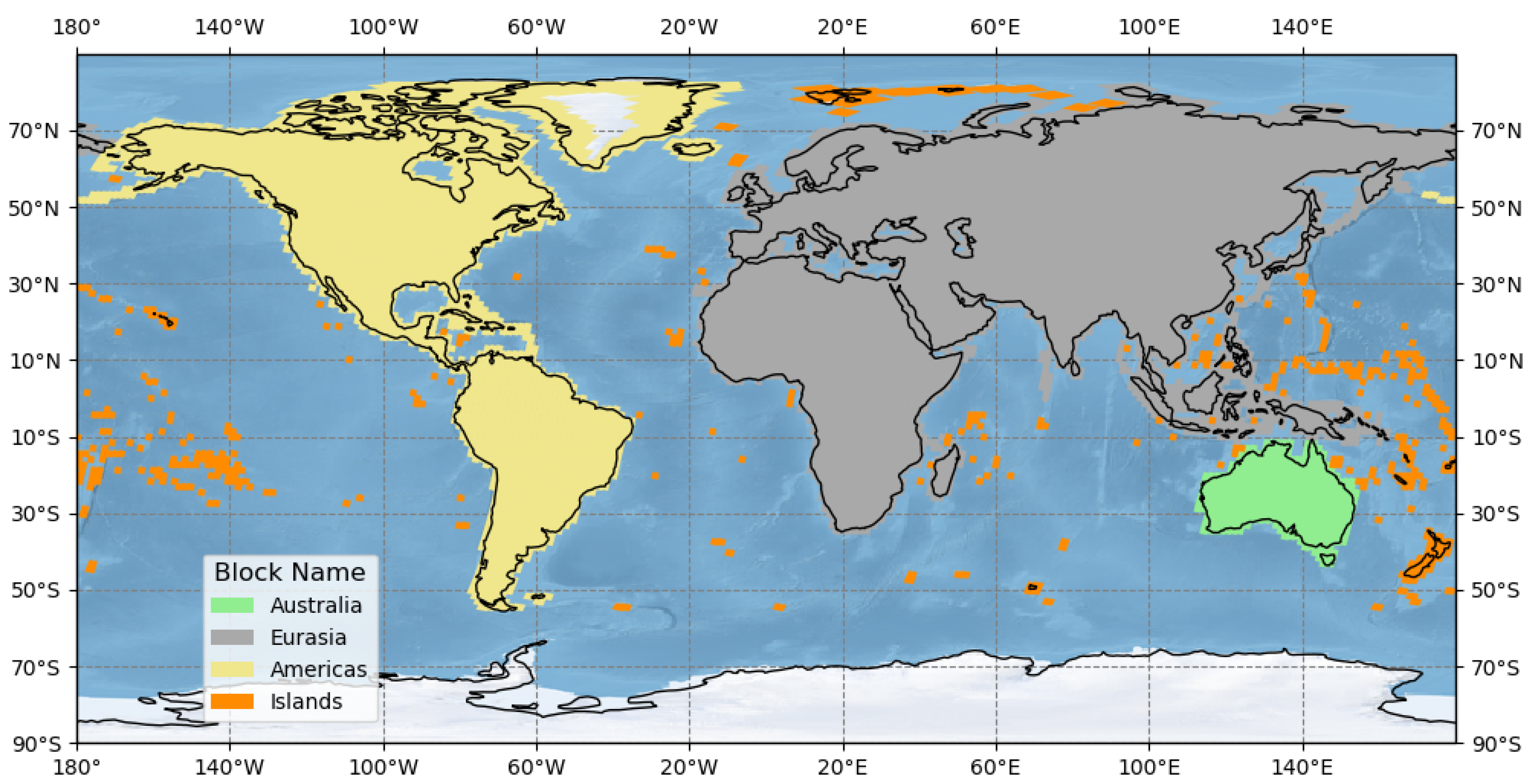
Funding

Work performed under USGS contract G15PC00012.

Acknowledgments

We would like to thank the European Space Agency for providing the GRI reference data for our analysis. We also would like to thank the USGS for supporting this research work. Any use of trade, firm, or product names is for descriptive purposes only and does not imply endorsement by the U.S. Government.

Conflicts of Interest

The authors declare no conflict of interest.

References

  1. Zhu, Z.; Wulder, M.A.; Roy, D.P.; Woodcock, C.E.; Hansen, M.C.; Radeloff, V.C.; Healey, S.P.; Schaaf, C.; Hostert, P.; Strobl, P.; et al. Benefits of the free and open Landsat data policy. Remote Sens. Environ. 2019, 224, 382–385. [Google Scholar] [CrossRef]
  2. Wulder, M.A.; Loveland, T.R.; Roy, D.P.; Crawford, C.J.; Masek, J.G.; Woodcock, C.E.; Allen, R.G.; Anderson, M.C.; Belward, A.S.; Cohen, W.B.; et al. Current status of Landsat program, science, and applications. Remote Sens. Environ. 2019, 225, 127–147. [Google Scholar] [CrossRef]
  3. Roy, D.; Wulder, M.; Loveland, T.; Allen, R.; Anderson, M.; Helder, D.; Irons, J.; Johnson, D.; Kennedy, R.; Scambos, T.; et al. Landsat-8: Science and product vision for terrestrial global change research. Remote Sens. Environ. 2014, 145, 154–172. [Google Scholar] [CrossRef] [Green Version]
  4. Wulder, M.A.; Masek, J.G.; Cohen, W.B.; Loveland, T.R.; Woodcock, C.E. Opening the archive: How free data has enabled the science and monitoring promise of Landsat. Remote Sens. Environ. 2012, 122, 2–10. [Google Scholar] [CrossRef]
  5. Miller, H.M.; Richardson, L.; Koontz, S.R.; Loomis, J.; Koontz, L. Users, uses, and value of Landsat satellite imagery—Results from the 2012 survey of users. US Geol. Surv.-Open-File Rep. 2013, 1269, 51. [Google Scholar]
  6. Storey, J.; Roy, D.P.; Masek, J.; Gascon, F.; Dwyer, J.; Choate, M. A note on the temporary misregistration of Landsat-8 Operational Land Imager (OLI) and Sentinel-2 Multi Spectral Instrument (MSI) imagery. Remote Sens. Environ. 2016, 186, 121–122. [Google Scholar] [CrossRef] [Green Version]
  7. Trémas, T.L.; Déchoz, C.; Lacherade, S.; Nosavan, J.; Petrucci, B. Sentinel-2: Presentation of the CAL/VAL commissioning phase. Int. Soc. Opt. Photonics 2015, 9643, 964309. [Google Scholar]
  8. Storey, J.; Choate, M.; Lee, K. Landsat 8 Operational Land Imager On-Orbit Geometric Calibration and Performance. Remote Sens. 2014, 6, 11127–11152. [Google Scholar] [CrossRef] [Green Version]
  9. Gutman, G.; Huang, C.; Chander, G.; Noojipady, P.; Masek, J.G. Assessment of the NASA—USGS Global Land Survey (GLS) datasets. Remote Sens. Environ. 2013, 134, 249–265. [Google Scholar] [CrossRef]
  10. Dechoz, C.; Poulain, V.; Massera, S.; Languille, F.; Greslou, D.; de Lussy, F.; Gaudel, A.; L’Helguen, C.; Picard, C.; Trémas, T. Sentinel 2 global reference image. Image and Signal Processing for Remote Sensing XXI. Int. Soc. Opt. Photonics 2015, 9643, 96430A. [Google Scholar]
  11. Storey, J.C.; Rengarajan, R.; Choate, M.J. Bundle Adjustment Using Space-Based Triangulation Method for Improving the Landsat Global Ground Reference. Remote Sens. 2019, 11, 1640. [Google Scholar]
  12. Smith, C.M.; Pagnutti, M.; Holekamp, K.; Zanoni, V.; Fendley, D. Geopositional Accuracy Assessment of EarthSat Geocover Landsat Orthorectified Imagery. 2004. Available online: https://ntrs.nasa.gov/citations/20050160940 (accessed on 22 September 2020).
  13. Dykstra, J.D.; Storey, J.C. Landsat-7 definitive ephemeris-an independent verification of GeoCover-Ortho 1990 positional accuracy. In Proceedings of the ASPRS 2004 Annual Conference Proceedings, Unpaginated CD_ROM, Denver, CO, USA, 23–28 May 2004. [Google Scholar]
  14. Tucker, C.J.; Grant, D.M.; Dykstra, J.D. NASA’s global orthorectified Landsat data set. Photogramm. Eng. Remote Sens. 2004, 70, 313–322. [Google Scholar] [CrossRef] [Green Version]
  15. Rengarajan, R.; Sampath, A.; Storey, J.; Choate, M. Validation of geometric accuracy of global land survey (GLS) 2000 data. Photogramm. Eng. Remote Sens. 2015, 81, 131–141. [Google Scholar] [CrossRef]
  16. Rengarajan, R.; Choate, M.; Storey, J. Extraction of GCP Chips From GeoCover Using Modified Moravec Interest Operator (MMIO) Algorithm; Technical Report; Department of the Interior, U.S. Geological Survey, EROS: Sioux Falls, SD, USA, 2006. Available online: https://landsat.usgs.gov/sites/default/files/documents/MMIO_GeoCover_Control_White_Paper.pdf (accessed on 22 September 2020).
  17. Gaudel, A.; Languille, F.; Delvit, J.; Michel, J.; Cournet, M.; Poulain, V.; Youssefi, D. Sentinel-2: Global Reference Image Validation and Application To Multitemporal Performances and High Latitude Digital Surface Model. Int. Arch. Photogramm. Remote Sens. Spat. Inf. Sci. 2017, 42. [Google Scholar] [CrossRef] [Green Version]
  18. Ravanbakhsh, M.; Wang, L.W.; Fraser, C.; Lewis, A. Generation of the Australian geographic reference image through long-strip ALOS PRISM orientation. ISPRS Int. Arch. Photogramm. Remote Sens. Spat. Inf. Sci. 2012, XXXIX-B1, 225–229. [Google Scholar] [CrossRef] [Green Version]
  19. USGS. Landsat 8 (L8) Calibration and Validation (Cal/val) Algorithm Description Document (ADD); Technical Report; Department of the Interior, U.S. Geological Survey, EROS: Sioux Falls, SD, USA, 2015. Available online: https://prd-wret.s3.us-west-2.amazonaws.com/assets/palladium/production/atoms/files/LSDS-1747_Landsat8-9_CalVal_ADD-v3.pdf (accessed on 22 September 2020).
  20. Clerc, S. Sentinel-2 L1C Data Quality Report; Technical Report. ESA: Paris, France, 2020. Available online: https://sentinel.esa.int/web/sentinel/user-guides/sentinel-2-msi/document-library/-/asset_publisher/Wk0TKajiISaR/content/sentinel-2-data-quality-report-issue-03-may-2016- (accessed on 22 September 2020).
  21. Mukherjee, S.; Joshi, P.; Mukherjee, S.; Ghosh, A.; Garg, R.; Mukhopadhyay, A. Evaluation of vertical accuracy of open source Digital Elevation Model (DEM). Int. J. Appl. Earth Obs. Geoinf. 2013, 21, 205–217. [Google Scholar] [CrossRef]
  22. Rodriguez, E.; Morris, C.S.; Belz, J.E. A global assessment of the SRTM performance. Photogramm. Eng. Remote Sens. 2006, 72, 249–260. [Google Scholar] [CrossRef] [Green Version]
  23. Lee, D.S.; Storey, J.C.; Choate, M.J.; Hayes, R.W. Four years of Landsat-7 on-orbit geometric calibration and performance. IEEE Trans. Geosci. Remote Sens. 2004, 42, 2786–2795. [Google Scholar] [CrossRef]
  24. USGS. Landsat Collection 1 Level 1 Product Definition; Technical Report; Department of the Interior, U.S. Geological Survey, EROS: Sioux Falls, SD, USA, 2019. Available online: https://prd-wret.s3.us-west-2.amazonaws.com/assets/palladium/production/atoms/files/LSDS-1656_%20Landsat_Collection1_L1_Product_Definition-v2.pdf (accessed on 22 September 2020).
  25. USGS. Landsat Geometry. 2020. Available online: https://landsat.usgs.gov/gcp (accessed on 22 September 2020).
Figure 1. Map of triangulation blocks used in the bundle adjustment process.
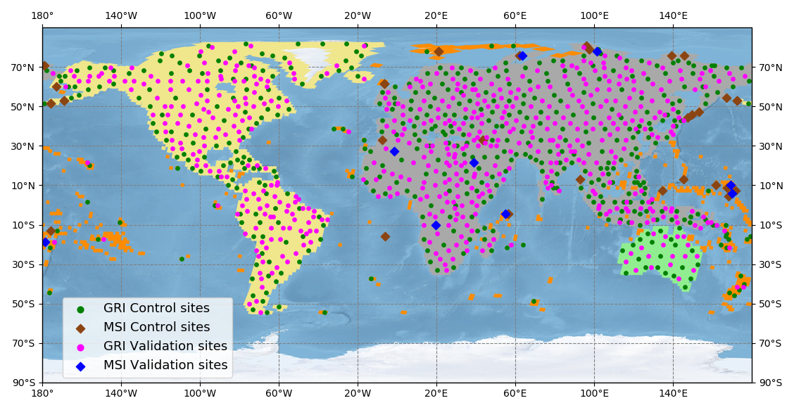
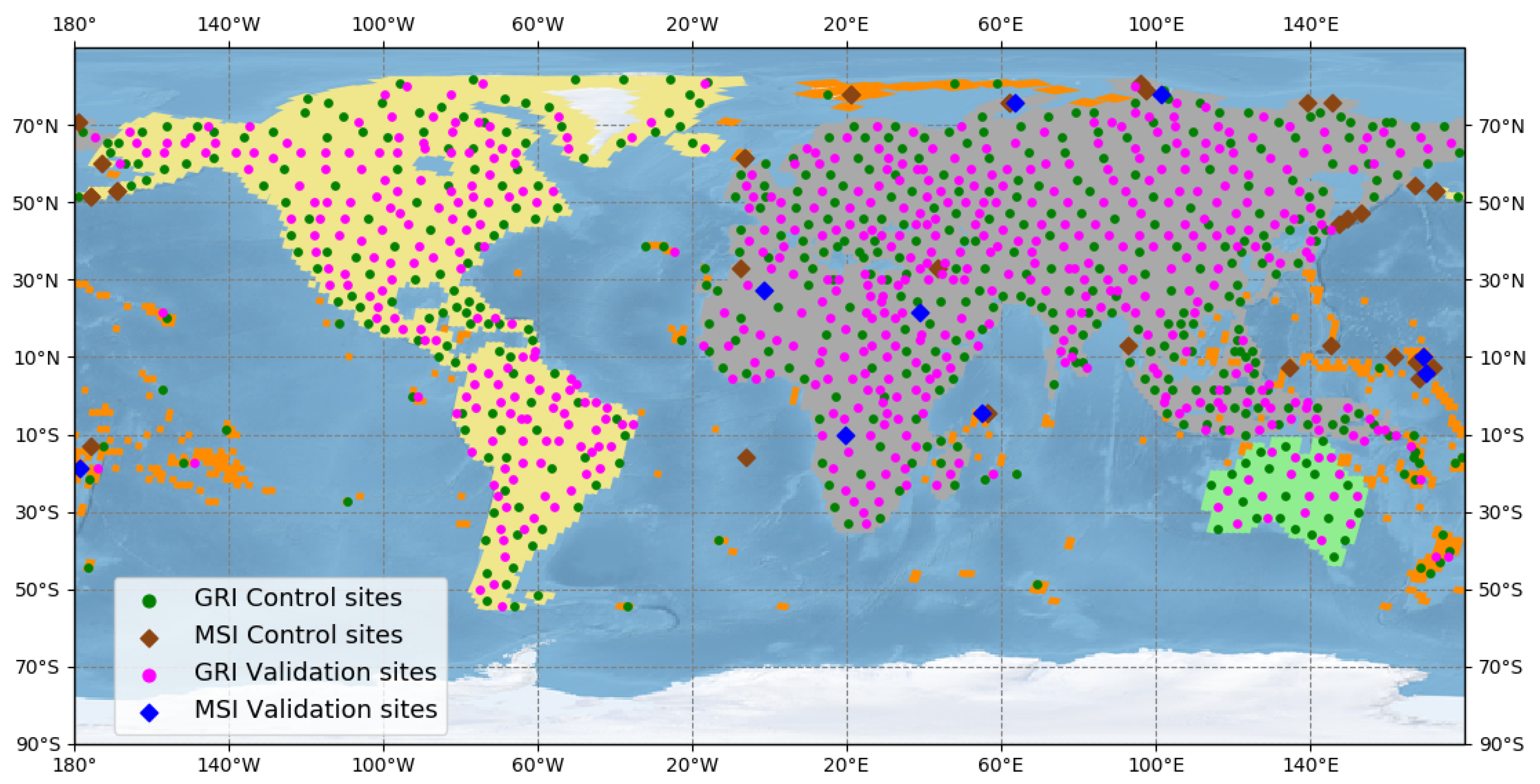
Remotesensing 12 03132 g001
Figure 2. Control and Validation sites used in the block triangulation procedure. The green and magenta circles represent the Global Reference Image (GRI) control and validation tiles, respectively. The brown and blue diamonds represent the Multispectral Imager (MSI) control and validation tiles, respectively.
Remotesensing 12 03132 g002
Figure 3. Schematic flow of how GRI- and Landsat-8-derived Ground Control Points (GCPs) are used in the bundle adjustment techniques. The triangulation-based bundle adjustment provides correction estimates for the spacecraft information (ephemeris, velocity, attitude, attitude rate) along with position updates for the GCPs, but we are interested only in the updates to the GCP positions.
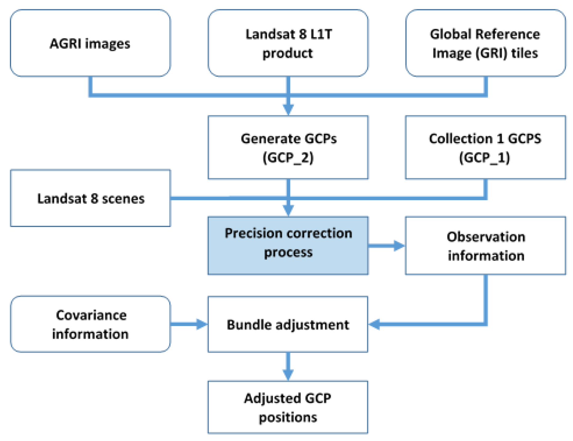
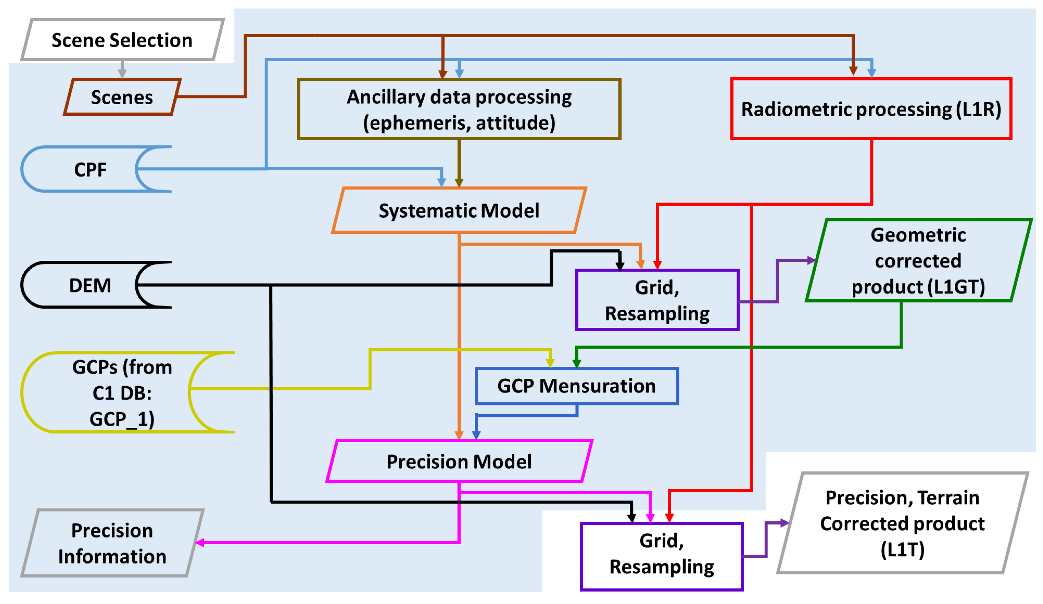
Remotesensing 12 03132 g003
Figure 4. A simplified version of the Landsat process flow for generating terrain-corrected products. The shaded (transparent blue) portion shows the algorithm used in the precision correction process. Each input, output, and process shape is color-coded, and the arrows from them are also color-coded for ease of understanding. For example, a Calibration Parameter File (CPF) stores the calibration parameters and, therefore, is shown using the corresponding flowchart shape with a blue border. The CPF is used in ancillary data processing, systematic model generation, and in the radiometric processing, and is therefore shown in blue arrows.
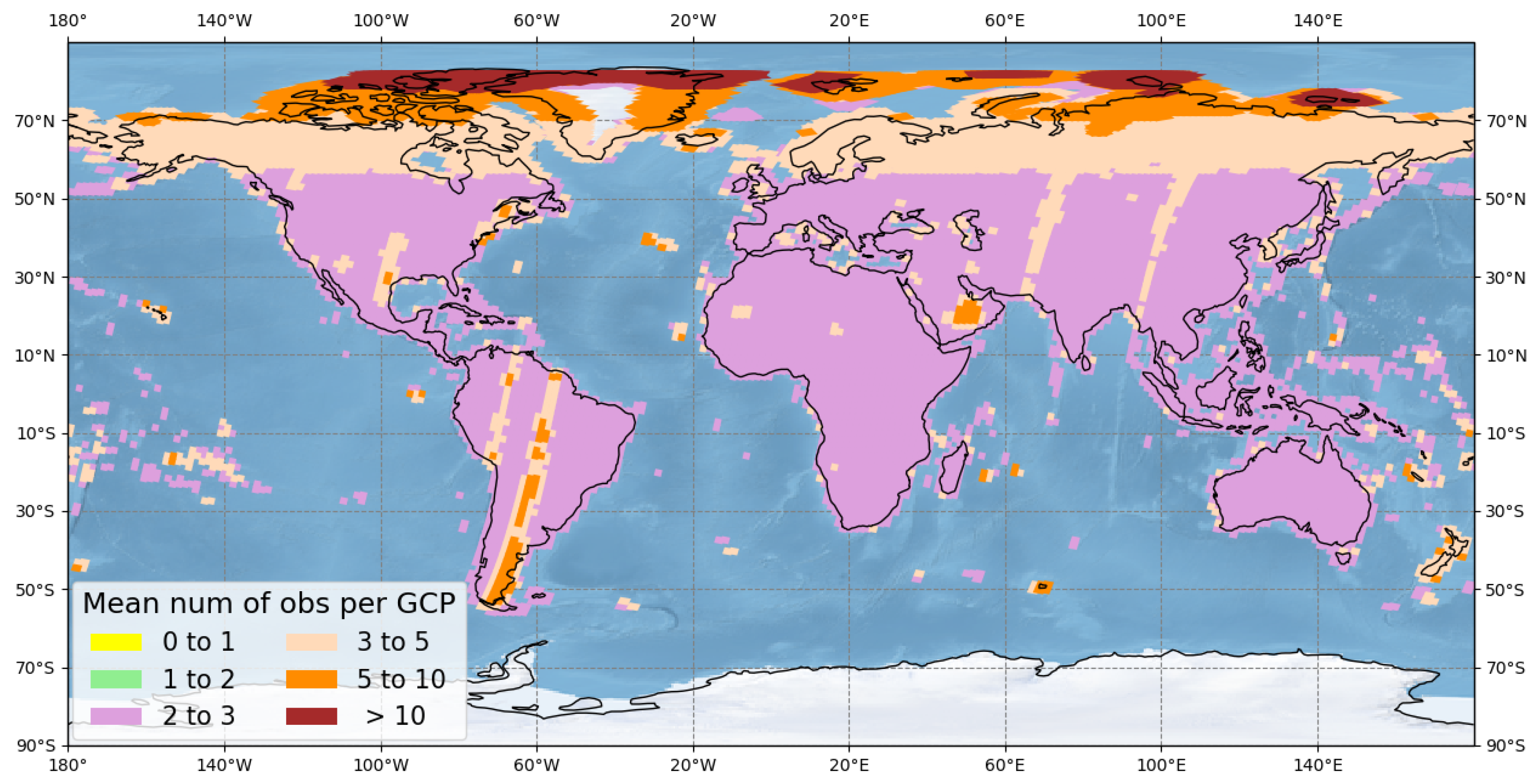
Remotesensing 12 03132 g004
Figure 5. Average number of observations per GCP for each World Reference System (WRS)-2 path/row used in the bundle adjustment procedure. The large overlap in the northern latitudes generates a higher number of observations per GCP.
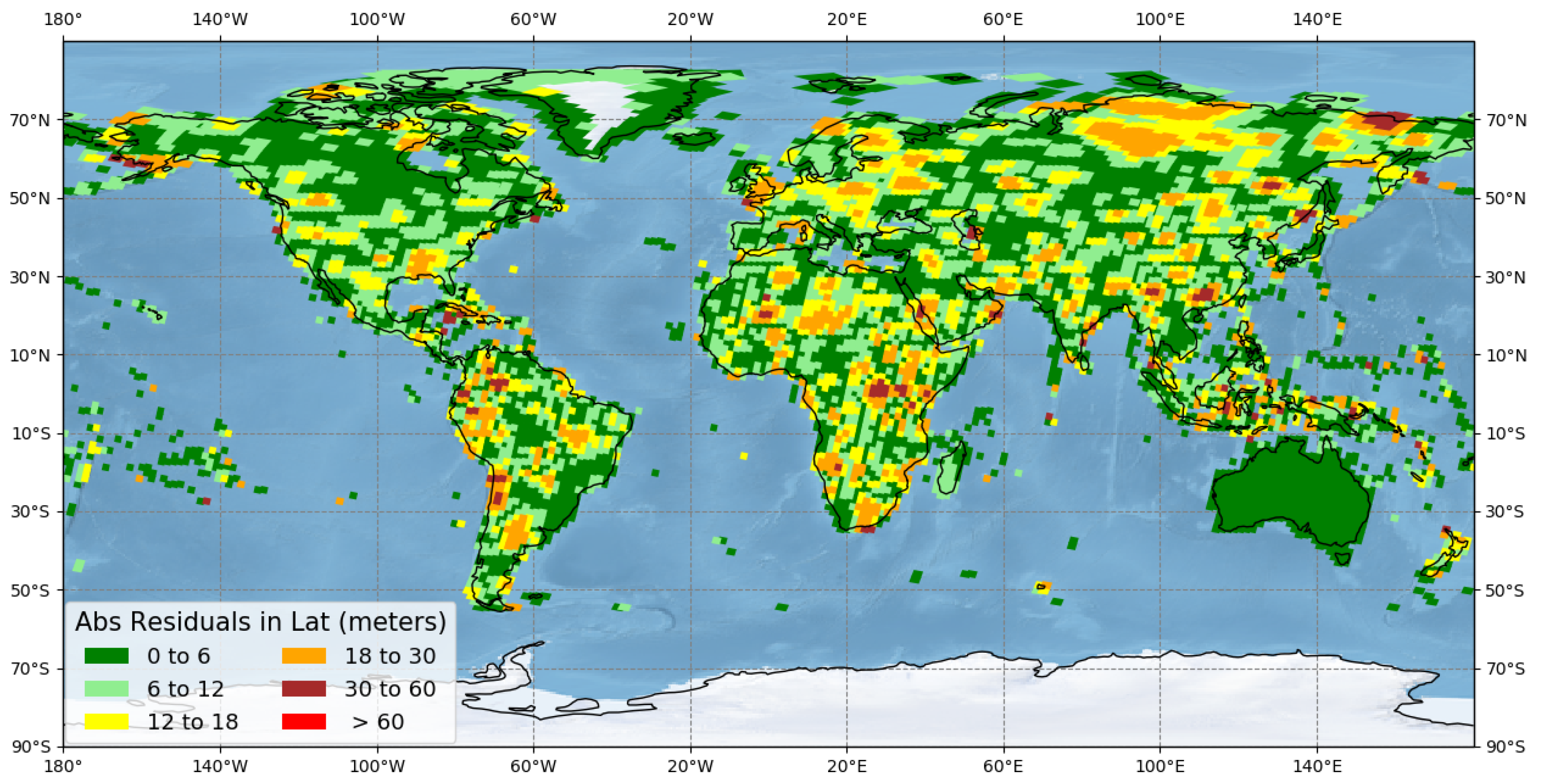
Remotesensing 12 03132 g005
Figure 6. Mean residuals of the GCPs in the latitude direction for each of the WRS-2 paths/rows, computed from the block triangulation solution.
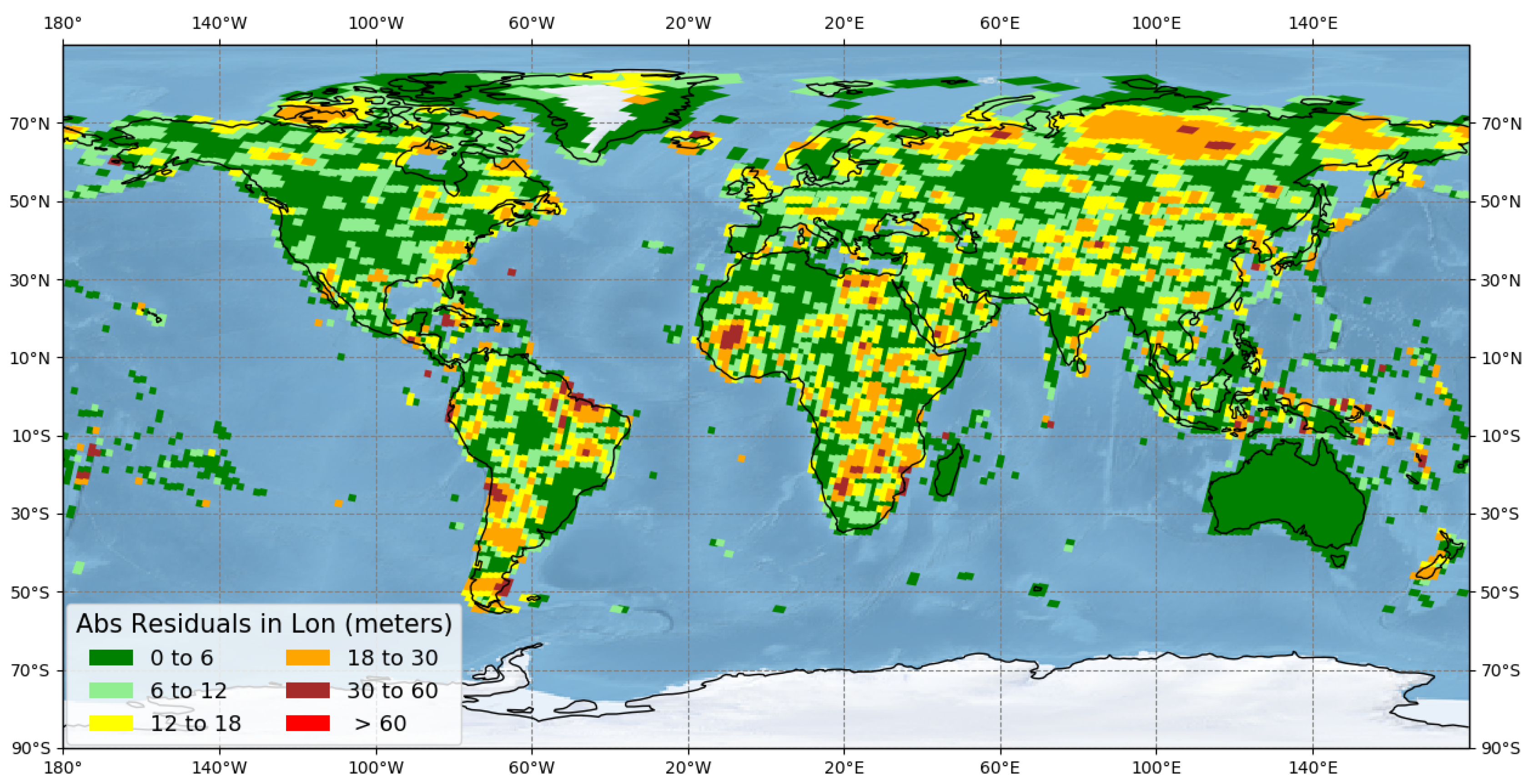
Remotesensing 12 03132 g006
Figure 7. Mean residuals of the GCPs in the longitude direction for each of the WRS-2 paths/rows, computed from the block triangulation solution.
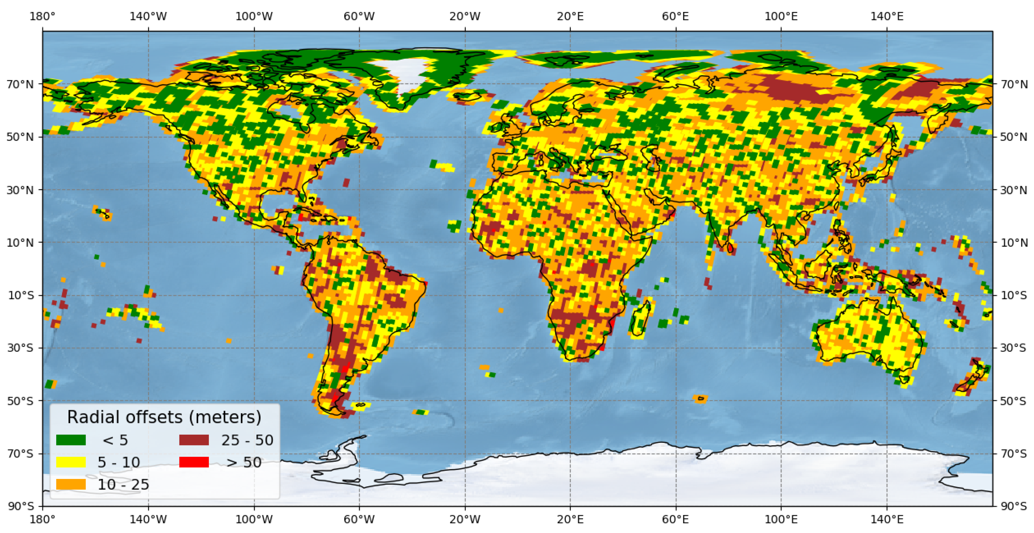
Remotesensing 12 03132 g007
Figure 8. Radial geodetic offsets of the Landsat 8 (L8) scenes processed using the Collection-1 GCPs.
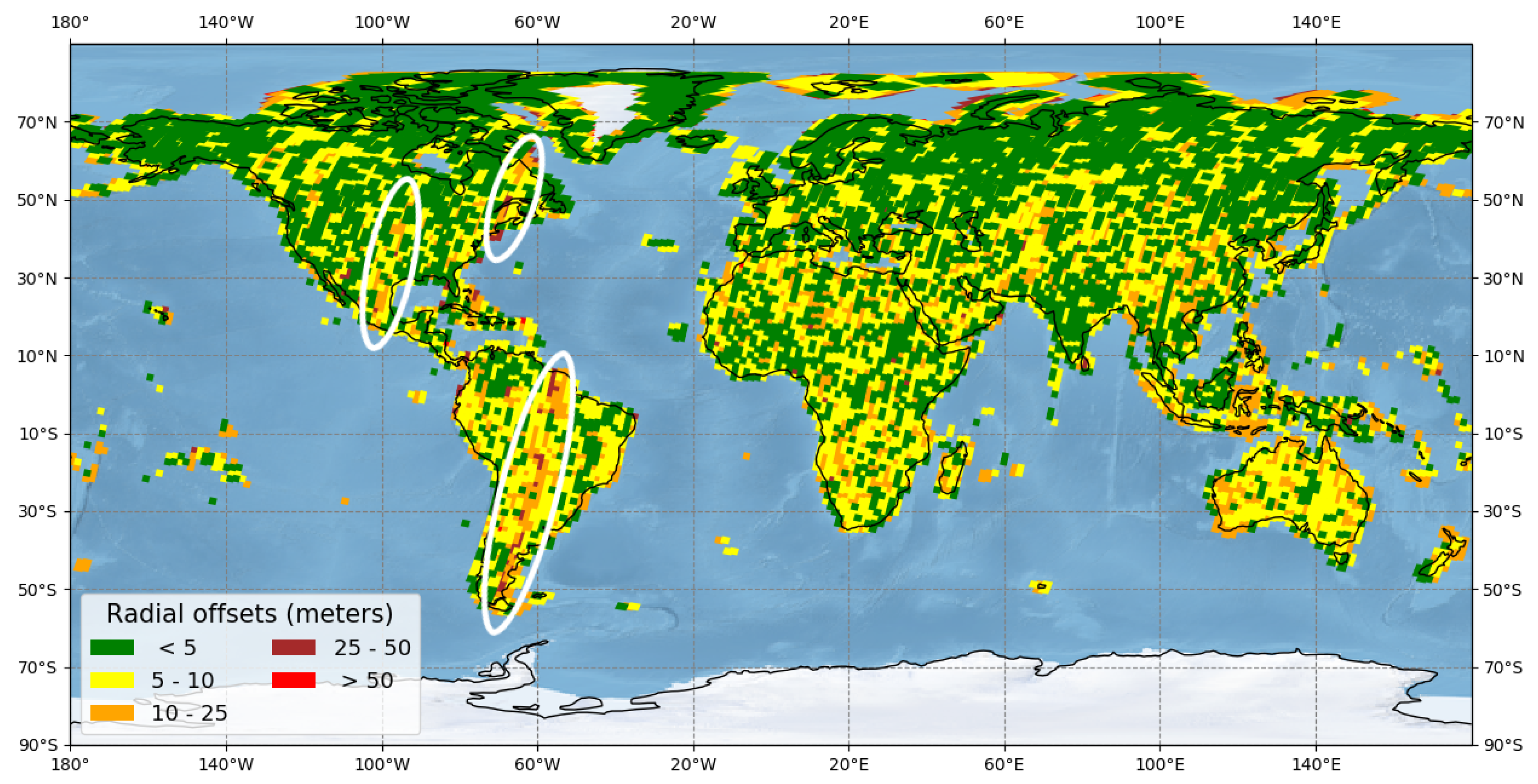
Remotesensing 12 03132 g008
Figure 9. Radial geodetic offsets of the L8 scenes processed using the updated GCPs.
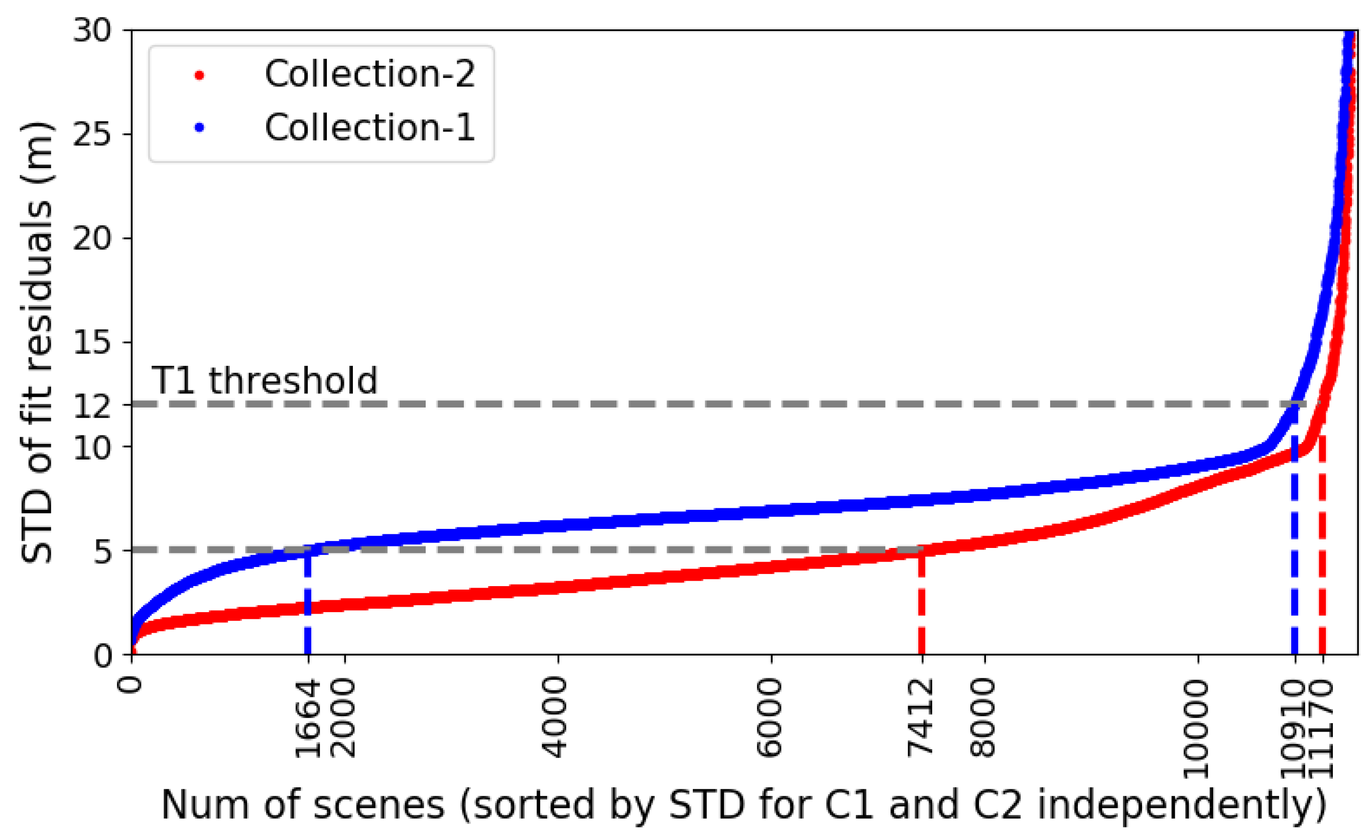
Remotesensing 12 03132 g009
Figure 10. Comparison of the STD from the precision model fit residuals between Collection-1 and Collection-2 processing of the test scenes. The red and blue lines indicate the STD for the Collection-2 and Collection-1 products, respectively. The Collection-2 products show significantly lower STDs than Collection-1 products.
Remotesensing 12 03132 g010
Table 1. Number of Global Reference Image (GRI) control and validation tiles used in the triangulation block.
Block NameNumber of UniqueUnique GRI TilesGRIGRIUniqueMSIMSI
GRI Images(Unique Locations)Control TilesValidation TilesMSI TilesControl TilesValidation Tiles
Australia77372116000
Americas1006310138172770
Eurasia195362627934721165
Islands15947361118144
Total3195102047454646379
Table 2. Standard deviations used to determine the weights or a priori covariance in the space-based triangulation method. Note that the AGRI and GRI GCPs were heavily weighted (small Standard Deviation (STD)) to add constraints to the bundle adjustment so that most of the adjustments are imparted to the Global Land Survey (GLS) GCPs.
ParametersStandard Deviations (to Construct Covariance)Units
GLS GCP (lat, lon, ht)(10000, 10000, 30)meters
AGRI GCP (lat, lon, ht)(5, 5, 5)meters
GRI GCP (lat, lon, ht)(5, 5, 5)meters
MSI GCP (lat, lon, ht)(10, 10, 5)meters
Image Point (x, y)(5,5)meters
Ephemeris/Position (X, Y, Z)(4, 4, 4)meters
Ephemeris rate/Velocity (X, Y, Z)(0.001, 0.001, 0.001)meters
Attitude (roll, pitch, yaw)(1 × 10 5 , 1 × 10 5 , 1 × 10 5 )radians
Attitude rate (roll, pitch, yaw)(1 × 10 8 , 1 × 10 8 , 1 × 10 8 )radians
Time constant for attitude correlation60seconds
Table 3. A sample record for the four input files used in the triangulation method. The input files contain a priori information and are linked with each other by a unique identifier. The description for the comma-separated values is provided at the top for each of the files.
Input FileSample Record
PassPassID, Path, Year, DOY, PassCenterTime, W X , W Y , W Z , W V x , W V y , W V z
fileP0982014280, 098, 2014, 280, 2026.105844, 4.0, 4.0, 4.0, 0.001, 0.001, 0.001
ImageImageID, PassID, Path, Row, Year, DOY, ImageCenterTime, TimeConst,
file W R o l l , W P i t c h , W Y a w , W R r a t e , W P r a t e , W Y r a t e
 I0982014280069, P0982014280, 098, 069, 2014, 280, 2039.397235, 60.0,
 1.0 × 10 5 , 1.0 × 10 5 , 1.0 × 10 5 , 1.0 × 10 8 , 1.0 × 10 8 , 1.0 × 10 8
ObservationObsID, G C P I D , ImageID, Year, DOY, ObsTime,
fileX, Y, Z, V X , V Y , V Z , L O S x , L O S y , W x , W y ,
 dx/dSample, dx/dLine, dy/dSample, dy/dLine
 O098201428006900539, G098069GLS0347, I0982014280069, 2014, 280, 2030.4219,
 −5,511,185.7, 4,178,211.06, −1,538,758.9, 1941.53642, −94.802, −7244.9214, −0.010875994, −0.054445814, 5.0, 5.0,
 −2.0400 × 10 7 , −1.3980 × 10 6 , −1.3970 × 10 6 , 2.0500 × 10 7
Ground G C P I D , lat, lon, ht, W l a t , W l o n , W h
fileG098069GLS0347, -12.607373064, 143.194174804, 339.089, 10000.0, 10000.0, 30.0
Table 4. Number of observations, passes, images, and GCPs used for each triangulation block in the space-based bundle adjustment procedure.
Block NameNumber of ObservationsNumber of ImagesNumber of PassesNumber of GCPs
GLSGRIMSIAGRI
Australia581,706405274286,1158462010,897
Americas5,029,280363618451,595,42098,3926560
Eurasia7,938,901567329933,228,007175,281683347
Islands236,17599384454,573,21,77335360
Total13,786,06210,70759565,164,115303,90811,02510,944
Table 5. Number of iterations and the initial and final root mean square (RMS) error of the observations in the bundle adjustment for each block. The Australia block showed smaller RMS error before bundle adjustment, as the GCPs were adjusted using the AGRI reference dataset.
Block NameNumber of IterationsRMS Error (Micro-Radians)
Before Bundle AdjustmentAfter Bundle Adjustment
Australia29.33 × 10 6 1.97 × 10 6
Americas21.80 × 10 5 2.79 × 10 6
Eurasia21.89 × 10 5 2.63 × 10 6
Islands21.90 × 10 5 3.63 × 10 6
Table 6. Validation of the GCP updates using the geodetic accuracy validation procedure for the Australia block.
TypeNumber ofMeanMeanSTDSTDConsistencyConsistency
ScenesXT (m)AT (m)XT (m)AT (m)XT (m)AT (m)
Collection-1Control224.31−4.094.135.131.582.08
Updated GCPsControl223.87−5.184.114.611.091.83
Collection-1Validation173.95−4.204.933.901.502.04
Updated GCPsValidation173.65−4.634.834.411.271.78
Updated GCPs (all)Validation173.70−4.694.794.321.231.69
Table 7. Validation of the GCP updates using the geodetic accuracy validation procedure for all the blocks. One scene per land path/row was processed using GCPs before and after bundle adjustment for each block.
BlockTypeNumber ofMeanMeanSTDSTDConsistencyConsistency
ScenesXT (m)AT (m)XT (m)AT (m)XT (m)AT (m)
AustraliaCollection-14044.61−4.204.784.932.232.70
Updated GCPs4044.10−4.804.494.761.962.49
AmericasCollection-131560.720.9413.2510.676.706.22
Updated GCPs31560.730.817.706.432.973.20
EurasiaCollection-15421−1.030.6213.3511.817.306.93
Updated GCPs5421−1.29−1.856.035.622.923.27
IslandsCollection-1387−1.14−0.0912.9011.236.837.57
Updated GCPs387−1.69−1.307.147.894.414.65
Table 8. Validation results for the Australia block using Image-to-Image characterization between the Sentinel-2 GRI tiles and Landsat 8 Level-1 terrain-corrected (L1T) products that were processed before (GLS) and after (Adjusted GCPs) bundle adjustment.
TypeNumber of TilesGLSAdjusted GCPs
RMSErCE90RMSErCE90
Control444.787.253.465.25
Validation334.637.023.745.68
All774.717.153.585.44
Table 9. Validation of the GCP updates using the geodetic accuracy validation procedure for the Americas block.
TypeNumber ofMeanMeanSTDSTDConsistencyConsistency
ScenesXT (m)AT (m)XT (m)AT (m)XT (m)AT (m)
Collection-1Control1611.70.4414.6410.917.476.48
Updated GCPsControl1611.260.978.297.212.162.57
Collection-1Validation1913.041.1716.612.717.366.54
Updated GCPsValidation1912.030.57.445.572.112.50
Updated GCPs (all)Validation1912.040.507.425.52.002.42
Table 10. Validation results for the Americas block using Image-to-Image characterization between the Sentinel-2 GRI tiles and Landsat 8 L1T products that were processed before (GLS) and after (Adjusted GCPs) bundle adjustment.
TypeNumber of TilesGLSAdjusted GCPs
RMSErCE90RMSErCE90
Control47214.8222.485.047.65
Validation53416.3324.774.596.96
Control + Validation100615.6423.734.817.29
MSI Validation818.0527.398.5112.92
Table 11. Validation of the GCP updates using the geodetic accuracy validation procedure for the Eurasia block.
TypeNumber ofMeanMeanSTDSTDConsistencyConsistency
ScenesXT (m)AT (m)XT (m)AT (m)XT (m)AT (m)
Collection-1Control309−1.05−0.1011.2911.147.637.43
Updated GCPsControl309−1.79−2.425.535.132.222.78
Collection-1Validation375−0.010.3513.9814.027.827.11
Updated GCPsValidation376−1.03−1.795.224.942.012.42
Updated GCPs (all)Validation380−1.09−1.675.134.921.902.33
Table 12. Validation results for the Eurasia block using Image-to-Image characterization between the Sentinel-2 GRI tiles and Landsat 8 L1T products that were processed before (GLS) and after (Adjusted GCPs) bundle adjustment.
TypeNumber of TilesGLSAdjusted GCPs
RMSErCE90RMSErCE90
Control83816.4124.904.256.45
Validation111518.4227.964.496.81
Control + Validation195317.5926.694.396.66
MSI Validation5319.0028.837.9712.09
Table 13. Validation of the GCP updates using the geodetic accuracy validation procedure for the Islands block.
TypeNumber ofMeanMeanSTDSTDConsistencyConsistency
ScenesXT (m)AT (m)XT (m)AT (m)XT (m)AT (m)
Collection-1Control82−4.65−1.8216.3011.806.277.03
Updated GCPsControl821.21−5.134.875.762.773.49
Collection-1Validation301.57−8.2812.1111.525.967.23
Updated GCPsValidation301.83−3.315.726.262.843.61
Updated GCPs (all)Validation301.94−3.355.546.162.693.50
Table 14. Validation results for the Islands block using Image-to-Image characterization between the Sentinel-2 GRI tiles and Landsat 8 L1T products that were processed before (GLS) and after (Adjusted GCPs) bundle adjustment.
TypeNumber of TilesGLSAdjusted GCPs
RMSErCE90RMSErCE90
Control11519.0228.865.318.06
Validation4417.4226.437.7311.73
Control + Validation15918.5928.216.089.22
MSI Validation4121.1432.087.2711.03
Table 15. Comparison of the product type expected in Collection-2 with the corresponding product types in Collection-1. One scene for each land path/row was processed using Collection-1 GCPs (Collection-1) and bundle-adjusted GCPs (Collection-2) using the same processing system. More L1TP (T1) products are expected to be generated in Collection-2 than in Collection-1.
Collection-2
L1TP-T1L1TP-T2L1GTTotal
Collection-1L1TP-T110,87436410,914
L1TP-T229625516567
L1GT19241289522
Total11,36233230912,003

