Estimation of Snow Depth in the Hindu Kush Himalayas of Afghanistan during Peak Winter and Early Melt Season


1
Department of Environment Bio-Production Engineering, Tokyo University of Agriculture, Tokyo 156-8502, Japan
2
Faculty of Engineering Geology and Mines, Jowzjan University, Jowzjan 1901, Afghanistan
3
National Centre for Geodesy, Indian Institute of Technology Kanpur, Kanpur 208016, India
*
Author to whom correspondence should be addressed.
Remote Sens. 2020, 12(17), 2788; https://0-doi-org.brum.beds.ac.uk/10.3390/rs12172788
Submission received: 9 July 2020
/
Revised: 21 August 2020
/
Accepted: 24 August 2020
/
Published: 27 August 2020
(This article belongs to the Special Issue Recent Advances in Cryospheric Sciences)
Abstract
:The Pamir ranges of the Hindu Kush regions in Afghanistan play a substantial role in regulating the water resources for the Middle Eastern countries. Particularly, the snowmelt runoff in the Khanabad watershed is one of the critical drivers for the Amu River, since it is a primary source of available water in several Middle Eastern countries in the off monsoon season. The purpose of this study is to devise strategies based on active microwave remote sensing for the monitoring of snow depth during the winter and the melt season. For the estimation of snow depth, we utilized a multi-temporal C-band (5.405 GHz) Sentinel-1 dual polarimetric synthetic aperture radar (SAR) with a differential interferometric SAR (DInSAR)-based framework. In the proposed approach, the estimated snowpack displacements in the vertical transmit-vertical receive (VV) and vertical transmit-horizonal receive (VH) channels were improved by incorporating modeled information of snow permittivity, and the scale was enhanced by utilizing snow depth information from the available ground stations. Two seasonal datasets were considered for the experiments corresponding to peak winter season (February 2019) and early melt season (March 2019). The results were validated with the available nearest field measurements. A good correlation determined by the coefficient of determination of 0.82 and 0.57, with root mean square errors of 2.33 and 1.44 m, for the peak winter and the early melt season, respectively, was observed between the snow depth estimates and the field measurements. Further, the snow depth estimates from the proposed approach were observed to be significantly better than the DInSAR displacements based on the correlation with respect to the field measurements.
1. Introduction
Afghanistan is a country that is extensively affected by dry weather, and most of the land in this country is arid. The population of this country is predominantly dependent upon seasonal and glacial snowmelt water for irrigation, hydropower, and domestic purposes [1]. The Hindu Kush Himalayan regions exhibit a substantial amount of seasonal snow cover during the winters in the Asian subcontinent. During the summer, snowmelt leads to a majority of the available water resource in the Asian subcontinent. The estimated annual runoff from glaciers and the snowmelt accounts for ca. 30–50% of the river water [2]. Therefore, glaciers and seasonal snow are the major resources for regional water availability and the hydrological system. The global energy balance, natural disasters, such as floods, riverbank erosion, and avalanches are also largely affected by the seasonal snow volume [3].
Based on the World Bank report in 2015 on the assessment of the role of glaciers in streamflow from the Pamir and Tien Shan mountains, the total amount of snowmelt runoff in the Amu Darya has been estimated to be 79 km3. Out of this, 34 km3 snowmelt water is contributed from the Panj River of Afghanistan [4]. Although the primary source of the Amu Darya water is usually from precipitation, a substantial annual contribution is from glacier and snowmelt, which originates from high mountains of Hindu Kush Pamir [4]. The Amu Darya, where Darya refers to a ‘River,’ is driven by water contributed from the melting of high-mountain snow and glaciers during spring and the summer seasons and by rain precipitation during the monsoon. The mean long-term runoff of Amu Darya is 73.5 km3. The primary runoff volume (up to 85%) is formed by the Vakhsh and Pyandzh tributaries of the Amu Darya [4,5]. About 15% of the total runoff is contributed by the Surkhandarya, Kafirnigan, and Kunduz tributaries. The annual runoff variability in the long-term regime is low (the coefficient of variation is 0.15). However, the irregularity of the interannual distribution is substantially high. About 77–80% of the annual runoff occurs between April to September, and only 10–13% between December to February, which is usually advantageous for irrigation purposes [6].
Historically, field measurements of snow depth and snow density have been carried out using a variety of mechanical and electronic equipment [7]. These types of equipment can only be used for precise point measurements of snow depth and snow density. Issues with point measurements include the lack of spatial variability in the snow-covered mountainous regions since it is challenging to move around with such equipment. Furthermore, field campaigns for such measurements are restricted by the weather conditions, regional aspects such as militant insurgency in Afghanistan, and poor logistics. Therefore, remote sensing offers a valuable tool for obtaining spatiotemporal information on the snowpack geophysical parameters. These parameters are vital inputs for establishing information on the snow hydrological potential [8]. The hydrological potential of snow is conventionally determined by the snow water equivalent (SWE). The SWE indicates the total volume of water represented by the snowpack and is mathematically derived as the product of the snow depth and snow density [9].
Microwave remote sensing holds numerous advantages over optical remote sensing for the studies on snow hydrology, particularly due to the higher penetrability of the microwave signal [8]. In the literature, some models quantitatively determine the snow density using multispectral data [10,11]. However, these inferences are only limited to the snowpack surface. Passive microwave (PM) observations have been widely used to derive inferences on snow depth and SWE in the literature [12]. Generally, snow depth and the snow density which are used for the determination of SWE are not highly correlated. Therefore, during field surveys for the quantitative determination of these two parameters, they must be considered independent [13]. The deeper the snowpack, the higher the attenuation of the passive microwave signal. This inverse relationship between snow depth and temperature brightness is the basis of SWE retrieval from PM measurements [14]. Airborne Lidar measurements provide relatively accurate estimates of snow depth. However, Lidar data is usually affected by the weather conditions and is typically applied at a regional scale [15]. Polarimetric and interferometric synthetic aperture radar (SAR) techniques have been effectively used for the modeling of snow depth and SWE [16,17]. However, such techniques are affected by the presence of moisture in the snowpack. Fundamentally, snow dielectric properties are modified by the presence of liquid water content (LWC) in the snowpack. The presence of LWC in snow increases its effective dielectric constant and reduces the capacity of snow penetration of the radar signal [16].
SAR interferometry has been widely used in the literature [17] for the investigation of surface subsidence and or upliftment. Subsequently, in the literature, Differential Interferometric SAR (DInSAR) data has been effectively utilized for the modeling of snow depth and SWE [18,19]. Guneriussen et al. [20,21] proposed initially the snow phase model for dry snow to determine the changes in the snow water equivalent based on the DInSAR data. Several factors compromise the displacement retrieved from interferometric SAR (InSAR) processing inclusive of temporal decorrelation, geometric distortions, phase wrapping ambiguities, etc. However, it is still widely used for snow depth estimation at regional scales [16,19]. By combining remote sensing data and field measurements of snow depth, higher accuracy of snow depth estimates can be achieved [22,23].
The relatively higher revisit time of the Sentinel-1 satellites enables the formulation of successive interferometric pairs that are crucial for snowpack monitoring [23,24]. In the literature, methods have been developed to account for some of the issues related to DInSAR based snow depth estimation, including those for biases occurring because of the volume scattering of the snowpack and the phase unwrapping errors [23]. The modifications in the conventional method are particularly used to accommodate the underestimation of snow depth using DInSAR. Varade et al. [23] improved the snow depth estimates determined from the dual polarimetric DInSAR displacements in VV and VH channels. They incorporated two different bias corrections, scale adjustment, and utilized a weighted sum strategy for integrating the corrected displacements in the VV and the VH channels.
In this study, we define a framework for the estimation of snow depth inspired by Varade et al. [23]. In the proposed framework, the implications of the snow volume scattering are incorporated in the DInSAR based displacement rather than the snow phase, as in Varade et al. [23]. We avoid the phase bias correction as the test area in our study is substantially larger, which may result in an extremely higher computational complexity. Additionally, rather than relying on the field measurements for scale adjustment, we utilize information from the ground stations available in the study area. Another aspect of this study is to investigate the capability of Sentinel-1 C-band DInSAR data for the potential determination of snow depth in the melt season. Finally, we would also like to highlight the significance of this study from the perspective of snow hydrological monitoring in Afghanistan.
2. Study Area and Materials Used
The primary water resource of Amu Darya (River) is the seasonal snow in the Hindu Kush mountains of Afghanistan. The Amu Darya originates from the Pamir Hindu Kush mountains, and it has the largest mean long-term runoff in the Aral Sea [4]. Moreover, almost all rivers of northern Afghanistan are driven from this mountain range and flow towards north and northwest. Based on the hydrograph and hydrological aspects, almost all the river basins in this area are divided into sub-basins. In the North Afghanistan Panj-Amu Darya basin includes main tributary rivers Kunduz, Kokcha, and Khanabad watershed also joins with the Kunduz river [25].
2.1. Study Area and Test Data
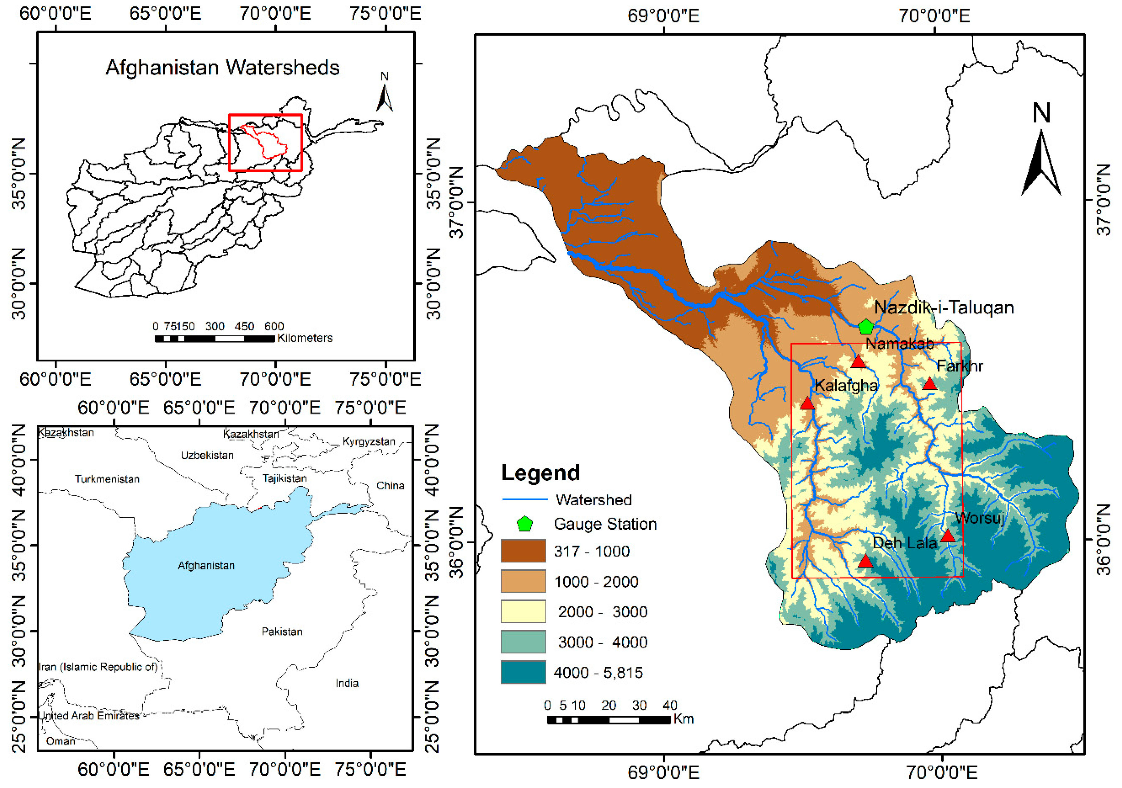
Typically, the high and semi-elevated areas of the Hindu Kush mountains in north Afghanistan experience heavy snowfall. Generally, Autumn and Winter precipitation (October to March) accumulates in the form of snow, especially in the higher elevation regions [5]. The accumulated snow begins to melt at increased rates from the late spring season. The snowmelt rate increases further afterward from June to August, subsequently leading to summer floods and riverbank erosion downstream [26]. The investigation area in this study is located in the Takhar province with the geographical coordinates of 37°11′58.16″ N and 70°31′28.91″ E, and an average altitude of 3224 m. Typically, the Takhar province experiences relatively high seasonal snow accumulation. This region shares its borders with the northeastern Panjshir, Baghlan, and Kunduz provinces in northern Afghanistan. The area investigated in this study covers the mountain ranges of the Hindu Kush in the southern part of the basin in the Khanabad watershed, shown in Figure 1. The Khanabad watershed covers a vast agricultural land and flood plains comprising highly fertile medium-grained soil that has a substantial impact on the agro-economical aspects of this region. The total area of the Khanabad watershed is about 11,988 km2. Table 1 shows the Sentinel-1 datasets used for the modeling of snow depth in this study, where the displacements are computed using the reference snow cover scene and the snow-free scene (i.e., 20 September 2018) corresponding to which the temporal baseline is defined. For the modeling of snow permittivity, the reference and the nearest scenes are used. The reference scenes were selected to have the minimum difference in duration with respect to the field measurements. The nearest scene is the closest available Sentinel-1 scene corresponding to the reference scene and sensed before it. For the determination of the snow cover area (SCA) for both datasets (peak winter, i.e., February 2019, and early melt season, i.e., March 2019) the Landsat-8 Operational Land Imager (OLI) multispectral data were used.
2.2. Field Data Collection
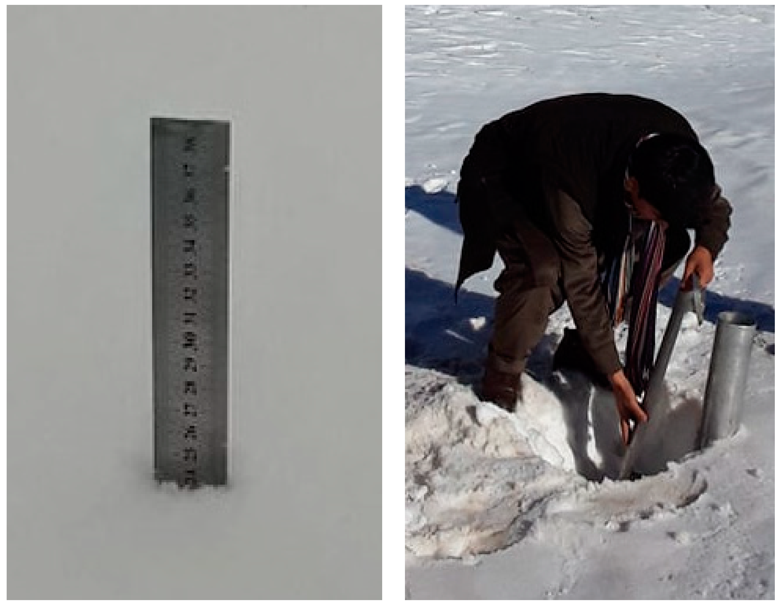
Generally, the snow depth in the Khanabad watershed is in the order of a few meters in the peak winter to the melt season. In this study, for the validation, we utilized the snow depth measurements obtained from 40 points during the field campaigns conducted in February and March 2019, by a survey team from General Affairs of Snow and Glacier Analysis, Department of Surface Water, General Directorate of Water Resources, National Water Affairs Regulation Authority (GMSGA), Afghanistan. These measurements were collected at two locations near Worsaj and Kalafgan (Figure 1), at an average elevation of 2666 m and 2243 m, respectively. Figure 2 shows the field photographs corresponding to one of the campaigns for the snow depth measurement. The layout of the observations was evenly distributed as much as possible, with the typical difference between each point observation taken at 2 m extending in four directions, i.e., North-East-South-West. The snow depth measurements were collected from rulers and snow tubes. The data acquisition frequency was once per day, and the data acquisition time was between 13:00–15:00 h. The field measurements of 15 February and 23 March, 2019, were used for this study for validation of the proposed method. Amongst these measurements, the maximum and the minimum snow depth was observed to be 75 cm and 60 cm, respectively.
3. Methodology
3.1. Proposed Framework
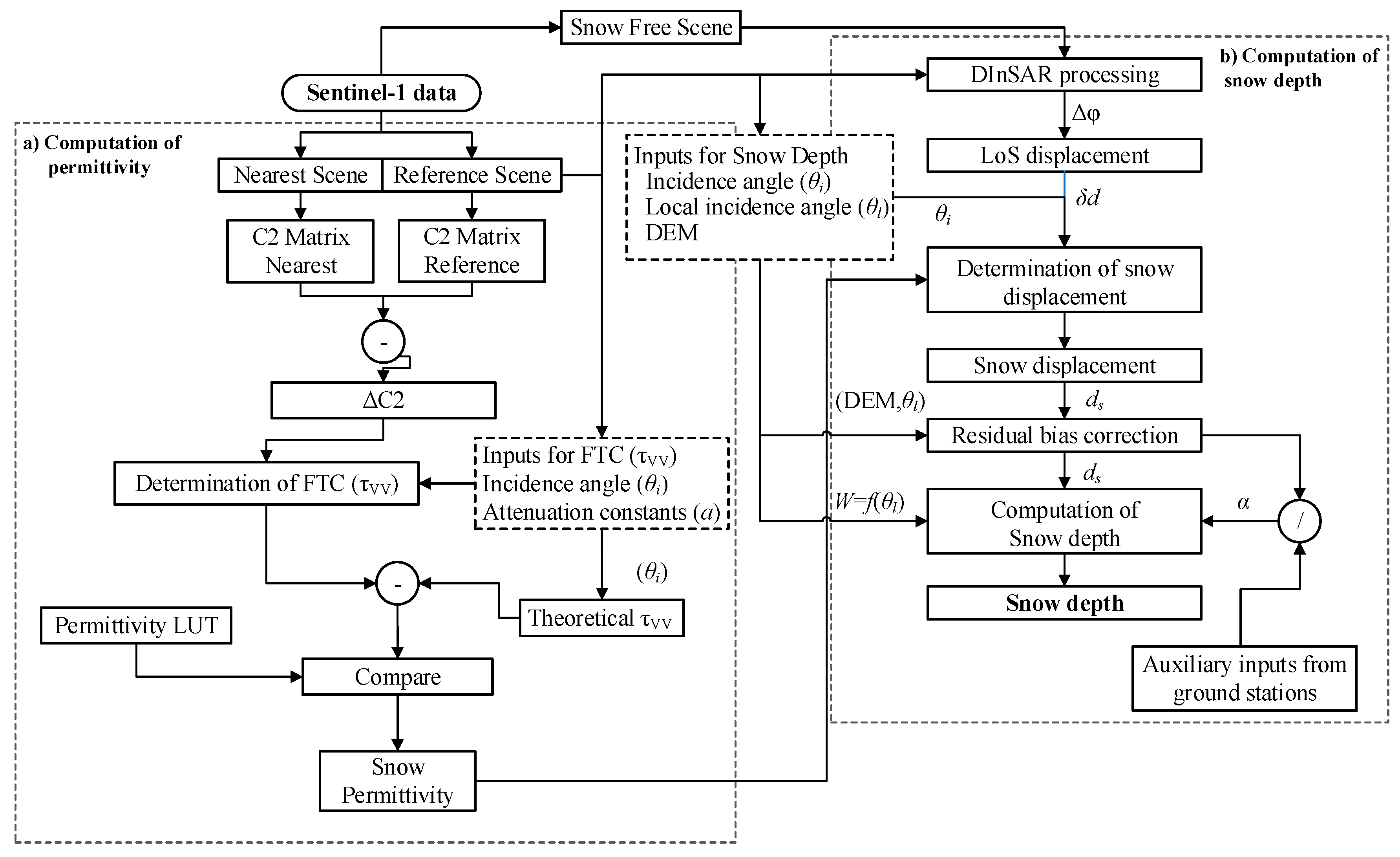
The proposed methodology includes; (1) the interferometric processing of the Sentinel-1 dual polarimetric SAR data (see Section 3.2) for the retrieval of DInSAR displacement, (2) the processing of the backscatter for deriving the snow permittivity (see Section 3.3) for the modeling of snow depth. The interferometric processing was used to estimate the preliminary displacements in the VV and VH channels. These displacements are improved by accounting for the effect of snow by introducing a correction for the snow permittivity. Additionally, we apply the bias corrections for the residual errors, as defined in Varade et al. [23]. The details of DInSAR processing, the snow phase model and the proposed method for incorporating the estimated snow permittivity for the corrections of the line of sight (LOS) displacements are explained in the following subsections. We applied masks to account for the layover shadow, SCA, and the local incidence angle to the modeled snow depth. The SCA was determined by thresholding the Normalized Difference Snow Index (NDSI), and the appropriate range of the local incidence angle is determined using the normal probability plot. The procedure for the generation of these masks is further explained in Section 4.1.
3.2. DInSAR Processing
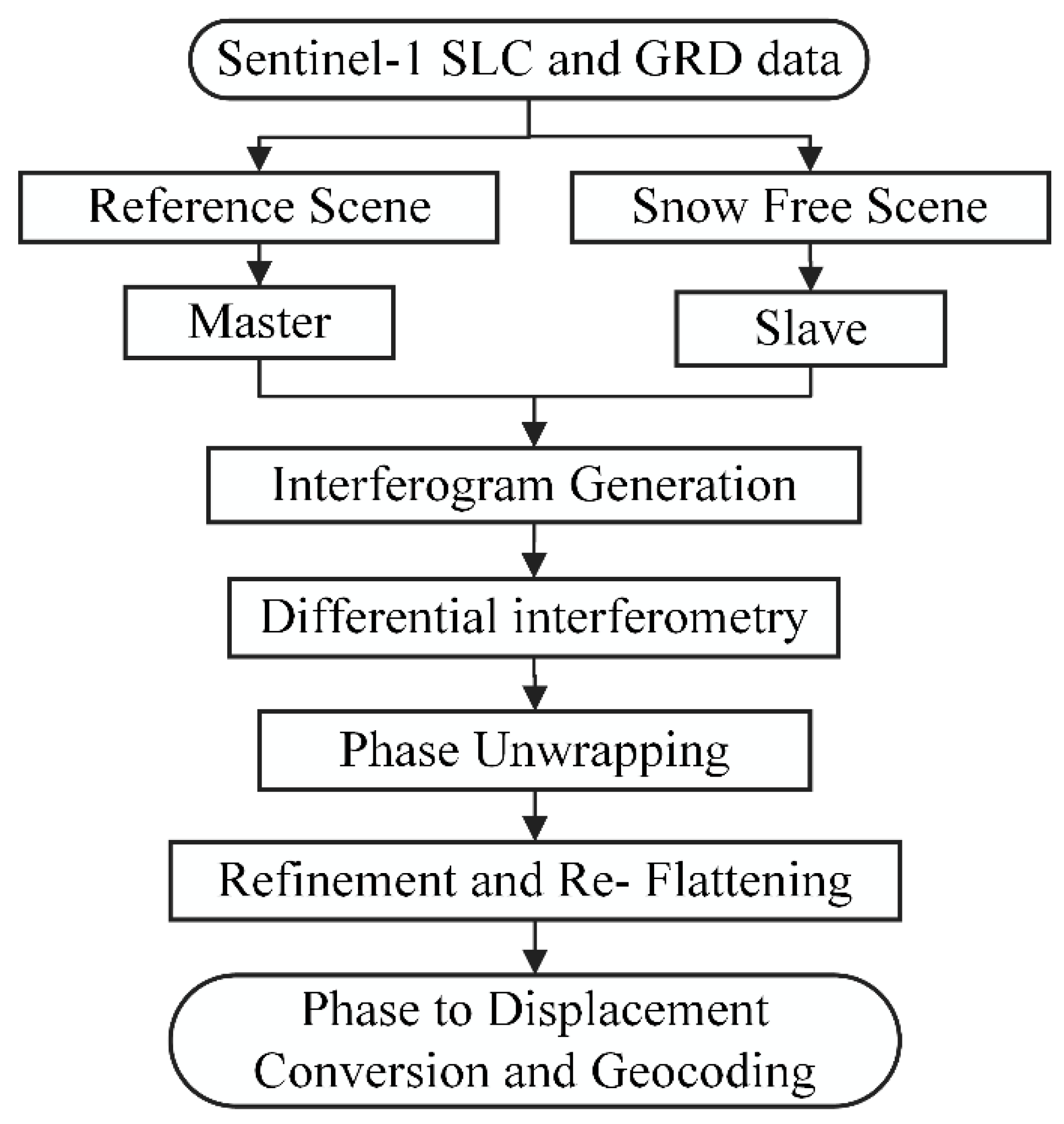
The DInSAR processing of the interferometric SAR (InSAR) data, as shown in Figure 3, can provide us with an estimate of the overall displacement of the incident surface in the line of sight (LOS) of the sensor. The quality of the differential interferograms is substantially influenced by the topography of the surface and the geometric configuration of the satellite orbit. A substantial advantage for the Sentinel-1 data over other interferometric radar data is the availability of the precise orbit information. In this study, a snow-free Sentinel-1 scene (i.e., 20 September 2018) was set as the master, and the snow-covered scenes of February and March 2019 were set as the slave to constitute the two pairs for DInSAR processing. The slight variations in the atmospheric conditions considerably affect the properties of snow. Snow is considered as a non-stationary medium, which causes a noticeable decrease in the coherence between the snow-free and the snow-covered scenes [23].
A critical factor in SAR interferometry is the baseline estimation, where efforts are made to ensure that the baseline is maintained within the critical limit [27]. A poor baseline usually results in the loss of interference, and subsequently, lower precision of the interferometric phase [17]. The interferogram and the coherence map were generated using two Sentinel-1 SLC master and slave images as defined previously [28]. The coherence value represents the ratio for the temporal correlation of master and slave SAR acquisition, which ranges between 0 and 1 [28]. Since snow is an incoherent material, the coherence for the snow-covered area is relatively low. The Shuttle Radar Topography Mission (SRTM) 1 arcsec (30 m) digital elevation model (DEM) is re-projected to the geometry of the master image for removing the topographic phase component and the output was regenerated as a slant range output product [29]. The interferogram was filtered using the Goldstein adaptive filter. To perform phase unwrapping, the maximum cost flow method was utilized. Refinement and re-flattening were implemented for the correct transformation of the unwrapped phase to the LOS displacement or height [29]. Moreover, this process enables us to refine the orbit information for possibly correcting the inaccuracies by calculating the phase offset and or removing the possible ramps [30]. The processed unwrapped phase was calibrated and converted to the displacement corresponding to the Geographic World Geodetic System 1984 (WGS84) datum map projection. Besides the displacement for each pixel, the location of northing and easting in the aforementioned geodetic reference system was retrieved using the geocoding [27].To perform the terrain correction for the estimated LOS displacement, the Range-Doppler method was applied [31].
Background on the Estimation of Snow Depth
Based on repeat-pass InSAR theory of the observed phase values, ϕ1 and ϕ2 with two observations taken at different times of the two images for a resolution cell are given as follows [20].
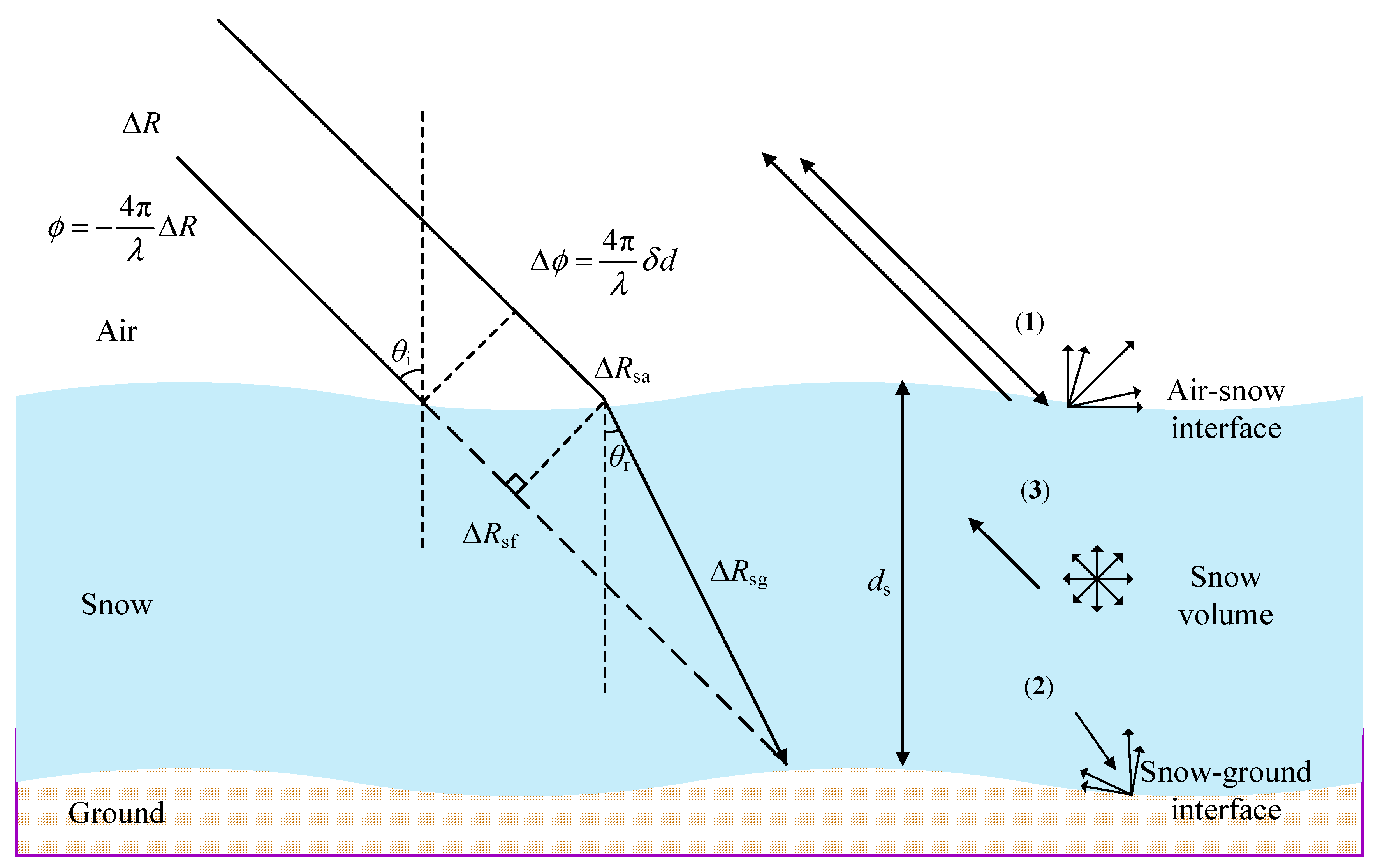
where R is the slant range distance, R + ΔR are the radar range distances, λ is the radar wavelength, and n1 and n2 are the contributions of the scattering phases in both the images, as shown in Figure 4, modified after Varade et al. [23]. Assuming that the characteristics of the scattering phases are equal during the two acquisitions, i.e., n1 = n2, mathematically, the interferometric phase ϕ can be determined as follows [18].
where ΔR is the one-way range difference. Equation (3) shows that the interferometric phase is proportional to the two-way range difference ΔR, which can be approximated as [32].
where B is the length of the baseline vector, which connects the two passes, and is the baseline component parallel to the radar look vector. During the image acquisition, if there are any changes in the incident target surface, the interferometric phase records the displacement of the surface along the radar LOS, which occurred during the acquisition of two (master and slave) images. The range difference between the two images are approximated as following [19]:
The residual phase Δϕ is obtained by subtracting the phase due to the flat earth and due to the topography. The residual phase corresponds to the surface deformation and the changes in electromagnetic properties along the propagation path, and is derived as follows [19]:
where δd indicates the radar LOS displacement.
For a nonmoving pixel, the radar wave range is shown as ΔRs without snow cover, and ΔRsa+ is shown with snow due to the refraction of the radar beam in the snow-air interface (1). The range difference is then represented by
At the snow-air interface, the incident radar wave undergoes refraction due to the difference in the dielectric properties of the air and the snow medium, which results in a corresponding phase shift [20]. Considering the snowpack to be dry, the backscatter from the snow-ground interface (Figure 4(2)) is exceedingly dominant over the component from the volume scattering (Figure 4(3)). [20]. For all types of dry snow (fresh, old, or wind-pressed snow, depth hoar, and refrozen crusts), the permittivity εs of dry snow is a function of snow density ρ only. The relationship between the snow permittivity and snow density can be represented by εs = 1 + 1.6ρ + 1.86ρ3, and the refraction index, n, is εs = n2 [33]. The snow phase ϕ shows the difference in the two-way propagation with snow-free and snow cover scenes and can be derived as follows [7,34],
3.3. Approximation of Snow Depth
As discussed earlier, the snow volume scattering influences the DInSAR phase, which is a function of the LOS displacement, incidence angle, and the snow permittivity [18]. For undisturbed and homogenous dry snow, either fresh or old, the permittivity of dry snow is a function of the snow density only. Thus, the snow phase, in this case, is represented by Equation (9) [18]. As mentioned earlier, the volume scattering effect for fresh snow is small. However, for old snow as observed in the peak winter and early melt season, the volume scattering is relatively dominant in the old snowpack as compared to the fresh snow [20]. Additionally, in the early melt season, the old snowpack may also exhibit the presence of LWC [33].
However, in this study, we do not have specific information on the presence of LWC of snow. From the available field observations, it was inferred that the first precipitation event of the winter season in 2019 occurred in January. After that, several snowfall events occurred. Considering that the initial accumulation of snow was substantially greater than that near the acquisition period of the Sentinel-1 data, the snowpack can be assumed to be relatively old. However, for the applicability of the aforementioned snow phase model, the snowpack should be dry, which is rarely the case in mountainous regions. The old snow in mountainous regions undergoes considerable melt and re-frost cycles, which often lead to the presence of some LWC in the snowpack. The refreeze processes cause snow compaction, affecting the [28] now density, which is a function of the snow permittivity [33]. Thus, in this study, we utilize the effective permittivity for modeling the snow depth from the DInSAR displacements, instead of utilizing the snow density as in [23]. Introducing the effect of the volume scattering in the snow on the LOS displacement leads to the following relation, which can be deduced from Equations (7) and (9) [35].
In Equation (10), we have two unknown variables, i.e., snow displacement, and snow permittivity. The snow permittivity is derived using the method defined by Varade et al. [36,37]. This method utilizes bi-temporal polarimetric radar data. In this study, we utilize the Sentinel-1 bi-temporal VV channel data for the estimation of snow density, due to the lack of fully polarimetric SAR data corresponding to the field campaigns. Varade et al. [37] investigated the capability of Sentinel-1 data for the modeling of snow permittivity and snow density. They observed the results based on Sentinel-1 data to be competitive with fully polarimetric decomposition-based methods.
In the literature [38,39,40,41], the snow permittivity has been derived from the Fresnel Transmission Coefficients (FTC). The theoretical relation between the FTC and the permittivity for the VV channel is defined in Equation (11). The method proposed by Varade et al. [37] utilizes the 2 × 2 covariance matrix elements to represent the incremental/decremental VV backscattering factors of the total modified Mueller matrix. These factors and the attenuation constants are used for the determination of the FTC, as shown in Equation (12). In Equation (12), C11 corresponds to the VV component of the reference scene covariance matrix. Subsequently, ΔC11 corresponds to the difference of the VV component of the reference and nearest scene covariance matrices, and a is the attenuation constant. The attenuation constants are determined by assuming exponential decay of the radar signal within the snowpack volume from the radar range Equation for the VV channel [37]. For the inversion of the permittivity from the FTC, we follow the widely used lookup table (LUT) based method. The LUT based method for the inversion of permittivity compares the theoretical (Equation (11)) and the estimated (Equation (12)) values of the FTC, such that permittivity from the LUT corresponding to the minimum error is selected. The workflow for the computation of the snow permittivity is shown in Figure 5a). Further details regarding the parameters and their tuning associated with this method are discussed in Section 4.2.
We followed the process for the determination of snow depth from the snow displacements, as defined in Varade et al. [23] and illustrated in Figure 5b). The residual bias correction is applied based on the zero gradient pixels identified from the 30 m SRTM 1 arcsec Digital Elevation Model (DEM), which is resampled to the spatial resolution of Sentinel-1 snow displacement rasters. The residual bias correction is carried out for the snow displacement in both the VV and the VH channels. The snow depth ( is determined as the scaled weighted sum of the snow displacements in these two channels, as shown in Equation (13), where the weights (W) are computed from the local incidence angle θl, as shown in Equation (14). The lower and upper bounds for the local incidence angle, and , respectively, were defined based on the normal probability plots for the two datasets (see Section 4.1). For the scale adjustment, we utilize the information on the snow accumulation derived from the total precipitation records available from the ground stations nearest to the field measurement sites. Specifically, these records were obtained from the Kalafgan and the Worsaj ground stations for both February and March 2019. The ratio of the mean accumulation depth of the snowpack and the mean corrected snow displacement is considered as the scale adjustment parameter α (Equation (15)).
4. Results
The experiments for the estimation of snow depth were carried out using the Sentinel-1 datasets (Table 1). The reference snow cover scenes for the estimation of the snow depth were selected based on the availability and the minimum difference in days from the date of field acquisitions. The datasets of February and March 2019 were selected for the snow-covered scenes with the minimum difference in days of 5 and 4, respectively, from the field measurements. In the DInSAR processing, the phase unwrapping via minimum cost flow was conducted with the pyramid levels, and the coherence threshold of 3 and 0.2, respectively [41]. The DInSAR processing was carried out in ENVI 5.5.3 with SARscape 5.5.2.1 (Harris Geospatial Pvt. Ltd.). The snow displacement estimation and corrections for the determination of snow depth were carried out in the MATLAB environment (MathWorks version 2018a).
4.1. Masking for SCA and Layover-Shadow Pixels
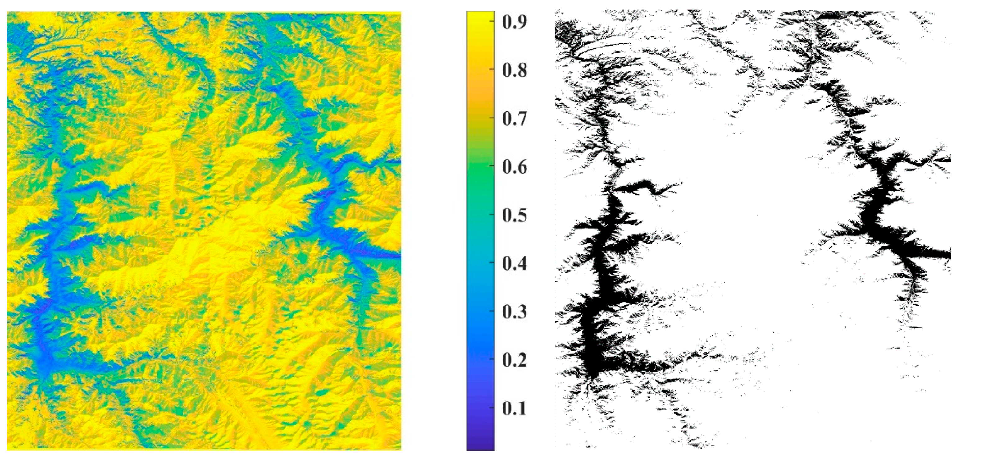
Since the study area is located in the high mountains of Pamir Hindu Kush, it is challenging to get cloud-free images, especially in the winter season. Unfortunately, due to the extensive cloud cover during the period of field campaigns, we could not find any freely available multispectral data (Landsat-8, Sentinel-2) for the determination of the SCA. Only one Landsat-8 scene in February 2019 in the vicinity of the target Sentinel-1 snow-covered scenes was available, which was used to determine the SCA. For the March 2019 dataset, we used the same SCA, as it was the only available Landsat-8 dataset (2 August 2019). The SCA was determined by thresholding the Normalized Difference Snow Index (NDSI) derived from the Level-2 Landsat-8 data product. Figure 6 illustrates the NDSI image and the corresponding SCA determined as NDSI > 0.4. Typically, the SCA is derived by thresholding the NDSI with thresholds selected in the range of 0.5–0.7 [42] For mixed snow/heterogenous/contaminated snow the NDSI values could be lower around 0.4 [43]. In this study, we observed the NDSI in the vicinity of the field campaign sites to be between 0.4–0.5. Thus, a lower threshold was selected such that the field campaign site is included in the SCA.
The total investigation area in this study comprises 6129 km2, i.e., 4951 × 5502 pixels for the target Sentinel-1 Single Look Complex (SLC) datasets. However, it is understandable that not all of these pixels are available for investigation due to the missing information on account of the layover shadow and the inconsistencies introduced by the local incidence angle. Thus, the total valid pixels for the study include those in the snow cover and outside layover shadow within the tolerable local incidence angle. It is observed that the local incidence angle has a substantial influence on the properties of the returned backscatter. The surface resolution for lower local incidence angles reduces sharply, and the signal to noise ratio for wet snow is substantially lower for the higher local incidence angles [44,45].
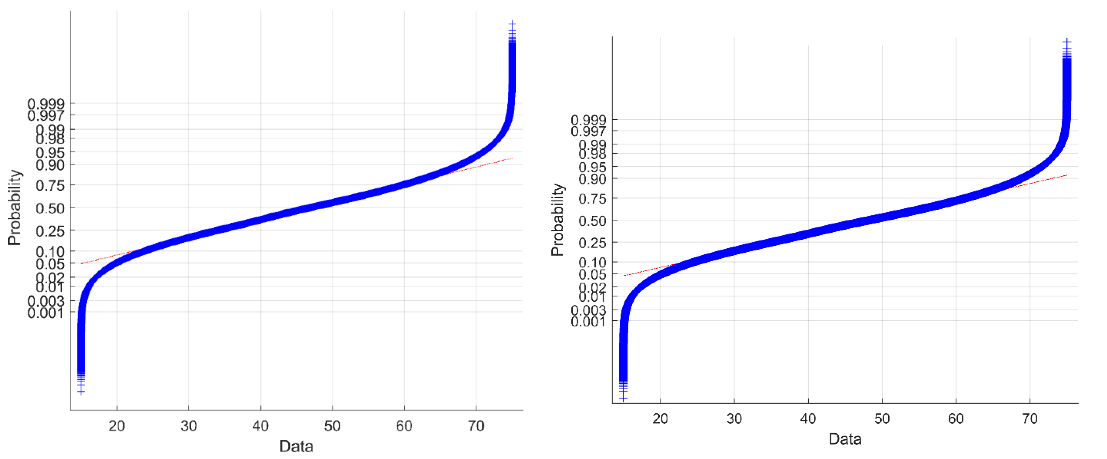
Additionally, in the mountainous regions at higher slopes, the DEM errors for near grazing angles have a higher possibility. Thus, to account for these issues, limiting the local incidence angle to an appropriate range for the investigations is highly recommended. In this case, the limits for the local incidence angle, i.e., the lower and the upper bounds, 15 and 75 degrees, respectively, for Equation (14), are determined from the observation of the normal probability plot of the local incidence angle shown in Figure 7 [17,20]. Table 2 summarizes the information available for investigation in the context of the number of pixels available for analysis on the SCA, layover shadow, local incidence angle mask, and the overall mask for the February and March 2019 datasets.
4.2. Spatial Distribution of the Snow Permittivity and Snow Depth
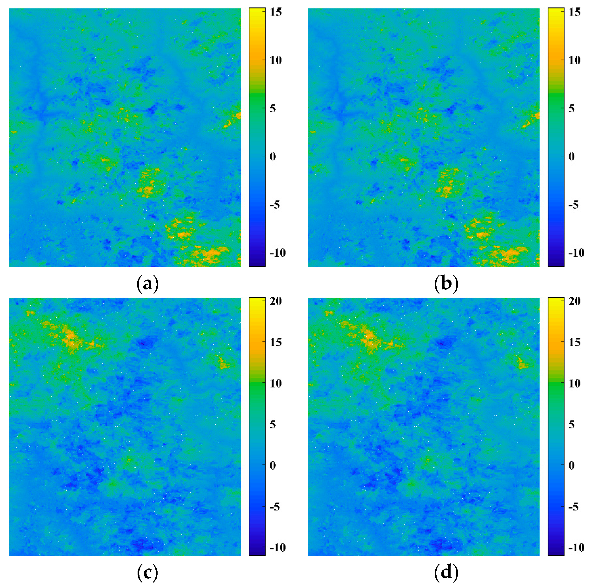
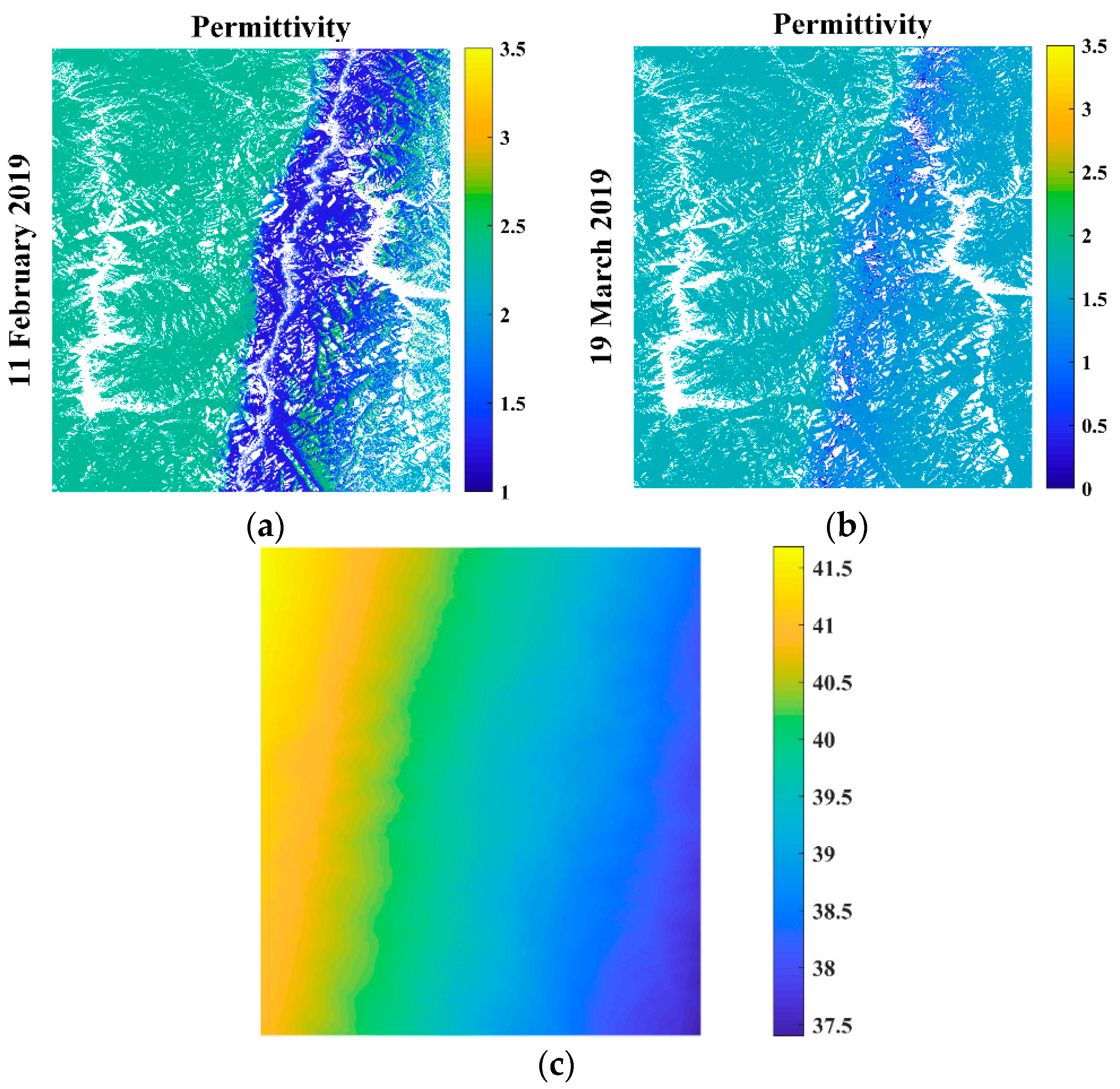
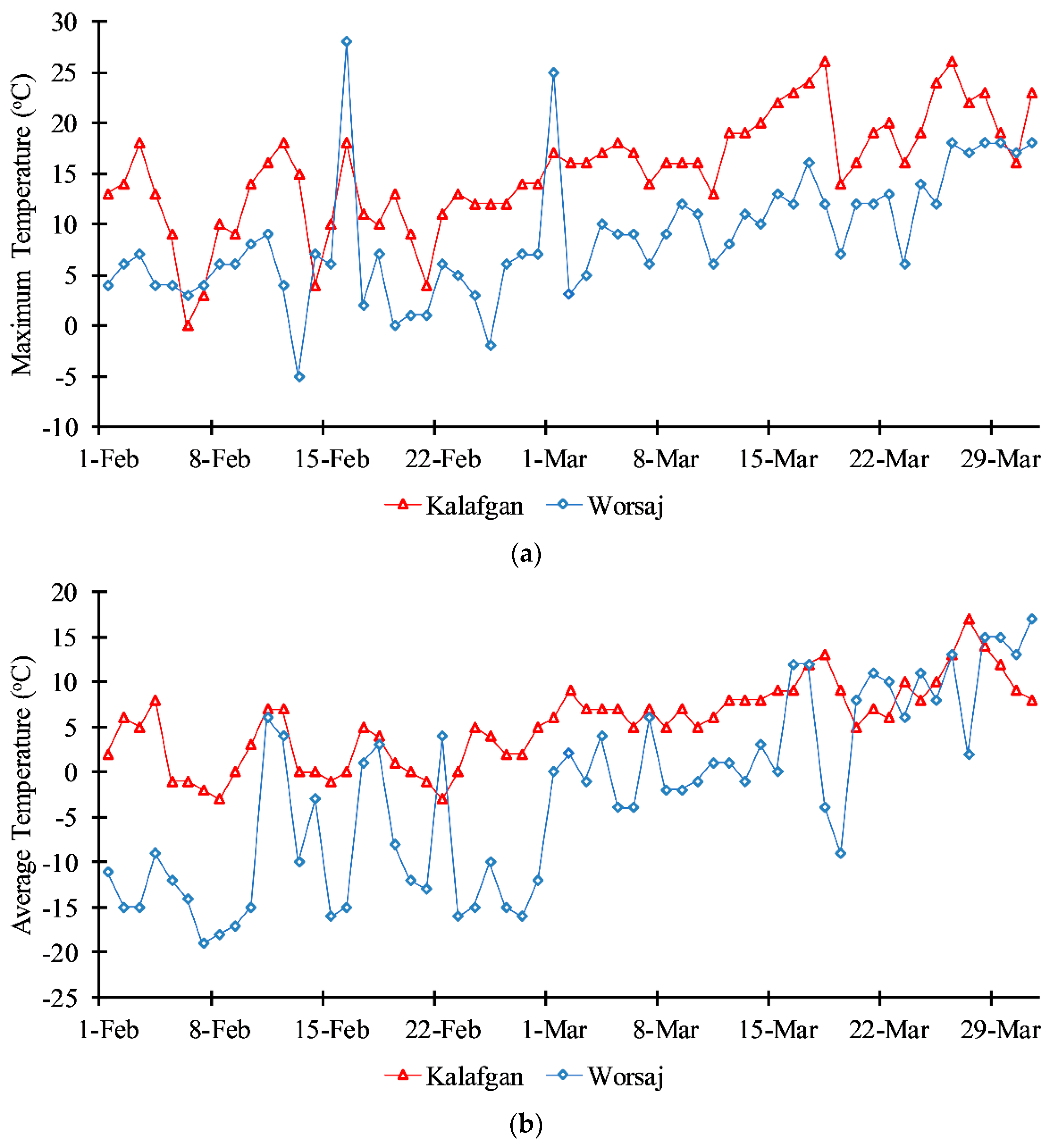
The different DInSAR LOS displacement maps for the months of January and February 2019 for the VV and the VH polarization channels are shown in Figure 8. Figure 9a,b, show the spatial distribution of the estimated snow permittivity for the February and the March 2019 datasets, respectively. It is observed that the western regions of the study area around Kalafgan have a relatively higher snow permittivity than expected for both February and March 2019, this is due to a discrepancy in the observed incidence angle for the Sentinel-1 datasets and the temperature variations as shown in Figure 10. It is worth mentioning that the incidence angle usually varies around 1–2° for the Sentinel-1 datasets from near range to far range. However, in this case, the range of the incidence angle is relatively higher, as observed in Figure 9c. This affects the computation of the theoretical FTC, which further influences the minimum error derived between the theoretical and the estimated FTC. Subsequently, the snow permittivity selected based on the LUT is also affected. This effect is more prominent in the February dataset where the snow is expected to be dry, while in March, the distribution of snow permittivity is relatively uniform throughout the study area. A possible reason for this could be the introduction of the snow LWC in the snowpack due to increasing temperatures in the temporal vicinity of 19 March 2019, as shown in Figure 11, which may have affected the backscatter. In this case, the snow permittivity is not only the function of snow density but also the LWC in the snowpack. However, in this study, we have limited the LUT for permittivity for old snow. Old snow exhibits a snow density of 0.20–0.45 g cm−3 [46,47] corresponding to the snow permittivity of 1.2–1.9, according to Mätzler’s relation [37,38,39]. Due to the lack of field observations, it is not possible to validate the estimates of the snow permittivity.
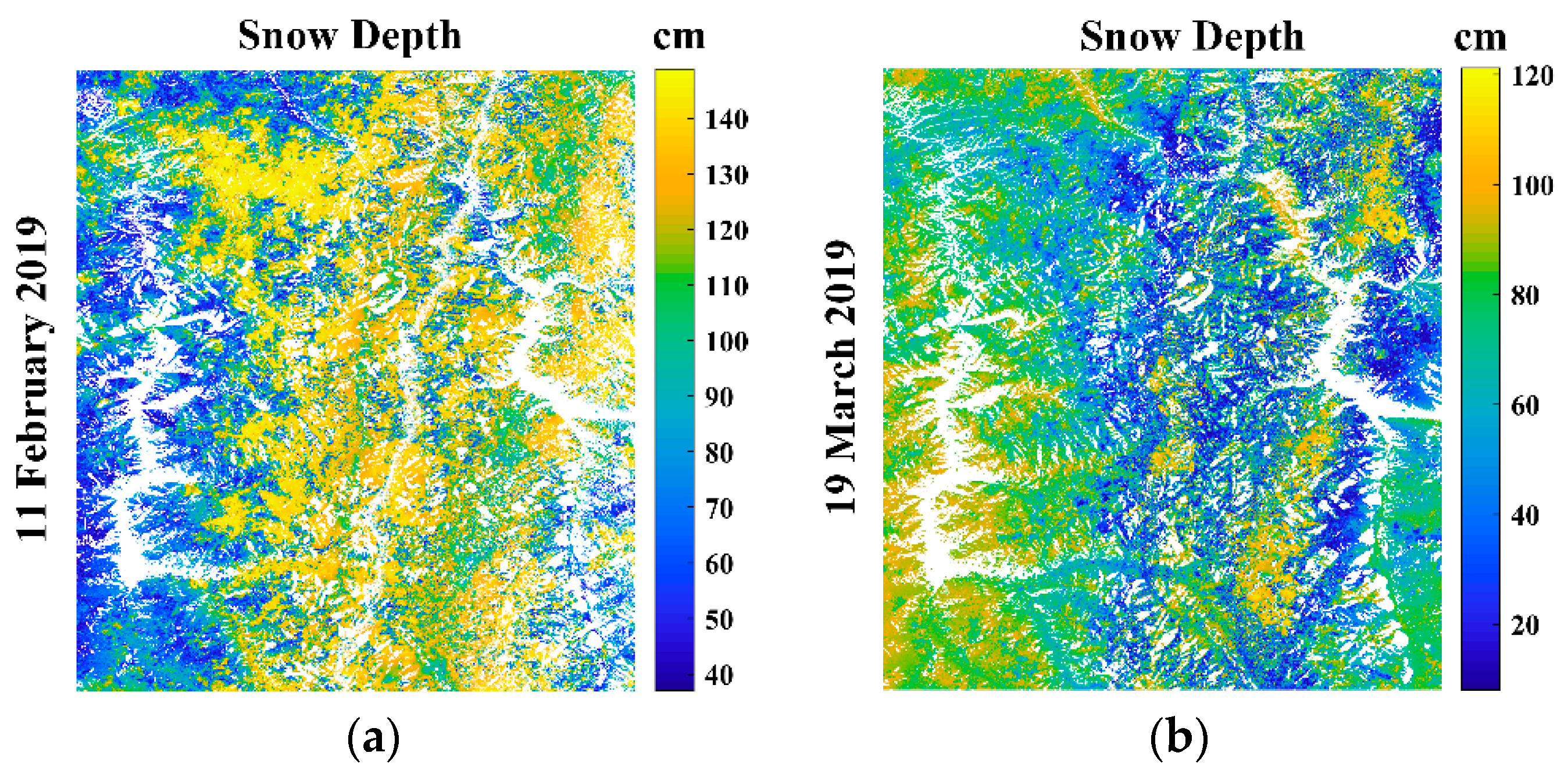
The spatial distribution of snow depth is shown in Figure 11a,b, for the February and March 2019 datasets. The results of February indicate that snow depth is higher than that of March 2019, which is expected in the regions of the Hindu Kush, where the peak snow depth is observed in the mid-end of February. The reduction of the snow depth in March 2019 could be attributed to the early snowmelt. Table 3 illustrates the retrieved snow permittivity and snow depth using the proposed approach for some of the prominent locations in the study area (see Figure 1). The elevation of the various locations also substantially affects the local weather and precipitation. Overall, the spatial distribution of the snow follows an expected trend with higher snow permittivity in the low-lying areas and vice versa for higher elevation areas. An inverse trend is observed for the snow depth expectedly, following greater depth in high elevation areas. An exception is noticeable at the Namakab station in the March dataset that shows uncharacteristic snow depth value. However, the Namakab station is located in a valley area surrounded on three sides by mountain slopes. Considering the geography and the geometry of the slopes leading to this area, it is possible that snow from the slopes drifted into this area due to wind.
In general, the spatial distribution of snow permittivity and snow depth along the Khanabad watershed of the Pamir ranges of the Hindu Kush in northern Afghanistan is characterized by the peak snow and melt season. The snowfall begins in early January in this region. Usually, the maximum depth of the snowpack is achieved at the end of February. Until mid-February in the study area, the snow type is usually dry due to consistently low temperatures in the peak winter season. In contrast, a higher temperature variation is observed in March, which signifies the beginning of the melt season near the end of this month. In general, for February, the snow is old and mostly dry, while in March, the snowpack tends to exhibit some LWC due to the gradual increase in melting. In summers, in April, and afterward, the snow becomes substantially wet [34]. Due to a lack of in-situ observations of snow liquid water content, we are unable to investigate the effect of the presence of moisture in the snowpack on the estimation of the snow depth. As we move towards the spring season, the diurnal temperature gradients tend to increase, causing a substantial melt and refreeze. This process causes polygranular grains of snow after periodical cycles of melt and refreeze, where the fraction of liquid water is not as considerable as the wet snow [44,45]. However, these results increase in the average snow density of the snowpack. The majority of the snowfall events occur during the months of January–March in the Hindu Kush region. Therefore, in general, in February and March, the snowpack is typically old [46]. In the literature, for the estimation of snow depth or the snow water equivalent, typically, the snowpack is assumed to be dry and or old [21,26,47]. The snow phase is related to the differential interferometric phase as well as the snow permittivity [20], or the snowpack snow density in the case of dry snow [19]. However, the incorporation of the snow permittivity and the snow density is corresponding to the volume scattering in the snowpack, considering it to be old and dry. In the case of wet snow, the permittivity is substantially higher than dry snow, and the surface scattering is dominant. In this case, the snow phase relations discussed previously would be rendered not applicable [36]. Subsequently, comprehensive studies on the estimation of snow depth for the case of wet snow are yet to be explored.
In this study, snow permittivity was determined using the method proposed by Varade et al. [23], which uses bi-temporal polarimetric SAR data. However, in the present case, the horizontal transmit-horizontal receive channel (HH channel) that is relatively more sensitive for snow properties is not available with the Sentinel-1 dataset [34] Furthermore, for the study area, an issue was encountered regarding the repeatability of the Sentinel-1 data during February and March 2019. Typically, the repeatability is 6–7 days over the other regions of Himalayas. However, for the study area, the nearest scene before the reference snow cover scene was 12 days before for March and <1 day before for February 2019. These gaps are either too large or too small with respect to the temporal baseline described in the methodology proposed in [23]. For the February dataset, we had to utilize the scenes of the opposite look directions, which may have resulted in some errors at the locations of higher local incidence angle, as indicated in Varade et al. [23] Further, in the 12 days gap between the reference and the nearest snow cover scene for the March 2019 dataset, there were several snowfall events, indicating a substantial change in the snowpack. This is possibly one of the factors that influenced the snow permittivity estimation for the March dataset. Another noteworthy issue is the possible effect of the presence of LWC in the snowpack on the estimation of the snow permittivity and the snow depth.
4.3. Accuracy Assessment of the Modeled Results
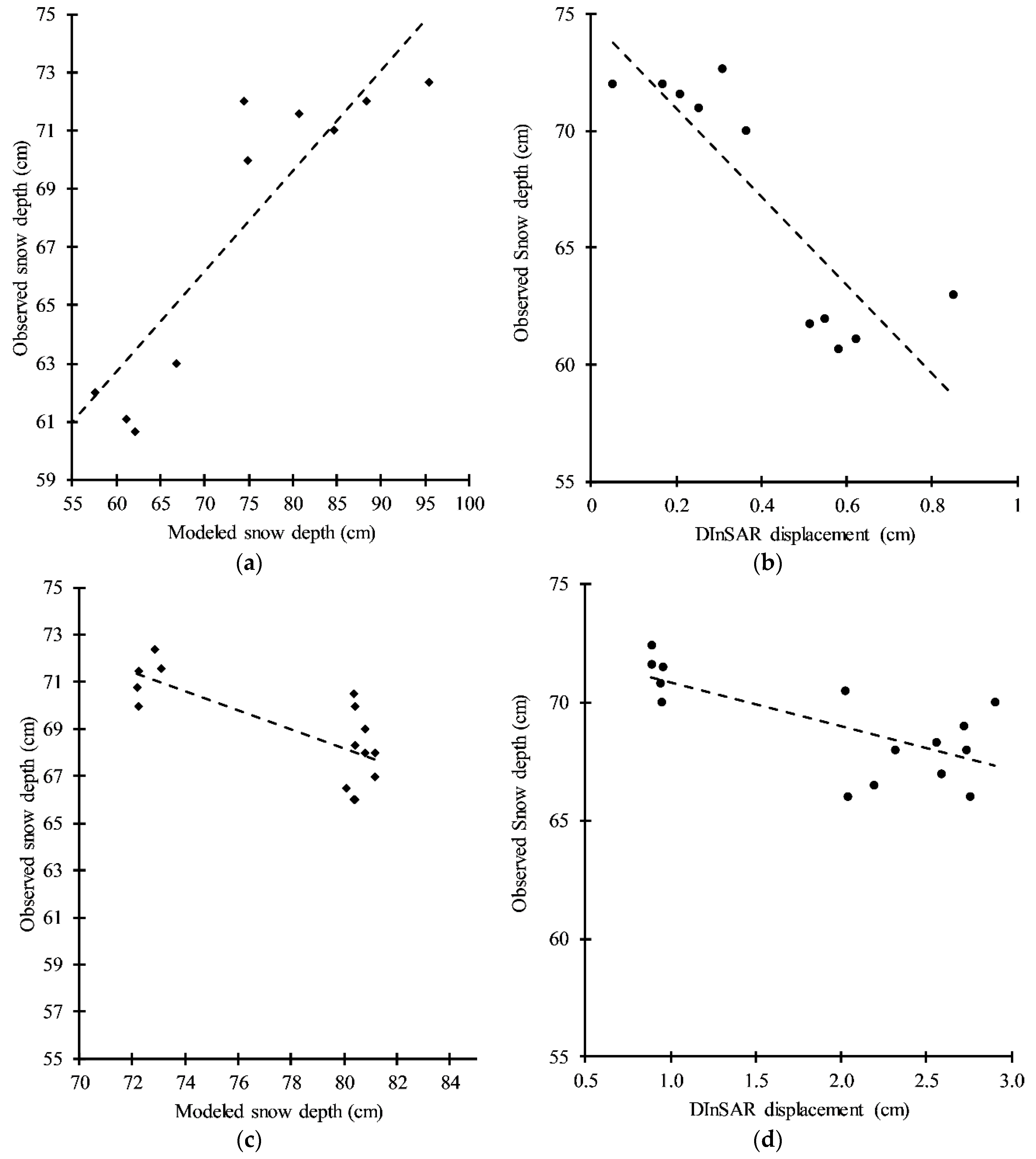
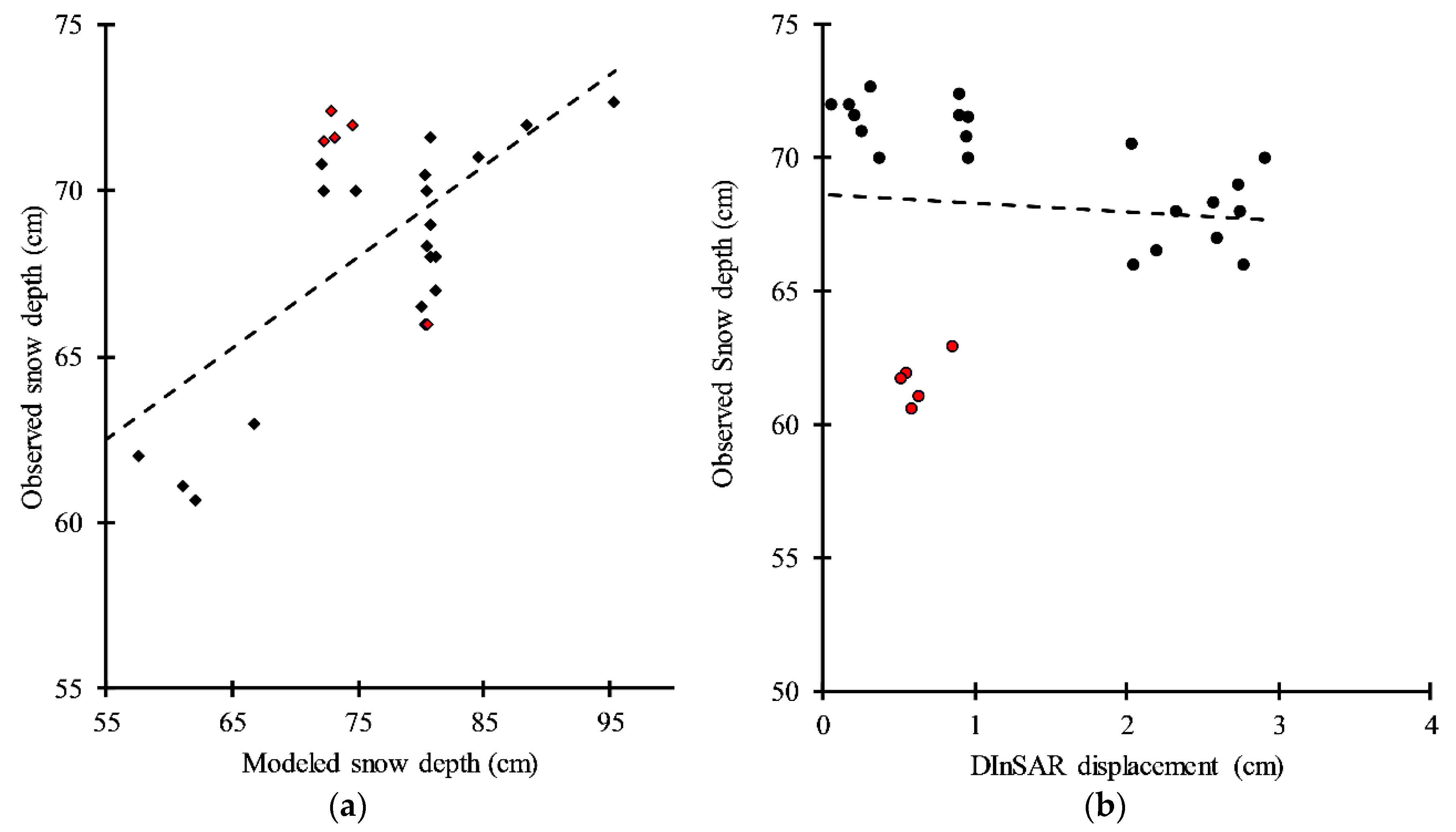
To evaluate the results of the proposed method, a comparison between the field measurements of snow depth with uncorrected two-pass DInSAR snow displacement and the corrected modeled snow depth was carried out for the accuracy assessment. The DInSAR displacement in this subsection refers to the mean of the DInSAR LOS displacement in the VV and the VH channels. Figure 12 and Figure 13 show the correlation plots for the accuracy assessment. The field measurements were carried out at distances of 2 m at the field site. However, the spatial resolution of the Sentinel-1 data after terrain correction was observed to be 15 m. Thus, any multiple field measurements corresponding to the same specific pixel were averaged out.
The accuracy assessment was carried out using the statistical parameters such as the coefficient of determination (R2), adjusted coefficient of determination (Adj R2), root mean square error (RMSE), mean square error (MSE), and the mean absolute error (MAE). Table 4 summarizes these statistical parameters for the February and March 2019 datasets. It is observed that the proposed method shows substantially better correlation and relatively lower error statistics with the field measurements as compared to the DInSAR displacement method. The DInSAR displacement, in this case, showed inferior results, possibly due to the presence of some outliers, as shown in red dots in Figure 13. Upon removing these points from the accuracy assessment, a considerable improvement in the estimated snow depth is observed. In this case, the observed values of (R2, Adj R2) were observed to be (0.7229, 0.7128), respectively, for the estimated snow depth. In general, it is observed that the mean absolute error is, in general, lower than 10 cm for the estimated snow depth, which is acceptable for a DInSAR based approach [48,49,50].
5. Conclusions
In this study, we analyzed the potential of Sentinel-1 dual polarimetric and interferometric observations for the estimation of snow depth in the Khanabad watershed of the Pamir ranges of the Hindu Kush Himalayas in Afghanistan. From the perspective of the water resources, the Khanabad watershed holds substantial impact as the primary contributor to the runoff in the Amu River. Thus, for the hydrological modeling in the Khanabad watershed, the proposed approach could be vital in improving the estimates of snow water equivalent, which is one of the key inputs in this regard. Additionally, the proposed approach is based on the freely available Sentinel-1 data utilizing multi-temporal dual polarimetric and interferometric SAR techniques. Subsequently, the proposed method may contribute to the continuous monitoring of the snowpack thickness.
In the proposed approach for the estimation of snow depth, the conventional DInSAR LOS displacements were improved by incorporating spatially distributed snow permittivity determined from the bi-temporal Sentinel-1 VV channel data. The snow depth was determined as the scaled weighted sum of the corrected displacements in the VV and the VH channels. As compared to the conventional DInSAR displacement, the proposed method showed significantly better accuracy with respect to field measurements. The R2/RMSE corresponding to all the field measurements with respect to DInSAR displacement and the proposed method were 0.007/3.9 cm and 0.48/2.8 cm, respectively. The lower R2, in this case, was attributed to the presence of some outliers.
It was observed that the estimated snow depth derived from the proposed method showed an excellent coefficient of determination (R2) of 0.82 versus field measurements for the peak winter season. Conversely, a relatively lower correlation with R2 of 0.57 was observed for the melt season. The lower correlation in the melt season could be attributed to; (1) inconsistencies in the snow permittivity estimation due to a lack of availability of suitable Sentinel-1 scenes, (2) possible effect of the presence of LWC in the snowpack, (3) issues related to looking angle of the Sentinel-1 scenes available for this study. However, the RMSE for the melt season (1.45 cm) was observed to be relatively smaller than that of peak winter (2.34 cm).
With future missions like the National Aeronautics and Space Administration (NASA)—Indian Space Research Organization (ISRO) SAR (NISAR), it might be possible to retrieve highly repeatable and consistent (incidence angle) data over the study area accounting for issues encountered for estimating snow permittivity, mainly related to the periodical difference in acquisition of the reference and nearest snow-covered scenes. The utilization of fully polarimetric and interferometric SAR data would be highly efficient for improving the snow phase model to better account for the fractional liquid water content in the snowpack. However, such data is commercial with on-demand availability and, thus, not suitable for the continuous monitoring of the snowpack, and efforts under these directions are left for future work.
Author Contributions
Conceptualization, A.B.M. and D.V.; Methodology, Mahmoodzada, D.V. and S.S.; Data collection, A.B.M.; Writing—original draft preparation, A.B.M.; Writing—review and editing, D.V. and S.S.; Supervision, S.S. and D.V.; Funding acquisition, S.S.; All authors have read and agreed to the published version of the manuscript.
Funding
This research was financially supported by the Project for Promotion and Enhancement of the Afghan Capacity for Effective Development (PEACE) of Japan International Cooperation Agency (JICA).
Acknowledgments
Authors acknowledge the General Affairs of Snow and Glacier Analysis, Department of Surface Water, General Directorate of Water Resources, National Water Affairs Regulation Authority (GMSGA), Afghanistan, for their assistance with snow depth filed measurement data and earth explorer portal of USGS and the Copernicus open access hub of ESA, which is freely accessible to the scientific community.
Conflicts of Interest
The authors declare no conflict of interest.
References
- Georgievsky, M.V. Application of the Snowmelt Runoff model in the Kuban river basin using MODIS satellite images. Environ. Res. Lett. 2009, 4, 045017. [Google Scholar] [CrossRef] [Green Version]
- Kulkarni, A.V.; Rathore, B.; Singh, S.; Ajai, U. Distribution of seasonal snow cover in central and western Himalaya. Ann. Glaciol. 2010, 51, 123–128. [Google Scholar] [CrossRef] [Green Version]
- Gurung, D.R.; Kulkarni, A.V.; Giriraj, A.; Aung, K.S.; Shrestha, B.; Srinivasan, J. Changes in seasonal snow cover in Hindu Kush-Himalayan region. Cryosphere Discuss. 2011, 5, 755–777. [Google Scholar] [CrossRef] [Green Version]
- World Bank. Europe and Central Asia: Assessment of the Role of Glaciers in Stream Flow from the 564 Pamir and Tien Shan Mountains; The World Bank: Washington, DC, USA, 2015. [Google Scholar]
- Klemm. Impact of Irrigation in Northern Afghanistan on Water Use in the Amu Darya Basin Walter. 2009. Available online: https://www.unece.org/fileadmin/DAM/SPECA/documents/ecf/2010/FAO_report_e.pdf (accessed on 6 March 2020).
- Agal’Tseva, N.A.; Bolgov, M.V.; Spektorman, T.Y.; Trubetskova, M.D.; Chub, V.E. Estimating hydrological characteristics in the Amu Darya River basin under climate change conditions. Russ. Meteorol. Hydrol. 2011, 36, 681–689. [Google Scholar] [CrossRef]
- Kinar, N.J.; Pomeroy, J.W. Reviews of Geophysics Measurement of the physical properties of the snowpack. Rev. Geophys. 2015, 53, 481–544. [Google Scholar] [CrossRef]
- Ulaby, F.; Long, D.; Blackwell, W.J.; Elachi, C.; Fung, A.K. Microwave Radar and Radiometric Remote Sensing; The University of Michigan: Ann Arbor, MI, USA, 2014. [Google Scholar]
- Dong, C. Remote sensing, hydrological modeling and in situ observations in snow cover research: A review. J. Hydrol. 2018, 561, 573–583. [Google Scholar] [CrossRef]
- Varade, D.; Dikshit, O. Potential of multispectral reflectance for assessment of snow geophysical parameters in Solang valley in the lower Indian Himalayas. GIScience Remote Sens. 2019, 57, 107–126. [Google Scholar] [CrossRef]
- Varade, D.; Dikshit, O. Estimation of surface snow wetness using sentinel-2 multispectral data. ISPRS Ann. Photogramm. Remote Sens. Spat. Inf. Sci. 2018, 4, 223–228. [Google Scholar] [CrossRef] [Green Version]
- Che, T.; Li, X.; Jin, R.; Armstrong, R.; Zhang, T. Snow depth derived from passive microwave remote-sensing data in China. Ann. Glaciol. 2008, 49, 145–154. [Google Scholar] [CrossRef] [Green Version]
- Dozier, J.; Shi, J. Estimation of snow water equivalence using SIR-C/X-SAR. I. Inferring snow density and subsurface properties. IEEE Trans. Geosci. Remote Sens. 2000, 38, 2465–2474. [Google Scholar] [CrossRef] [Green Version]
- Vuyovich, C.; Jacobs, J.M. Snowpack and runoff generation using AMSR-E passive microwave observations in the Upper Helmand Watershed, Afghanistan. Remote Sens. Environ. 2011, 115, 3313–3321. [Google Scholar] [CrossRef]
- Deems, J.; Painter, T.H.; Finnegan, D.C. Lidar measurement of snow depth: A review. J. Glaciol. 2013, 59, 467–479. [Google Scholar] [CrossRef] [Green Version]
- Leinss, S.; Parrella, G.; Hajnsek, I. Snow height determination by polarimetric phase differences in X-Band SAR data. IEEE J. Sel. Top. Appl. Earth Obs. Remote Sens. 2014, 7, 3794–3810. [Google Scholar] [CrossRef] [Green Version]
- Patil, A.; Mohanty, S.; Singh, G. Snow depth and snow water equivalent retrieval using X-band PolInSAR data. Remote Sens. Lett. 2020, 11, 817–826. [Google Scholar] [CrossRef]
- Abe, T.; Yamaguchi, Y.; Sengoku, M. Experimental study of microwave transmission in snowpack. IEEE Trans. Geosci. Remote Sens. 1990, 28, 915–921. [Google Scholar] [CrossRef]
- Ferretti, A.; Monti-guarnieri, A.; Prati, C.; Rocca, F. Part C InSAR P Rocessing: A Mathematical Approach. 2007, p. 115. Available online: https://www.esa.int/esapub/tm/tm19/TM-19_ptC.pdf (accessed on 12 May 2020).
- Deeb, E.; Forster, R.R.; Kane, D.L. Monitoring snowpack evolution using interferometric synthetic aperture radar on the North Slope of Alaska, USA. Int. J. Remote Sens. 2011, 32, 3985–4003. [Google Scholar] [CrossRef]
- Li, H.; Wang, Z.; He, G.; Man, W. Estimating snow depth and snow water equivalence using repeat-pass interferometric SAR in the northern piedmont region of the Tianshan Mountains. J. Sens. 2017, 2017, 8739598. [Google Scholar] [CrossRef]
- Guneriussen, T.; Hogda, K.; Johnsen, H.; Lauknes, I. InSAR for estimation of changes in snow water equivalent of dry snow. IEEE Trans. Geosci. Remote Sens. 2001, 39, 2101–2108. [Google Scholar] [CrossRef]
- Varade, D.; Maurya, A.; Dikshit, O.; Singh, G.; Manickam, S. Snow depth in Dhundi: An estimate based on weighted bias corrected differential phase observations of dual polarimetric bi-temporal Sentinel-1 data. Int. J. Remote Sens. 2019, 41, 3031–3053. [Google Scholar] [CrossRef]
- Gámez, P.S.; Navarro, F. Glacier surface velocity retrieval using D-InSAR and offset tracking techniques applied to ascending and descending passes of sentinel-1 data for Southern Ellesmere Ice Caps, Canadian Arctic. Remote Sens. 2017, 9, 442. [Google Scholar] [CrossRef] [Green Version]
- Strozzi, T.; Antonova, S.; Günther, F.; Mätzler, E.; Vieira, G.; Wegmuller, U.; Westermann, S.; Bartsch, A. Sentinel-1 SAR interferometry for surface deformation monitoring in low-land permafrost areas. Remote Sens. 2018, 10, 1360. [Google Scholar] [CrossRef] [Green Version]
- Liu, Y.; Li, L.; Yang, J.; Chen, X.; Hao, J. Estimating snow depth using multi-source data fusion based on the D-InSAR Method and 3DVAR fusion algorithm. Remote Sens. 2017, 9, 1195. [Google Scholar] [CrossRef] [Green Version]
- Ahmad, M.; Wasiq, M. Water Resource Development in Northern Afghanistan and Its Implications for Amu Darya Basin; World Bank: Washington, DC, USA, 2004. [Google Scholar]
- Kamal, G.M. River Basins and Watersheds of Afghanistan. 2004, pp. 1–7. Available online: http://www.nzdl.org/gsdl/collect/areu/Upload/1710/Kamal_River basins and watersheds2004.pdf (accessed on 20 February 2020).
- Rucci, A.; Ferretti, A.; Monti-Guarnieri, A.; Rocca, F. Sentinel 1 SAR interferometry applications: The outlook for sub millimeter measurements. Remote Sens. Environ. 2012, 120, 156–163. [Google Scholar] [CrossRef]
- Sarmap. SARscape Help Manual. 2014. Available online: http://sarmap.ch/tutorials/Basic.pdf (accessed on 20 May 2020).
- Description, D.S. SARscape Interferometry Module for Displacement Map Generation SARscape Processing Steps Baseline Estimation Digital Elevation Model/Ellipsoid Interferogram Flattening; European Space Agency (ESA): Paris, France, 2004; Volume 2003, pp. 1–4. [Google Scholar]
- Lensu, T. Synthetic aperture radar—Systems and signal processing. Signal. Process. 1992, 29, 107. [Google Scholar] [CrossRef]
- Klemm, R. Novel Radar Techniques and Applications Volume 1: Real Aperture Array Radar, Imaging Radar, and Passive and Multistatic Radar; Institution of Engineering and Technology: London, UK, 2017. [Google Scholar]
- Simonetto, E. DINSAR experiments using a free processing chain. SPIE Remote Sens. 2008, 7109, 71091G. [Google Scholar] [CrossRef]
- Moreira, P.A.; Prats-iraola, M.; Younis, G.; Krieger, I.; Hajnsek, K.; Papathanassiou, K.P. AR-Tutorial-March-2013. IEEE Geosci. Remote Sens. Mag. 2013, 6–43. [Google Scholar] [CrossRef] [Green Version]
- Rosen, P.; Hensley, S.; Joughin, I.; Li, F.; Madsen, S.; Rodriguez, E.; Goldstein, R. Synthetic aperture radar interferometry. Proc. IEEE 2000, 88, 333–382. [Google Scholar] [CrossRef]
- Mätzler, C. Microwave permittivity of dry sand. IEEE Trans. Geosci. Remote Sens. 1998, 36, 317–319. [Google Scholar] [CrossRef]
- Rott, H.; Nagler, T.; Scheiber, R. Snow mass retrieval by means of SAR interferometry. Eur. Sp. Agency 2004, 550, 187–192. [Google Scholar]
- Singh, G.; Verma, A.; Kumar, S.; Snehmani; Ganju, A.; Yamaguchi, Y.; Kulkarni, A.V. Snowpack density retrieval using fully polarimetric TerraSAR-X data in the Himalayas. IEEE Trans. Geosci. Remote Sens. 2017, 55, 6320–6329. [Google Scholar] [CrossRef]
- Varade, D.; Manickam, S.; Dikshit, O.; Singh, G. Snehmani Modelling of early winter snow density using fully polarimetric C-band SAR data in the Indian Himalayas. Remote Sens. Environ. 2020, 240, 111699. [Google Scholar] [CrossRef]
- Varade, D.; Dikshit, O.; Manickam, S.; Singh, G. Snehmani Capability assessment of Sentinel-1 bi-temporal dual polarimetric SAR data for inferences on snow density. In Proceedings of the 2019 IEEE MTT-S International Microwave and RF Conference (IMARC), Mumbai, India, 13–15 December 2019; pp. 1–5. [Google Scholar] [CrossRef]
- Manickam, S.; Bhattacharya, A.; Singh, G.; Yamaguchi, Y. Estimation of snow surface dielectric constant from polarimetric SAR Data. IEEE J. Sel. Top. Appl. Earth Obs. Remote Sens. 2016, 10, 211–218. [Google Scholar] [CrossRef]
- Zhang, B.; Li, J.; Ren, H. Using phase unwrapping methods to apply D-InSAR in mining areas. Can. J. Remote Sens. 2019, 45, 225–233. [Google Scholar] [CrossRef]
- Choi, H.; Bindschadler, R. Cloud detection in Landsat imagery of ice sheets using shadow matching technique and automatic normalized difference snow index threshold value decision. Remote Sens. Environ. 2004, 91, 237–242. [Google Scholar] [CrossRef]
- Varade, D.; Dikshit, O.; Manickam, S. Dry/wet snow mapping based on the synergistic use of dual polarimetric SAR and multispectral data. J. Mt. Sci. 2019, 16, 1435–1451. [Google Scholar] [CrossRef]
- Nagler, T.; Rott, H.; Ripper, E.; Bippus, G.; Hetzenecker, M. Advancements for snowmelt monitoring by means of sentinel-1 SAR. Remote Sens. 2016, 8, 348. [Google Scholar] [CrossRef] [Green Version]
- He, Y.; Wetterhall, F.; Cloke, H.L.; Pappenberger, F.; Wilson, M.D.; Freer, J.E.; McGregor, G. Tracking the uncertainty in flood alerts driven by grand ensemble weather predictions. Meteorol. Appl. 2009, 16, 91–101. [Google Scholar] [CrossRef] [Green Version]
- Colbeck, S.C. Grain clusters in wet snow. J. Colloid Interface Sci. 1979, 72, 371–384. [Google Scholar] [CrossRef]
- Colbeck, S.C. An overview of seasonal snow metamorphism. Rev. Geophys. 1982, 20, 45–61. [Google Scholar] [CrossRef]
- Surendar, M.; Bhattacharya, A.; Singh, G.; Venkataraman, G. Estimation of snow density using full-polarimetric Synthetic Aperture Radar (SAR) data. Phys. Chem. Earth 2015, 83–84, 156–165. [Google Scholar] [CrossRef]
Figure 1.
Study area with annotated location of the field campaigns (Kalafgan and Worsaj) and other prominent locations in the Khanabad watershed of northern Afghanistan.
Figure 1.
Study area with annotated location of the field campaigns (Kalafgan and Worsaj) and other prominent locations in the Khanabad watershed of northern Afghanistan.

Figure 2.
Field photographs from the campaigns conducted by a survey team from General Affairs of Snow and Glacier Analysis, Department of Surface Water, General Directorate of Water Resources, National Water Affairs Regulation Authority (GMSGA), Afghanistan. The left image shows the ruler used for the measurement of the snow depth. Additional measurements were obtained from snow tubes, as shown in the right image.

Figure 3.
Flowchart for the generation of DInSAR line of sight (LOS) displacement.

Figure 4.
The geometry of the radar wave in dry snow, modified after Varade et al. [23]; (1) shows the geometry corresponding to the air-snow interface, (2) shows the refraction in the snow volume and the corresponding effect on the range, and (3) shows the range corresponding to the snow-free case.

Figure 5.
The detailed flowchart for the proposed method. Part (a) illustrates the computation of the snow permittivity, and part (b) shows the incorporation of the estimated snow permittivity in the modeling of snow depth.
Figure 5.
The detailed flowchart for the proposed method. Part (a) illustrates the computation of the snow permittivity, and part (b) shows the incorporation of the estimated snow permittivity in the modeling of snow depth.

Figure 6.
Normalized Difference Snow Index (NDSI) and the corresponding snow cover area (SCA).

Figure 7.
Normal probability plots for the snow-covered scenes of February and March 2019 in left and right, respectively. In the plots, the y-axis shows the normal probability and the x-axis refers to the data corresponding to the different values of the local incidence angle observed.
Figure 7.
Normal probability plots for the snow-covered scenes of February and March 2019 in left and right, respectively. In the plots, the y-axis shows the normal probability and the x-axis refers to the data corresponding to the different values of the local incidence angle observed.

Figure 8.
DInSAR LOS displacement in the VV and VH polarization; for 11 February 2019 (a,b), for 19 March 2019 (c,d), respectively, derived using the approach mentioned in Section 3.2.
Figure 8.
DInSAR LOS displacement in the VV and VH polarization; for 11 February 2019 (a,b), for 19 March 2019 (c,d), respectively, derived using the approach mentioned in Section 3.2.

Figure 9.
Estimated distribution maps of snow permittivity (a,b) and incidence angle (c) derived using proposed mythology for 11 February, and 19 March, 2019, Sentinel-1 dataset.
Figure 9.
Estimated distribution maps of snow permittivity (a,b) and incidence angle (c) derived using proposed mythology for 11 February, and 19 March, 2019, Sentinel-1 dataset.

Figure 10.
Maximum and mean daily temperatures of Kalafgan and Worsaj as determined from data available from AccuWeather Pvt. Ltd. for February and March 2019.
Figure 10.
Maximum and mean daily temperatures of Kalafgan and Worsaj as determined from data available from AccuWeather Pvt. Ltd. for February and March 2019.

Figure 11.
Spatial distribution of the estimated snow depth for 11 February 2019 (a) and 19 March 2019 (b), based on the proposed method using the Sentinel-1 datasets.
Figure 11.
Spatial distribution of the estimated snow depth for 11 February 2019 (a) and 19 March 2019 (b), based on the proposed method using the Sentinel-1 datasets.

Figure 12.
A comparison with respect to the field measurements for February and March 2019; modeled snow depth estimates using the proposed approach (a,c) and DInSAR based displacement (b,d), respectively.
Figure 12.
A comparison with respect to the field measurements for February and March 2019; modeled snow depth estimates using the proposed approach (a,c) and DInSAR based displacement (b,d), respectively.

Figure 13.
Correlation plots for the overall data, including February and March field measurement points for the estimated snow depth from the proposed method in (a) and DInSAR displacement in (b). The red points in both the plots show possible outliers.
Figure 13.
Correlation plots for the overall data, including February and March field measurement points for the estimated snow depth from the proposed method in (a) and DInSAR displacement in (b). The red points in both the plots show possible outliers.


Table 1.
Sentinel-1 C-band dual polarimetric and interferometric synthetic aperture radar (SAR) datasets were used in this study.
Table 1.
Sentinel-1 C-band dual polarimetric and interferometric synthetic aperture radar (SAR) datasets were used in this study.
| Month | February | Incidence Angle | March | Incidence Angle |
|---|---|---|---|---|
| Reference Snow Covered Scene | 20190211 | 43.76 | 20190319 | 43.77 |
| Nearest Snow-Covered Scene | 20190210 | 45.36 | 20190307 | 43.77 |
| Snow Free Scene | 20180920 | 41.99 | 20180920 | 41.99 |
| DInSAR Temporal Baseline | 144 days | 182 days |
Table 2.
The information for study investigation in terms of the number of pixels available for analysis.
Table 2.
The information for study investigation in terms of the number of pixels available for analysis.
| Months | Total Number of Pixels Per Image = 27,240,402 Total Investigation Area = 6129.09 km2 | |||||
|---|---|---|---|---|---|---|
| Data | Source | Date | Total No of Pixels | Percentage of Valid Pixels | Percentage of Invalid Pixels | |
| February | SCA | Landsat-8 | 20190208 | 24,615,330 | 89.6 | 10.4 |
| Layover shadow | Sentinel-1 SLC | 20190211 | 24,163,647 | 88.0 | 12.0 | |
| Local incidence angle mask | Sentinel-1 SLC | 20190211 | 24,712,922 | 90.0 | 10.0 | |
| overall mask | Landsat-8 and Sentinel-1 | 20190208- | 18,945,394 | 69.0 | 31.0 | |
| March | SCA | Landsat-8 | 20190208- | 24,615,330 | 90.4 | 9.64 |
| Layover shadow | Sentinel-1 SLC | 20190319 | 24,163,448 | 88.7 | 11.30 | |
| Local incidence angle mask | Sentinel-1 SLC | 20190319 | 25,444,768 | 93.4 | 6.59 | |
| Overall mask | Landsat-8 and Sentinel-1 | 20190208- | 20,911,942 | 76.8 | 23.23 | |
Table 3.
Estimated snow properties at five target station in 2019 (see Figure 1).
Table 3.
Estimated snow properties at five target station in 2019 (see Figure 1).
| Months | Stations | Latitude, Longitude (°) | Elevation (m) | Permittivity | Depth (cm) |
|---|---|---|---|---|---|
| February | Kalafgan | 36.41168, 69.52226 | 2243 | 1.65 | 79.15 |
| Worsaj | 36.01873, 70.028075 | 2666 | 1.52 | 84.61 | |
| Namakab | 36.53367, 69.708233 | 1434 | 1.63 | 50.06 | |
| Farkhar | 36.46611, 69.968109 | 3358 | 1.22 | 70.17 | |
| Deh Lala | 35.94721, 69.72947 | 3650 | 1.63 | 109.05 | |
| March | Kalafgan | 36.41168, 69.52226 | 2243 | 1.66 | 65.18 |
| Worsaj | 36.01873, 70.028075 | 2666 | 1.55 | 72.24 | |
| Namakab | 36.53367, 69.708233 | 1434 | 1.66 | 94.80 | |
| Farkhar | 36.46611, 69.968109 | 3358 | 1.55 | 53.03 | |
| Deh Lala | 35.94721, 69.729476 | 3650 | 1.49 | 94.56 |
Table 4.
Accuracy assessment of the mean DInSAR displacements and the estimated snow depth.
| Dataset | Parameter | DInSAR Displacement | Model f(x) = p1x + p2 (95% Confidence Bounds): | Modeled Snow Depth | Model f(x) = p1x + p2 (95% Confidence Bounds): |
|---|---|---|---|---|---|
| February | R2 | 0.735 | p1 = −18.87 (−27.42, −10.32) p2 = 74.73 (70.76, 78.7) | 0.8188 | p1 = 0.3456 (0.223, 0.4681) p2 = 41.96 (32.91, 51.01) |
| Adj R2 | 0.705 | 0.7987 | |||
| RMSE | 2.829 | 2.338 | |||
| MSE | 8.003 | 5.466 | |||
| MAE | 9.383 | 7.754 | |||
| March | R2 | 0.493 | p1 = −1.844 (−2.965, −0.7234) p2 = 72.65 (70.29, 75.02) | 0.567 | p1 = −0.4039 (−0.6155, −0.1924) p2 = 100.5 (84.01, 117) |
| Adj R2 | 0.454 | 0.534 | |||
| RMSE | 1.565 | 1.446 | |||
| MSE | 2.449 | 2.091 | |||
| MAE | 5.191 | 4.796 | |||
| Both | R2 | 0.007 | p1 = −0.7426 (−2.32, 0.8349) p2 = 69.76 (67.18, 72.33) | 0.476 | p1 = −0.4645 (−0.6455, −0.2834) p2 = 104.9 (90.81, 118.9) |
| Adj R2 | 0.034 | 0.454 | |||
| RMSE | 3.854 | 2.799 | |||
| MSE | 14.853 | 7.834 | |||
| MAE | 12.782 | 9.283 |
© 2020 by the authors. Licensee MDPI, Basel, Switzerland. This article is an open access article distributed under the terms and conditions of the Creative Commons Attribution (CC BY) license (http://creativecommons.org/licenses/by/4.0/).
Share and Cite
MDPI and ACS Style
Mahmoodzada, A.B.; Varade, D.; Shimada, S. Estimation of Snow Depth in the Hindu Kush Himalayas of Afghanistan during Peak Winter and Early Melt Season. Remote Sens. 2020, 12, 2788. https://0-doi-org.brum.beds.ac.uk/10.3390/rs12172788
AMA Style
Mahmoodzada AB, Varade D, Shimada S. Estimation of Snow Depth in the Hindu Kush Himalayas of Afghanistan during Peak Winter and Early Melt Season. Remote Sensing. 2020; 12(17):2788. https://0-doi-org.brum.beds.ac.uk/10.3390/rs12172788
Chicago/Turabian StyleMahmoodzada, Abdul Basir, Divyesh Varade, and Sawahiko Shimada. 2020. "Estimation of Snow Depth in the Hindu Kush Himalayas of Afghanistan during Peak Winter and Early Melt Season" Remote Sensing 12, no. 17: 2788. https://0-doi-org.brum.beds.ac.uk/10.3390/rs12172788
Note that from the first issue of 2016, this journal uses article numbers instead of page numbers. See further details here.