Convolutional Neural Network with Spatial-Variant Convolution Kernel

College of Electronic Science and Technology, National University of Defense Technology, Changsha 410073, China
*
Author to whom correspondence should be addressed.
Remote Sens. 2020, 12(17), 2811; https://0-doi-org.brum.beds.ac.uk/10.3390/rs12172811
Submission received: 23 July 2020
/
Revised: 25 August 2020
/
Accepted: 25 August 2020
/
Published: 30 August 2020
(This article belongs to the Special Issue Advanced Techniques for Ground Penetrating Radar Imaging)
Abstract
:Radar images suffer from the impact of sidelobes. Several sidelobe-suppressing methods including the convolutional neural network (CNN)-based one has been proposed. However, the point spread function (PSF) in the radar images is sometimes spatially variant and affects the performance of the CNN. We propose the spatial-variant convolutional neural network (SV-CNN) aimed at this problem. It will also perform well in other conditions when there are spatially variant features. The convolutional kernels of the CNN can detect motifs with some distinctive features and are invariant to the local position of the motifs. This makes the convolutional neural networks widely used in image processing fields such as image recognition, handwriting recognition, image super-resolution, and semantic segmentation. They also perform well in radar image enhancement. However, the local position invariant character might not be good for radar image enhancement, when features of motifs (also known as the point spread function in the radar imaging field) vary with the positions. In this paper, we proposed an SV-CNN with spatial-variant convolution kernels (SV-CK). Its function is illustrated through a special application of enhancing the radar images. After being trained using radar images with position-codings as the samples, the SV-CNN can enhance the radar images. Because the SV-CNN reads information of the local position contained in the position-coding, it performs better than the conventional CNN. The advance of the proposed SV-CNN is tested using both simulated and real radar images.
1. Introduction
Convolutional neural networks (CNNs) make good use of the convolution kernels in the first several layers to detect distinctive local motifs and construct feature maps. The convolution kernel functions are similar to the filter banks. All the units in a feature map share the same filter bank. As a result, the total number of layer nodes in a CNN is drastically reduced. For this reason, the CNN has been widely used and has become the state-of-the-art image processing method [1]. In [2,3,4,5], the researchers used the CNN to perform the whole image and handwriting recognition task. Authors of [6,7,8] introduced the advantages of CNN in the applications of the edge and keypoint detection. Researchers in [9,10] made a further step; they replaced all the fully connected layers with convolution layers and used the modified CNNs to classify each pixel of an image and then semantic segmentation could be made. In [11,12,13,14], the researchers removed both the pool layers and the fully connected layers of a CNN and obtained a pixel-to-pixel convolutional neural network, which can evaluate the super-resolution task of an image. In [15,16,17,18], the researchers approved that CNN can also be used to deal with the complex-valued data, and to enhance the radar images. The purpose of the enhancement is to sharpen the main lobes of the radar image and suppress the sidelobes.
The function of the convolution kernels in these CNNs is detecting the local motifs of the images, which are assumed to be spatially invariant. However, features of motifs in images are sometimes related to the motifs’ positions, such as the radar images, especially those of the near-field radar systems. The point spread function (PSF) of a near-field radar system is spatially varying. Accordingly, the features of the motifs in those images are spatially varying. Thus, it is more reasonable to consider a spatial-variant convolutional neural network (SV-CNN) which consists of spatial-variant convolution kernels (SV-CK) to deal with the radar images.
The local position information is sometimes important, such as when evaluating the language translation [19], the photo classification [20], and the point cloud classification [21]. The local position information plays a more important role in radar image processing, because of the spatially varying PSF in the radar images. The local position information can be extracted by several kinds of layers. The most commonly used ones are the fully connected layers; the local position information can be learned by the network cells. However, when the network is used to convert one image to another, at least the connection number equals to the product of the input number and output number are needed, which will make the network hardly acceptable for the current devices. Besides, the network will lack generation ability. The self-attention layers tackle spatial awareness well [19]. However, a huge number of connections are still needed. Thus these layers are commonly used in the translation and the picture recognition field [20]. The graph convolution layers are with spatial awareness and are widely used for dealing with the point, such as the protein and gene recognition [21] as well as figure classification [22]. All the above neural networks are not capable of converting a big size image to another while taking the spatial information into account.
In this paper, we propose a special SV-CNN with SV-CKs. It can take the spatial information into account and hardly increase the size of the network compared to a conventional CNN. In this paper, the proposed SV-CNN is used to suppress the sidelobes of a multi-input–multi-output (MIMO) imaging radar. (In our condition, the target is near the radar, and the PSF is spatially varying.) The images of a MIMO radar suffer from sidelobes because of the limitations on the signal bandwidth and the total aperture length of the MIMO array. The sidelobes can be considered as false peaks and severely impact the quality of the radar images. A lot of research has been proposed to suppress the sidelobes such as the coherence factor (CF) algorithm [23,24], the sparsity-driven methods [25,26,27], and the deconvolution methods [28]. However, the CF algorithm suppresses the weak targets as it suppresses the sidelobes. The sparsity-driven methods are faced with a heavy computation burden and the lack of robustness. The deconvolution method also suffers from a heavy computation burden. Besides, it needs a precise PSF of the imaging system. However, for the MIMO radar, it is a spatially variant one. Recently, research has focused on the CNN to suppress the sidelobes [29]. However, as illustrated, the PSF of the MIMO radar is a spatially variant one while the convolution kernels of the CNN are spatially invariant ones. So, the proposed SV-CNN has better performance in this task. The SV-CNN is with spatial awareness, so it performs better than the conventional CNN. Besides, it performs better than the conventional sidelobe-suppressing algorithms.
The rest of this paper is organized as follows: Section 2 illustrates the MIMO radar imaging and the spatial-variant characters of the MIMO radar image. Section 3 illustrates the structure of the SV-CNN and the training method. Section 4 validates the enhancement ability of the SV-CNN, and some of its features through simulation. In Section 5, the advantage of SV-CNN is verified using experimental data. Finally, Section 6 gives the conclusion.
2. Spatial-Variant Characters of MIMO Radar Image
MIMO imaging radars are widely used for its low complicity and more degrees of freedom. They are well suited for the near-field imaging applications, such as the through-wall radar, the security inspection radar, and the ground-penetrating radar. A real implementation of a MIMO radar is illustrated in the experiment part. However, due to the spatial variance of the radiation pattern of the MIMO radar antenna array, the PSF of the MIMO imaging radar systems are spatial-variant. Correspondingly, the features/shapes of the motifs in MIMO radar images are spatial-variant. So, it is more reasonable to use an SV-CNN to enhance the MIMO radar images. In this section, the MIMO radar imaging procedure and the spatial-variant feature of the motifs/PSF in radar images are introduced.
2.1. MIMO Radar Imaging
Wide-frequency band MIMO radar with a two-dimensional antenna array has the capability of obtaining three-dimensional radar images. Radar devices transmit the radar signal through each of the transmitting antennae and record the echo signal from the target using each receiving antenna. The transmitted wide-frequency band radar signal can be expressed by (1), and its corresponding echo signal from the target can be expressed by (2).
where is the amplitude–frequency function of the radar signal, and it is usually a square window function on a certain frequency band. is the radar cross-section of the target and represents the time.
is the time interval between the transmitted signal and the received signal and is defined as (3). represents the position of the target, and represent the positions of the transmitting antenna and the receiving antenna of the radar, respectively. c is the velocity of light.
Back-projection (BP) algorithm is a commonly used radar imaging algorithm. Its main procedure is to back-project and accumulate the echo signal to a matrix that corresponds to the imaging scene. Considering a MIMO imaging radar with transmitting antennas and receiving antennas, the intensity of each pixel r can be written as
where and represent the position of the ith transmitting antenna and the jth receiving antenna respectively. is the range compressed echo signal which is transmitted by the ith transmitting antenna and received by the jth receiving antenna. When the position vector erodes all the pixels (or voxels) in the imaging scene, a radar image is obtained. The intensity of each pixel indicates the reflected power of the corresponding position in the imaging scene.
The substance of the radar detecting is the sampling of the imaging scene. An ideal radar image is the radar cross-section (RCS) distribution map of the imaging scene. However, for the real radar systems, the wideband signal offers high range resolution of the radar system. However, according to the principle of Fourier Transform, when recovering the signal according to the echo with a limited bandwidth, sidelobes occur on the range profile. Correspondingly, the function of the antennas is the spatial sampling of the echo signal, and the sidelobes will also occur on the azimuth profile because of the limitation on the total aperture length of the antenna array. The sidelobes severely impact the quality of the radar images and form false peaks. Thus, they should be removed.
2.2. Spatial Variance Motifs in the Radar Image
The output of the imaging system for an input point source is called the point spread function (PSF). The radar image can be considered as the convolution of PSF and the RCS distribution map of the imaging scene. For a point target at the position of , its echo radar signal can be represented as (5). Thus, the corresponding radar image which is also the PSF of the radar system at the position can be expressed as (6).
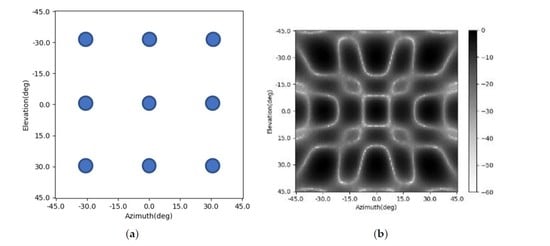
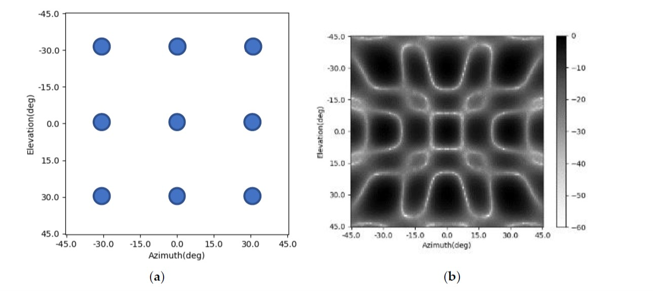
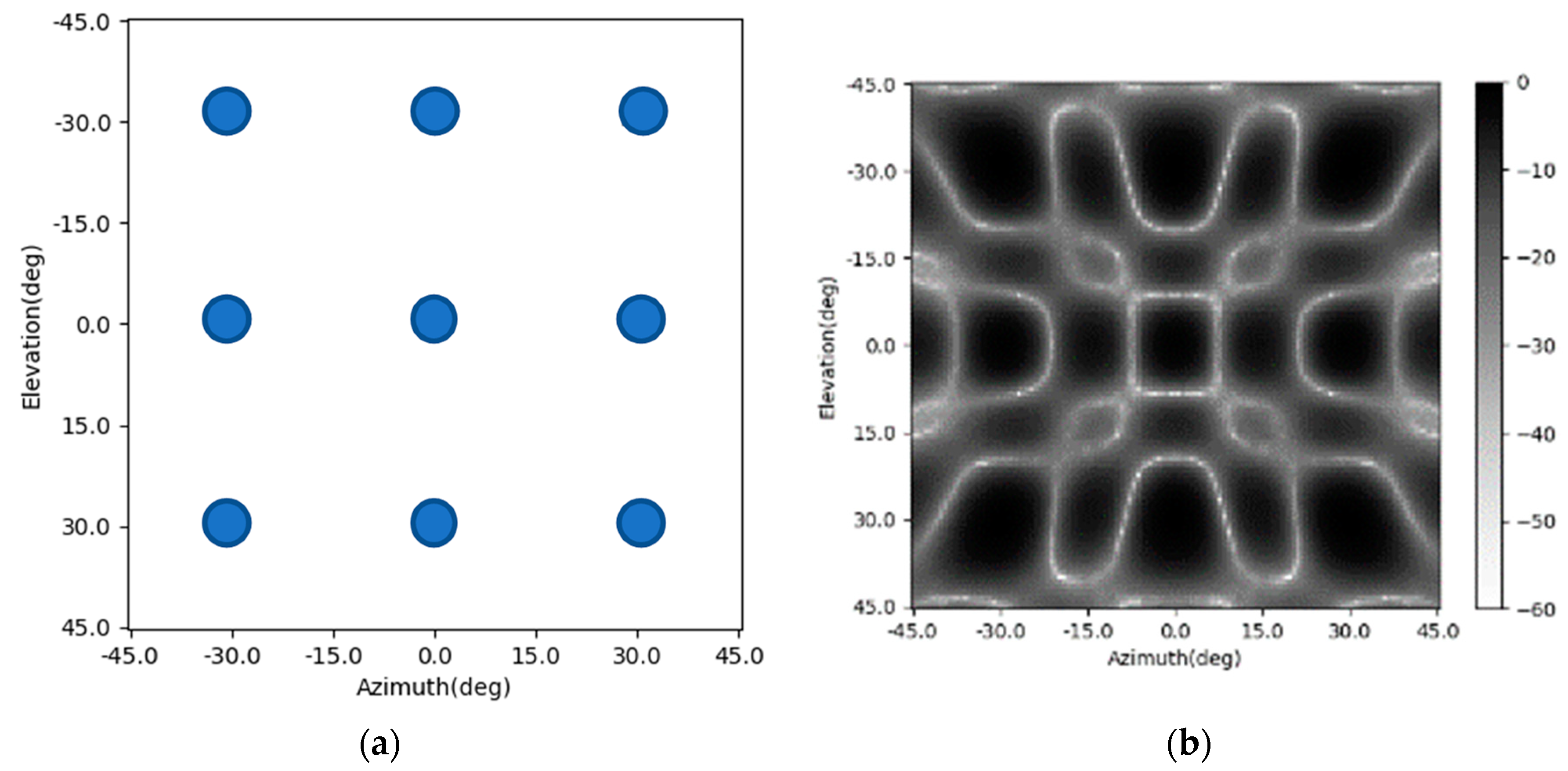
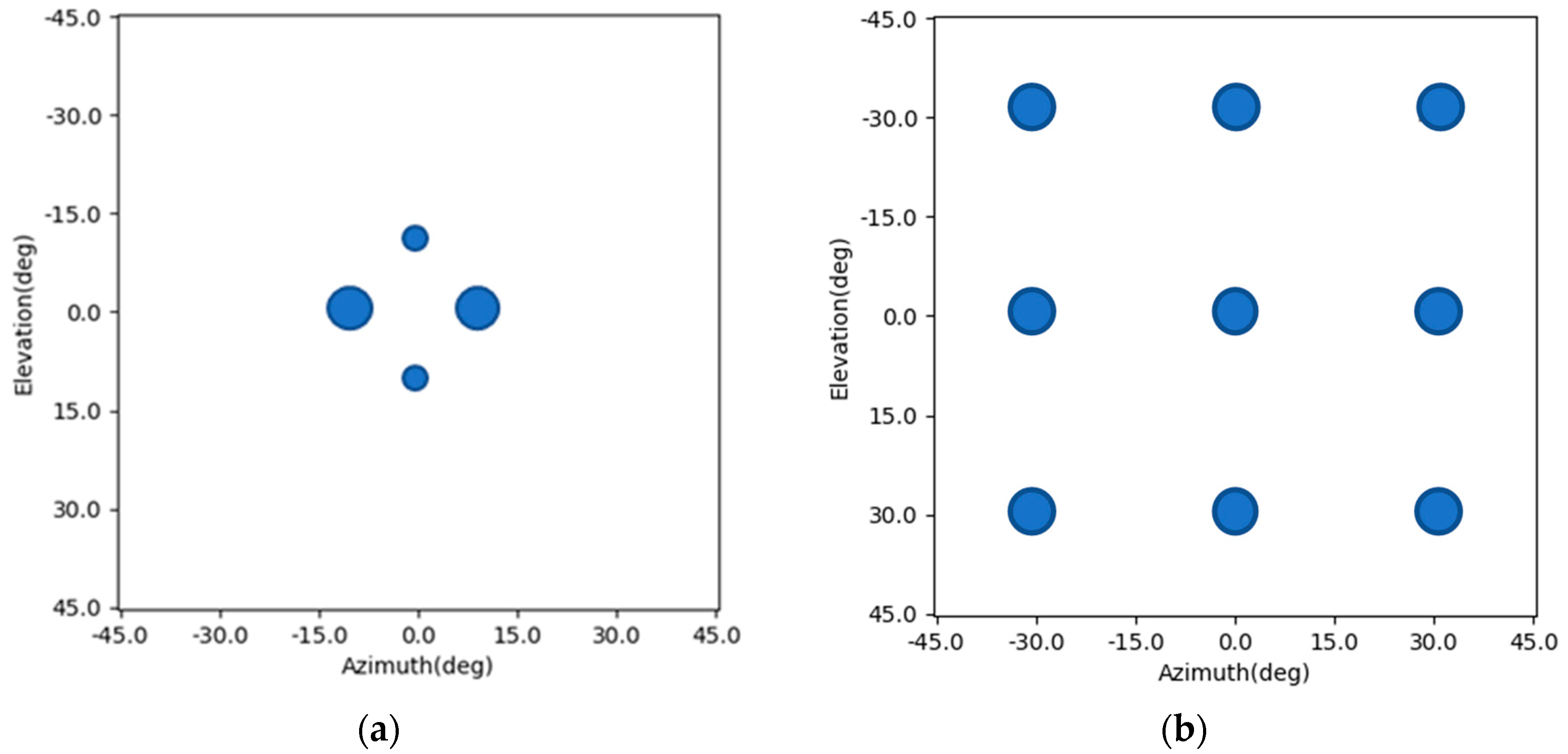
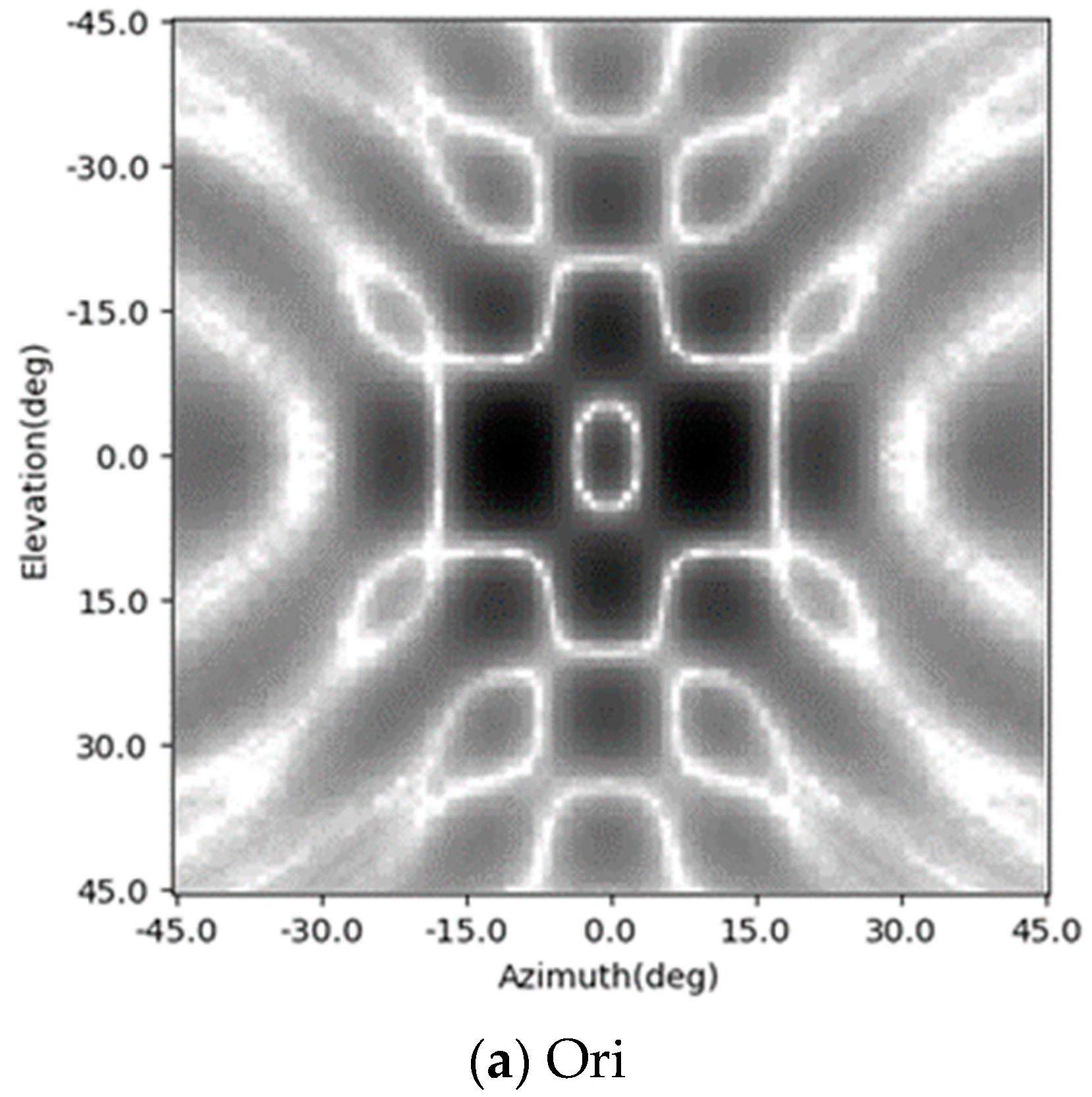
As we can see in (6), there will be cross-terms of and after simplification. So, the shape of the PSF varies with the change of position . Accordingly, the shape of the main lobe in the radar image for a point target depends on its position . It can be illustrated in the following figure. Figure 1a shows an imaging scene with nine point targets. Figure 1b is the corresponding radar image. The shapes of the main lobes of the nine point targets are different due to the difference in their positions.
3. Conventional Radar Image-Enhancing CNN and SV-CNN
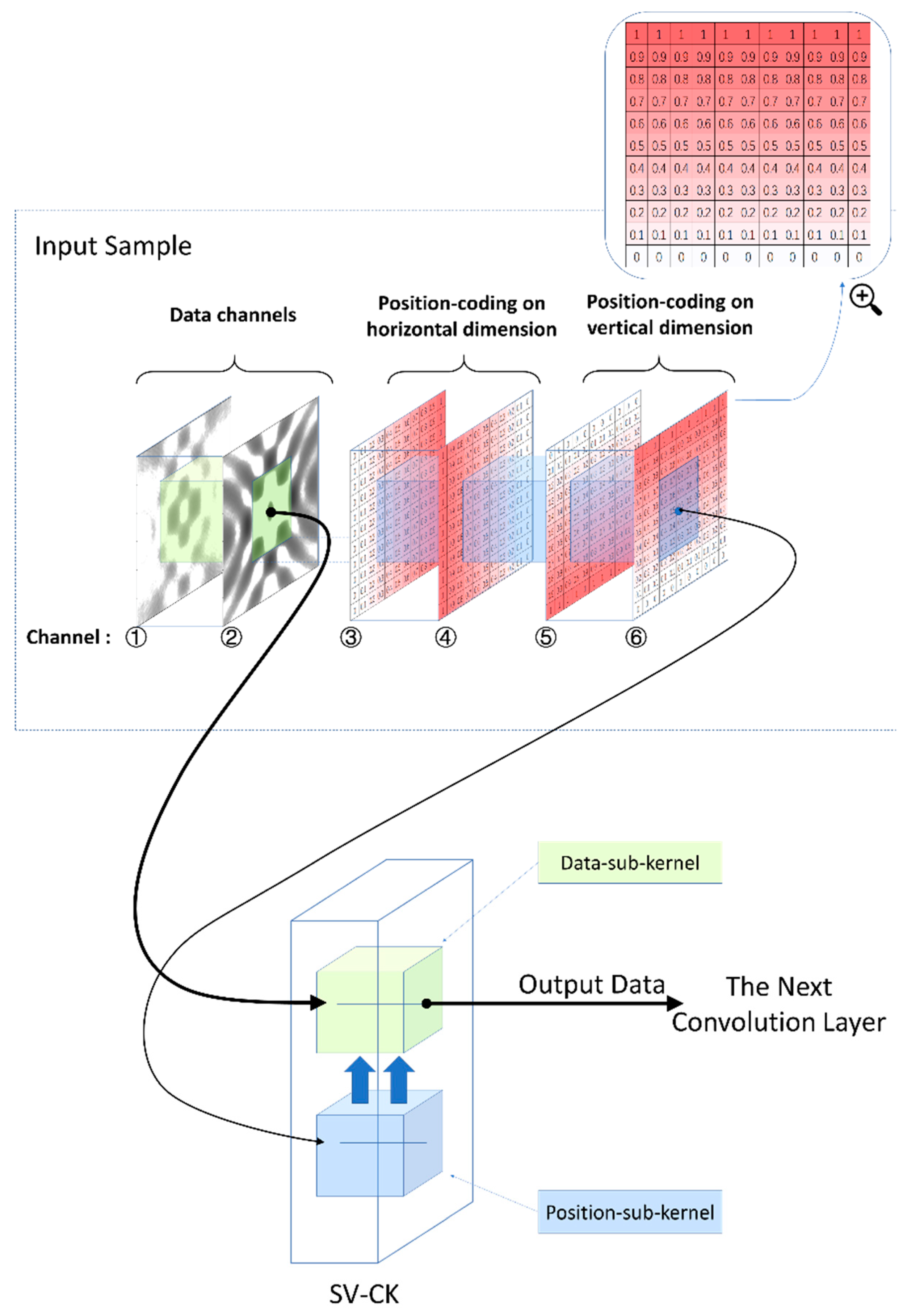
The proposed SV-CK is an evolution of the conventional convolution kernel. The proposed SV-CK contains two parts: a basic data kernel and a position kernel. The position kernel reads information of local position from the position coding embedded into the input sample and controls the data kernel. Thus, the SV-CK has spatial-variant characters.
In this section, the conventional radar image-enhancing CNN in [18] is introduced firstly. Then the SV-CK and SV-CNN are proposed. The enhancing results of the two neural networks are compared in Section 4 to show the advantage of the proposed one.
3.1. Conventional Radar Image-Enhancing CNN
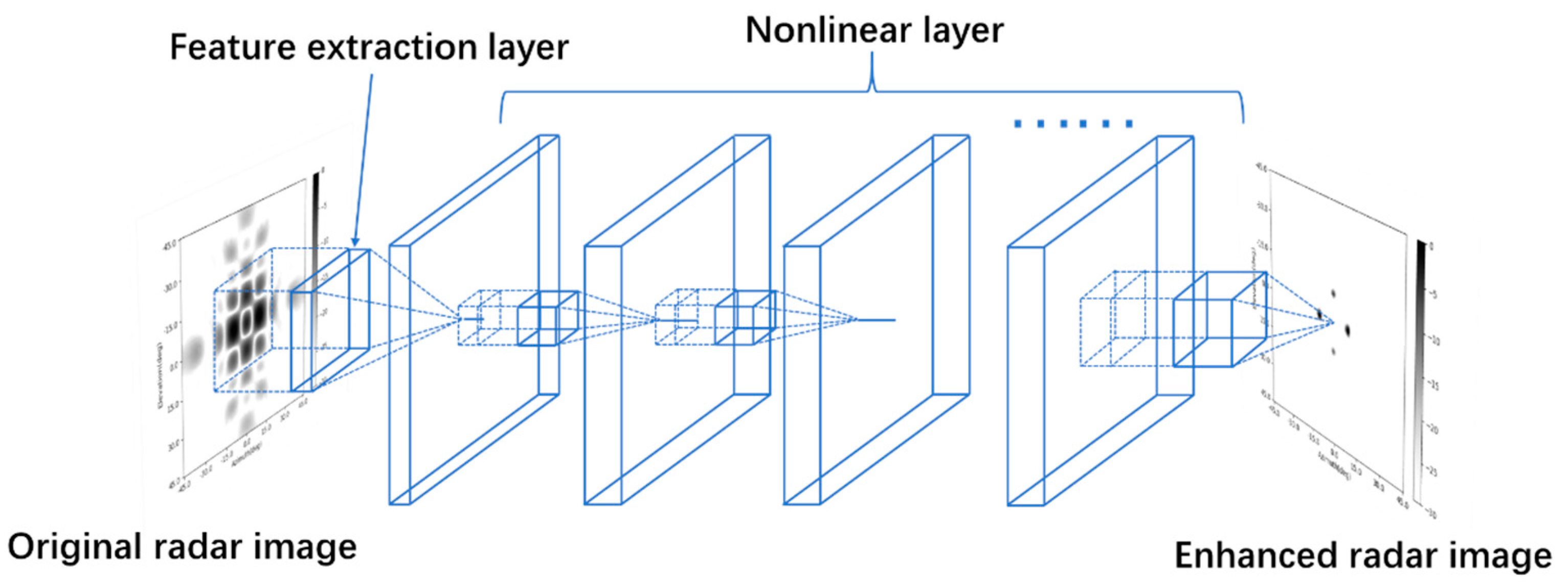
In [18], a convolutional neural network is constructed and trained to enhance the radar image. After enhancement, the main lobes of targets in the radar image are sharpened, and the sidelobes in the radar image are suppressed. Its structure is shown in Figure 2.
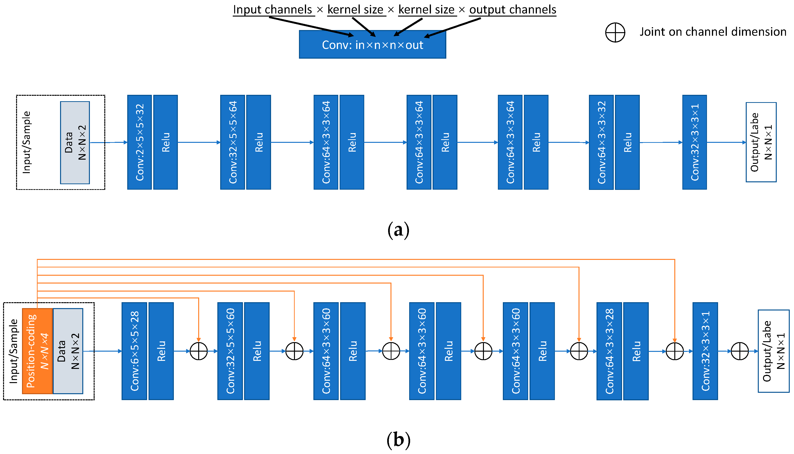
In this paper, a CNN with a similar structure of [18] is constructed to serve as the comparison of the SV-CNN. The CNN is composed of several convolution layers with the rectified linear unit (ReLU) as activation. What is special is that its first layer contains some two-channel convolution kernels. They can take the complex-valued two-dimensional radar image as the input samples (one channel for the real part and the other for the imaginary part). The last convolution layer comprises only one kernel and is not followed by a ReLU. Its output is the final enhanced radar image. The enhancing results can be seen in the next section. The function of this neural network is to sharpen the main lobes and suppress the sidelobes of the radar image. In this way, the radar image is enhanced. However, while enhancing the radar image, the whole CNN can be seen as a spatial-invariant weighted function. The result of each pixel in the enhanced radar image can be seen as the convolution result of the pixels around it and the spatial-invariant weighted function. As discussed earlier, it is more reasonable to use a CNN with spatial-variant convolution kernels to enhance the radar image because of the spatial-variant feature of the motifs in the radar image.
3.2. SV-CK and Position-Coding
As discussed above, a CNN with spatial-variant convolution kernels will give better results when enhancing a MIMO radar image. So, in this section, the SV-CNN is proposed.
The SV-CK and its input sample are shown in the lower half and upper half of Figure 3, respectively. Two parts constitute the SV-CK, which are the data kernel and the position kernel. After being trained, the data kernel reads features from the data channels of the input sample while the position kernel reads the corresponding position information from the position-coding. The position kernel has an influence on the data kernel, and determines what feature it reads and outputs. Thus, an SV-CK is obtained.
The structure of the input samples is shown in the upper half of Figure 3. As discussed before, the first two channels are the input data (complex-valued radar image) and the rest of the four channels are the position-coding. The essences of the position-coding are tensor meshes which indicate the position of each pixel in the data channels. They bring position information into the SV-CNN while training. Consequently, the spatial-variant features can be extracted by the SV-CKs. As shown in the figure, two channels are used to indicate position on one dimension, and the remaining two are used to indicate position on the other dimension. For the two channels of position-coding on the same dimension, the corresponding two elements are complementary, and their sums equal to a constant. Just as shown in Figure 3, the third and fourth channels of the input are the position-coding on the horizontal dimension. The values of the elements on one channel linearly increase, while the values of the elements on the other channel decrease gradually. On the upper right corner of Figure 3, one of the position-coding channels is zoomed in to illustrate its structure more clearly. Specifically, if there is only one channel indicating the position in one direction, the convolution kernels might take it as a constant weighted function of the features, and consequently be confused. The advantage of using two channels of complementary position-coding is indicated in Section 4.
3.3. SV-CNN
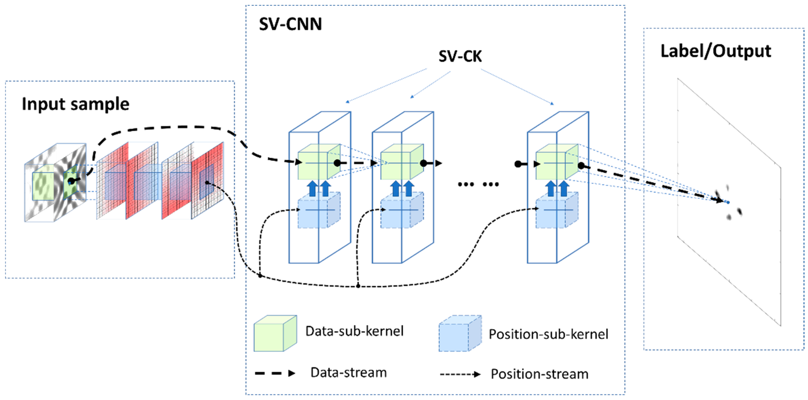
The structure of the SV-CNN is illustrated in Figure 4. There are several convolution layers with SV-CK. The comparison of the CNN and the SV-CNN is shown in Figure 5. During training, the input samples are organized as illustrated in Section 3.2, and the labels are the amplitude of ideal radar image with sharp main lobes and no sidelobe. After being trained, the network takes complex-valued radar images with four-channel position-coding as the input and outputs amplitude of enhanced radar images with sharp main lobes and low sidelobes.
As shown in Figure 4 and Figure 5b, there are two streams in the SV-CNN. (1) The first one is the data stream. The data kernel extracts the features from the input sample or the output of the former layer and outputs feature maps to the next layer until the final output (the enhanced radar image) is obtained. (2) The second one is the position-coding stream. Position-codings are transmitted to position kernels in each layer through skip connection. It helps the position kernels to read the information of the local position and guides them to control the corresponding data kernel. The input data are covered by four channels of position-codings. The convolution kernels process the data and the position-coding together, and the ReLU after each of the convolutional layers will totally mix them up. The parameters which determine the relationships between the position-codings and the data are contained in the convolution kernels and can be optimized through training. Thus, an SV-CNN is obtained and its superiority is tested in the next section.
4. Implementation and Simulation
In this section, some features of the SV-CNN are tested. Firstly, in part A, the training procedure of the SV-CNN and its enhancing results are given. Then, in part B, the training loss and the testing loss of the SV-CNN are compared to those of a CNN with a similar structure to show the superiority of the SV-CNN. In part C, the guided backpropagation method is used to discover the influential information in the input samples. The results showed that the position-coding does offer useful information for the SV-CNN. Finally, in part D, the guided backpropagation method is used to show the importance of position-coding on each layer. Then, the position-codings which make no difference to the final result are cut off to reduce the complexity of the SV-CNN.
4.1. Structure of the SV-CNN and the Training Procedure
A seven-layer SV-CNN was proposed to enhance the radar image. An illustration of the structure is shown in Figure 4 and its specific structure and the compared CNN are shown in Figure 5. The input samples are organized as illustrated in Section 3.2. There are two channels for data and four channels for the position-coding. The four position-coding channels are inset into the input of each layer through the skip connection as illustrated in Figure 4 and Figure 5b.
The samples and the labels are valued while training the neural network. While generating the samples, three steps are taken. Firstly, simulate several point scatterers in the imaging scene. Then, simulate the radar signal and the corresponding echo of these point scatterers. Finally, calculate the original radar images as the input samples. As for the labels, just project the RCS of each simulated point on the RCS distribution maps whose value of each pixel equals to the RCS of the point target at the corresponding position. If the pixel does not correspond to a point scatterer, then its value is zero. A total of 22,000 sample label pairs like this were simulated; 20,000 of them were randomly chosen to train the neural network and 2000 of them were chosen to test it.
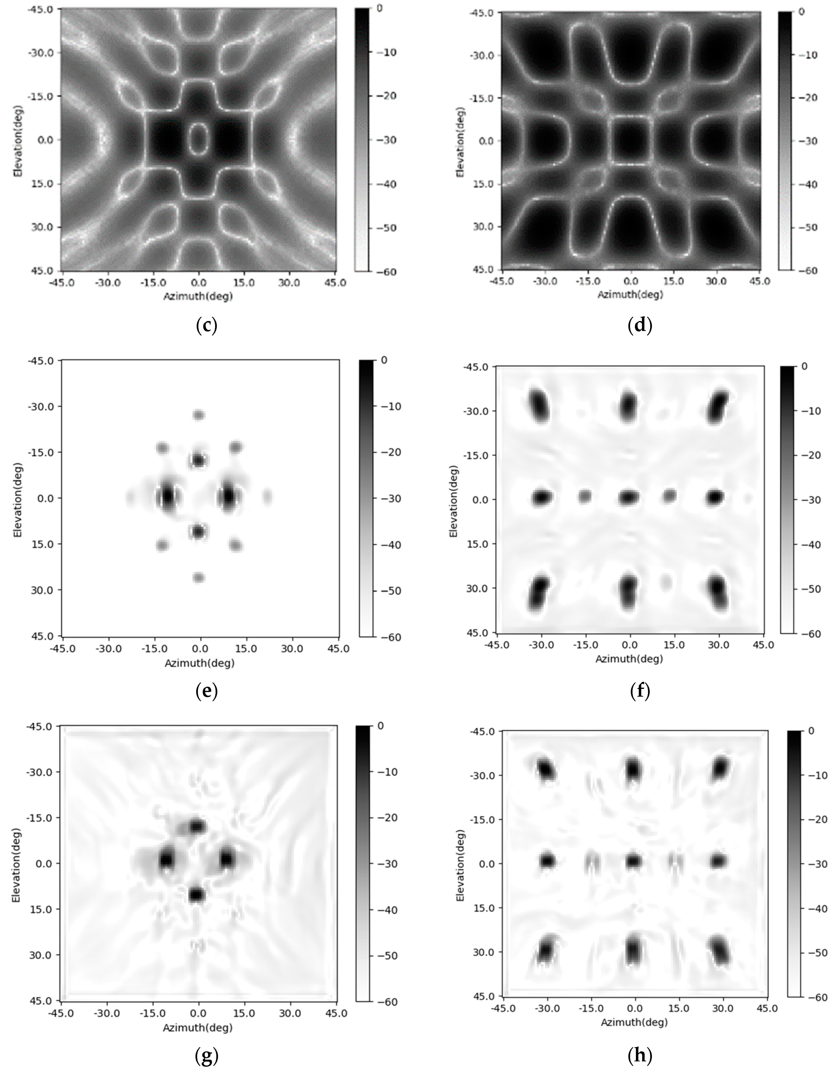
The training procedure is evaluated on a PC with a CPU of I7, two pieces of 16 GB RAM, and a GPU of 2080 Ti. The networks are established using the PyTorch. After being trained, the SV-CNN is given the ability to enhance the radar image. The original radar images and the enhanced ones are shown in Figure 6. Besides, the enhancing results of the SV-CNN are compared to the enhancing result of the CNN trained using the same procedure. The structure of the compared CNN is illustrated in Figure 5a. Two imaging scenes were simulated as shown in Figure 6a,b. The original radar images are shown in Figure 6c,d. The enhancing results of the CNN are shown in Figure 6e,f, and the enhancing results of the SV-CNN are shown in Figure 6g,h. As we can see in the figure, after enhanced, the main lobes of motifs in the radar image are sharpened and the sidelobes are suppressed. However, there are false peaks in the enhancing result of the CNN. The false peaks might result in false alarms in the detection procedure, which is unacceptable. So, the SV-CNN performs better while enhancing radar images. The detailed performance of the networks is summarized in Table 1.
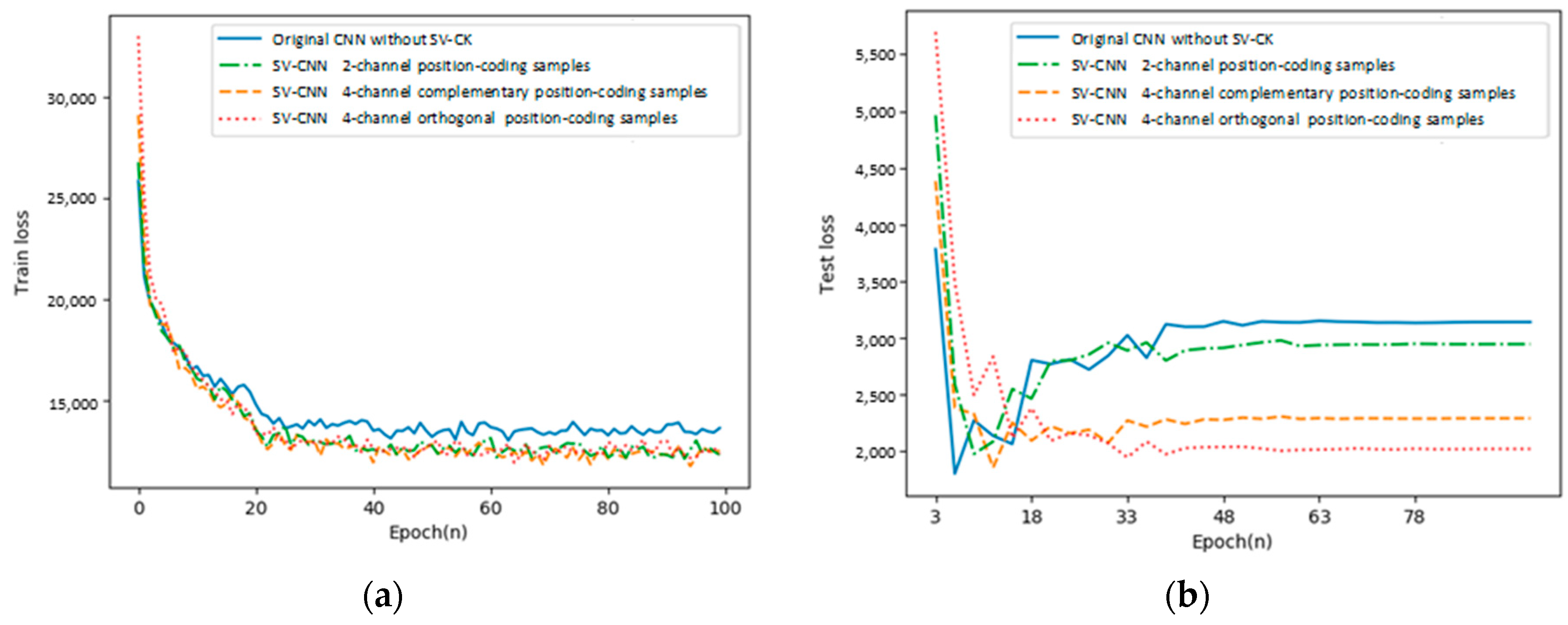
4.2. Comparison of CNN and SV-CNNs Trained Using Samples with Different Forms of Position-Coding
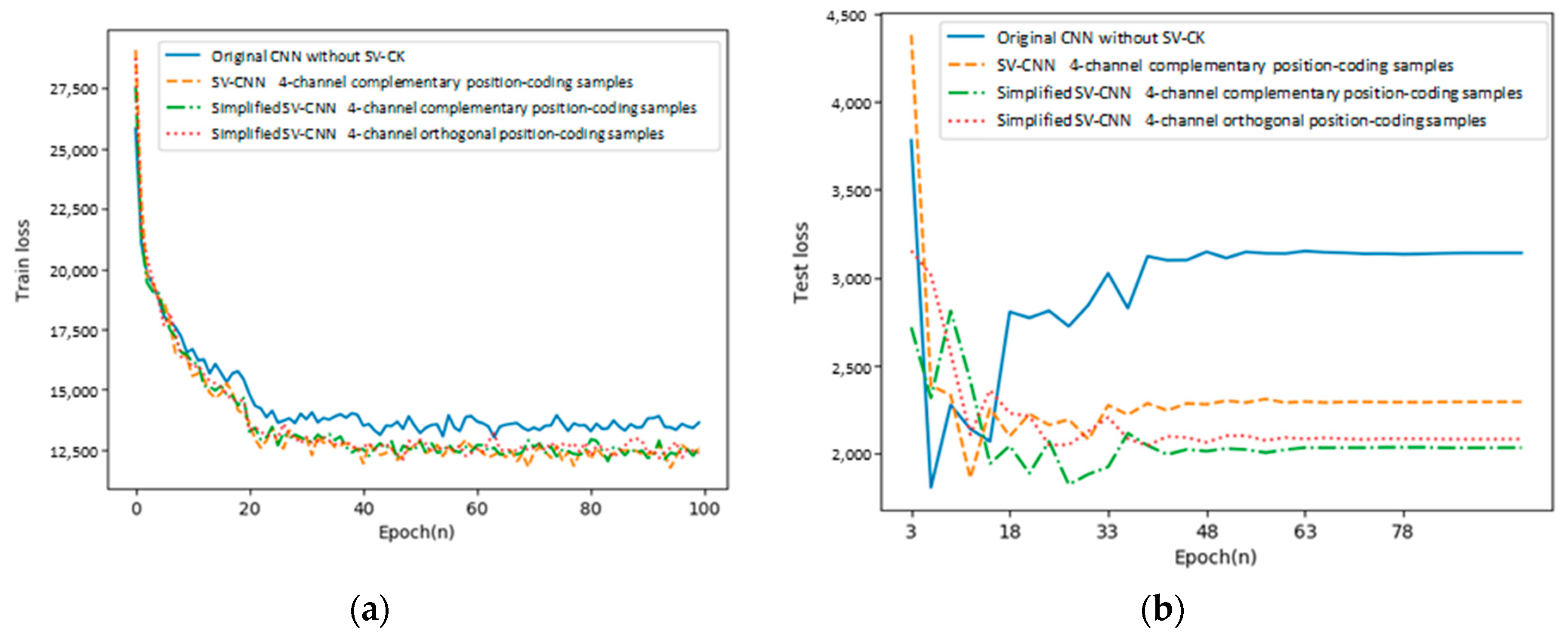
In this part, the training loss and the testing loss of the proposed SV-CNN are compared to the other three networks. (1) The conventional CNN; (2) the SV-CNN trained using samples with two position-coding channels. Its input samples are with the similar structure shown in Figure 3, however, only the third and the fifth channels serve as the position-coding, and each channel indicates the position on one direction; the fourth and the sixth channels are deleted. (3) SV-CNN trained using samples with four orthogonal position-coding channels. The four complementary position-coding channels are processed by the sinusoidal function, and then they became orthogonal to each other, while training with the same parameters. The training loss and the testing loss of these CNNs are shown in Figure 7a,b, respectively.
As shown in the figure, both the training loss and the testing loss of the SV-CNN trained using samples with four position-coding channels (both complementary and orthogonal) decrease the fastest, and after the networks stabilize, both the training loss and the testing loss of the SV-CNN trained using samples with four position-coding channels are lower.
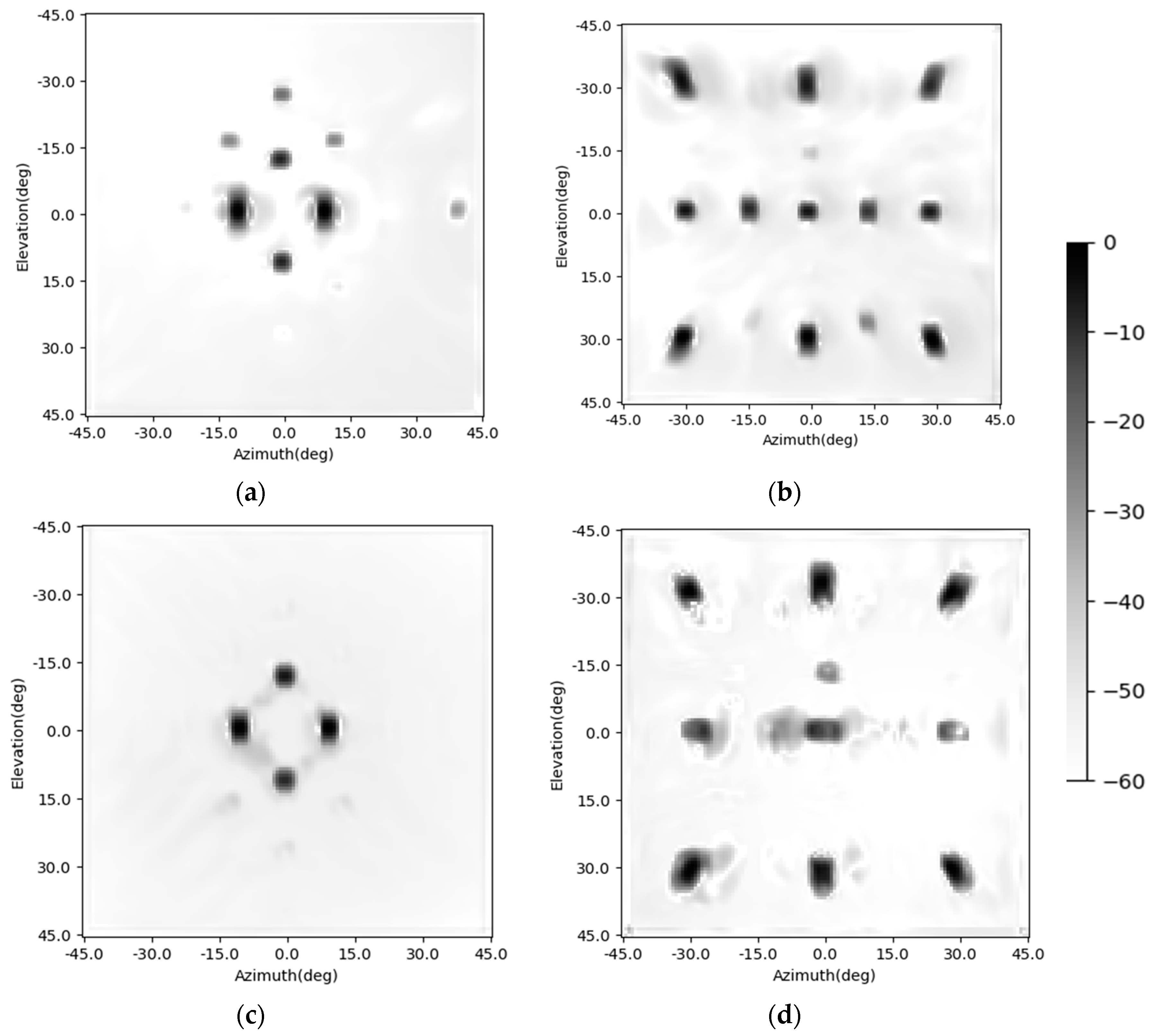
Besides, the enhancing results of the four CNNs are shown in Figure 6 and Figure 8. The imaging scenes are set as Figure 6a,b. Their corresponding imaging results are shown in Figure 6c,d. The enhancing results of the CNN are shown in Figure 6e,f. The enhancing results of the SV-CNN trained using samples with four complementary position-coding channels are shown in Figure 6g,h. The enhancing results of the SV-CNN trained using samples with two position-coding channels are shown in Figure 8a,b, and those of the SV-CNN trained using four orthogonal position-coding channels are shown in Figure 8c,d. The dynamic ranges of all these figures are assigned as 60 dB. As shown in the figures, the false peaks occur in the enhancing results of the conventional CNN and the SV-CNN trained using samples with two position-coding channels. What is even worse is that the enhancing results of the SV-CNN trained using samples with two position-coding channels become asymmetric due to the asymmetric position-coding values. Both the SV-CNNs trained using samples with four position-coding channels have better effects on suppressing the sidelobes.
4.3. Testing the Function of SV-CK and Position-Coding
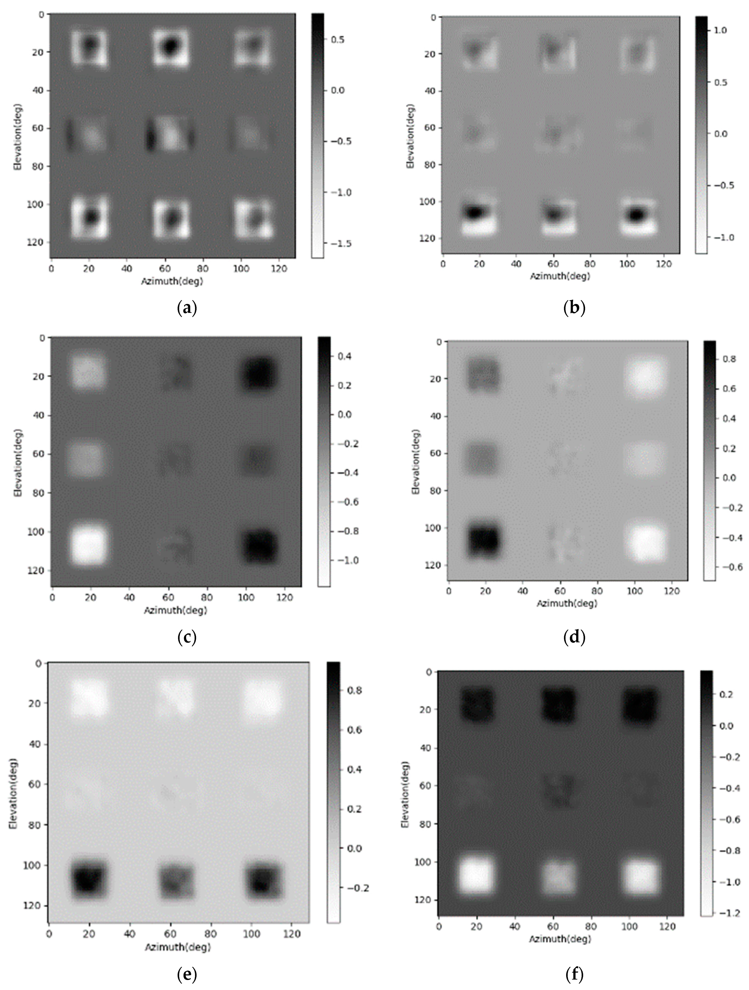
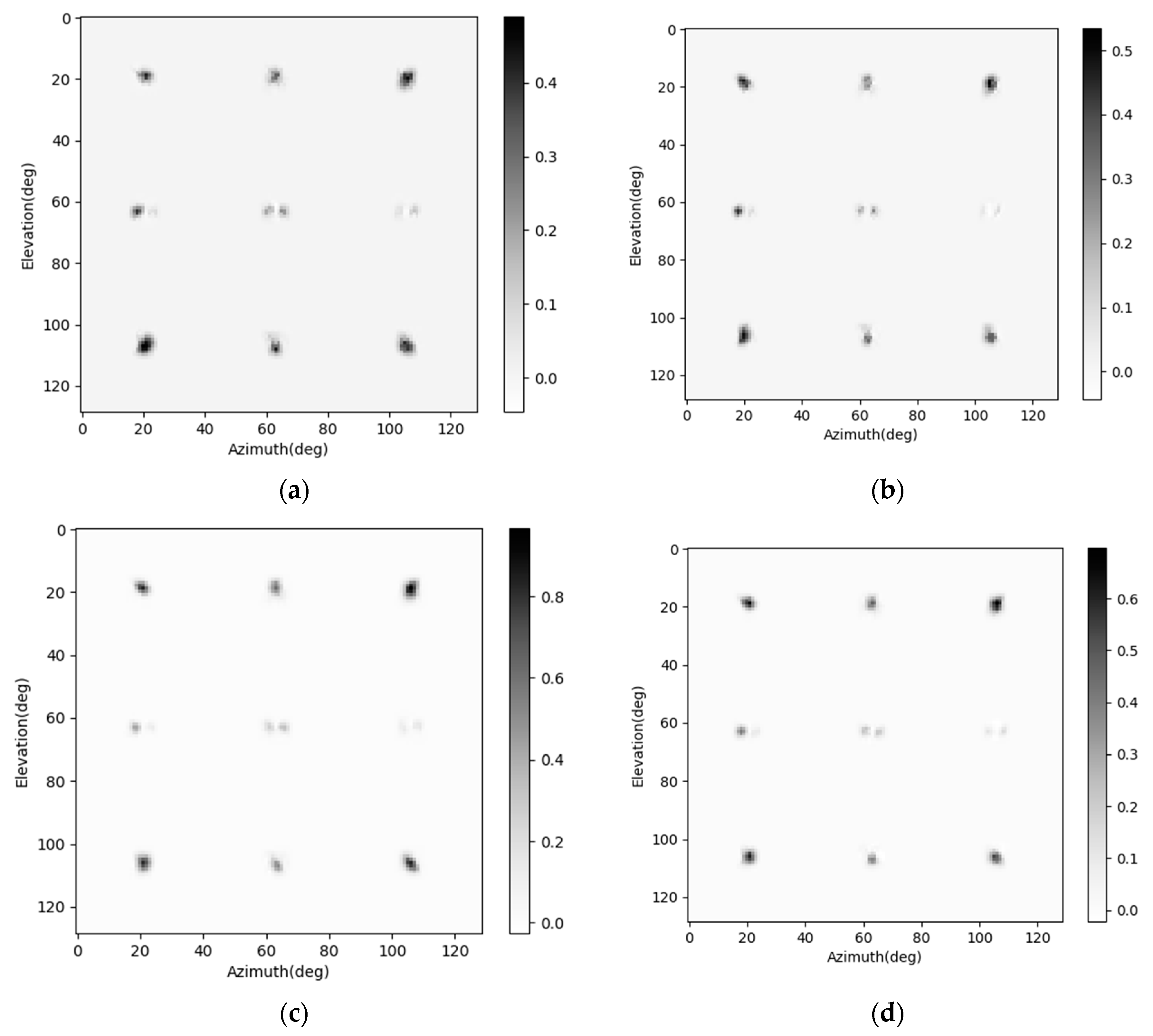
In this part, the guided backpropagation method is used on the SV-CNN to show if the SV-CKs extract local position information from the position-coding. The guided backpropagation is a combination of the deconvolution method and the backpropagation method [29,30,31]. It is an efficient way of visualizing what concepts in the graph have been learned by the neural network. An imaging scene shown as Figure 6b is simulated. There are nine point targets in the simulated imaging scene, and the corresponding radar image is as shown in Figure 6d. The guided backpropagation method is used to show what concepts the network took while enhancing this sample. The influential concepts on each channel of this sample are shown in Figure 8. The results on two data channels are shown in Figure 9a,b. The reception field and important features that the network used to enhance the radar image can be seen in these figures. The guided backpropagation results on the four position-coding channels are shown in Figure 9c–f. The influential features on the horizontal dimension are shown in Figure 9c,d, and the influential features on the vertical dimension are shown in Figure 9e,f. As shown in these figures, the tendency of values read from the two complementary position-codings on the same dimension is contrary. This tendency is in accord with the tendency of the position-codings. This phenomenon confirms that the position information contained in the position-coding is extracted by the network.
4.4. Simplification of the SV-CNN
As shown in Figure 4 and Figure 5b, the four position-coding channels are inset into the input of each layer through the skip connection. These skip connections increase the complexity of the SV-CNN. In this part, the guided backpropagation method is used to evaluate the weightiness of the position-codings inset into each layer, and cut off the unnecessary ones. The guided backpropagation method is used to show what the SV-CNN extracts from the input of each layer. If there is no obvious spatial-variant feature extracted from the position-codings of one layer, then they are not necessary.
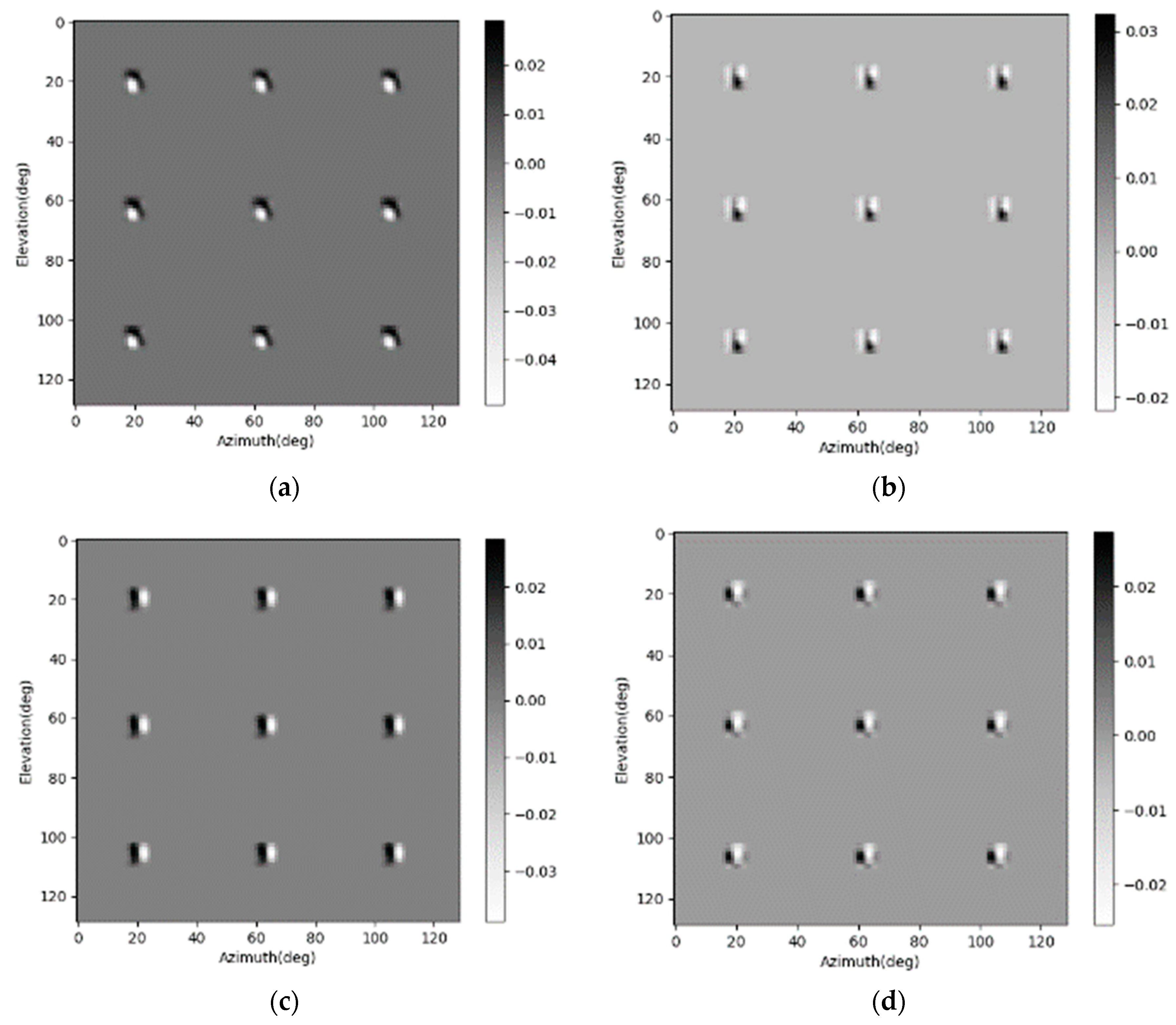
The guided backpropagation results on the position-codings of each layer are calculated, and those of the first, the sixth, and the seventh layers are shown in Figure 9, Figure 10 and Figure 11, respectively. As we can see, for the simulated nine point scatterers, the guided backpropagation results on the position-codings of the first layer vary tremendously. The backpropagation results on the position-codings of the sixth layer only vary slightly. As for the seventh layer, the backpropagation results have hardly any variety. The results mean that, for the first and the sixth layer, the spatial-variant features in the input data are extracted by the SV-CK, while the SV-CKs in the seventh layer do not extract these spatial-variant features. Thus, the corresponding skip connection from the position-codings to the seventh layer is unnecessary and can be cut off. In this way, the SV-CNN is simplified. Then, using the same training method in Section 3.1 to train the network, the training loss and testing loss of the simplified SV-CNN are shown and compared in Figure 12. As we can see in the figure, after simplification, there is no significant degradation on both the training loss and the testing loss. Besides, after simplification, its training loss and testing loss are still lower than those of the conventional CNN, and they may sometimes be even lower than those of the SV-CNN that has not been simplified.
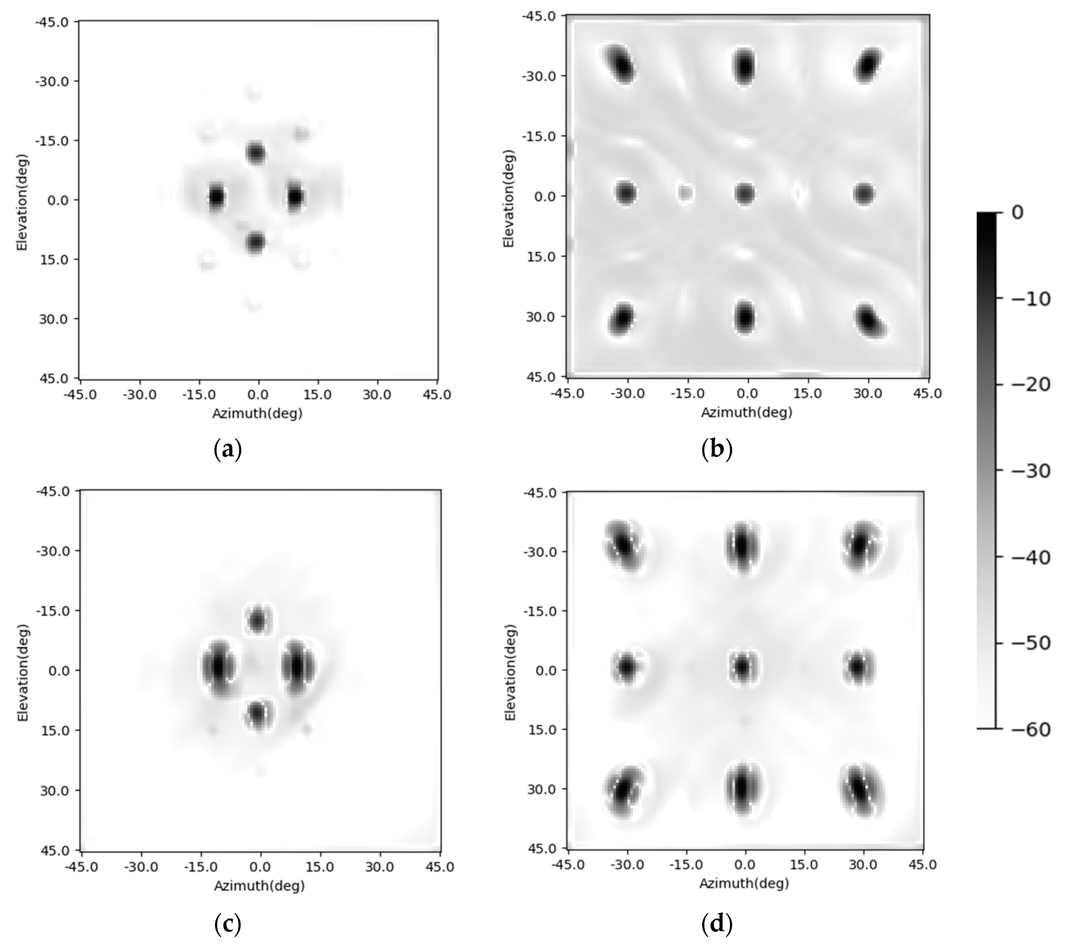
The enhancing results of the simplified SV-CNN are shown in Figure 13. The imaging scene is the same as those illustrated in Figure 6. The upper row is the enhancing result of the simplified SV-CNN trained using samples with four complementary position-coding channels, while the lower row is the enhancing result of the simplified SV-CNN trained using samples with four orthogonal position-coding channels. The dynamic ranges of all the figures are set to 60 dB. Compared to the enhancing results shown in Figure 6 and Figure 7, there is no obvious degradation in the performance of the simplified SV-CNN. The performance of the simplified SV-CNN is still higher than that of the CNN. Besides, the simplified SV-CNN trained using samples with four orthogonal position-coding channels sometimes performs better in sidelobe suppression (Figure 13d).
The SV-CNNs are trained and analyzed in this simulation part. It can be seen from the simulation results that compared to the CNN and the SV-CNN trained using samples with two position-coding channels, the SV-CNN trained using samples with four position-coding channels performs better in enhancing radar images. The SV-CNN trained using samples with both four complementary position-coding channels and four orthogonal position-coding channels has good performance in enhancing radar images. Besides, the performance of the simplified SV-CNN does not degrade obviously, and is sometimes even better. The maximum sidelobe levels (MSLLs) of the enhancing results of the above networks are listed in Table 1. The results also support the conclusion that the networks with four channels of position-codings perform better. For the original radar images, there is more than one point target in both of the images. So, their sidelobes are accumulated and higher than the theoretical value of −13.2 dB.
4.5. Comparison to Other Existing Methods
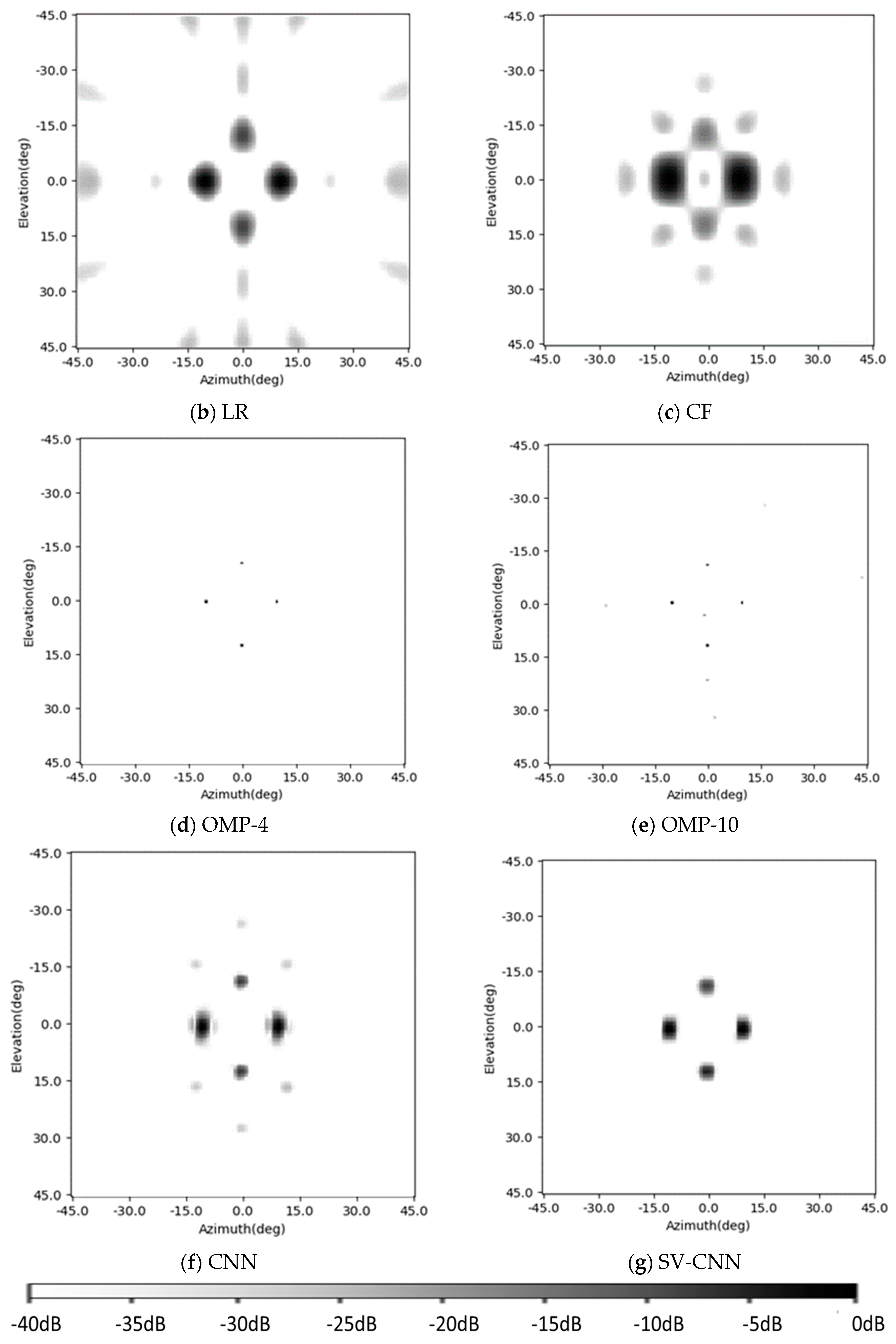
In this part, the enhancing results of the four-target scene in Section 4.1 are reviewed, and another three existing methods are added into the comparison. This time, the Gaussian noise is added to the simulated signal and makes the signal-to-noise ratio 15 dB. The original radar image, the enhancing results of the CF algorithm [23,24,32,33], the results of the orthogonal matching pursuit (OMP) sparsity driven method [27], and the Lucy–Richardson deconvolution algorithm [28] are shown in Figure 14a–e, respectively, and the results of the CNN and the SV-CNN are shown in Figure 14f,g, respectively. Besides, the MSLLs of these methods are listed in Table 2.
It can be seen from the results that all of these methods can suppress the sidelobes and improve the quality of the images. In the original, the sidelobes of these four points overlap, and this makes the MSLL higher than the test theoretical value of −13.2 dB. The Lucy–Richardson deconvolution and the CF algorithm can suppress the sidelobes to −28.39 dB and −27.75 dB, respectively. The performance of the OMP algorithm strongly depends on the parameter of the sparsity. If it is set as 4 and equals the number of the targets, there will be no sidelobes. However, in real-world detection, it cannot be foreseen. So, a result of the OMP with the sparsity of 10 is also given. With the interference of noise, there are sidelobes with MSLL of −22.85 dB. In the results of the CNN and the SV-CNN, the MSLL is −25.11 dB and −42.71 dB, respectively. According to the above results, the SV-CNN offers better results, especially when compared to the conventional CNN.
5. Experiment
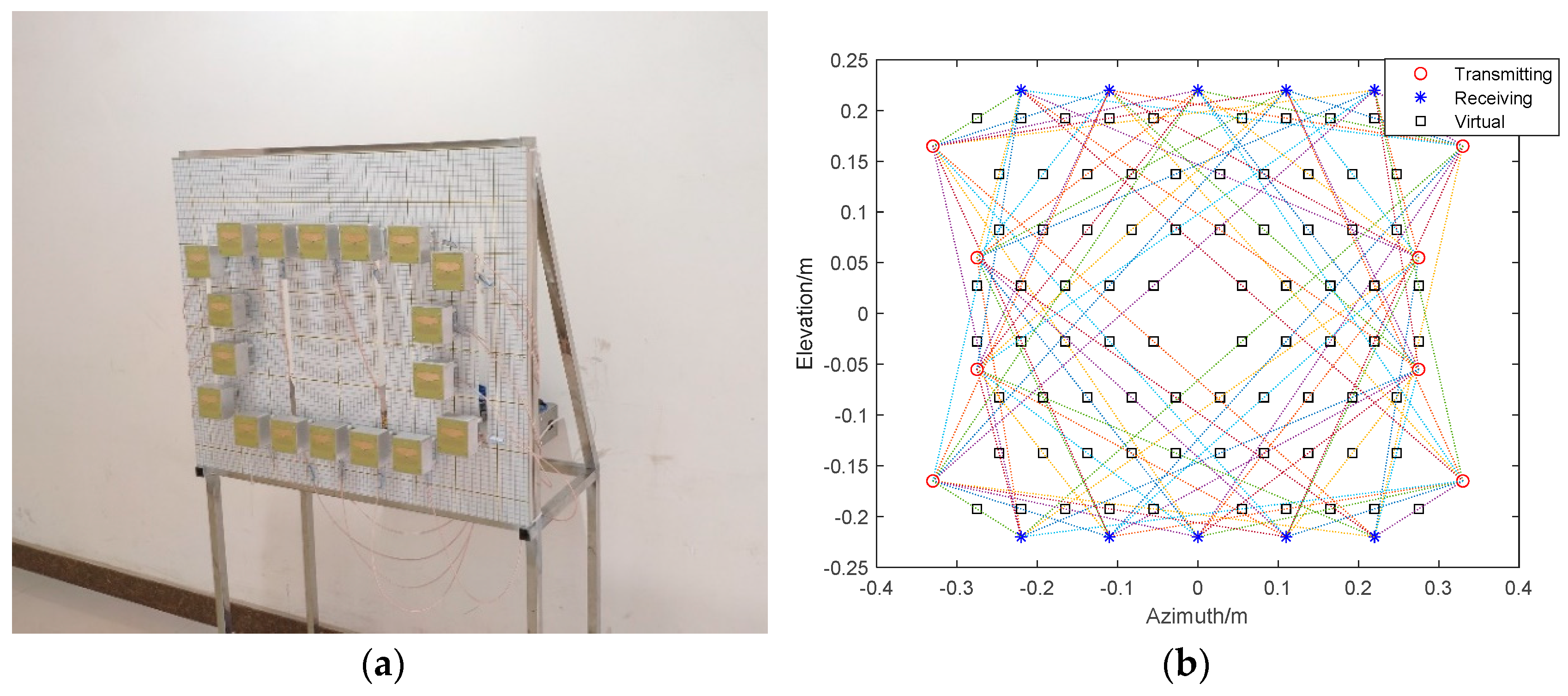
In this experiment part, a radar device is implemented to obtain the radar image of the imaging scene and test the proposed SV-CNN. The MIMO radar is shown in Figure 15. The small units fixed on the plane are its antenna. Eight of them are transmitting antennas and 10 of them are receiving antennas. During operation, the transmitting antennas take turns to transmit L/S band signal with 600 MHz bandwidth, and the receiving antennas take turns to receive the echo signal. It takes 0.1 s to switch all the antenna channels. Then, the radar images of the imaging scene can be obtained through the BP algorithm illustrated in Section 2.
5.1. Performance for Point Targets
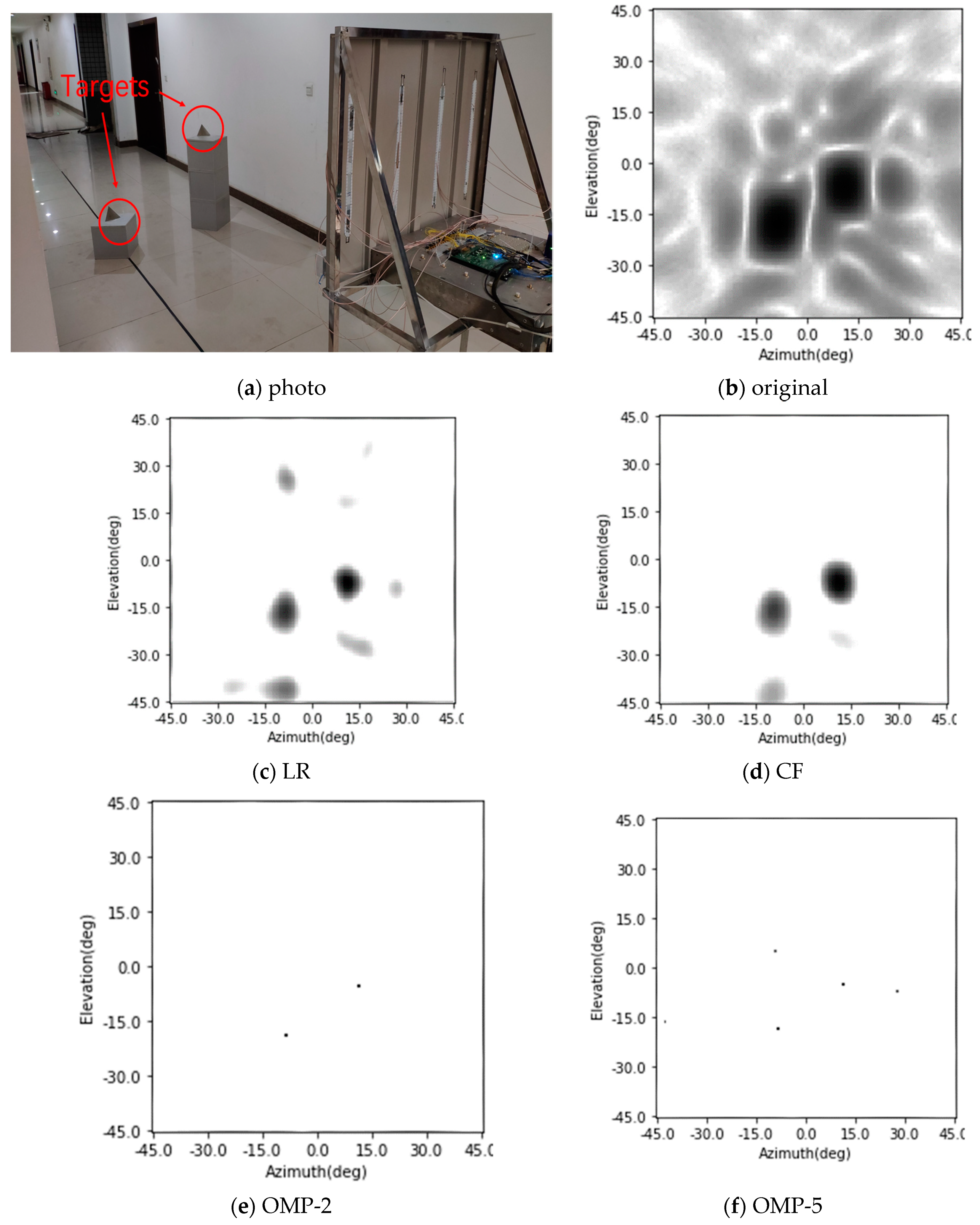
In this part, the imaging and enhancing results of two corner reflectors are given. The imaging scene in this experiment is shown in Figure 16a. Two corner reflectors are placed in front of the radar system. The point scatterers are 3 m away from the center of the radar antenna array. The original radar image of the imaging scene is shown in Figure 16b, and the enhancing results of the Lucy–Richardson deconvolution and the CF algorithm are shown in Figure 16c,d, respectively. The enhancing results of the OMP with the sparsity of 2 and 5 are shown in Figure 16e,f, respectively. Finally, the enhancing results of the conventional CNN and the simplified SV-CNN trained using samples with four position-coding channels are shown in Figure 16g,h, respectively. The MSLLs of these results are listed in Table 3.
It can be seen in the results that the sidelobes in the real recorded radar image are a little higher than in the simulation one, because the scatterers used are slightly expanded ones. Compared to the simulation results, the performance of the Lucy–Richardson deconvolution slightly degrades, because of these expanding characters. The results of the OMP with the sparsity of 2 is still free of sidelobes. However, the performance of the OMP with the sparsity of 5 degrades because of the inevitable noise and the mismatch between the real system and the theoretical model. From the results, we can see that the SV-CNN also offers the best results in our occasion.
5.2. Performance for Extending Targets
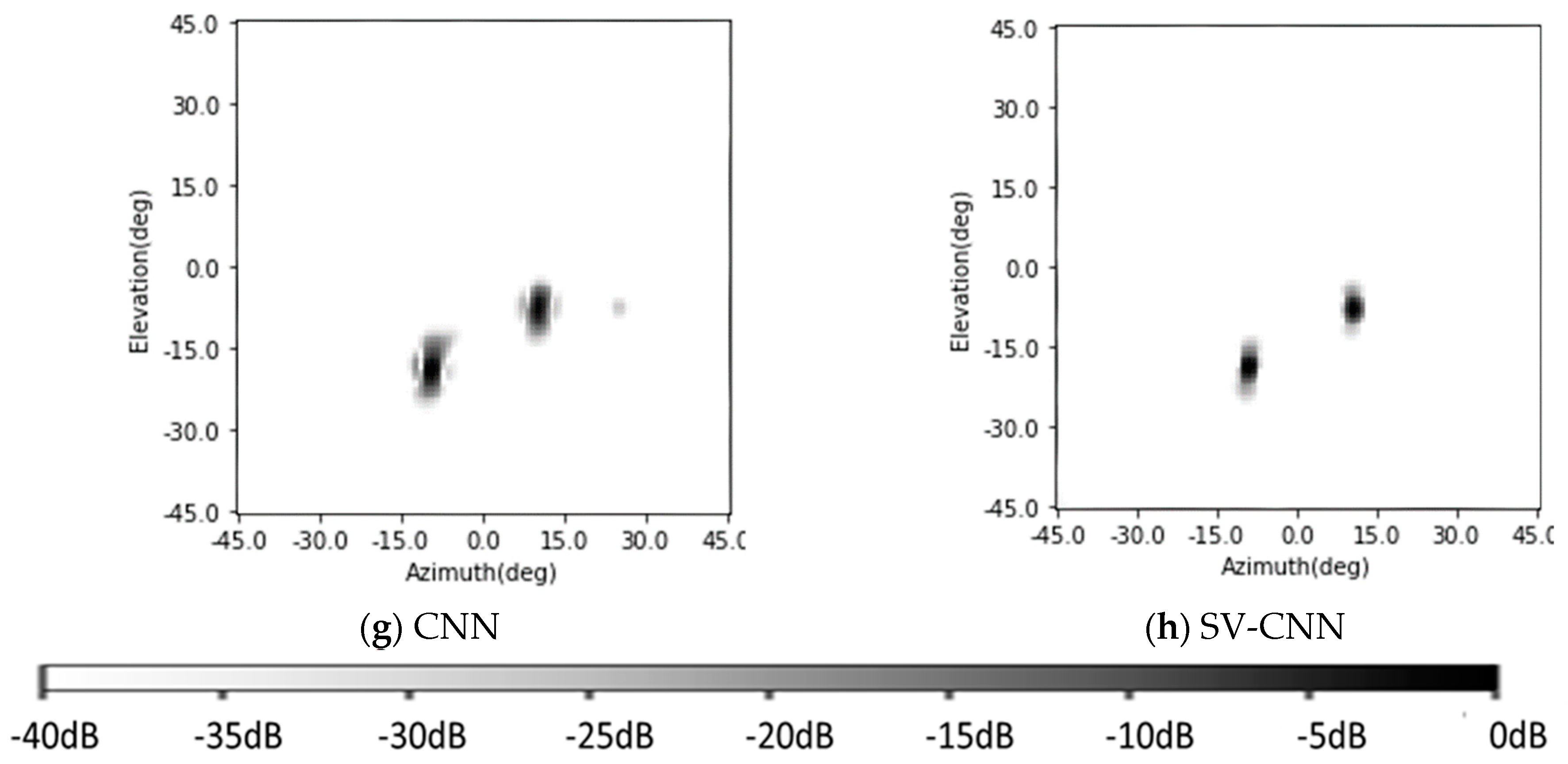
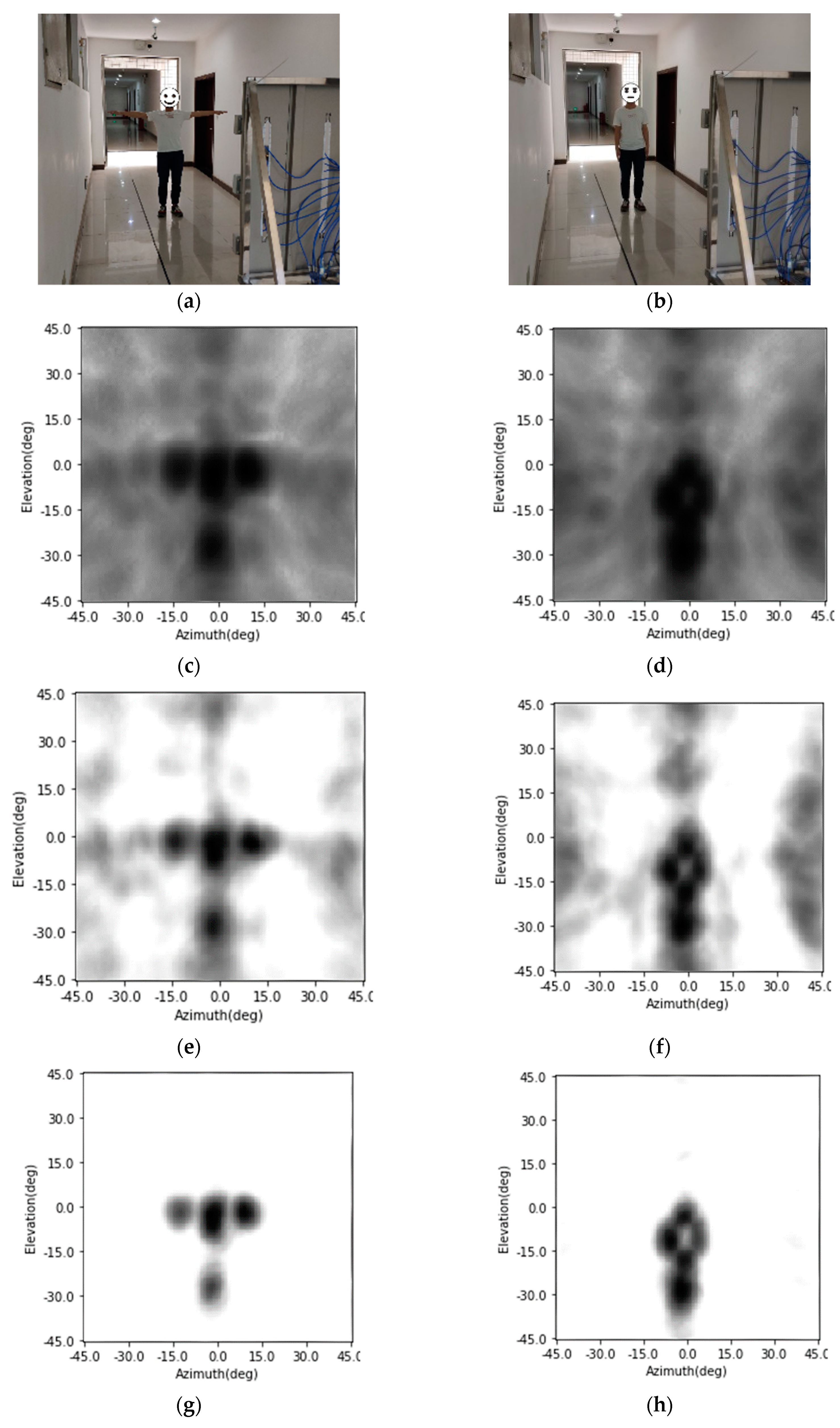
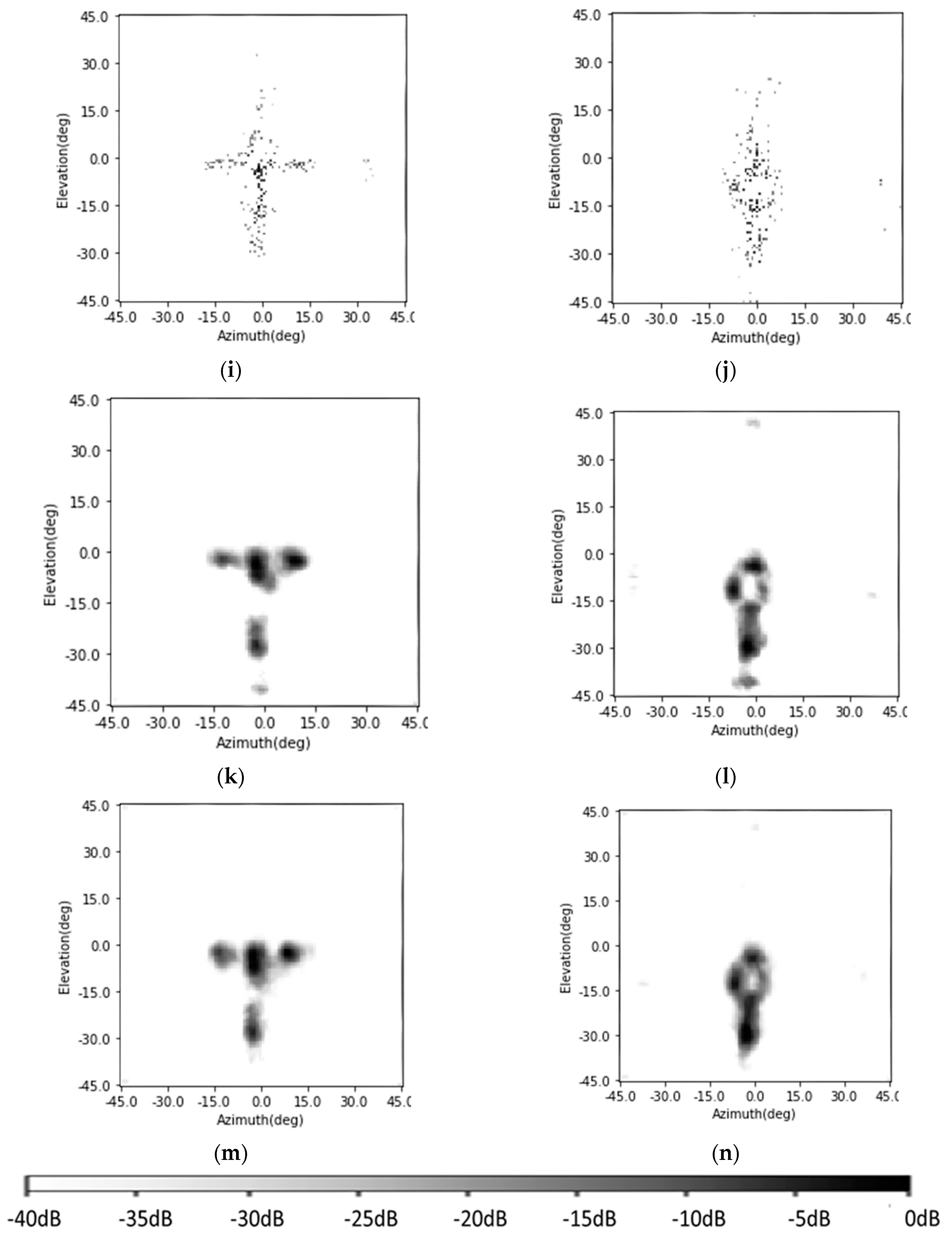
In this part, the SV-CNN is used to enhance the radar images of human targets to evaluate the degradation in a real setup. The radar images of a human body are enhanced using the SV-CNN. The photo of the imaging scene is as shown in Figure 17a,b. A human stands 3 m away from the radar and with his arms opening and dropping, respectively. The original radar images are shown in Figure 17c,d, respectively. The enhancing results of the Lucy–Richardson deconvolution algorithm, the CF algorithm, the OMP algorithm, the CNN, and the SV-CNN are shown in Figure 17. The power reflected by the human limbs varies strongly with the variety of the incident angle of the radar signal. So, the final enhanced radar image is obtained through accumulating the enhancing results of several continuous frames of images. Because of the accumulation, the quality of all these images is improved. As can be seen, for these extremely extended targets, the sidelobes of the Lucy–Richardson is the highest for it is originally proposed for real-valued optical images. The results of the OMP are faced with several sidelobes when dealing with the real recorded targets, as well as the CNN (at about (0°, −42°)). The sidelobes in both results of the CF and the SV-CNN are low. However, the proposed SV-CNN offers sharper main lobes. In all of these enhanced results, the actions can be easily discriminated. However, the SV-CNN offers the best results.
6. Discussions
In this paper, we proposed the SV-CNN to deal with images with spatially variant features. Compared to conventional CNN, the proposed SV-CNN is with spatial awareness. Thus, the SV-CNN performs better when faced with spatially variant features.
In Section 4 and Section 5, we use the proposed SV-CNN to suppress the sidelobes in MIMO radar images as an illustration. The enhancing results of the proposed SV-CNN are compared to several state-of-art methods including the CF algorithm [23,24,32,33], the OMP sparsity driven method [27], and the Lucy–Richardson deconvolution algorithm [28], as well as the conventional CNN.
Since the MIMO radar images in our condition are with spatially variant features (as illustrated in Figure 1), our proposed SV-CNN performs best among these methods. The superiority of the SV-CNN can be seen in Figure 14, Figure 16 and Figure 17.
Besides, it is pointed out that the SV-CNN should extract spatial information from four-channel position-codings. The enhancing results will degrade and even become asymmetric when there are only two channels of position-coding, because the network might take the two channels of position-coding as a weight function to show the degree of importance of the input samples. Simulation results in Section 4.2 support this standpoint.
7. Conclusions
In this paper, a spatial-variant convolutional neural network (SV-CNN) with spatial-variant convolution kernels (SV-CK) is proposed. While extracting features, the proposed SV-CNN can take the local position information into account compared to conventional CNNs. Thus it has better performance when the shapes of the motifs in the images depend on the local position.
The proposed SV-CNN is trained to enhance the radar images to illustrate its function. After being trained using radar images with position-codings, it can suppress the sidelobes in the radar images. The SV-CKs can extract spatial-variant features from the radar image. Thus it has better enhancing results and leaves less false peaks in the enhanced image. Simulation and experimental results showed that the SV-CNN trained using samples with four position-coding channels gives good results, even after simplification.
The proposed SV-CNN is a special CNN and is with spatial awareness. It shall have better performance in tasks with spatially variant features. In future works, we will test its performance in image segmentation and even try to use it as an imaging algorithm.
Author Contributions
Conceptualization, Y.D.; methodology, Y.D.; validation, C.W.; formal analysis S.S., Y.S.; investigation S.S., Y.S.; resources, T.J.; data curation, C.W.; writing—original draft preparation, Y.D.; writing—review and editing, S.S.; visualization, C.W.; supervision, T.J.; project administration, T.J.; funding acquisition, T.J. All authors have read and agreed to the published version of the manuscript.
Funding
This work was supported in part by the National Natural Science Foundation of China under Grant 61971430.
Conflicts of Interest
The authors declare no conflict of interest.
References
- Rusk, N. Deep learning. Nat. Methods 2015, 13, 35. [Google Scholar] [CrossRef]
- Mersa, O.; Etaati, F.; Masoudnia, S.; Araabi, B.N. Learning Representations from Persian Handwriting for Offline Signature Verification, a Deep Transfer Learning Approach. In Proceedings of the 4th International Conference on Pattern Recognition and Image Analysis, Tehran, Iran, 6–7 March 2019. [Google Scholar]
- Zhong, P.; Gong, Z.; Li, S.; Schonlieb, C.B. Learning to diversify deep belief networks for hyperspectral image classification. IEEE Trans. Geosci. Remote Sens. 2017, 55, 3516–3530. [Google Scholar] [CrossRef]
- Bi, N.; Chen, J.; Tan, J. The handwritten Chinese character recognition uses convolutional neural networks with the GoogLeNet. Int. J. Pattern Recognit. Artif. Intell. 2019, 33, 1940016. [Google Scholar] [CrossRef] [Green Version]
- Simonyan, K.; Zisserman, A. Very Deep Convolutional Networks for Large-Scale Image Recognition. arXiv 2014, arXiv:1409.1556. [Google Scholar]
- Haoxiang, L.; Zhe, L.; Xiaohui, S.; Jonathan, B.; Hua, G. A convolutional neural network approach for face detection. In Proceedings of the IEEE Conference on Computer Vision and Pattern Recognition (CVPR) 2015, Boston, MA, USA, 7–12 June 2015; pp. 5325–5334. [Google Scholar]
- Gao, J.; Li, H.; Han, Z.; Wang, S.; Hu, X. Aircraft detection in remote sensing images based on background filtering and scale prediction. Lect. Notes Comput. Sci. 2018, 11012, 604–616. [Google Scholar]
- Raza, S.E.A.; AbdulJabbar, K.; Jamal-Hanjani, M.; Veeriah, S.; Quesne, J.L.; Swanton, C.; Yuan, Y. Deconvolving convolution neural network for cell detection. In Proceedings of the IEEE 16th International Symposium on Biomedical Imaging, Venice, Italy, 8–11 April 2018. [Google Scholar]
- Shelhamer, E.; Long, J.; Darrell, T. Fully Convolutional Networks for Semantic Segmentation. IEEE Trans. Pattern Anal. Mach. Intell. 2017, 39, 640–651. [Google Scholar] [CrossRef]
- Qi, C.R.; Su, H.; Mo, K.; Guibas, L.J. PointNet: Deep learning on point sets for 3D classification and segmentation. In Proceedings of the 30th IEEE Conference Computer Vision and Pattern Recognition, CVPR, Honolulu, HI, USA, 21–26 July 2017; pp. 77–85. [Google Scholar]
- Ren, H.; El-Khamy, M.; Lee, J. CT-SRCNN: Cascade Trained and Trimmed Deep Convolutional Neural Networks for Image Super Resolution. In Proceedings of the IEEE Winter Conference Applications Computer Vision, WACV, Lake Tahoe, NV, USA, 12–15 March 2018; pp. 1423–1431. [Google Scholar]
- Dong, C.; Loy, C.C.; He, K.; Tang, X. Image super-resolution using deep convolutional networks. IEEE Trans. Pattern Anal. Mach. Intell. 2016, 38, 295–307. [Google Scholar] [CrossRef] [Green Version]
- Ledig, C.; Theis, L.; Huszár, F.; Caballero, J.; Cunningham, A.; Acosta, A.; Aitken, A.P.; Tejani, A.; Totz, J.; Wang, Z.; et al. Photo-realistic single image super-resolution using a generative adversarial network. CVPR 2017, 2, 4. [Google Scholar]
- Dong, C.; Loy, C.C.; Tang, X. Accelerating the super-resolution convolutional neural network. Lect. Notes Comput. Sci. 2016, 9906, 391–407. [Google Scholar]
- Liu, C.; Wang, L.G.; Nehorai, A.; Li, L.; Cui, T.J.; Teixeira, F.L. DeepNIS: Deep neural network for nonlinear electromagnetic inverse scattering. IEEE Trans. Antennas Propag. 2018, 67, 1819–1825. [Google Scholar] [CrossRef] [Green Version]
- Qin, Y.; Gao, J.; Wang, H.; Deng, B.; Li, X. Enhanced radar imaging using a complex-valued convolutional neural network. IEEE Geosci. Remote Sens. Lett. 2018, 16, 35–39. [Google Scholar]
- Liu, T.; Su, Y.; Huang, C. Inversion of ground penetrating radar data based on neural networks. Remote Sens. 2018, 10, 730. [Google Scholar] [CrossRef] [Green Version]
- Dai, Y.; Jin, T.; Song, Y.; Du, H.; Zhao, D. SRCNN-Based enhanced imaging for low frequency radar. Prog. Electromagn. Res. Symp. 2018, 2018, 366–370. [Google Scholar]
- Bahdanau, D.; Kyunghyun, C.; Bengio, Y. Neural machine translation by jointly learning to align and translate. arXiv 2014, arXiv:1409.0473. [Google Scholar]
- Du, Y.; Yuan, C.; Li, B.; Zhao, L.; Li, Y.; Hu, W. Interaction-aware spatio-temporal pyramid attention networks for action classification. Lect. Notes Comput. Sci. 2018, 11220, 388–404. [Google Scholar]
- Gilmer, J.; Schoenholz, S.S.; Riley, P.F.; Vinyals, O.; Dahl, G.E. Neural message passing for quantum chemistry. arXiv 2017, arXiv:1704.01212. [Google Scholar]
- Defferrard, M.; Bresson, X.; Vandergheynst, P. Convolutional neural networks on graphs with fast localized spectral filtering. Adv. Neural Inf. Process. Syst. 2016, 3844–3852. [Google Scholar]
- Burkholder, R.J.; Browne, K.E. Coherence factor enhancement of through-wall radar images. IEEE Antennas Wirel. Propag. Lett. 2010, 9, 842–845. [Google Scholar] [CrossRef]
- Tu, X.; Zhu, G.; Hu, X.; Huang, X. Grating lobe suppression in sparse array-based ultrawideband through-wall imaging radar. IEEE Antennas Wirel. Propag. Lett. 2016, 15, 1020–1023. [Google Scholar] [CrossRef]
- Wang, X.; Li, G.; Liu, Y.; Amin, M.G. Two-level block matching pursuit for polarimetric through-wall radar imaging. IEEE Trans. Geosci. Remote Sens. 2018, 56, 1533–1545. [Google Scholar] [CrossRef]
- Amin, M.G.; Ahmad, F. Compressive sensing for through-the-wall radar imaging. J. Electron. Imaging 2013, 22, 231–250. [Google Scholar] [CrossRef]
- Zhu, X.; He, F.; Ye, F.; Dong, Z.; Wu, M. Sidelobe suppression with resolution maintenance for SAR images via sparse representation. Sensors 2018, 18, 1589. [Google Scholar] [CrossRef] [PubMed] [Green Version]
- Zhao, D.; Jin, T.; Dai, Y.; Song, Y.; Su, X. A three-dimensional enhanced imaging method on human body for ultra-wideband multiple-input multiple-output radar. Electron 2018, 7, 101. [Google Scholar] [CrossRef] [Green Version]
- Zeiler, M.D.; Taylor, G.W.; Fergus, R. Adaptive deconvolutional networks for mid and high level feature learning. In Proceedings of the IEEE International Conference on Computer Vision, Barcelona, Spain, 6–13 November 2011; pp. 2018–2025. [Google Scholar]
- Zhao, J.J.; Mathieu, M.; Goroshin, R.; Lecun, Y.J. Stacked what-where auto-encoders. arXiv 2015, arXiv:1506.02351. [Google Scholar]
- Zefler, M.D.; Fergus, R. Visualizing and understanding convolutional networks. arXiv 2013, arXiv:1311.2901v3. [Google Scholar]
- Jiang, Y.; Qin, Y.; Wang, H.; Deng, B.; Liu, K.; Cheng, B. A side-lobe suppression method based on coherence factor for terahertz array imaging. IEEE Access 2018, 6, 5584–5588. [Google Scholar] [CrossRef]
- Li, P.C.; Li, M.L. Adaptive imaging using the generalized coherence factor. IEEE Trans. Ultrason. Ferroelectr. Freq. Control 2003, 50, 128–141. [Google Scholar]
Figure 1.
Imaging scene and imaging results; (a) imaging scene; (b) original radar image.

Figure 2.
Structure of the conventional radar image-enhancing CNN.

Figure 3.
Structure of input sample with position-coding and the SV-CK.

Figure 4.
Structure of SV-CNN.

Figure 5.
Structure and parameters of (a) CNN; (b) SV-CNN.

Figure 6.
Enhancing result of the CNN and the SV-CNN (a,b) imaging scenes; (c,d) original radar images; (e,f) enhancing results of the CNN; (g,h) enhancing result of the SV-CNN.
Figure 6.
Enhancing result of the CNN and the SV-CNN (a,b) imaging scenes; (c,d) original radar images; (e,f) enhancing results of the CNN; (g,h) enhancing result of the SV-CNN.


Figure 7.
Training loss and testing loss of the CNN and SV-CNN trained using samples with different forms of position-coding; (a) training loss; (b) testing loss.
Figure 7.
Training loss and testing loss of the CNN and SV-CNN trained using samples with different forms of position-coding; (a) training loss; (b) testing loss.

Figure 8.
Enhancing results; (a,b) enhancing results of the SV-CNN trained using samples with two position-coding channels; (c,d) enhancing results of the SV-CNN trained using samples with four orthogonal position-coding channels.
Figure 8.
Enhancing results; (a,b) enhancing results of the SV-CNN trained using samples with two position-coding channels; (c,d) enhancing results of the SV-CNN trained using samples with four orthogonal position-coding channels.

Figure 9.
Guided backpropagation results on each channel of the sample. (a) Results on the 1st channel; (b) results on the 2nd channel; (c) results on the 3rd channel; (d) results on the 4th channel; (e) results on the 5th channel; (f) results on the 6th channel.
Figure 9.
Guided backpropagation results on each channel of the sample. (a) Results on the 1st channel; (b) results on the 2nd channel; (c) results on the 3rd channel; (d) results on the 4th channel; (e) results on the 5th channel; (f) results on the 6th channel.

Figure 10.
Guided backpropagation on position-coding of the 6th layer. (a) Results on the 1st position-coding channel; (b) results on the 2nd position-coding channel; (c) results on the 3rd position-coding channel; (d) results on the 4th position-coding channel.
Figure 10.
Guided backpropagation on position-coding of the 6th layer. (a) Results on the 1st position-coding channel; (b) results on the 2nd position-coding channel; (c) results on the 3rd position-coding channel; (d) results on the 4th position-coding channel.

Figure 11.
Guided backpropagation on position-coding of the 7th layer. (a) Results on the 1st position-coding channel; (b) results on the 2nd position-coding channel; (c) results on the 3rd position-coding channel; (d) results on the 4th position-coding channel.
Figure 11.
Guided backpropagation on position-coding of the 7th layer. (a) Results on the 1st position-coding channel; (b) results on the 2nd position-coding channel; (c) results on the 3rd position-coding channel; (d) results on the 4th position-coding channel.

Figure 12.
Training loss and testing loss of the CNN, the SV-CNN, and the simplified SV-CNNs; (a) training loss; (b) testing loss.
Figure 12.
Training loss and testing loss of the CNN, the SV-CNN, and the simplified SV-CNNs; (a) training loss; (b) testing loss.

Figure 13.
Enhancing results of the simplified SV-CNNs; (a,b) enhancing results of the simplified SV-CNN trained using samples with four-channel complementary position-coding; (c,d) enhancing results of the simplified SV-CNN trained using samples with four-channel orthogonal position-coding.
Figure 13.
Enhancing results of the simplified SV-CNNs; (a,b) enhancing results of the simplified SV-CNN trained using samples with four-channel complementary position-coding; (c,d) enhancing results of the simplified SV-CNN trained using samples with four-channel orthogonal position-coding.

Figure 14.
Enhancing results of different methods; (a) the original image; (b) the enhancing result of the Lucy–Richardson algorithm; (c) the result of the CF algorithm; (d) the enhancing result of the OMP with the sparsity of 4; (e) the enhancing result of the OMP with the sparsity of 10; (f) the enhancing result of the CNN; (g) the enhancing result of the SV-CNN.


Figure 15.
The experimental MIMO radar; (a) the photo; (b) the topology of the antenna array.

Figure 16.
Imaging scene and radar images. (a) Imaging scene; (b) the original image; (c) the enhancing result of Lucy–Richardson algorithm; (d) the result of the CF algorithm; (e) the enhancing result of the OMP with the sparsity of 2; (f) the enhancing result of the OMP with the sparsity of 4; (g) the enhancing result of the CNN; (h) the enhancing result of the SV-CNN.


Figure 17.
Targets and images; (a,b) imaging scene of the two actions; (c,d) the original radar image; (e,f) LR-deconv results; (g,h) CF results; (i,j) OMP results; (k,l) CNN results; (m,n) SV-CNN results.
Figure 17.
Targets and images; (a,b) imaging scene of the two actions; (c,d) the original radar image; (e,f) LR-deconv results; (g,h) CF results; (i,j) OMP results; (k,l) CNN results; (m,n) SV-CNN results.


Table 1.
MSLL comparison of the above networks.
| Scene | 4 Targets | 9 Targets | |
|---|---|---|---|
| Networks | |||
| Original image | −9.51 dB | −7.24 dB | |
| CNN | −22.3 dB | −18.7 dB | |
| SV-CNN with 2-channel Position-codings | −22.2 dB | −8.6 dB | |
| SV-CNN with 4-channel complementary position-codings | −31.8 dB | −32.4 dB | |
| SV-CNN with 4-channel orthogonal position-codings | −42.2 dB | −25.7 dB | |
| Simplified SV-CNN with 4-channel complementary position-codings | −38.5 dB | −33.3 dB | |
| Simplified SV-CNN with 4-channel orthogonal position-codings | −43.8 dB | −46.9 dB | |
Table 2.
MSLL comparison of the above different methods on simulated images.
| Methods | Original Image | Lucy–Richardson Deconv | CF | OMP_4 |
|---|---|---|---|---|
| MSLL | −9.48 dB | −28.39 dB | −27.75 dB | −180 dB |
| Methods | OMP_10 | CNN | SV-CNN | |
| MSLL | −22.85 dB | −25.11 dB | −42.71 dB |
Table 3.
MSLL comparison of the above different methods on real recorded images.
| Methods | Original Image | Lucy–Richardson Deconv | CF | OMP_2 |
|---|---|---|---|---|
| MSLL | −8.87 dB | −15.46 dB | −25.32 dB | −180 dB |
| Methods | OMP_5 | CNN | SV-CNN | |
| MSLL | −7.4 dB | −26.95 dB | −34.84 dB |
© 2020 by the authors. Licensee MDPI, Basel, Switzerland. This article is an open access article distributed under the terms and conditions of the Creative Commons Attribution (CC BY) license (http://creativecommons.org/licenses/by/4.0/).
Share and Cite
MDPI and ACS Style
Dai, Y.; Jin, T.; Song, Y.; Sun, S.; Wu, C. Convolutional Neural Network with Spatial-Variant Convolution Kernel. Remote Sens. 2020, 12, 2811. https://0-doi-org.brum.beds.ac.uk/10.3390/rs12172811
AMA Style
Dai Y, Jin T, Song Y, Sun S, Wu C. Convolutional Neural Network with Spatial-Variant Convolution Kernel. Remote Sensing. 2020; 12(17):2811. https://0-doi-org.brum.beds.ac.uk/10.3390/rs12172811
Chicago/Turabian StyleDai, Yongpeng, Tian Jin, Yongkun Song, Shilong Sun, and Chen Wu. 2020. "Convolutional Neural Network with Spatial-Variant Convolution Kernel" Remote Sensing 12, no. 17: 2811. https://0-doi-org.brum.beds.ac.uk/10.3390/rs12172811
Note that from the first issue of 2016, this journal uses article numbers instead of page numbers. See further details here.