Article

Evaluating Multi-Angle Photochemical Reflectance Index and Solar-Induced Fluorescence for the Estimation of Gross Primary Production in Maize

1
Key Laboratory of Ecosystem Network Observation and Modeling, Institute of Geographic Sciences and Natural Resources Research, Chinese Academy of Sciences, Beijing 100101, China
2
College of Resources and Environment, University of Chinese Academy of Sciences, Beijing 100049, China
3
International Institute for Earth System Sciences, School of Geographic and Oceanographic Science, Nanjing University, Nanjing 210023, China
4
Max Planck Institute for Biogeochemistry, Hans Knöll Straße 10, D-07745 Jena, Germany
5
Department of Forestry and Environmental Resources, North Carolina State University, 2820 Faucette Drive, Raleigh, NC 27695, USA
*
Author to whom correspondence should be addressed.
These authors contributed equally to this work.
Remote Sens. 2020, 12(17), 2812; https://0-doi-org.brum.beds.ac.uk/10.3390/rs12172812
Submission received: 1 July 2020 / Revised: 5 August 2020 / Accepted: 28 August 2020 / Published: 30 August 2020
(This article belongs to the Section Environmental Remote Sensing)

Abstract

:
The photochemical reflectance index (PRI) has been suggested as an indicator of light use efficiency (LUE), and for use in the improvement of estimating gross primary production (GPP) in LUE models. Over the last two decades, solar-induced fluorescence (SIF) observations from remote sensing have been used to evaluate the distribution of GPP over a range of spatial and temporal scales. However, both PRI and SIF observations have been decoupled from photosynthesis under a variety of non-physiological factors, i.e., sun-view geometry and environmental variables. These observations are important for estimating GPP but rarely reported in the literature. In our study, multi-angle PRI and SIF observations were obtained during the 2018 growing season in a maize field. We evaluated a PRI-based LUE model for estimating GPP, and compared it with the direct estimation of GPP using concurrent SIF measurements. Our results showed that the observed PRI varied with view angles and that the averaged PRI from the multi-angle observations exhibited better performance than the single-angle observed PRI for estimating LUE. The PRI-based LUE model when compared to SIF, demonstrated a higher ability to capture the diurnal dynamics of GPP (the coefficient of determination (R2) = 0.71) than the seasonal changes (R2 = 0.44), while the seasonal GPP variations were better estimated by SIF (R2 = 0.50). Based on random forest analyses, relative humidity (RH) was the most important driver affecting diurnal GPP estimation using the PRI-based LUE model. The SIF-based linear model was most influenced by photosynthetically active radiation (PAR). The SIF-based linear model did not perform as well as the PRI-based LUE model under most environmental conditions, the exception being clear days (the ratio of direct and diffuse sky radiance > 2). Our study confirms the utility of multi-angle PRI observations in the estimation of GPP in LUE models and suggests that the effects of changing environmental conditions should be taken into account for accurately estimating GPP with PRI and SIF observations.

Graphical Abstract

1. Introduction

Gross primary production (GPP) is defined as the rate of carbon (C) fixation through the process of vegetation photosynthesis. It drives both ecosystem function and C cycling [1,2]. GPP accounts for approximately 120 Pg·C·yr−1, and is the largest component of the global C cycle [3]. It is critically important to precisely simulate GPP in order to accurately estimate C sequestration and the response of terrestrial ecosystems to climate change. Nevertheless, huge uncertainties remain in estimating the spatiotemporal changes of GPP, which limits our understanding of elevated atmospheric carbon dioxide (CO2) in the context of global climate change [4,5,6]. The utilization of eddy covariance (EC) technology is the most direct and accurate means to obtain real-time canopy level GPP. However, EC measurements usually have a spatial footprint in the range of 1 km2 [7]. This limitation necessitates the combination of remote sensing data with field-based EC measurements for the estimations of GPP at regional to global spatial scales [8].
Light use efficiency (LUE) models are broadly used to analyze terrestrial GPP utilizing remote sensing data and utilizes a simple model structure that require less input variables [9,10,11,12]. GPP is generally expressed in LUE models as the product of LUE and absorbed photosynthetically active radiation (APAR). APAR can be calculated by multiplying the total photosynthetically active radiation (PAR) incident on a vegetation canopy and the fraction of PAR absorbed by the canopy (FPAR). Meteorological observations provide the total incident PAR, and FPAR can be acquired using remote sensing data [13,14]. The accuracy of APAR and LUE are critical inputs for the estimation of GPP.
The photochemical reflectance index (PRI) is the most representative index of the xanthophyll cycle in the photoprotective mechanisms of photosynthesis and is regarded as a promising method for accurate estimation of LUE [15,16,17]. Numerous studies have reported that PRI is an effective spectral index that can reveal spatial and temporal changes in LUE across various ecosystems [18,19,20,21,22]. PRI-based LUE models enable an improved assessment of GPP in terrestrial vegetation canopies.
Although the correlation between PRI and LUE has been examined across various spatial scales and ecosystems, the underlying mechanism of the correlation between PRI and LUE remains controversial. The uncertainty is partly attributed to the impact of canopy structure on sun-view geometry and various illuminations. Vegetation canopies are non-Lambertian and exhibit varying degrees of anisotropy, leading to their reflectance changes with viewed angles. The PRI signal and its interpretation of LUE can be significantly influenced by angular effects, inclusive of leaf angle distribution and sun-view geometry [16,22,23,24]. Multi-angle spectral observations can provide information of the vegetation canopy and describe the variation in the observed fractions of the canopy with view angles. This approach improves the monitoring and inversion accuracy of crop biochemical parameters for the entire canopy [25,26]. Recent studies have reported that the long-term variation in PRI was ascribed to the dynamics of the pigment pool size in vegetation, which also affected the tracking of LUE by PRI [27,28,29]. Such studies have concentrated on responses of evergreen vegetation, with only limited reporting of long-term PRI responses in annual vegetation such as crops [30,31]. Environmental variables also affect the correlation between PRI and photosynthesis. The ability of PRI to estimate LUE varies with environmental factors, i.e., the ability of PRI in tracking diurnal variations of LUE increases with PAR, vapor pressure deficit (VPD), and air temperature (Ta) for a subtropical coniferous forest [18]. Therefore, further studies are needed to improve our knowledge of varying environmental conditions on the effectiveness of PRI in the estimation of GPP using LUE models.
Solar-induced fluorescence (SIF) signals from satellite remote sensing platforms have been reported to be a novel methodology for monitoring the variations of GPP [32,33,34,35,36,37]. SIF is a remitted electromagnetic radiation in the wavelength range of 650–800 nm during the photosynthetic processes [38,39]. Due to its direct linkage to vegetation photochemistry, SIF provides an early and more physiologically-based method to access the functional status and changes of vegetation [39,40]. It has been reported in several studies that SIF and GPP have strong empirical linear relationships [32,33,40,41,42,43,44]. Environmental conditions had a greater impact on SIF than GPP [45], but the correlation in the responses of SIF and GPP to environmental variables has rarely been studied quantitatively with continuous and long-term observations [46]. Thus, a comparison of PRI-based LUE model and SIF-based linear model could be helpful to better estimate GPP under varying environmental conditions.
In this study, we assessed the performance of a PRI-based LUE model in estimating GPP under various environmental conditions in a maize field, and compare it with SIF-based linear model. We integrated a set of field observation data, including multi-angle spectral observations, eddy flux measurements, environmental variables, and canopy structural parameters. The objectives of our study are: (1) to explore the angular variations of observed PRI and evaluate the performance of single-angle and multi-angle spectral observations of PRI in estimating LUE for a maize canopy, respectively; (2) to evaluate and compare the performance of PRI-based LUE model and SIF-based linear model for the estimation of GPP in the maize field; and (3) to explore the model preferences under different environmental conditions.

2. Materials and Methods

2.1. Study Site

The study was conducted at the Shangqiu Farmland Ecosystem National Field Scientific Observation and Research Station (34.52°N, 115.59°E, elevation 55 m), located in Shangqiu, Henan Province, from June to September in 2018 (Figure 1). The site has a warm temperate climate with a mean annual air temperature of 13.9 °C, mean annual precipitation of 708 mm, and mean annual solar radiation of 4823 MJ·m−2. The soil is fluvo-aquic, which is the main soil type in the North China Plain and annually produces almost 60–80% of wheat and 35–40% of maize in China. The study site is a traditionally managed cropland with a typical crop rotation system, which consists of one season of winter wheat and another season of summer maize. During the 2018 study period, summer maize (Zea mays L.) was planted in the agricultural field. The entire growing season lasted for four months, from sowing in early June (Day of Year (DOY), 155) to harvest in late September (DOY, 267). The phenology of maize is usually divided into two main growth stages: the vegetative (V) stages (emergence to DOY 207) and the ripening (R) stages (DOY 208 to harvest). The V stages included emergence on DOY 160, 5th leaf stage on DOY 170, elongation stage on DOY 183, and tasseling stage on DOY 206. The R stages were characterized by the silking stage on DOY 208, and the physiological maturity stage on DOY 256, until harvest on DOY 267. The crop was fertilized (40.5 kg·N·ha−1 and 103.5 kg·P·ha−1) at the time of sowing and was topdressed (225 kg·N·ha−1, 37.5 kg·P·ha−1, and 37.5 kg·K·ha−1) prior to the elongation stage. The soil was irrigated (45 mm) before the emergence of maize plants (DOY 158). The field measurements began on June 16 (DOY 167) when the maize was emerging and ended on September 24 (DOY 267) when the maize was at the mature grain stage prior to harvest.

2.2. Measurements of CO2 Fluxes and Environmental Data

The flux measurement system was fixed to a flux tower situated in the maize field (Figure 1a) to derive GPP. The tower included a eddy covariance (EC) system to measure the net ecosystem exchange of CO2 (NEE) [47]. The EC system consists of an open-path infrared gas analyzer (Model LI-7500, LI-COR Inc., Lincoln, NE, USA) for measuring CO2 concentrations, a three-dimensional sonic anemometer (Model CSAT3, Campbell Scientific Inc., Logan, UT, USA) for measuring wind components, and data logger (CR3000, Campbell Scientific, Logan, UT, USA) for recording all EC data at 10 Hz. The EddyPro software (LI-COR Inc., Lincoln, NE, USA) was employed for data calculation and quality assurance to produce half-hourly flux estimates of NEE. A flux partitioning algorithm [48] was applied to estimate EC measured GPP (GPPEC) through net ecosystem exchange of CO2 (NEE) and daytime ecosystem respiration (Re).
GPP EC = NEE + R e
Half-hourly EC-based light use efficiency (LUEEC) was estimated as:
LUE EC = GPP EC PAR × FPAR
where FPAR was calculated by leaf area index (LAI) and solar zenith angle as Chen [14]:
FPAR = ( 1 ρ 1 ) ( 1 ρ 2 ) × e 0.5 LAI e / cos θ s
and, where ρ1 is the PAR reflectance above the canopy and specified as 0.05; ρ2 is the PAR reflectance below the canopy and specified as 0.06. LAIe is the effective LAI, obtained from field measurements. θs is the solar zenith angle calculated using site location and time.
Environmental variables were continuously measured in synchronization with EC flux measurements and integrated over 30 min time periods. The environmental variations included total incident PAR above the canopy, total sky radiation (Rg), diffuse sky radiation (Rd), air temperature (Ta), relative humidity (RH), soil temperature (Ts, 10 cm depth), and volumetric soil water content (SWC, 10 cm depth). The ratio of direct and diffuse sky radiation was also calculated to represent the sky condition (Q) using Rg and Rd [49]. Q varies with real-time cloudiness of sky, with a less cloudy sky having greater Q.

2.3. Measurements of Leaf Area Index

We used a plant canopy analyzer (LAI-2200, LI-COR, Lincoln, NE, USA) to measure the effective leaf area index (LAIe). Measurements of one A value (above the canopy) and four B values (below the canopy) were taken for each sampling point for calculating LAIe. At least five LAIe values were averaged for field measurements. LAI measurements were taken during twilight and overcast conditions to reduce the bias caused by direct sun radiance. The in-situ measurements of LAIe were conducted on several separate days over the season (DOY 200, 213, 222, 236, 252, and 267), and combined with the germination date (set as LAIe = 0.1). Linear interpolation was used to calculate LAIe values for every day during entire growing season.

2.4. Multi-Angle Observations of Canopy PRI and SIF

A multi-angle spectra system was mounted at 4 m above the ground on an adjacent tower in a paired maize field (details in Li et al. [50]). The system consisted of two spectrometers (HR2000+ and QEPro, Ocean Optics, Dunedin, FL, USA) for measuring high-resolution spectra, which can be used for retrieving PRI and SIF, respectively. The single optical path of each spectrometer was separated into two paths and switched via a 2 × 2 shutter and a Y-shaped splitter fiber (Ocean Optics, Dunedin, FL, USA), pointing towards the sky (up-looking) and the canopy (down-looking) directions to measure irradiance and radiance signals, respectively. In the up-looking direction, cosine-corrected optics (CC3-UV-S, Ocean Optics, Dunedin, FL, USA) were used to collect the hemispherical irradiance signals with a large field of view (FOV) of 180°; while the canopy radiance in the down-looking direction was measured using a bare fiber with a small FOV of 25°. The down-looking fiber optics were installed on a rotating device PTU-D46 (FLIR Motion Systems Inc., Burlingame, CA, USA) to collect canopy radiance from different view angles. In each half-hour observation cycle, the two spectrometers synchronously measured the canopy radiance at varying view azimuth angle (VAA) moving from 60° to 300° at a 10° step. The view zenith angle (VZA) was dynamically set as the solar zenith angle (SZA) and was set as 40° when SZA > 40° to avoid the measurements at large VZA [51]. Radiometric calibration was conducted before the growing season using an integrated sphere (Labsphere, North Sutton, NH, USA) and a tungsten halogen light source (HL-CAL-2000, Ocean Optics, Dunedin, FL, USA) [52].
While utilizing the irradiance and radiance signals, the observed PRI (PRIobs) was estimated by the reflectance of 531 nm (R531) and 570 nm (R570) as follows:
PRI obs = R 531 R 570 R 531 + R 570
R531 was calculated using the average reflectance of three wavebands centered on 530.87 nm, 531.33 nm, and 531.79 nm; R570 was calculated using the average reflectance of three wavebands centered on 570.07 nm, 570.53 nm, and 570.98 nm.
In comparison with the estimation of GPP, SIF was estimated from incident irradiance (I) and canopy radiance (L) around the O2-A absorption using Spectral fitting methods (SFM). The methods assume that suitable mathematical function (e.g., polynomial) fitted by wavelength (λ) can be used to describe the spectral characteristics of reflectance (R) and fluorescence (F) [53,54,55]. Here, we assumed the linear function of λ could represent R and F [50]. The measured canopy radiance (L(λ)) was expressed as follows, the observed SIF (SIFobs) was calculated using the function F(λ):
{ L ( λ ) = R ( λ ) I ( λ ) π + F ( λ ) + ε ( λ ) , λ [ λ 1 , λ 2 ] SIF obs = F ( λ m )
where ε(λ) was the bias of observed and modeled radiance. λ1 and λ2 were specified as 757 and 768 nm, respectively. λm represented the wavelength with the minimum irradiance in the O2-A absorption band around 760 nm.
The highly frequent (around 1 min) multi-angle observed PRI and SIF at each view angle were used to calculate the canopy PRI and SIF. The half-hourly canopy PRI (PRIcan) was calculated as a simple arithmetic average using all available multi-angle PRIobs within 30 min intervals to match half-hourly EC flux data. SIFobs were also averaged every half an hour to obtain the canopy SIF (SIFcan) for half-hourly comparison with GPP.

2.5. Statistical Analysis

Our analyses were based on the measurement data from 6:00 to 18:00 local time each day during the entire maize growing season in 2018 (101 days). Negative GPP, APAR, and SIF data were excluded. Days with less than 50% of available data were excluded from the analysis. The GPPEC was fitted with a PRI-based LUE model as:
GPP = LUE PRI × APAR
where LUEPRI = a × PRI + b. The GPPEC was also fitted with SIF for comparison with empirical linear SIF-GPP relationship.
We used the coefficient of determination (R2), significant level (p), and root mean square error (RMSE) for evaluating the performance of the two models. Both models were applied at “daily mean”, “30 min”, and “day-by-day” scales. At the “daily mean” scale, we used the daily means of half-hourly values of GPP, APAR, PRI, and SIF from 6:00 to 18:00 of all individual days during the entire growing season in 2018. At the “30 min” scale, we used all the half-hourly values from 6:00 to 18:00 during the growing season. At “day-to-day” scale, we applied two models for each day during the growing season using the half-hourly values from 6:00 to 18:00.
We also conducted a random forest regression analysis to identify the most important environmental variables affecting the performance of the SIF-based model and the PRI-based LUE model for GPP estimation. We calculated the daily mean values of the environmental variables and used them as the predictor variables. The interplays and nonlinear relationships of predictor variables were considered in the random forest analysis, while alleviating multicollinearity problems in the multivariate regression [56,57].The increase in the percentage of mean square error (%IncMSE) of observations and predictions was applied to quantify the importance of predictor variables. Higher values of %IncMSE denoted higher the importance of the variables. We calculated the importance of each tree and averaged it over the forest of 1000 trees. R Studio was used to perform random forest regression analysis.

3. Results

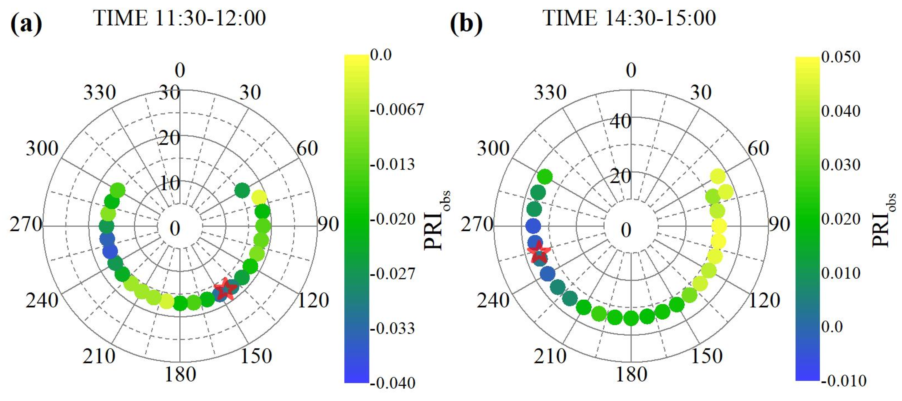
3.1. Estimation of LUE Using Multi-Angle Observed PRI

The observed PRI (PRIobs) changed with the viewing azimuth angles and its angular pattern differed with the solar position at a varied time on DOY 204 (a sunny day) (Figure 2). Within 30 min, solar radiation and solar position were near constant and the variations of PRI were a result of the different parts of the maize canopy viewed at different angles. We found that PRIobs obtained from 14:30 to 15:00 were much higher than that obtained closer to noon (11:30 to 12:00). PRIobs values in hotspot directions appeared lower than those when observer and the sun were far apart. These differences were more obvious in the afternoon hours than that at noon. The hotspot direction was in the same direction as the sun, resulting in more sunlit leaves being observed in the hotspot direction.
Using the multi-angle observations, we compared the observed PRI in the single view angle (PRIs, VAA = 180°) and the canopy PRI with multi-angle mean values (PRIcan) with LUEEC (Figure 3). Both PRIs and PRIcan showed similar diurnal variations to LUEEC. LUEEC, PRIs, and PRIcan decreased from sunrise and reached their minimum at noon than increased until the sunset. PRIcan (R2 = 0.49, p < 0.01) had a stronger correlation with LUEEC than PRIs (R2 = 0.41, p < 0.01). The PRIcan, which was the mean value of the multi-angle PRIobs, performed better in estimating LUE with tens of measurements evenly distributed at different view angles.

3.2. Performance of the PRI-Based LUE Model and SIF-Based Linear Model for GPP Estimation

The PRI-based LUE model and SIF-based linear model for GPP estimation were compared at different time scales. The summary statistics of both models are shown in Table 1. Significant relationships were found between LUEPRI × APAR and GPPEC at these three-time scales. The R2 between LUEPRI×APAR and GPPEC at the “daily mean” scale and the “30 min” scale was lower than that at the “day-by-day” scale (R2 = 0.71 ± 0.22, p < 0.01). This indicated that LUEPRI × APAR tracked the diurnal variations of GPPEC better than the seasonal variations of GPPEC. Compared to SIFcan, the LUEPRI×APAR was higher R2 with GPPEC at the short-term time scale, especially at the “day-by-day” scale. However, the R2 between SIFcan and GPPEC at the “daily mean” scale (R2 = 0.50, p < 0.001) was highest among the three time scales and higher than the R2 between LUEPRI×APAR and GPPEC (R2 = 0.44, p < 0.001) at the same time scale.
Figure 4 showed the day-by-day variation of R2 between LUEPRI × APAR and GPPEC (R2PRI), and between SIFcan and GPPEC (R2SIF) and their relative frequency. There was some data loss (Figure 4) because of instrument failure. Significant correlations (p < 0.05) between LUEPRI×APAR and GPPEC occurred on all 51 available days with an R2 ranging from 0.23–0.96. SIFcan showed significant relationships with GPPEC on 81% of the 79 available days (R2: 0.18–0.85). The highest frequency of R2PRI was 0.8–0.9, much higher than that of R2SIF (0.2–0.5). In summary, LUEPRI×APAR tracked the diurnal variations of GPPEC better than SIFcan for individual days.

3.3. Effects of Different Environmental Variables on the Abilities of the PRI-Based and SIF-Based Models in Tracking Diurnal Variations of GPP

Figure 5 illustrates the seasonal variations of the environmental variables, GPPEC and LUEEC. PAR and Q exhibited the largest day-to-day variations and high Q usually occurred with high PAR (Figure 5a). The day-to-day variation of RH appeared opposite those of PAR, while the several abrupt changes of SWC depended on irrigation and precipitation (Figure 5b). Both Ta and Ts remained around 30 °C during DOY 180–220, and then slowly decreased to around 22 °C at the end of the growing season (Figure 5c). The day-to-day fluctuation of Ta was larger than that of Ts (Figure 5c). The maize canopy showed pronounced seasonal variations in GPPEC and LUEEC (Figure 5d). The onset of GPPEC occurred on DOY 167, several days after emergence. GPPEC increased with maize development and reached its peak of 60 μmol CO2 m−2·s−1 on around DOY 215. During the early reproductive stage, GPPEC had high and stable values, sometimes dropped to low values due to low PAR. GPPEC decreased with leaf senescence at the end of the growing season. LUEEC increased from the start of the growing season, reaching the maximum on around DOY 190, and remaining until the early reproductive stage, and then decreasing.
To avoid the interactions between environmental variables, a random forest regression analysis was used to assess the effects of environmental variables on R2PRI and R2SIF. Among the environmental variables, the most important one affecting R2PRI was RH, with the percentages increase in mean square error (%IncMSE) of 25.6%. Ts (%IncMSE = 22.0%) was the second most important environmental variable affecting R2PRI followed by SWC (%IncMSE = 13.9%). PAR and Q were the least important variables (Figure 6a). Obvious differences were found between R2SIF and those of R2PRI. PAR appeared to be the most important driver for R2SIF (%IncMSE = 22.3%). Q was of secondary importance to R2SIF (%IncMSE = 11.5%) (Figure 6b).

3.4. Comparison between the Abilities of the PRI-Based and SIF-Based Models under Different Environmental Variables

R2PRI and R2SIF were compared under classified ranges of the environmental variables (Figure 7). R2PRI remained constant (>0.6) with the increase of PAR and Q (Figure 7a). R2SIF increased with the increase of the light-related variables (i.e., PAR and Q) and reached the highest values of 0.56 and 0.85 for the PAR range of 800–1000 μmol·m−2·s−1 and the Q range of >2, respectively (Figure 7a,b). R2SIF was higher than R2PRI for the Q range of >2 (Figure 7b).
The distributions of R2PRI and R2SIF were different for the two water-related variables (i.e., RH and SWC) (Figure 7c,d). R2PRI was conspicuously lower in RH < 60% than that in RH > 60%. It reached the highest value of 0.83 for the RH range of 70–80%. R2PRI had high values at low and high ends of SWC with a high value of 0.88 for the SWC range of 0.2–0.25 m3 m−3 and a high value of 0.81 for the SWC range of 0.4–0.5 m3 m−3. However, R2SIF fluctuated with the increase of RH and SWC.
For the temperature-related variables (Ta and Ts), the distributions of R2PRIand R2SIFalso differed (Figure 7e,f). The higher soil temperature showed the higher R2PRI. The highest R2PRI was at the temperature range of 31–34 °C, while the highest R2SIF was at the temperature range of 25–28 °C.
Overall, R2PRI was higher at high RH or under soil water stress (i.e., SWC too low or too high) or high temperature, while the higher R2SIF occurred under high solar radiation or clear sky. The PRI-based LUE model exhibited better performance than the SIF-based linear model in estimating GPP in most of the classified ranges of the environmental variables, with the SIF-based linear model performed slightly better under clear sky (Q > 2).

4. Discussion

4.1. Evaluation of Multi-Angle Observed PRI

This study found that the averages of the multi-angle observed PRI within short time intervals better represented the condition of the entire canopy in estimating LUE than the single angle observed PRI (Figure 3). This relationship indicates that the utilization of multi-angle observations with tens of measurements evenly distributed at different angles could diminish the angular effects to some extent. Crop canopies are non-Lambertian characterized by bidirectional reflection. Their reflectance changes because of the varied fraction of sunlit/shaded elements of the canopy with the changing angles. The reflectance at 531 nm differed significantly over sunlit and shaded elements of the canopy. The canopy elements whose reflectance differed as a function of illumination intensity lead to the variation in the PRI signal viewed at varied angles [25]. The sunlit elements are more likely to be exposed to excess light levels, causing a conversion of violaxanthin to zeaxanthin and resulting in a lowering of PRI. The angular effects of the observed PRI were also reported by Hilker et al. [49] and Zhang et al. [18], which was consistent with our observations (Figure 2). We used the simple arithmetic averages of the multi-angle observed PRI to represent the whole canopy with assuming the canopy as a big leaf in this study. There are also two-leaf approaches that interpreted the variations of the observed PRI with the sun-view geometry and canopy structure as their sensitivity to the fractions of sunlit/shaded leaves. Zhang et al. [58] used a two-leaf model to derive canopy PRI with multi-angle observations and found the two-leaf PRI could effectively improve the ability for indicating LUE over the big-leaf PRI in a subtropical evergreen coniferous forest. However, the canopy of maize was relatively homogeneous compared to the coniferous forest with more species. Different from the previous observation methods, the view zenith angle in this study was assigned to be consistent with the SZA, while the VAAs within half an hour were evenly distributed (Figure 2). Therefore, the arithmetic average was chosen as a more simple approach to reduce the angular effect in this study.

4.2. Comparison of the PRI-Based and the SIF-Based Models in Estimating Diurnal and Seasonal GPP Variations

Among different time scales, we found that the PRI-based LUE model exhibited better performance than the SIF-based linear model in estimating the diurnal variations of GPPEC, while the SIF-based linear model performed better at estimating the seasonal variations of GPPEC (Table 1, Figure 4). PRI may be a good indicator of LUE because of the link between PRI and xanthophyll cycle activity. The rapid xanthophyll cycle activity represented physiological regulations of photosynthesis on short-term changes in general environmental conditions and thus PRI was regarded as an optical indicator of LUE at diurnal time scales. Several studies have confirmed that the long-term (seasonal) PRI responses were primarily driven by constitutive changes in pigment pools (i.e., the ratio of carotenoid and chlorophyll) instead of facultative xanthophyll cycle activity [27,28,29,59,60]. Although the slower or seasonal pigment pool size adjustments of photosynthesis were also shown to correlate with LUE, the mechanistic explanations of the relationships differed [31]. Thus, the PRI-based LUE model showed a high advantage in the estimation of the diurnal photosynthesis variations, but a lower advantage in estimating the seasonal photosynthesis variations. Maize is a C4 plant, which does not have the photosynthetic “lunch break” phenomenon under high light at noon. Thus, the distribution of absorbed light energy relies on non-photochemical quenching (NPQ), i.e., heat energy dissipation through the xanthophyll cycle, which may be more conducive to the expression of the diurnal LUE variations by PRI. In contrast, it has been found that the relationship between SIF and GPP appears to be linear under stress conditions precisely due to the reduced SIF values around midday [45]. At the seasonal scale, considerable evidence based on retrievals from satellite [32,33,37,41,42] and ground-based measurements [43,44,61,62] has been showing strong empirical linear SIF-GPP relationships. In contrast, the studies conducted at short time scales (e.g., sub-daily) found insignificant relationship (R2 ≤ 0.3) than that in seasonal scale studies [63], which may be nonlinear [64]. Yang et al. [46] demonstrated that SIF primarily responded to changes in APAR rather than GPP and emphasized the needs of LUE information when estimating GPP at a short-term scale.

4.3. Environmental Effects on the Abilities of the PRI-Based and SIF-Based Models in Estimating GPP

In our study, RH was the most limiting factor for the PRI-based LUE model in estimating GPP of maize (Figure 6). Previous studies have reported that PRI has the highest and most common correlation with LUE under cloudless or slightly cloudy conditions, rather than water-limited conditions [19,58]. Our study demonstrated that the incident radiation (PAR) and sky condition (Q) were not influenced the performance of the PRI-based LUE model in estimating GPP (Figure 7a,b) because the APAR included in the model partly account for the sky radiation. The relationship between LUEPRI×APAR and GPPEC had a lower correlation when RH was lower than 60% (Figure 7c), which was consistent with the VPD-limited conditions in Zhang et al. [58]. However, in the cropland with irrigation, SWC was not a limitation. We infer that the PRI-based LUE model was more sensitive to the atmospheric water deficit (low RH) than the soil water deficit (low SWC) because the former had a direct effect on opening and closing of the leaf stomata and then the photosynthesis, not the reflectance of the leaf and canopy. Soil temperature also had a positive effect on the PRI-based LUE model (Figure 6a and Figure 7f). The high Ts occurred at the late V stages (DOY 195 to 207) with synchronously high RH (Figure 5). Thus, the maize rapid grown at this stage had a higher photosynthetic rate and linear energy distribution, leading to the good performance of the PRI-based LUE model.
Different from the PRI-based LUE model, the relationship between SIFcan and GPPEC was influenced by the light-related factors, i.e., PAR and Q. It was found that incident radiation played dominant roles in SIF changes among environmental variables by sensitivity tests on simulated SIF data by Soil Canopy Observation Photosynthesis Energy (SCOPE) model [65]. Photosynthesis and chlorophyll fluorescence were highly correlated when vegetation was exposed to excess incident radiation [38]. The incident radiation absorbed by chlorophyll was a key driver of both GPP and SIF, but limited or saturated light conditions could result in different coupling patterns between the efficiency of photosynthesis and fluorescence [66,67]. Due to the effect of diffuse radiation, the clearer the sky showed the stronger correlation between SIF and GPP for maize canopy in our study (Figure 7). This finding was in agreement with Miao et al. [66], but differed from Yang et al. [46], Goulas et al. [68], and Li et al. [50].

4.4. Combination of PRI and SIF for GPP Estimation

Photosynthesis, fluorescence, and NPQ are three pathways to dissipate the absorbed light energy, which interrelate and compete with each other. The relationship between photochemical yield (ΦP) and fluorescence yield (ΦF) is divided into two distinct phases: under high light, NPQ dominates the variations of ΦP, with constant photochemical quenching (PQ); under low light, the variations of ΦP are mainly driven by PQ, with constantly low NPQ [67]. ΦP is in proportion to ΦF under the NPQ stage and becomes inversely proportional under the PQ stage because of the opposite effects on ΦF with decreasing PQ and increasing NPQ. PRI has been proven to be a representative of the temporal dynamics of NPQ [69]. The combination of PRI and SIF observations could be a solution for a better estimation of photosynthesis. Cheng et al. [63]) and Schickling et al. [70] combined the PRI and SIF data in simple linear regression models and found that their combinations improved the estimation of GPP. However, their models were more mathematical than mechanistic. Atherton et al. [71] combined PRI and SIF via NPQ model and ΦF to predict the dynamics of photosynthetic efficiency at leaf scale and short-time scale from a theoretical perspective. Different from their direct combination of PRI and SIF, we treated SIF and PRI as alternatives for the estimation of GPP and pointed out the better performance of the PRI-based LUE model under most environmental conditions for the maize field in our study. Additional studies on the theoretical combination of PRI and SIF at various temporal and spatial scales would be helpful for a more accurate estimation of GPP.

5. Conclusions

In this study, we measured multi-angular canopy spectra continuously during the whole 2018 growing season of a maize field. We compared the ability of the single-angle and multi-angle PRI observations at canopy level in estimating LUE. Then, the PRI-based LUE model was evaluated and compared to the SIF-based linear model for their performance in the estimation of GPP during the maize growing season in 2018. The major results are as follows:
(1)
the observed PRI varied with sun-view angles and the averaged PRI using the multi-angle observations within a short time exhibited better performance than single-angle observed PRI in the estimation of LUE in the maize field;
(2)
LUEPRI×APAR tracked the variations of GPP during the growing season of the maize field in 2018, and it demonstrated a higher ability to capture the diurnal variations of GPP, while SIF was a better fit for the seasonal variations of GPP;
(3)
RH was the most important factor affecting the utilization of the PRI-based LUE model to estimate diurnal GPP variations, while PAR affected most for the SIF-based linear model. Under most environmental conditions, the performance of the SIF-based linear model was not as good as the PRI-based LUE model except for clear days (Q > 2).

Author Contributions

Conceptualization, J.C., S.W., and B.C.; methodology, J.C., B.C., and Q.Z.; formal analysis, J.C. and L.M.; investigation, Q.Z., Z.L., X.Z., and Y.W.; writing—original draft preparation, J.C.; writing—review and editing, Q.Z., S.W., B.C, Y.Z., and R.A.M.; visualization, J.C.; supervision, S.W. and Y.Z.; funding acquisition, S.W., Y.Z., and Q.Z. All authors have read and agreed to the published version of the manuscript.

Funding

This research was funded by the National Key Research and Development Program of China, grant number 2017YFC0503803; the National Natural Science Foundation of China, grant number 41571192 and 41701393; and the Natural Science Foundation of Jiangsu Province for Youth, grant number BK20170641. Q.Z. was supported by the China Scholarship Council (CSC), grant number 201906195015.

Conflicts of Interest

The authors declare no conflict of interest.

References

  1. Le Quéré, C.; Raupach, M.R.; Canadell, J.G.; Marland, G.; Bopp, L.; Ciais, P.; Conway, T.J.; Doney, S.C.; Feely, R.A.; Foster, P.; et al. Trends in the sources and sinks of carbon dioxide. Nat. Geosci. 2009, 2, 831–836. [Google Scholar] [CrossRef]
  2. Xia, J.; Niu, S.; Ciais, P.; Janssens, I.A.; Chen, J.; Ammann, C.; Arain, A.; Blanken, P.D.; Cescatti, A.; Bonal, D.; et al. Joint control of terrestrial gross primary productivity by plant phenology and physiology. Proc. Natl. Acad. Sci. USA 2015, 112, 2788–2793. [Google Scholar] [CrossRef] [PubMed] [Green Version]
  3. Beer, C.; Reichstein, M.; Tomelleri, E.; Ciais, P.; Jung, M.; Carvalhais, N.; Rödenbeck, C.; Arain, M.A.; Baldocchi, D.; Bonan, G.B.; et al. Terrestrial gross carbon dioxide uptake: Global distribution and covariation with climate. Science 2010, 329, 834–838. [Google Scholar] [CrossRef] [PubMed] [Green Version]
  4. Forkel, M.; Carvalhais, N.; Rödenbeck, C.; Keeling, R.; Heimann, M.; Thonicke, K.; Zaehle, S.; Reichstein, M. Enhanced seasonal CO2 exchange caused by amplified plant productivity in northern ecosystems. Science 2016, 351, 696–699. [Google Scholar] [CrossRef] [PubMed] [Green Version]
  5. Graven, H.; Keeling, R.; Piper, S.; Patra, P.; Stephens, B.; Wofsy, S.; Welp, L.; Sweeney, C.; Tans, P.; Kelley, J.; et al. Enhanced seasonal exchange of CO2 by northern ecosystems since 1960. Science 2013, 341, 1085–1089. [Google Scholar] [CrossRef] [Green Version]
  6. Poulter, B.; Frank, D.; Ciais, P.; Myneni, R.B.; Andela, N.; Bi, J.; Broquet, G.; Canadell, J.G.; Chevallier, F.; Liu, Y.Y.; et al. Contribution of semi-arid ecosystems to interannual variability of the global carbon cycle. Nature 2014, 509, 600–603. [Google Scholar] [CrossRef] [Green Version]
  7. Drolet, G.; Middleton, E.; Huemmrich, K.; Hall, F.; Amiro, B.; Barr, A.; Black, T.; McCaughey, J.; Margolis, H. Regional mapping of gross light-use efficiency using MODIS spectral indices. Remote Sens. Environ. 2008, 112, 3064–3078. [Google Scholar] [CrossRef]
  8. Damm, A.; Elbers, J.; Erler, A.; Gioli, B.; Hamdi, K.; Hutjes, R.; Kosvancova, M.; Meroni, M.; Miglietta, F.; Moersch, A.; et al. Remote sensing of sun-induced fluorescence to improve modeling of diurnal courses of gross primary production (GPP). Glob. Chang. Biol. 2010, 16, 171–186. [Google Scholar] [CrossRef]
  9. Yuan, W.; Liu, S.; Zhou, G.; Zhou, G.; Tieszen, L.L.; Baldocchi, D.; Bernhofer, C.; Gholz, H.; Goldstein, A.H.; Goulden, M.L.; et al. Deriving a light use efficiency model from eddy covariance flux data for predicting daily gross primary production across biomes. Agric. For. Meteorol. 2007, 143, 189–207. [Google Scholar] [CrossRef] [Green Version]
  10. Yuan, W.; Cai, W.; Xia, J.; Chen, J.; Liu, S.; Dong, W.; Merbold, L.; Law, B.; Arain, A.; Beringer, J.; et al. Global comparison of light use efficiency models for simulating terrestrial vegetation gross primary production based on the LaThuile database. Agric. For. Meteorol. 2014, 192, 108–120. [Google Scholar] [CrossRef]
  11. Running, S.W.; Thornton, P.E.; Nemani, R.; Glassy, J.M. Global terrestrial gross and net primary productivity from the earth observing system. In Methods in Ecosystem Science; Springer: Berlin/Heidelberg, Germany, 2000; pp. 44–57. [Google Scholar]
  12. Potter, C.S.; Randerson, J.T.; Field, C.B.; Matson, P.A.; Vitousek, P.M.; Mooney, H.A.; Klooster, S.A. Terrestrial ecosystem production: A process model based on global satellite and surface data. Glob. Biogeochem. Cycles 1993, 7, 811–841. [Google Scholar] [CrossRef]
  13. Knyazikhin, Y.; Martonchik, J.; Myneni, R.B.; Diner, D.; Running, S.W. Synergistic algorithm for estimating vegetation canopy leaf area index and fraction of absorbed photosynthetically active radiation from MODIS and MISR data. J. Geophys. Res. Atmos. 1998, 103, 32257–32275. [Google Scholar] [CrossRef] [Green Version]
  14. Chen, M.J. Canopy architecture and remote sensing of the fraction of photosynthetically active radiation absorbed by boreal conifer forests. IEEE Trans. Geosci. Remote Sens. 1996, 34, 1353–1368. [Google Scholar] [CrossRef]
  15. Stagakis, S.; Markos, N.; Sykioti, O.; Kyparissis, A. Tracking seasonal changes of leaf and canopy light use efficiency in a Phlomis fruticosa Mediterranean ecosystem using field measurements and multi-angular satellite hyperspectral imagery. ISPRS J. Photogramm. Remote Sens. 2014, 97, 138–151. [Google Scholar] [CrossRef]
  16. Garbulsky, M.F.; Peñuelas, J.; Gamon, J.; Inoue, Y.; Filella, I. The photochemical reflectance index (PRI) and the remote sensing of leaf, canopy and ecosystem radiation use efficiencies: A review and meta-analysis. Remote Sens. Environ. 2011, 115, 281–297. [Google Scholar] [CrossRef]
  17. Gamon, J.; Penuelas, J.; Field, C. A narrow-waveband spectral index that tracks diurnal changes in photosynthetic efficiency. Remote Sens. Environ. 1992, 41, 35–44. [Google Scholar] [CrossRef]
  18. Zhang, Q.; Ju, W.; Chen, J.M.; Wang, H.; Yang, F.; Fan, W.; Huang, Q.; Zheng, T.; Feng, Y.; Zhou, Y.; et al. Ability of the photochemical reflectance index to track light use efficiency for a sub-tropical planted coniferous forest. Remote Sens. 2015, 7, 16938–16962. [Google Scholar] [CrossRef] [Green Version]
  19. Soudani, K.; Hmimina, G.; Dufrêne, E.; Berveiller, D.; Delpierre, N.; Ourcival, J.-M.; Rambal, S.; Joffre, R. Relationships between photochemical reflectance index and light-use efficiency in deciduous and evergreen broadleaf forests. Remote Sens. Environ. 2014, 144, 73–84. [Google Scholar] [CrossRef]
  20. Nakaji, T.; Oguma, H.; Fujinuma, Y. Seasonal changes in the relationship between photochemical reflectance index and photosynthetic light use efficiency of Japanese larch needles. Int. J. Remote Sens. 2006, 27, 493–509. [Google Scholar] [CrossRef]
  21. Nakaji, T.; Kosugi, Y.; Takanashi, S.; Niiyama, K.; Noguchi, S.; Tani, M.; Oguma, H.; Nik, A.R. Estimation of light-use efficiency through a combinational use of the photochemical reflectance index and vapor pressure deficit in an evergreen tropical rainforest at Pasoh, Peninsular Malaysia. Remote Sens. Environ. 2014, 150, 82–92. [Google Scholar] [CrossRef] [Green Version]
  22. Drolet, G.G.; Huemmrich, K.F.; Hall, F.G.; Middleton, E.M.; Black, T.A.; Barr, A.G.; Margolis, H.A. A MODIS-derived photochemical reflectance index to detect inter-annual variations in the photosynthetic light-use efficiency of a boreal deciduous forest. Remote Sens. Environ. 2005, 98, 212–224. [Google Scholar] [CrossRef]
  23. Barton, C.V.M.; North, P. Remote sensing of canopy light use efficiency using the photochemical reflectance index: Model and sensitivity analysis. Remote Sens. Environ. 2001, 78, 264–273. [Google Scholar] [CrossRef]
  24. Damm, A.; Guanter, L.; Verhoef, W.; Schläpfer, D.; Garbari, S.; Schaepman, M.E. Impact of varying irradiance on vegetation indices and chlorophyll fluorescence derived from spectroscopy data. Remote Sens. Environ. 2015, 156, 202–215. [Google Scholar] [CrossRef]
  25. Hall, F.G.; Hilker, T.; Coops, N.C.; Lyapustin, A.; Huemmrich, K.F.; Middleton, E.; Margolis, H.; Drolet, G.; Black, T.A. Multi-angle remote sensing of forest light use efficiency by observing PRI variation with canopy shadow fraction. Remote Sens. Environ. 2008, 112, 3201–3211. [Google Scholar] [CrossRef] [Green Version]
  26. Verrelst, J.; Schaepman, M.E.; Koetz, B.; Kneubühler, M. Angular sensitivity analysis of vegetation indices derived from CHRIS/PROBA data. Remote Sens. Environ. 2008, 112, 2341–2353. [Google Scholar] [CrossRef]
  27. Filella, I.; Porcar-Castell, A.; Munné-Bosch, S.; Bäck, J.; Garbulsky, M.; Peñuelas, J. PRI assessment of long-term changes in carotenoids/chlorophyll ratio and short-term changes in de-epoxidation state of the xanthophyll cycle. Int. J. Remote Sens. 2009, 30, 4443–4455. [Google Scholar] [CrossRef]
  28. Wong, C.Y.; Gamon, J.A. Three causes of variation in the photochemical reflectance index (PRI) in evergreen conifers. New Phytol. 2015, 206, 187–195. [Google Scholar] [CrossRef]
  29. Wong, C.Y.; Gamon, J.A. The photochemical reflectance index provides an optical indicator of spring photosynthetic activation in evergreen conifers. New Phytol. 2015, 206, 196–208. [Google Scholar] [CrossRef]
  30. Gitelson, A.A.; Gamon, J.A.; Solovchenko, A. Multiple drivers of seasonal change in PRI: Implications for photosynthesis 1. Leaf level. Remote Sens. Environ. 2017, 190, 110–116. [Google Scholar] [CrossRef] [Green Version]
  31. Gitelson, A.A.; Gamon, J.A.; Solovchenko, A. Multiple drivers of seasonal change in PRI: Implications for photosynthesis 2. Stand level. Remote Sens. Environ. 2017, 190, 198–206. [Google Scholar] [CrossRef] [Green Version]
  32. Frankenberg, C.; Fisher, J.B.; Worden, J.; Badgley, G.; Saatchi, S.S.; Lee, J.E.; Toon, G.C.; Butz, A.; Jung, M.; Kuze, A.; et al. New global observations of the terrestrial carbon cycle from GOSAT: Patterns of plant fluorescence with gross primary productivity. Geophys. Res. Lett. 2011, 38. [Google Scholar] [CrossRef] [Green Version]
  33. Guanter, L.; Frankenberg, C.; Dudhia, A.; Lewis, P.E.; Gómez-Dans, J.; Kuze, A.; Suto, H.; Grainger, R.G. Retrieval and global assessment of terrestrial chlorophyll fluorescence from GOSAT space measurements. Remote Sens. Environ. 2012, 121, 236–251. [Google Scholar] [CrossRef]
  34. Li, X.; Xiao, J.; He, B. Chlorophyll fluorescence observed by OCO-2 is strongly related to gross primary productivity estimated from flux towers in temperate forests. Remote Sens. Environ. 2018, 204, 659–671. [Google Scholar] [CrossRef]
  35. Li, X.; Xiao, J.; He, B.; Altaf Arain, M.; Beringer, J.; Desai, A.R.; Emmel, C.; Hollinger, D.Y.; Krasnova, A.; Mammarella, I.; et al. Solar-induced chlorophyll fluorescence is strongly correlated with terrestrial photosynthesis for a wide variety of biomes: First global analysis based on OCO-2 and flux tower observations. Glob. Chang. Biol. 2018, 24, 3990–4008. [Google Scholar] [CrossRef] [PubMed]
  36. Sun, Y.; Frankenberg, C.; Jung, M.; Joiner, J.; Guanter, L.; Köhler, P.; Magney, T. Overview of Solar-Induced chlorophyll Fluorescence (SIF) from the Orbiting Carbon Observatory-2: Retrieval, cross-mission comparison, and global monitoring for GPP. Remote Sens. Environ. 2018, 209, 808–823. [Google Scholar] [CrossRef]
  37. Zhang, Y.; Xiao, X.; Jin, C.; Dong, J.; Zhou, S.; Wagle, P.; Joiner, J.; Guanter, L.; Zhang, Y.; Zhang, G.; et al. Consistency between sun-induced chlorophyll fluorescence and gross primary production of vegetation in North America. Remote Sens. Environ. 2016, 183, 154–169. [Google Scholar] [CrossRef] [Green Version]
  38. Baker, N.R. Chlorophyll fluorescence: A probe of photosynthesis in vivo. Annu. Rev. Plant Biol. 2008, 59, 89–113. [Google Scholar] [CrossRef] [Green Version]
  39. Meroni, M.; Rossini, M.; Guanter, L.; Alonso, L.; Rascher, U.; Colombo, R.; Moreno, J. Remote sensing of solar-induced chlorophyll fluorescence: Review of methods and applications. Remote Sens. Environ. 2009, 113, 2037–2051. [Google Scholar] [CrossRef]
  40. Zarco-Tejada, P.J.; Morales, A.; Testi, L.; Villalobos, F.J. Spatio-temporal patterns of chlorophyll fluorescence and physiological and structural indices acquired from hyperspectral imagery as compared with carbon fluxes measured with eddy covariance. Remote Sens. Environ. 2013, 133, 102–115. [Google Scholar] [CrossRef]
  41. Joiner, J.; Yoshida, Y.; Vasilkov, A.; Schaefer, K.; Jung, M.; Guanter, L.; Zhang, Y.; Garrity, S.; Middleton, E.; Huemmrich, K.; et al. The seasonal cycle of satellite chlorophyll fluorescence observations and its relationship to vegetation phenology and ecosystem atmosphere carbon exchange. Remote Sens. Environ. 2014, 152, 375–391. [Google Scholar] [CrossRef] [Green Version]
  42. Wagle, P.; Zhang, Y.; Jin, C.; Xiao, X. Comparison of solar-induced chlorophyll fluorescence, light-use efficiency, and process-based GPP models in maize. Ecol. Appl. 2016, 26, 1211–1222. [Google Scholar] [CrossRef] [PubMed] [Green Version]
  43. Yang, H.; Yang, X.; Zhang, Y.; Heskel, M.A.; Lu, X.; Munger, J.W.; Sun, S.; Tang, J. Chlorophyll fluorescence tracks seasonal variations of photosynthesis from leaf to canopy in a temperate forest. Glob. Chang. Biol. 2017, 23, 2874–2886. [Google Scholar] [CrossRef] [PubMed]
  44. Yang, X.; Tang, J.; Mustard, J.F.; Lee, J.E.; Rossini, M.; Joiner, J.; Munger, J.W.; Kornfeld, A.; Richardson, A.D. Solar-induced chlorophyll fluorescence that correlates with canopy photosynthesis on diurnal and seasonal scales in a temperate deciduous forest. Geophys. Res. Lett. 2015, 42, 2977–2987. [Google Scholar] [CrossRef]
  45. Paul-Limoges, E.; Damm, A.; Hueni, A.; Liebisch, F.; Eugster, W.; Schaepman, M.E.; Buchmann, N. Effect of environmental conditions on sun-induced fluorescence in a mixed forest and a cropland. Remote Sens. Environ. 2018, 219, 310–323. [Google Scholar] [CrossRef]
  46. Yang, K.; Ryu, Y.; Dechant, B.; Berry, J.A.; Hwang, Y.; Jiang, C.; Kang, M.; Kim, J.; Kimm, H.; Kornfeld, A.; et al. Sun-induced chlorophyll fluorescence is more strongly related to absorbed light than to photosynthesis at half-hourly resolution in a rice paddy. Remote Sens. Environ. 2018, 216, 658–673. [Google Scholar] [CrossRef]
  47. Baldocchi, D.D. Assessing the eddy covariance technique for evaluating carbon dioxide exchange rates of ecosystems: Past, present and future. Glob. Chang. Biol. 2003, 9, 479–492. [Google Scholar] [CrossRef] [Green Version]
  48. Reichstein, M.; Falge, E.; Baldocchi, D.; Papale, D.; Aubinet, M.; Berbigier, P.; Bernhofer, C.; Buchmann, N.; Gilmanov, T.; Granier, A.; et al. On the separation of net ecosystem exchange into assimilation and ecosystem respiration: Review and improved algorithm. Glob. Chang. Biol. 2005, 11, 1424–1439. [Google Scholar] [CrossRef]
  49. Hilker, T.; Coops, N.C.; Hall, F.G.; Black, T.A.; Wulder, M.A.; Nesic, Z.; Krishnan, P. Separating physiologically and directionally induced changes in PRI using BRDF models. Remote Sens. Environ. 2008, 112, 2777–2788. [Google Scholar] [CrossRef] [Green Version]
  50. Li, Z.; Zhang, Q.; Li, J.; Yang, X.; Wu, Y.; Zhang, Z.; Wang, S.; Wang, H.; Zhang, Y. Solar-induced chlorophyll fluorescence and its link to canopy photosynthesis in maize from continuous ground measurements. Remote Sens. Environ. 2020, 236, 111420. [Google Scholar] [CrossRef]
  51. Zhang, Z.; Zhang, Y.; Zhang, Q.; Chen, J.M.; Porcar-Castell, A.; Guanter, L.; Wu, Y.; Zhang, X.; Wang, H.; Ding, D.; et al. Assessing bi-directional effects on the diurnal cycle of measured solar-induced chlorophyll fluorescence in crop canopies. Agric. For. Meteorol. 2020. [Google Scholar] [CrossRef]
  52. Zhan, C.; Zhang, Q.; Li, Z.; Zhang, X.; Wu, Y. Impacts of different radiometric calibration methods on the retrievals of sun-induced chlorophyll fluorescence and its relation to productivity for continuous field measurements. J. Appl. Remote Sens. 2019, 14, 022206. [Google Scholar] [CrossRef]
  53. Mazzoni, M.; Meroni, M.; Fortunato, C.; Colombo, R.; Verhoef, W. Retrieval of maize canopy fluorescence and reflectance by spectral fitting in the O2—A absorption band. Remote Sens. Environ. 2012, 124, 72–82. [Google Scholar] [CrossRef]
  54. Meroni, M.; Busetto, L.; Colombo, R.; Guanter, L.; Moreno, J.; Verhoef, W. Performance of spectral fitting methods for vegetation fluorescence quantification. Remote Sens. Environ. 2010, 114, 363–374. [Google Scholar] [CrossRef]
  55. Meroni, M.; Colombo, R. Leaf level detection of solar induced chlorophyll fluorescence by means of a subnanometer resolution spectroradiometer. Remote Sens. Environ. 2006, 103, 438–448. [Google Scholar] [CrossRef]
  56. Gill, D.A.; Mascia, M.B.; Ahmadia, G.N.; Glew, L.; Lester, S.E.; Barnes, M.; Craigie, I.; Darling, E.S.; Free, C.M.; Geldmann, J.; et al. Capacity shortfalls hinder the performance of marine protected areas globally. Nature 2017, 543, 665–669. [Google Scholar] [CrossRef] [PubMed]
  57. Huang, K.; Xia, J. High ecosystem stability of evergreen broadleaf forests under severe droughts. Glob. Chang. Biol. 2019, 25, 3494–3503. [Google Scholar] [CrossRef]
  58. Zhang, Q.; Chen, J.M.; Ju, W.; Wang, H.; Qiu, F.; Yang, F.; Fan, W.; Huang, Q.; Wang, Y.-p.; Feng, Y.; et al. Improving the ability of the photochemical reflectance index to track canopy light use efficiency through differentiating sunlit and shaded leaves. Remote Sens. Environ. 2017, 194, 1–15. [Google Scholar] [CrossRef]
  59. Gamon, J.A.; Berry, J.A. Facultative and constitutive pigment effects on the Photochemical Reflectance Index (PRI) in sun and shade conifer needles. Isr. J. Plant Sci. 2012, 60, 85–95. [Google Scholar] [CrossRef]
  60. Stylinski, C.; Gamon, J.; Oechel, W. Seasonal patterns of reflectance indices, carotenoid pigments and photosynthesis of evergreen chaparral species. Oecologia 2002, 131, 366–374. [Google Scholar] [CrossRef]
  61. Magney, T.S.; Bowling, D.R.; Logan, B.A.; Grossmann, K.; Stutz, J.; Blanken, P.D.; Burns, S.P.; Cheng, R.; Garcia, M.A.; Kӧhler, P.; et al. Mechanistic evidence for tracking the seasonality of photosynthesis with solar-induced fluorescence. Proc. Natl. Acad. Sci. USA 2019, 116, 11640–11645. [Google Scholar] [CrossRef] [Green Version]
  62. Rossini, M.; Meroni, M.; Migliavacca, M.; Manca, G.; Cogliati, S.; Busetto, L.; Picchi, V.; Cescatti, A.; Seufert, G.; Colombo, R. High resolution field spectroscopy measurements for estimating gross ecosystem production in a rice field. Agric. For. Meteorol. 2010, 150, 1283–1296. [Google Scholar] [CrossRef]
  63. Cheng, Y.-B.; Middleton, E.M.; Zhang, Q.; Huemmrich, K.F.; Campbell, P.K.; Cook, B.D.; Kustas, W.P.; Daughtry, C.S. Integrating solar induced fluorescence and the photochemical reflectance index for estimating gross primary production in a cornfield. Remote Sens. 2013, 5, 6857–6879. [Google Scholar] [CrossRef] [Green Version]
  64. Zarco-Tejada, P.J.; González-Dugo, M.; Fereres, E. Seasonal stability of chlorophyll fluorescence quantified from airborne hyperspectral imagery as an indicator of net photosynthesis in the context of precision agriculture. Remote Sens. Environ. 2016, 179, 89–103. [Google Scholar] [CrossRef]
  65. Verrelst, J.; Rivera, J.P.; van der Tol, C.; Magnani, F.; Mohammed, G.; Moreno, J. Global sensitivity analysis of the SCOPE model: What drives simulated canopy-leaving sun-induced fluorescence? Remote Sens. Environ. 2015, 166, 8–21. [Google Scholar] [CrossRef]
  66. Miao, G.; Guan, K.; Yang, X.; Bernacchi, C.J.; Berry, J.A.; DeLucia, E.H.; Wu, J.; Moore, C.E.; Meacham, K.; Cai, Y.; et al. Sun-induced chlorophyll fluorescence, photosynthesis, and light use efficiency of a soybean field from seasonally continuous measurements. J. Geophys. Res. Biogeosci. 2018, 123, 610–623. [Google Scholar] [CrossRef]
  67. Porcar-Castell, A.; Tyystjärvi, E.; Atherton, J.; van der Tol, C.; Flexas, J.; Pfündel, E.E.; Moreno, J.; Frankenberg, C.; Berry, J.A. Linking chlorophyll a fluorescence to photosynthesis for remote sensing applications: Mechanisms and challenges. J. Exp. Bot. 2014, 65, 4065–4095. [Google Scholar] [CrossRef]
  68. Goulas, Y.; Fournier, A.; Daumard, F.; Champagne, S.; Ounis, A.; Marloie, O.; Moya, I. Gross primary production of a wheat canopy relates stronger to far red than to red solar-induced chlorophyll fluorescence. Remote Sens. 2017, 9, 97. [Google Scholar] [CrossRef] [Green Version]
  69. Sukhova, E.; Sukhov, V. Connection of the photochemical reflectance index (PRI) with the photosystem II quantum yield and nonphotochemical quenching can be dependent on variations of photosynthetic parameters among investigated plants: A meta-analysis. Remote Sens. 2018, 10, 771. [Google Scholar] [CrossRef] [Green Version]
  70. Schickling, A.; Matveeva, M.; Damm, A.; Schween, J.H.; Wahner, A.; Graf, A.; Crewell, S.; Rascher, U. Combining sun-induced chlorophyll fluorescence and photochemical reflectance index improves diurnal modeling of gross primary productivity. Remote Sens. 2016, 8, 574. [Google Scholar] [CrossRef] [Green Version]
  71. Atherton, J.; Nichol, C.; Porcar-Castell, A. Using spectral chlorophyll fluorescence and the photochemical reflectance index to predict physiological dynamics. Remote Sens. Environ. 2016, 176, 17–30. [Google Scholar] [CrossRef]
Figure 1. Location of the study site at Shangqiu station, Henan province, China. Panel (a) was a satellite image of the maize field in our study area from Google Earth. (b) and (c) represented the location of the study site in Henan province and China, respectively.
Remotesensing 12 02812 g001
Figure 2. Photochemical reflectance index (PRI) observations in a polar coordinate system. The observed PRI (PRIobs) were obtained at different view angles at a different time on Day of Year (DOY) 204 (23 July, 2018). The red pentagram represents the average solar position within the 30 min in the polar coordinate system delineated by solar zenith angle and solar azimuth angle. Azimuth angles are defined from geodetic north.
Remotesensing 12 02812 g002
Figure 3. Linear regressions of half-hourly (a) single-angle observed PRI (PRIs) and light use efficiency based on eddy covariance (EC) measurement (LUEEC), (b) canopy PRI (PRIcan) and LUEEC, and (c) their diurnal variation on DOY 204 (23 July, 2018).
Remotesensing 12 02812 g003
Figure 4. Coefficients of determination between LUEPRI×APAR and GPPEC (R2PRI), SIFcan and GPPEC (R2SIF) on individual days and distribution of their relative frequency over the 2018 growing season of the maize field. (a) and (b) represented the R2PRI and its relative frequency respectively, while (c) and (d) represented the R2SIF and its relative frequency respectively.
Remotesensing 12 02812 g004
Figure 5. Seasonal variations of the daily mean (a) photosynthetically active radiation (PAR) and sky condition (Q), (b) relative humidity (RH), and soil water content (SWC), (c) air temperature (Ta) and soil temperature (Ts), and (d) GPPEC and LUEEC. Daily means were calculated from half-hourly values from 6:00 to 18:00 in the day. Small dot indicates half-hourly GPPEC.
Remotesensing 12 02812 g005
Figure 6. Relative contributions of the environmental variables for explaining (a) R2PRI, the correlation between LUEPRI×APAR and GPPEC, (b) R2SIF, the correlation between SIFcan and GPPEC.
Remotesensing 12 02812 g006
Figure 7. Distribution of R2PRI and R2SIF under the classified (a) PAR, (b) Q, (c) RH, (d) SWC, (e) Ta, (f) Ts. Error bars represent standard deviations of R2 under the classified ranges of the environmental variations.
Remotesensing 12 02812 g007
Table 1. Summary statistics of the photochemical reflectance index (PRI)-based light use efficiency (LUE) model and solar-induced fluorescence (SIF)-based linear model for gross primary production (GPP) estimation at different time scales.
Explanatory Terms for GPP Regression Model
Unit: μmol CO2 m−2·s−1
LUEPRI × APAR: GPPEC *SIFcan: GPPEC **
R2pRMSER2pRMSE
daily mean0.44<0.00112.250.50<0.00111.75
30 min0.47<0.00115.280.45<0.00116.12
day-by-day ***0.71 ± 0.220.00 ± 0.014.59 ± 3.080.38 ± 0.230.08 ± 0.198.90 ± 5.51
* LUEPRI = a × PRIcan + b, where a and b were fitted linearly using LUEEC and PRIcan over the half-hourly values from 6:00 to 18:00 each day during the entire growing season in 2018. GPPEC represented the EC measured GPP. ** SIFcan represented the canopy SIF. *** The results of “day-by-day” were the averages ± standard deviations of the statistical variables (coefficient of determination (R2), significant level (p), and root mean square error (RMSE)).

