Novel Machine Learning Approaches for Modelling the Gully Erosion Susceptibility

 , , ,
, , ,  , ,
, ,  ,
,  and
and
Abstract
:
1. Introduction
2. Materials and Methods
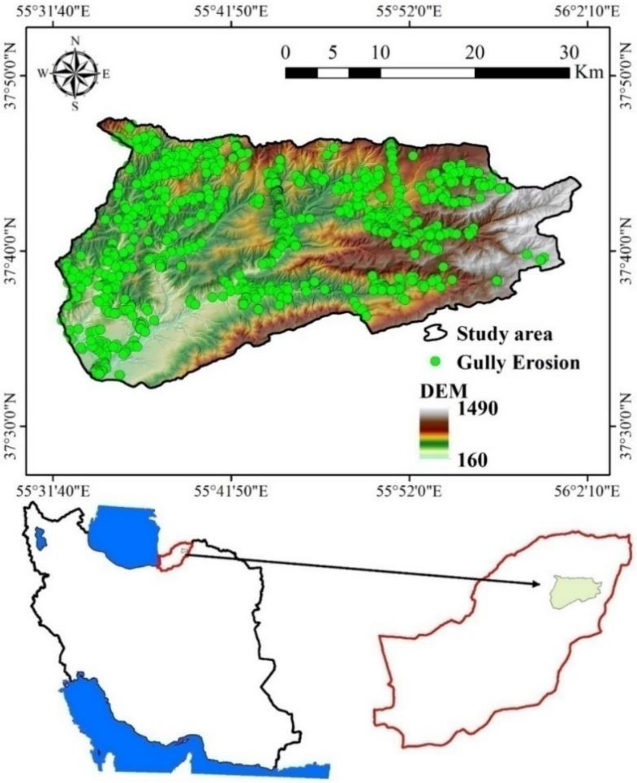
2.1. Study Area
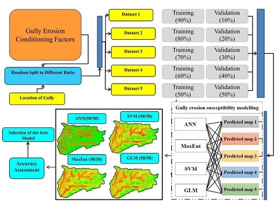
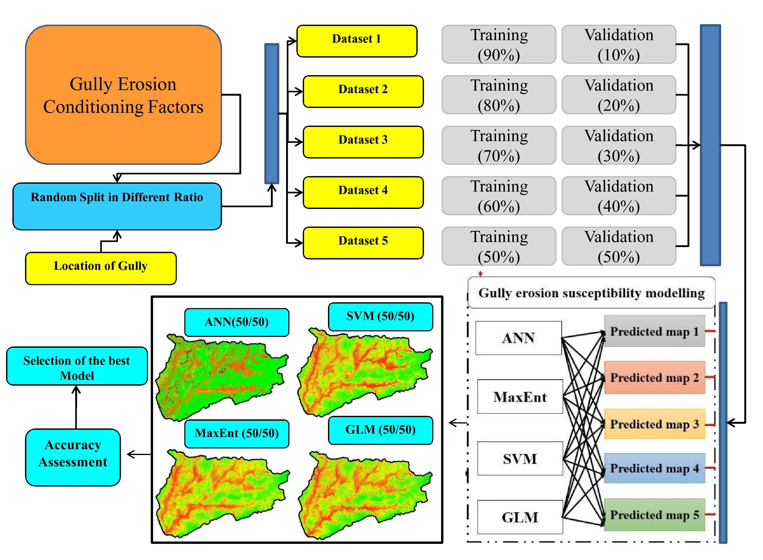
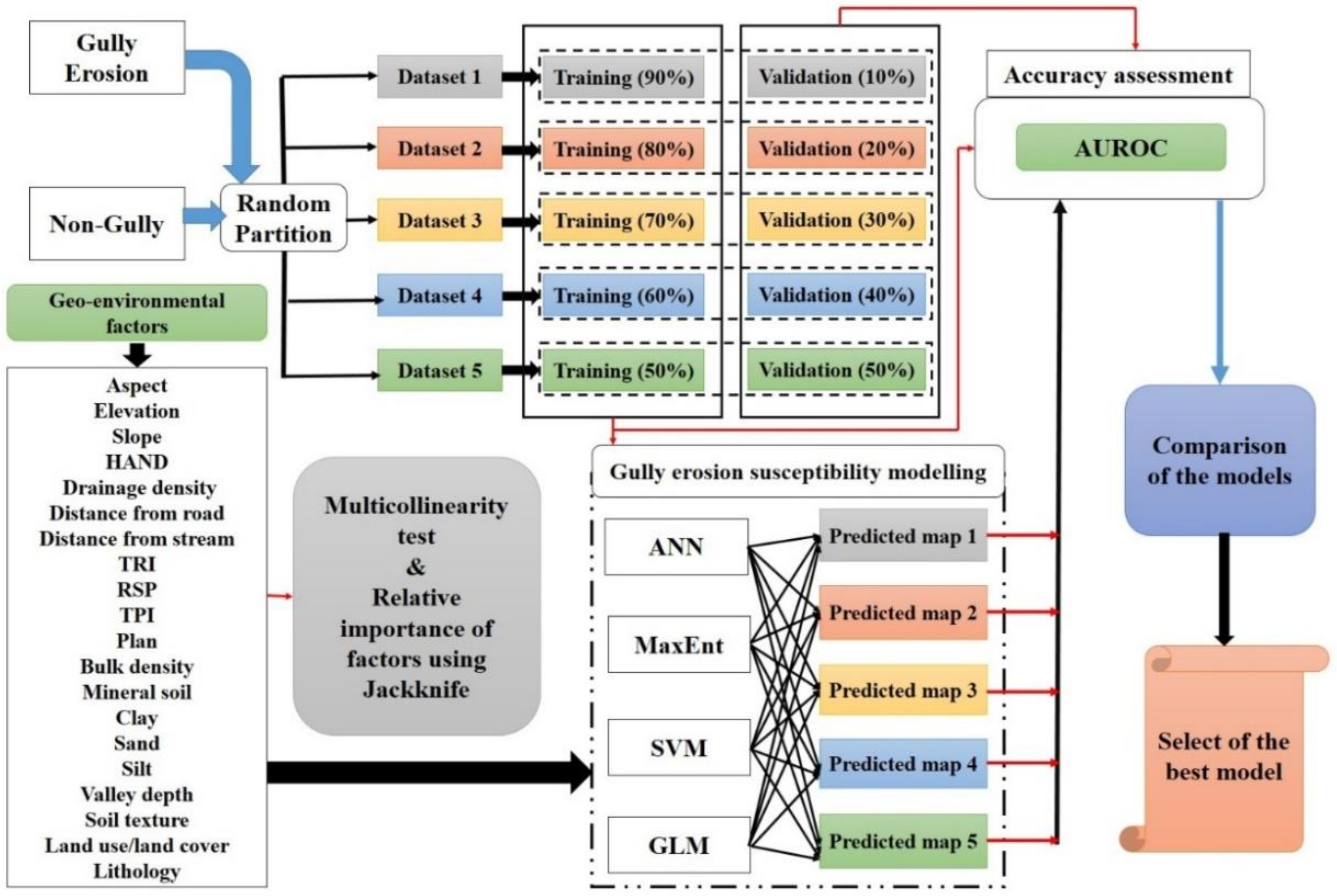
2.2. Methodology
- (i)
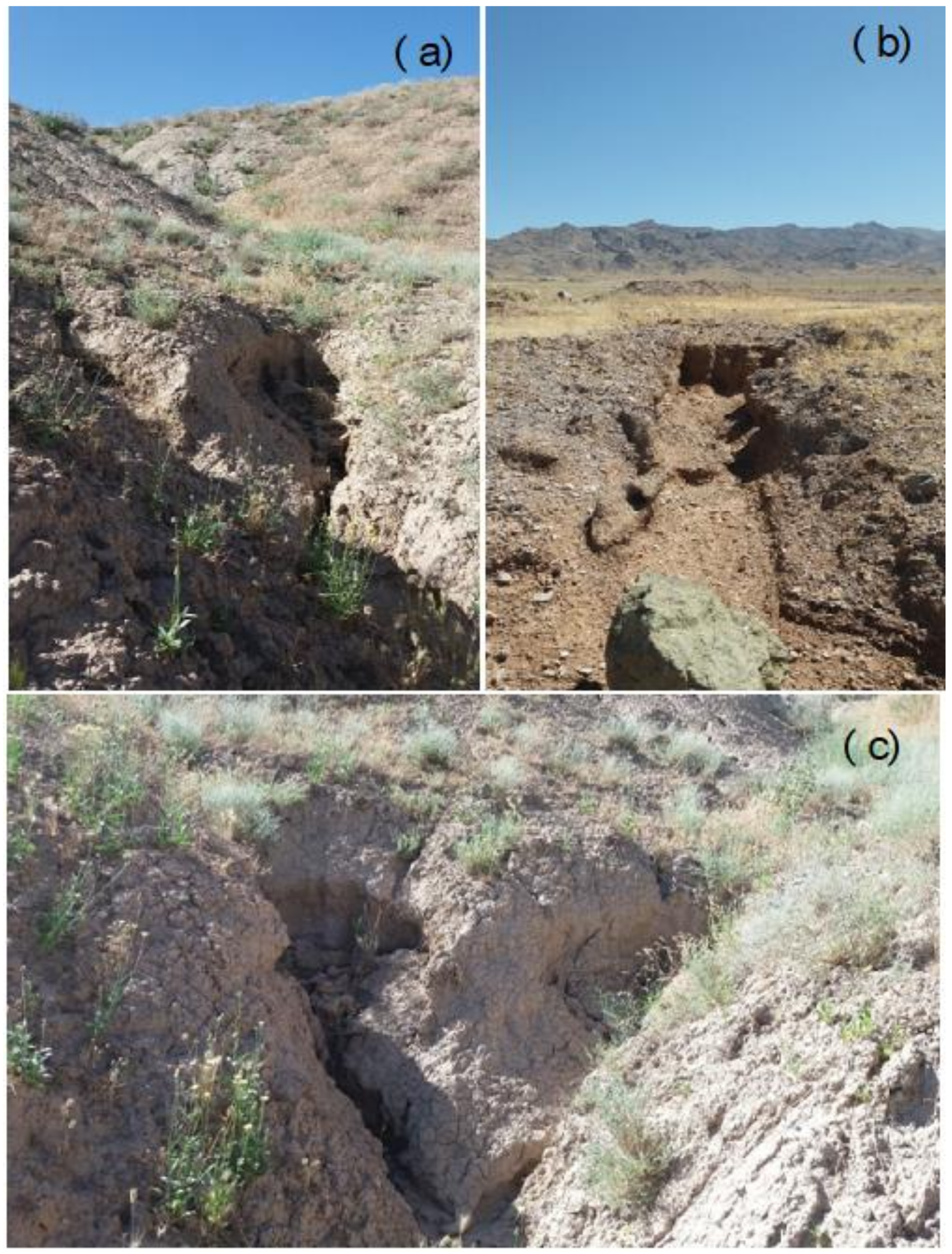
- The gully erosion inventory map and gully erosion causality factors preparations: In the current study, a total of 1115 gully head cut locations were identified using the high-resolution images, field investigation, global positioning system (GPS), and a number of gullies were received from Natural Resources and Watershed Management Organization of the Golestan Province. The 20 environmental factors were considered for the modeling purpose.
- (ii)
- Multi-collinearity analysis among the gully erosion factors using the variance inflation factor (VIF) and tolerance limit was done using SPSS software.
- (iii)
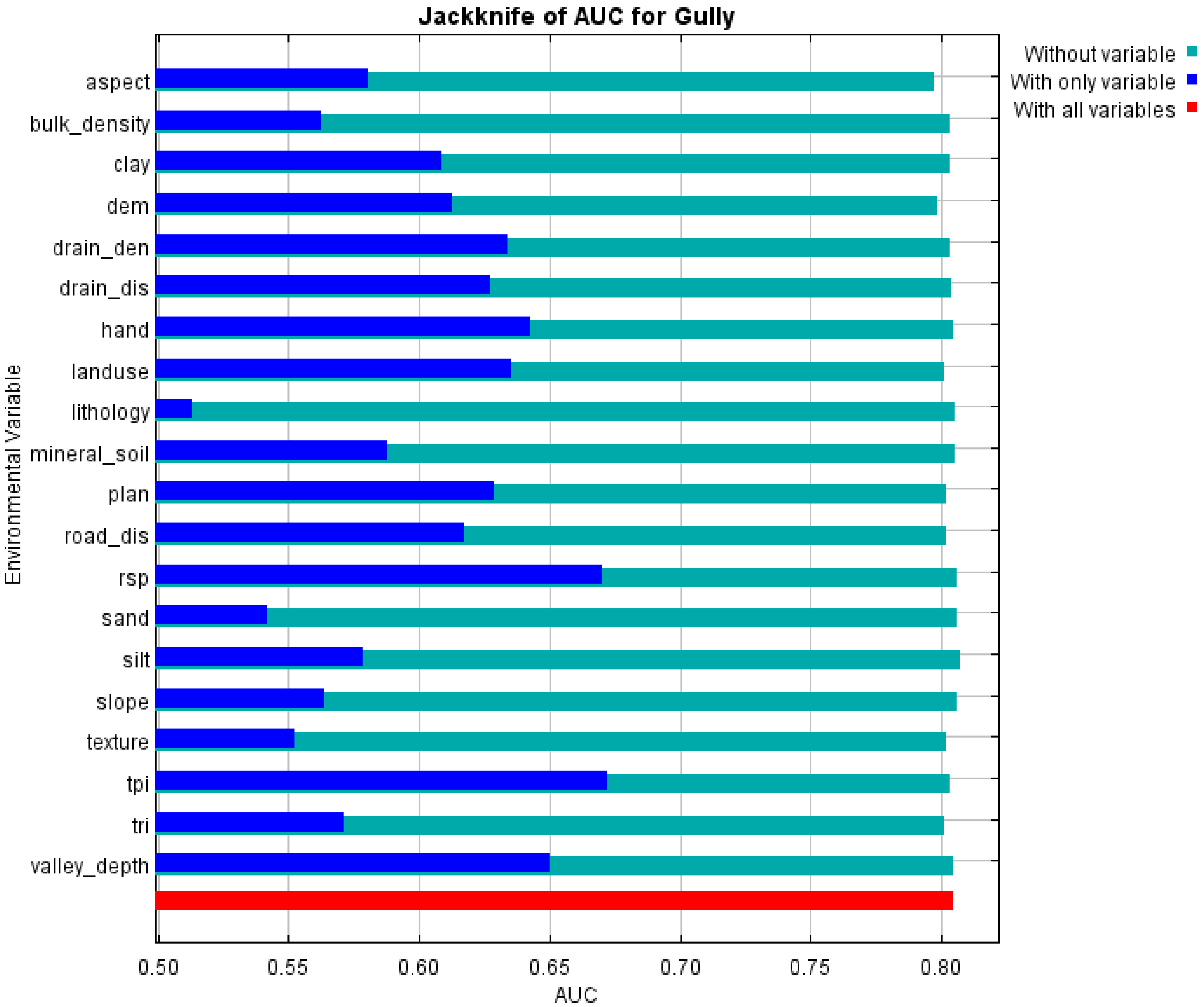
- The significance and effectiveness of factors was carried out using the MaxEnt model (Jackknife test).
- (iv)
- GES maps were prepared using the MaxEnt, ANN, SVM, and GLM models.
- (v)
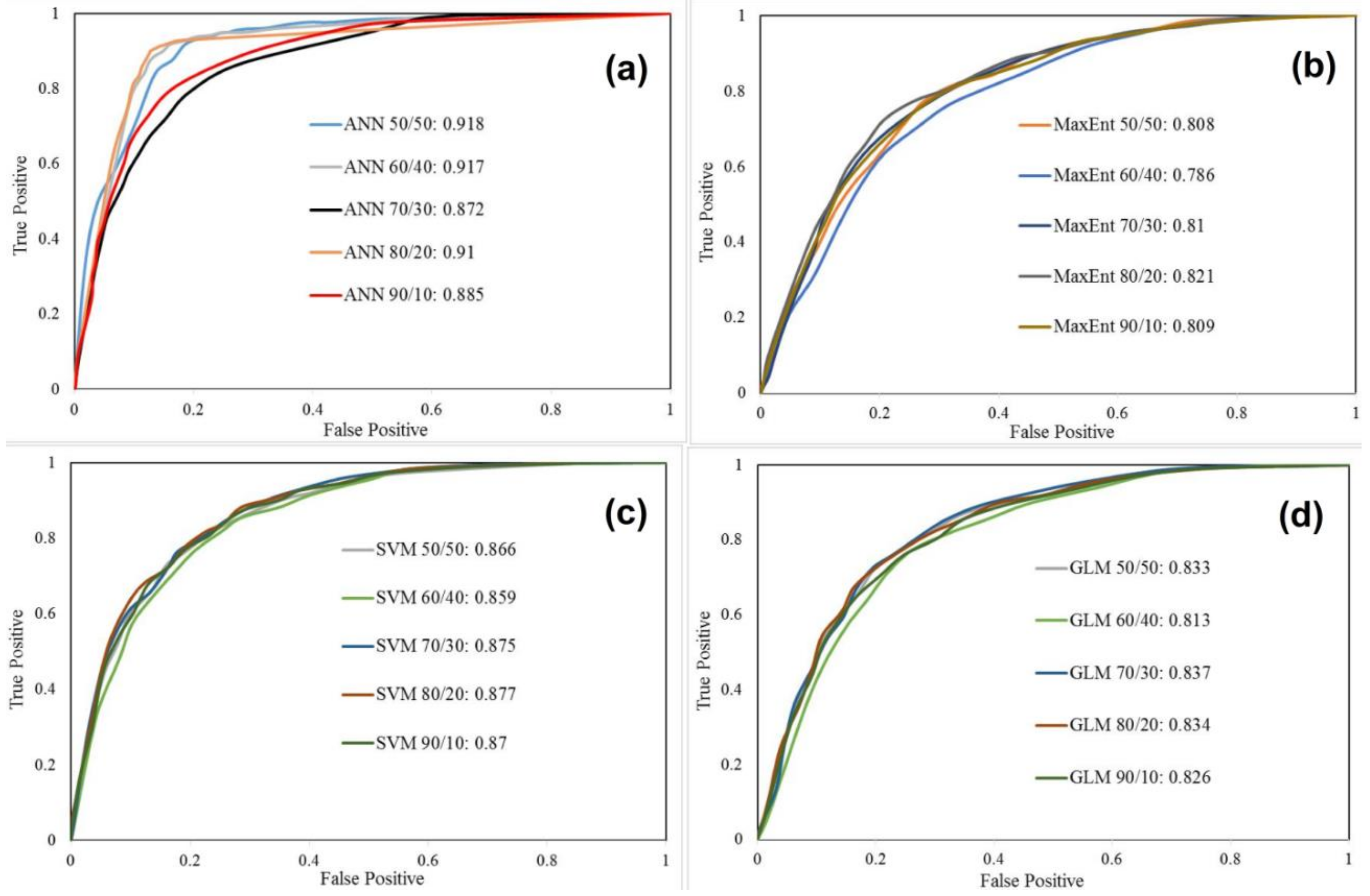
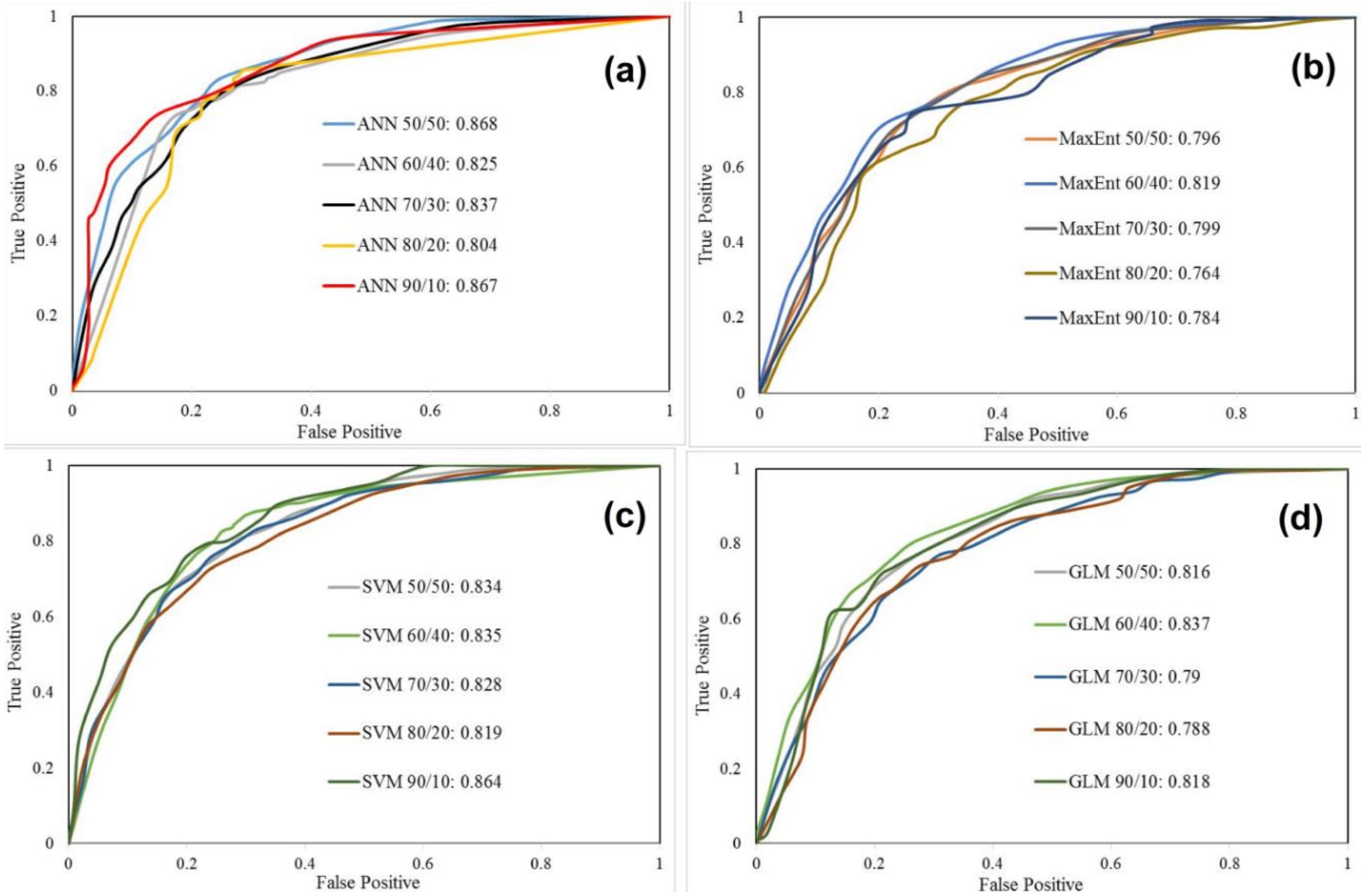
- The GESM model’s performance was validated through the area under receiver operating characteristic curve (AUROC).
2.3. Gully Inventory Map
2.4. Data Preparation
2.5. Multi-Collinearity Assessment
2.6. Methods for Gully Erosion Susceptibility
2.6.1. Artificial Neural Network (ANN)
2.6.2. General Linear Model (GLM)
2.6.3. Maximum Entropy (MaxEnt)
2.6.4. Support Vector Machine (SVM)
2.7. Measuring the Importance of GECFs by the Jackknife Test
2.8. Validation and Accuracy Assessment
3. Results
3.1. Multi-Collinearity Assessment
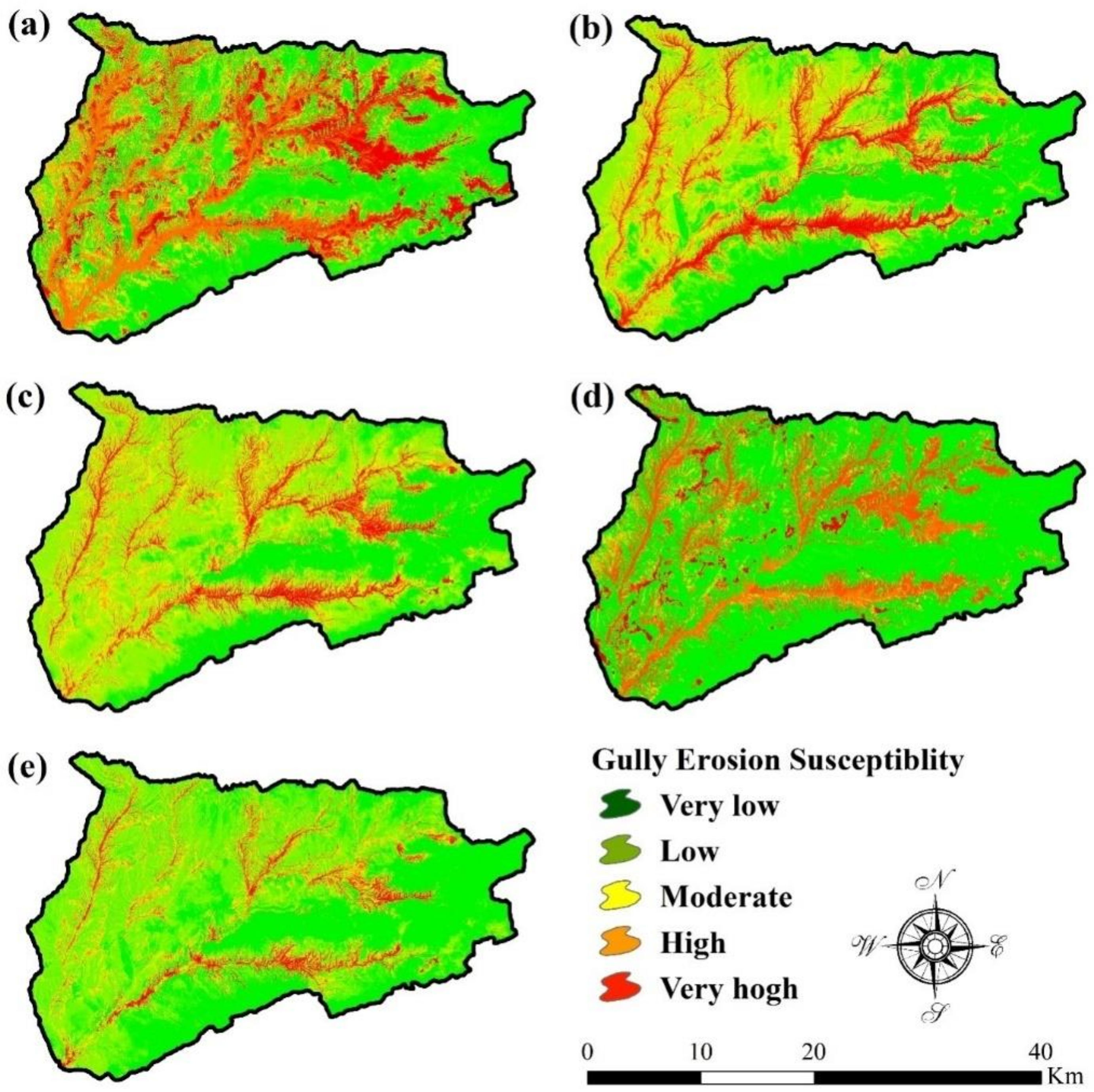
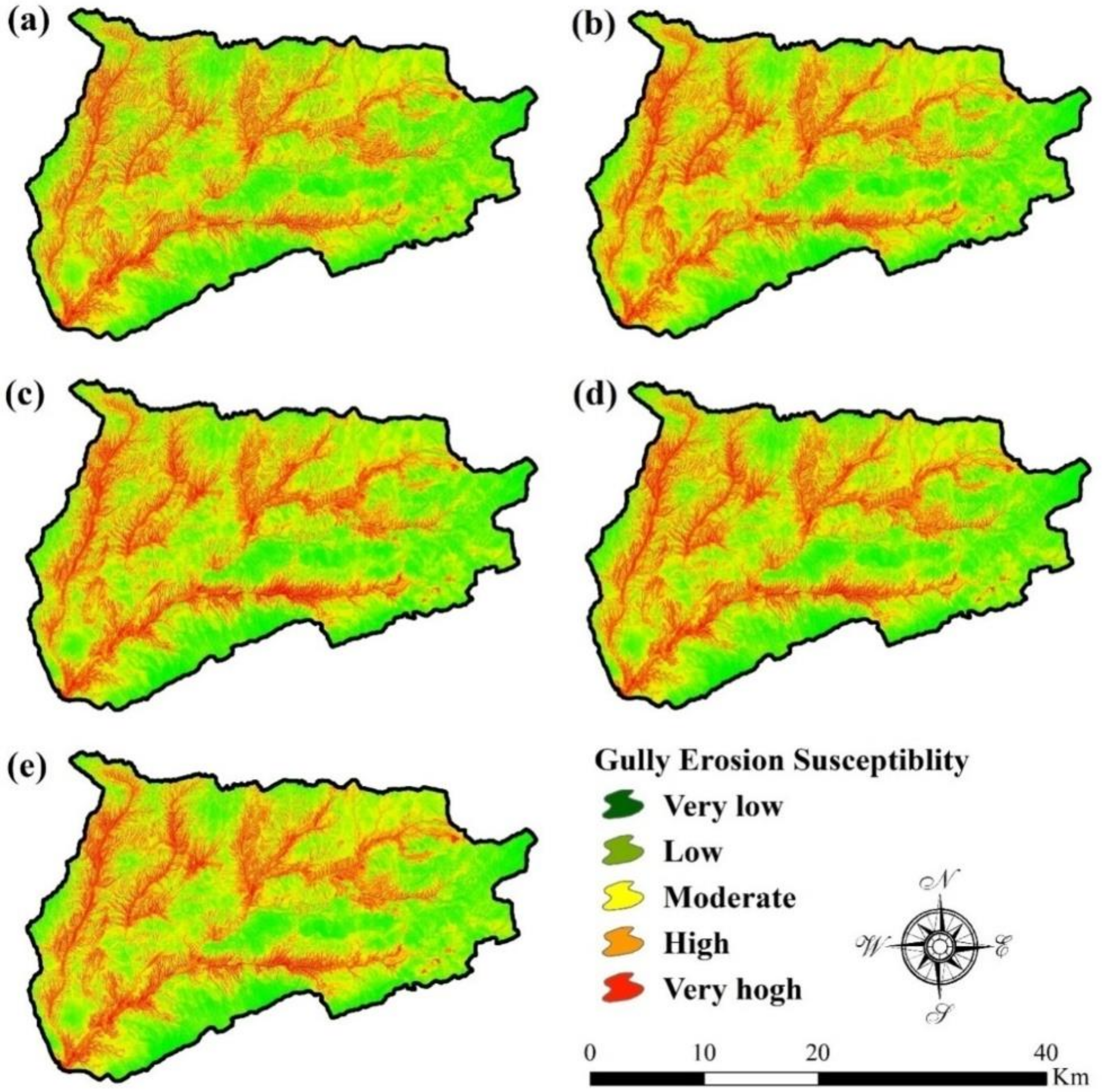
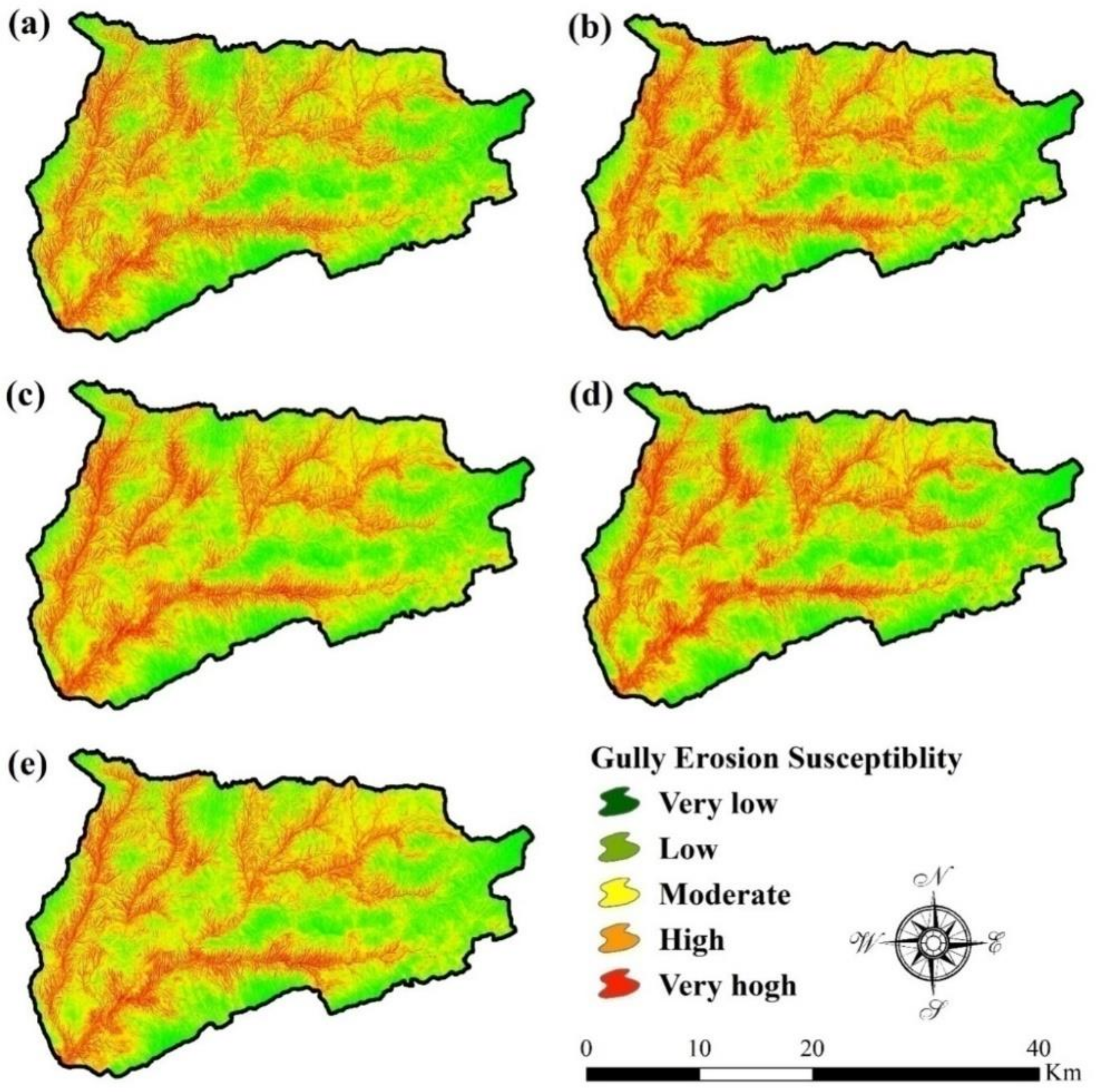
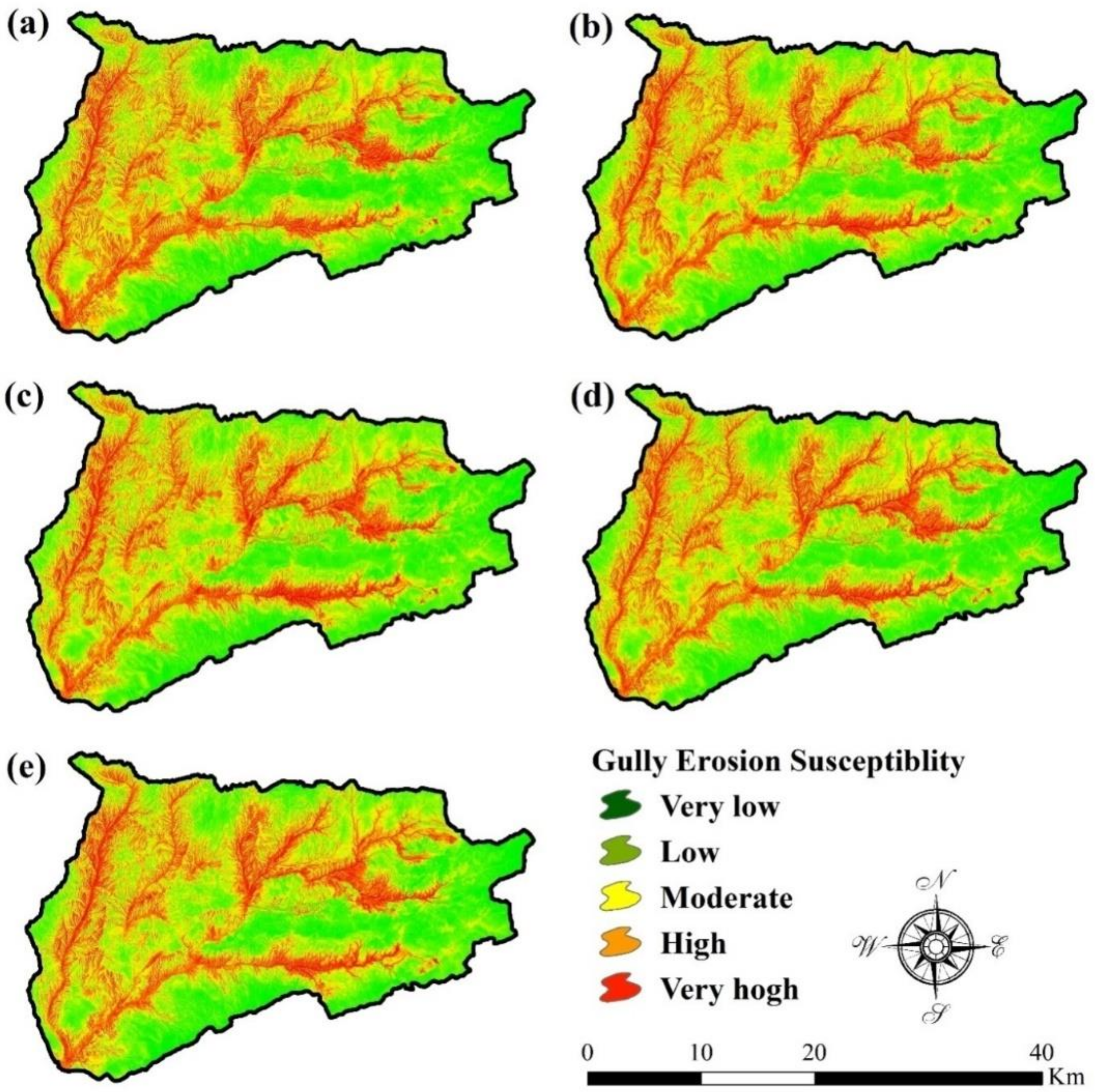
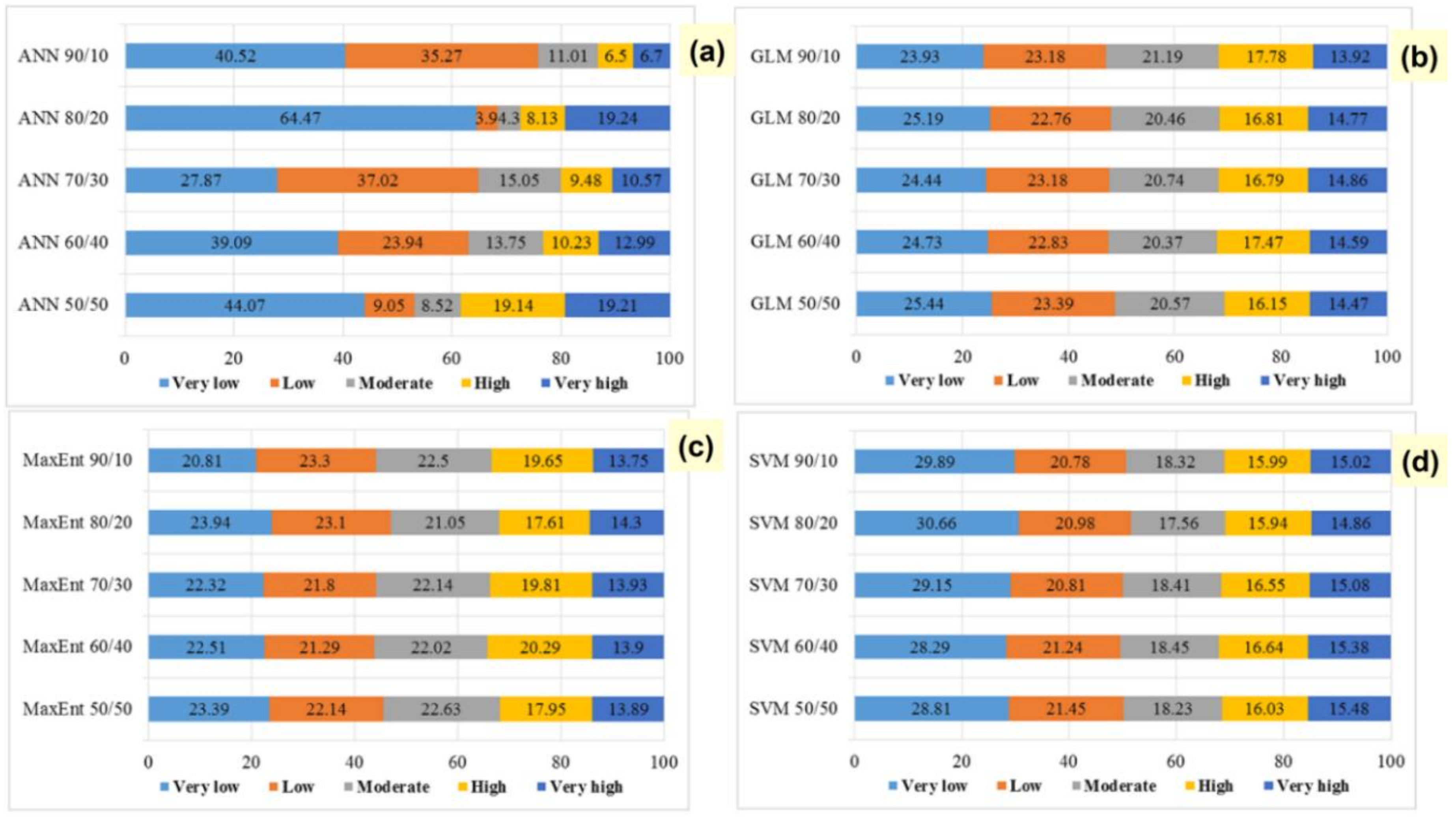
3.2. Gully Erosion Susceptibility Modelling
3.2.1. Gully Erosion Susceptibility Modelling Using Artificial Neural Network (ANN)
3.2.2. Gully Erosion Susceptibility Modelling Using the General Linear Model (GLM)
3.2.3. Gully Erosion Susceptibility Modelling Using Maximum Entropy (MaxEnt)
3.2.4. Gully Erosion Susceptibility Modelling Using Support Vector Machine (SVM)
3.3. Assessing the Importance of the Factors
3.4. Validation of the Models
4. Discussion
Models Prioritization
5. Conclusions
Author Contributions
Funding
Acknowledgments
Conflicts of Interest
References
- Magliulo, P. Assessing the susceptibility to water-induced soil erosion using a geomorphological, bivariate statistics-based approach. Environ. Earth Sci. 2012, 67, 1801–1820. [Google Scholar] [CrossRef]
- Arabameri, A.; Pradhan, B.; Rezaei, K.; Yamani, M.; Pourghasemi, H.R.; Lombardo, L. Spatial modelling of gully erosion using evidential belief function, logistic regression, and a new ensemble of evidential belief function–logistic regression algorithm. Land Degrad. Dev. 2018, 29, 4035–4049. [Google Scholar] [CrossRef]
- Pal, S.C.; Chakrabortty, R. Simulating the impact of climate change on soil erosion in sub-tropical monsoon dominated watershed based on RUSLE, SCS runoff and MIROC5 climatic model. Adv. Space Res. 2019, 64, 352–377. [Google Scholar] [CrossRef]
- Pal, S.C.; Chakrabortty, R. Modeling of water induced surface soil erosion and the potential risk zone prediction in a sub-tropical watershed of Eastern India. Modeling Earth Syst. Environ. 2019, 5, 369–393. [Google Scholar] [CrossRef]
- Pal, S.C.; Shit, M. Application of RUSLE model for soil loss estimation of Jaipanda watershed, West Bengal. Spat. Inf. Res. 2017, 25, 399–409. [Google Scholar] [CrossRef]
- Lal, R. Societal value of soil carbon. J. Soil Water Conserv. 2014, 69, 186A–192A. [Google Scholar] [CrossRef] [Green Version]
- Renard, K.; Yoder, D.; Lightle, D.; Dabney, S. 8 Universal Soil Loss Equation and Revised Universal Soil Loss Equation. In Handbook of Erososion Modelling; Morgan, R.P.C., Nearing, M., Eds.; Wiley: Hoboken, NJ, USA, 2011; Volume 137. [Google Scholar]
- Bobe, B.W. Evaluation of Soil Erosion in the Harerge Region of Ethiopia Using Soil Loss Models, Rainfall Simulation and Field Trials. Ph.D. Thesis, University of Pretoria, Pretoria, South Africa, 2005. [Google Scholar]
- Karimzadeh, H.; Alizadeh, M. Spatial estimation of soil erosion in Iran using RUSLE model. Iran. J. Ecohydrol. 2018. [Google Scholar] [CrossRef]
- Arabameri, A.; Chen, W.; Loche, M.; Zhao, X.; Li, Y.; Lombardo, L.; Cerda, A.; Pradhan, B.; Bui, D.T. Comparison of machine learning models for gully erosion susceptibility mapping. Geosci. Front. 2019. [Google Scholar] [CrossRef]
- Arabameri, A.; Rezaei, K.; Pourghasemi, H.R.; Lee, S.; Yamani, M. GIS-based gully erosion susceptibility mapping: A comparison among three data-driven models and AHP knowledge-based technique. Environ. Earth Sci. 2018, 77, 628. [Google Scholar] [CrossRef]
- Arabameri, A.; Pradhan, B.; Rezaei, K.; Conoscenti, C. Gully erosion susceptibility mapping using GIS-based multi-criteria decision analysis techniques. Catena 2019, 180, 282–297. [Google Scholar] [CrossRef]
- Torri, D.; Poesen, J.; Borselli, L.; Bryan, R.; Rossi, M. Spatial variation of bed roughness in eroding rills and gullies. Catena 2012, 90, 76–86. [Google Scholar] [CrossRef]
- Zhang, X.; Fan, J.; Liu, Q.; Xiong, D. The contribution of gully erosion to total sediment production in a small watershed in Southwest China. Phys. Geogr. 2018, 39, 246–263. [Google Scholar] [CrossRef]
- Rahmati, O.; Tahmasebipour, N.; Haghizadeh, A.; Pourghasemi, H.R.; Feizizadeh, B. Evaluation of different machine learning models for predicting and mapping the susceptibility of gully erosion. Geomorphology 2017, 298, 118–137. [Google Scholar] [CrossRef]
- Nampak, H.; Pradhan, B.; Mojaddadi Rizeei, H.; Park, H. Assessment of land cover and land use change impact on soil loss in a tropical catchment by using multitemporal SPOT-5 satellite images and R evised U niversal Soil L oss E quation model. Land Degrad. Dev. 2018, 29, 3440–3455. [Google Scholar] [CrossRef]
- Saha, A.; Ghosh, M.; Pal, S.C. Understanding the Morphology and Development of a Rill-Gully: An Empirical Study of Khoai Badland, West Bengal, India. In Gully Erosion Studies from India and Surrounding Regions; Springer: Cham, Switzerland, 2020; pp. 147–161. [Google Scholar]
- Imeson, A.; Kwaad, F. Gully types and gully prediction. Geografisch Tijdschrift 1980, 14, 430–441. [Google Scholar]
- Poesen, J. Contribution of gully erosion to sediment production. In Erosion and Sediment Yield: Global and Regional Perspectives, Proceedings of the International Symposium, Exeter, UK, 15–19 July 1996; Walling, D.E., Webb, B., Eds.; IAHS: Wallingford, UK, 1996; p. 251. [Google Scholar]
- Arabameri, A.; Pradhan, B.; Rezaei, K. Spatial prediction of gully erosion using ALOS PALSAR data and ensemble bivariate and data mining models. Geosci. J. 2019, 23, 669–686. [Google Scholar] [CrossRef]
- Kong, B.; Yu, H. Estimation model of soil freeze-thaw erosion in Silingco watershed wetland of northern Tibet. Sci. World J. 2013, 2013, 636521. [Google Scholar] [CrossRef]
- Guerra, A.J.T.; Fullen, M.A.; Jorge, M.d.C.; Bezerra, J.F.R.; Shokr, M.S. Slope processes, mass movement and soil erosion: A review. Pedosphere 2017, 27, 27–41. [Google Scholar] [CrossRef]
- Arabameri, A.; Pradhan, B.; Pourghasemi, H.R.; Rezaei, K.; Kerle, N. Spatial Modelling of Gully Erosion Using GIS and R Programing: A Comparison among Three Data Mining Algorithms. Appl. Sci. 2018, 8, 1369. [Google Scholar] [CrossRef] [Green Version]
- Kirkby, M.; Bracken, L. Gully processes and gully dynamics. Earth Surf. Process. Landf. J. Br. Geomorphol. Res. Group 2009, 34, 1841–1851. [Google Scholar] [CrossRef]
- Daba, S.; Rieger, W.; Strauss, P. Assessment of gully erosion in eastern Ethiopia using photogrammetric techniques. Catena 2003, 50, 273–291. [Google Scholar] [CrossRef]
- Gomez Gutierrez, A.; Schnabel, S.; Felicísimo, Á.M. Modelling the occurrence of gullies in rangelands of southwest Spain. Earth Surf. Process. Landf. J. Br. Geomorphol. Res. Group 2009, 34, 1894–1902. [Google Scholar] [CrossRef]
- Garosi, Y.; Sheklabadi, M.; Conoscenti, C.; Pourghasemi, H.R.; Van Oost, K. Assessing the performance of GIS-based machine learning models with different accuracy measures for determining susceptibility to gully erosion. Sci. Total Environ. 2019, 664, 1117–1132. [Google Scholar] [CrossRef]
- Arabameri, A.; Yamani, M.; Pradhan, B.; Melesse, A.; Shirani, K.; Bui, D.T. Novel ensembles of COPRAS multi-criteria decision-making with logistic regression, boosted regression tree, and random forest for spatial prediction of gully erosion susceptibility. Sci. Total Environ. 2019, 688, 903–916. [Google Scholar] [CrossRef]
- Seber, G.A.; Lee, A.J. Linear Regression Analysis; John Wiley & Sons: Hoboken, NJ, USA, 2012; Volume 329, ISBN 1-118-27442-3. [Google Scholar]
- Arabameri, A.; Pourghasemi, H.R. Spatial modeling of gully erosion using linear and quadratic discriminant analyses in GIS and R. In Spatial Modeling in GIS and R for Earth and Environmental Sciences; Elsevier: Amsterdam, The Netherlands, 2019; pp. 299–321. [Google Scholar]
- Arabameri, A.; Pourghasemi, H.R.; Yamani, M. Applying different scenarios for landslide spatial modeling using computational intelligence methods. Environ. Earth Sci. 2017, 76, 832. [Google Scholar] [CrossRef]
- Arabameri, A.; Lee, S.; Tiefenbacher, J.P.; Ngo, P.T.T. Novel Ensemble of MCDM-Artificial Intelligence Techniques for Groundwater-Potential Mapping in Arid and Semi-Arid Regions (Iran). Remote Sens. 2020, 12, 490. [Google Scholar] [CrossRef] [Green Version]
- Kujawski, E. Multi-Criteria Decision Analysis: Limitations, Pitfalls, and Practical Difficulties. 2003; Lawrence Berkeley National Laboratory: Berkley, CA, USA, 2007.
- Reilly, T. Making Hard Decisions with Decision Tools; Duxbury Thomson Learning: Boston, MA, USA, 2001; ISBN 0-534-36597-3. [Google Scholar]
- Conforti, M.; Aucelli, P.P.C.; Robustelli, G.; Scarciglia, F. Geomorphology and GIS analysis for mapping gully erosion susceptibility in the Turbolo stream catchment (Northern Calabria, Italy). Nat. Hazards 2011, 56, 881–898. [Google Scholar] [CrossRef]
- Rahmati, O.; Tahmasebipour, N.; Haghizadeh, A.; Pourghasemi, H.R.; Feizizadeh, B. Evaluating the influence of geo-environmental factors on gully erosion in a semi-arid region of Iran: An integrated framework. Sci. Total Environ. 2017, 579, 913–927. [Google Scholar] [CrossRef]
- Hosseinalizadeh, M.; Kariminejad, N.; Rahmati, O.; Keesstra, S.; Alinejad, M.; Mohammadian Behbahani, A. How can statistical and artificial intelligence approaches predict piping erosion susceptibility? Sci. Total Environ. 2019, 646, 1554–1566. [Google Scholar] [CrossRef]
- Zabihi, M.; Mirchooli, F.; Motevalli, A.; Khaledi Darvishan, A.; Pourghasemi, H.R.; Zakeri, M.A.; Sadighi, F. Spatial modelling of gully erosion in Mazandaran Province, northern Iran. Catena 2018, 161, 1–13. [Google Scholar] [CrossRef]
- Azareh, A.; Rahmati, O.; Rafiei-Sardooi, E.; Sankey, J.B.; Lee, S.; Shahabi, H.; Ahmad, B.B. Modelling gully-erosion susceptibility in a semi-arid region, Iran: Investigation of applicability of certainty factor and maximum entropy models. Sci. Total Environ. 2019, 655, 684–696. [Google Scholar] [CrossRef] [PubMed]
- Rahmati, O.; Haghizadeh, A.; Pourghasemi, H.R.; Noormohamadi, F. Gully erosion susceptibility mapping: The role of GIS-based bivariate statistical models and their comparison. Nat. Hazards 2016, 82, 1231–1258. [Google Scholar] [CrossRef]
- Arabameri, A.; Chen, W.; Lombardo, L.; Blaschke, T.; Tien Bui, D. Hybrid Computational Intelligence Models for Improvement Gully Erosion Assessment. Remote Sens. 2020, 12, 140. [Google Scholar] [CrossRef] [Green Version]
- Roy, P.; Chakrabortty, R.; Chowdhuri, I.; Malik, S.; Das, B.; Pal, S.C. Development of Different Machine Learning Ensemble Classifier for Gully Erosion Susceptibility in Gandheswari Watershed of West Bengal, India. In Machine Learning for Intelligent Decision Science; Rout, J.K., Rout, M., Das, H., Eds.; Algorithms for Intelligent Systems; Springer: Singapore, 2020; pp. 1–26. ISBN 9789811536885. [Google Scholar]
- Pourghasemi, H.R.; Yousefi, S.; Kornejady, A.; Cerdà, A. Performance assessment of individual and ensemble data-mining techniques for gully erosion modeling. Sci. Total Environ. 2017, 609, 764–775. [Google Scholar] [CrossRef] [Green Version]
- Amiri, M.; Pourghasemi, H.R.; Ghanbarian, G.A.; Afzali, S.F. Assessment of the importance of gully erosion effective factors using Boruta algorithm and its spatial modeling and mapping using three machine learning algorithms. Geoderma 2019, 340, 55–69. [Google Scholar] [CrossRef]
- Geissen, V.; Kampichler, C.; López-de Llergo-Juárez, J.J.; Galindo-Acántara, A. Superficial and subterranean soil erosion in Tabasco, tropical Mexico: Development of a decision tree modeling approach. Geoderma 2007, 139, 277–287. [Google Scholar] [CrossRef]
- Angileri, S.E.; Conoscenti, C.; Hochschild, V.; Märker, M.; Rotigliano, E.; Agnesi, V. Water erosion susceptibility mapping by applying Stochastic Gradient Treeboost to the Imera Meridionale River Basin (Sicily, Italy). Geomorphology 2016, 262, 61–76. [Google Scholar] [CrossRef]
- Hosseinalizadeh, M.; Kariminejad, N.; Chen, W.; Pourghasemi, H.R.; Alinejad, M.; Mohammadian Behbahani, A.; Tiefenbacher, J.P. Gully headcut susceptibility modeling using functional trees, naïve Bayes tree, and random forest models. Geoderma 2019, 342, 1–11. [Google Scholar] [CrossRef]
- Hosseinalizadeh, M.; Kariminejad, N.; Chen, W.; Pourghasemi, H.R.; Alinejad, M.; Mohammadian Behbahani, A.; Tiefenbacher, J.P. Spatial modelling of gully headcuts using UAV data and four best-first decision classifier ensembles (BFTree, Bag-BFTree, RS-BFTree, and RF-BFTree). Geomorphology 2019, 329, 184–193. [Google Scholar] [CrossRef]
- Gayen, A.; Pourghasemi, H.R. Spatial Modeling of Gully Erosion. In Spatial Modeling in GIS and R for Earth and Environmental Sciences; Elsevier: Amsterdam, The Netherlands, 2019; pp. 653–669. ISBN 978-0-12-815226-3. [Google Scholar]
- Saha, S.; Roy, J.; Arabameri, A.; Blaschke, T.; Tien Bui, D. Machine Learning-Based Gully Erosion Susceptibility Mapping: A Case Study of Eastern India. Sensors 2020, 20, 1313. [Google Scholar] [CrossRef] [Green Version]
- Varshney, K.R.; Alemzadeh, H. On the safety of machine learning: Cyber-physical systems, decision sciences, and data products. Big Data 2017, 5, 246–255. [Google Scholar] [CrossRef] [PubMed]
- Arabameri, A.; Asadi Nalivan, O.; Saha, S.; Roy, J.; Pradhan, B.; Tiefenbacher, J.P.; Thi Ngo, P.T. Novel Ensemble Approaches of Machine Learning Techniques in Modeling the Gully Erosion Susceptibility. Remote Sens. 2020, 12, 1890. [Google Scholar] [CrossRef]
- Javidan, N.; Kavian, A.; Pourghasemi, H.R.; Conoscenti, C.; Jafarian, Z. Data Mining Technique (Maximum Entropy Model) for Mapping Gully Erosion Susceptibility in the Gorganrood Watershed, Iran. In Gully Erosion Studies from India and Surrounding Regions; Shit, P.K., Pourghasemi, H.R., Bhunia, G.S., Eds.; Advances in Science, Technology & Innovation; Springer International Publishing: Cham, Switzerland, 2020; pp. 427–448. ISBN 978-3-030-23242-9. [Google Scholar]
- Garosi, Y.; Sheklabadi, M.; Pourghasemi, H.R.; Besalatpour, A.A.; Conoscenti, C.; Van Oost, K. Comparison of differences in resolution and sources of controlling factors for gully erosion susceptibility mapping. Geoderma 2018, 330, 65–78. [Google Scholar] [CrossRef]
- Pourghasemi, H.R.; Rossi, M. Landslide susceptibility modeling in a landslide prone area in Mazandarn Province, north of Iran: A comparison between GLM, GAM, MARS, and M-AHP methods. Theor. Appl. Clim. 2017, 130, 609–633. [Google Scholar] [CrossRef]
- De Reu, J.; Bourgeois, J.; Bats, M.; Zwertvaegher, A.; Gelorini, V.; De Smedt, P.; Chu, W.; Antrop, M.; De Maeyer, P.; Finke, P.; et al. Application of the topographic position index to heterogeneous landscapes. Geomorphology 2013, 186, 39–49. [Google Scholar] [CrossRef]
- Heerdegen, R.G.; Beran, M.A. Quantifying source areas through land surface curvature and shape. J. Hydrol. 1982, 57, 359–373. [Google Scholar] [CrossRef]
- Zevenbergen, L.W.; Thorne, C.R. Quantitative analysis of land surface topography. Earth Surf. Process. Landf. 1987, 12, 47–56. [Google Scholar] [CrossRef]
- Nobre, A.D.; Cuartas, L.A.; Hodnett, M.; Rennó, C.D.; Rodrigues, G.; Silveira, A.; Waterloo, M.; Saleska, S. Height Above the Nearest Drainage—A hydrologically relevant new terrain model. J. Hydrol. 2011, 404, 13–29. [Google Scholar] [CrossRef] [Green Version]
- Horton, R.E. Erosional development of streams and their drainage basins; hydrophysical approach to quantitative morphology. Geol. Soc Am. Bull. 1945, 56, 275. [Google Scholar] [CrossRef] [Green Version]
- Trigila, A.; Iadanza, C.; Esposito, C.; Scarascia-Mugnozza, G. Comparison of Logistic Regression and Random Forests techniques for shallow landslide susceptibility assessment in Giampilieri (NE Sicily, Italy). Geomorphology 2015, 249, 119–136. [Google Scholar] [CrossRef]
- Du, G.; Zhang, Y.; Iqbal, J.; Yang, Z.; Yao, X. Landslide susceptibility mapping using an integrated model of information value method and logistic regression in the Bailongjiang watershed, Gansu Province, China. J. Mt. Sci. 2017, 14, 249–268. [Google Scholar] [CrossRef]
- Amidon, G.E.; Secreast, P.J.; Mudie, D. Particle, Powder, and Compact Characterization. In Developing Solid Oral Dosage Forms; Elsevier: Amsterdam, The Netherlands, 2009; pp. 163–186. ISBN 978-0-444-53242-8. [Google Scholar]
- Rahmati, O.; Moghaddam, D.D.; Moosavi, V.; Kalantari, Z.; Samadi, M.; Lee, S.; Tien Bui, D. An Automated Python Language-Based Tool for Creating Absence Samples in Groundwater Potential Mapping. Remote Sens. 2019, 11, 1375. [Google Scholar] [CrossRef] [Green Version]
- Gallant, J.C.; Austin, J.M. Derivation of terrain covariates for digital soil mapping in Australia. Soil Res. 2015, 53, 895. [Google Scholar] [CrossRef]
- Conoscenti, C.; Agnesi, V.; Angileri, S.; Cappadonia, C.; Rotigliano, E.; Märker, M. A GIS-based approach for gully erosion susceptibility modelling: A test in Sicily, Italy. Environ. Earth Sci. 2013, 70, 1179–1195. [Google Scholar] [CrossRef]
- Ahmad, R. Landslides Processes, Prediction, and Land Use: Water Resources Monograph 18—By Roy C. Sidle and Hirotaka Ochiai. Nat. Resour. Forum 2007, 31, 322–323. [Google Scholar] [CrossRef]
- Chakrabortty, R.; Pal, S.C.; Sahana, M.; Mondal, A.; Dou, J.; Pham, B.T.; Yunus, A.P. Soil erosion potential hotspot zone identification using machine learning and statistical approaches in eastern India. Nat. Hazards 2020. [Google Scholar] [CrossRef]
- Garousi-Nejad, I.; Tarboton, D.G.; Aboutalebi, M.; Torres-Rua, A.F. Terrain Analysis Enhancements to the Height Above Nearest Drainage Flood Inundation Mapping Method. Water Resour. Res. 2019, 55, 7983–8009. [Google Scholar] [CrossRef]
- Horton, R.E. Drainage-basin characteristics. Trans. AGU 1932, 13, 350. [Google Scholar] [CrossRef]
- Conoscenti, C.; Angileri, S.; Cappadonia, C.; Rotigliano, E.; Agnesi, V.; Märker, M. Gully erosion susceptibility assessment by means of GIS-based logistic regression: A case of Sicily (Italy). Geomorphology 2014, 204, 399–411. [Google Scholar] [CrossRef] [Green Version]
- Althuwaynee, O.F.; Pradhan, B.; Park, H.-J.; Lee, J.H. A novel ensemble bivariate statistical evidential belief function with knowledge-based analytical hierarchy process and multivariate statistical logistic regression for landslide susceptibility mapping. Catena 2014, 114, 21–36. [Google Scholar] [CrossRef]
- Davoudi Moghaddam, D.; Rahmati, O.; Haghizadeh, A.; Kalantari, Z. A Modeling Comparison of Groundwater Potential Mapping in a Mountain Bedrock Aquifer: QUEST, GARP, and RF Models. Water 2020, 12, 679. [Google Scholar] [CrossRef] [Green Version]
- Pourghasemi, H.R.; Kerle, N. Random forests and evidential belief function-based landslide susceptibility assessment in Western Mazandaran Province, Iran. Environ. Earth Sci. 2016, 75, 185. [Google Scholar] [CrossRef]
- El Maaoui, M.A.; Sfar Felfoul, M.; Boussema, M.R.; Snane, M.H. Sediment yield from irregularly shaped gullies located on the Fortuna lithologic formation in semi-arid area of Tunisia. Catena 2012, 93, 97–104. [Google Scholar] [CrossRef]
- Wang, G.; Chen, X.; Chen, W. Spatial Prediction of Landslide Susceptibility Based on GIS and Discriminant Functions. IJGI 2020, 9, 144. [Google Scholar] [CrossRef] [Green Version]
- Chen, W.; Sun, Z.; Han, J. Landslide Susceptibility Modeling Using Integrated Ensemble Weights of Evidence with Logistic Regression and Random Forest Models. Appl. Sci. 2019, 9, 171. [Google Scholar] [CrossRef] [Green Version]
- Haykin, S. Neural Networks: A Comprehensive Foundation, 2nd ed.; Prentice Hall: Englewood Cliffs, NJ, USA, 1999. [Google Scholar]
- Cherkassky, V.; Krasnopolsky, V.; Solomatine, D.P.; Valdes, J. Computational intelligence in earth sciences and environmental applications: Issues and challenges. Neural Netw. 2006, 19, 113–121. [Google Scholar] [CrossRef]
- Kosko, B. Neural Networks and Fuzzy Systems: A Dynamical Systems Approach to Machine Intelligence; Prentice Hall: New York, NY, USA, 1992. [Google Scholar]
- Mandal, S.; Mondal, S. Statistical Approaches for Landslide Susceptibility Assessment and Prediction; Springer: Cham, Switzerland, 2019; ISBN 978-3-319-93897-4. [Google Scholar]
- Falaschi, F.; Giacomelli, F.; Federici, P.R.; Puccinelli, A.; D’Amato Avanzi, G.; Pochini, A.; Ribolini, A. Logistic regression versus artificial neural networks: Landslide susceptibility evaluation in a sample area of the Serchio River valley, Italy. Nat. Hazards 2009, 50, 551–569. [Google Scholar] [CrossRef]
- Gong, P.; Pu, R.; Chen, J. Elevation and forest-cover data using neural networks. Photogramm. Eng. Remote Sens. 1996, 62, 1249–1260. [Google Scholar]
- Hagan, M.T.; Demuth, H.B.; Beale, M.H.; De Jesus, O. Neural Network Design, 2nd ed.; Amazon Fulfillment Poland Sp. z o.o: Wrocław, Poland, 1996; ISBN 978-0-9717321-1-7. [Google Scholar]
- Lucà, F.; Conforti, M.; Robustelli, G. Comparison of GIS-based gullying susceptibility mapping using bivariate and multivariate statistics: Northern Calabria, South Italy. Geomorphology 2011, 134, 297–308. [Google Scholar] [CrossRef]
- McCullagh, P.; Nelder, J. Generalized Linear Models, 2nd ed.; Standard Book on Generalized Linear Models; Chapman and Hall: London, UK, 1989. [Google Scholar]
- Nelder, J.A.; Wedderburn, R.W. Generalized linear models. J. R. Stat. Soc. Ser. A (General) 1972, 135, 370–384. [Google Scholar] [CrossRef]
- Vorpahl, P.; Elsenbeer, H.; Märker, M.; Schröder, B. How can statistical models help to determine driving factors of landslides? Ecol. Model. 2012, 239, 27–39. [Google Scholar] [CrossRef]
- Maunder, M.N.; Punt, A.E. Standardizing catch and effort data: A review of recent approaches. Fish. Res. 2004, 70, 141–159. [Google Scholar] [CrossRef]
- Naghibi, S.A.; Pourghasemi, H.R. A comparative assessment between three machine learning models and their performance comparison by bivariate and multivariate statistical methods in groundwater potential mapping. Water Resour. Manag. 2015, 29, 5217–5236. [Google Scholar] [CrossRef]
- Bernknopf, R.L.; Campbell, R.H.; Brookshire, D.S.; Shapiro, C.D. A Probabilistic Approach to Landslide Hazard Mapping in Cincinnati, Ohio, with Applications for Economic Evaluation. Environ. Eng. Geosci. 1988, xxv, 39–56. [Google Scholar] [CrossRef]
- Woodbury, A.; Render, F.; Ulrych, T. Practical probabilistic ground-water modeling. Ground Water 1995, 33, 532–539. [Google Scholar] [CrossRef]
- Phillips, S.J.; Anderson, R.P.; Schapire, R.E. Maximum entropy modeling of species geographic distributions. Ecol. Model. 2006, 190, 231–259. [Google Scholar] [CrossRef] [Green Version]
- Phillips, S.J.; Dudík, M. Modeling of species distributions with Maxent: New extensions and a comprehensive evaluation. Ecography 2008, 31, 161–175. [Google Scholar] [CrossRef]
- Reddy, S.; Dávalos, L.M. Geographical sampling bias and its implications for conservation priorities in Africa. J. Biogeogr. 2003, 30, 1719–1727. [Google Scholar] [CrossRef]
- Kornejady, A.; Ownegh, M.; Bahremand, A. Landslide susceptibility assessment using maximum entropy model with two different data sampling methods. Catena 2017, 152, 144–162. [Google Scholar] [CrossRef]
- Phillips, S.J.; Dudík, M.; Elith, J.; Graham, C.H.; Lehmann, A.; Leathwick, J.; Ferrier, S. Sample selection bias and presence-only distribution models: Implications for background and pseudo-absence data. Ecol. Appl. 2009, 19, 181–197. [Google Scholar] [CrossRef] [Green Version]
- Elith, J.; Phillips, S.J.; Hastie, T.; Dudík, M.; Chee, Y.E.; Yates, C.J. A statistical explanation of MaxEnt for ecologists. Divers. Distrib. 2011, 17, 43–57. [Google Scholar] [CrossRef]
- Vapnik, V.; Guyon, I.; Hastie, T. Support vector machines. Mach. Learn 1995, 20, 273–297. [Google Scholar]
- Cristianini, N.; Shawe-Taylor, J. An Introduction to Support Vector Machines and Other Kernel-Based Learning Methods; Cambridge University Press: Cambridge, UK, 2000; ISBN 0-521-78019-5. [Google Scholar]
- Joachims, T. Text Categorization with Support Vector Machines: Learning with Many Relevant Features; Springer: Cham, Switzerland, 1998; pp. 137–142. [Google Scholar]
- Pradhan, B. A comparative study on the predictive ability of the decision tree, support vector machine and neuro-fuzzy models in landslide susceptibility mapping using GIS. Comput. Geosci. 2013, 51, 350–365. [Google Scholar] [CrossRef]
- Lee, S.; Hong, S.-M.; Jung, H.-S. A support vector machine for landslide susceptibility mapping in Gangwon Province, Korea. Sustainability 2017, 9, 48. [Google Scholar] [CrossRef] [Green Version]
- Yao, X.; Tham, L.; Dai, F. Landslide susceptibility mapping based on support vector machine: A case study on natural slopes of Hong Kong, China. Geomorphology 2008, 101, 572–582. [Google Scholar] [CrossRef]
- Yilmaz, I. Comparison of landslide susceptibility mapping methodologies for Koyulhisar, Turkey: Conditional probability, logistic regression, artificial neural networks, and support vector machine. Environ. Earth Sci. 2010, 61, 821–836. [Google Scholar] [CrossRef]
- Xu, C.; Xu, X.; Dai, F.; Saraf, A.K. Comparison of different models for susceptibility mapping of earthquake triggered landslides related with the 2008 Wenchuan earthquake in China. Comput. Geosci. 2012, 46, 317–329. [Google Scholar] [CrossRef]
- Hastie, T.; Tibshirani, R.; Friedman, J. The Elements of Statistical Learning: Data Mining, Inference, and Prediction; Springer Science & Business Media: Cham, Switzerland, 2009; ISBN 0-387-84858-4. [Google Scholar]
- Efron, B. The Jackknife, the Bootstrap and Other Resampling Plans; Society for Industrial and Applied Mathematics: Philadelphia, PA, USA, 1982; ISBN 978-0-89871-179-0. [Google Scholar]
- Bandos, A.I.; Guo, B.; Gur, D. Jackknife variance of the partial area under the empirical receiver operating characteristic curve. Stat. Methods Med. Res. 2017, 26, 528–541. [Google Scholar] [CrossRef] [Green Version]
- Convertino, M.; Troccoli, A.; Catani, F. Detecting fingerprints of landslide drivers: A MaxEnt model: Fingerprints of landslide drivers. J. Geophys. Res. Earth Surf. 2013, 118, 1367–1386. [Google Scholar] [CrossRef] [Green Version]
- Park, N.-W. Using maximum entropy modeling for landslide susceptibility mapping with multiple geoenvironmental data sets. Environ. Earth Sci. 2015, 73, 937–949. [Google Scholar] [CrossRef]
- Arabameri, A.; Cerda, A.; Rodrigo-Comino, J.; Pradhan, B.; Sohrabi, M.; Blaschke, T.; Tien Bui, D. Proposing a Novel Predictive Technique for Gully Erosion Susceptibility Mapping in Arid and Semi-arid Regions (Iran). Remote Sens. 2019, 11, 2577. [Google Scholar] [CrossRef] [Green Version]
- Roy, J.; Saha, S.; Arabameri, A.; Blaschke, T.; Bui, D.T. A Novel Ensemble Approach for Landslide Susceptibility Mapping (LSM) in Darjeeling and Kalimpong Districts, West Bengal, India. Remote Sens. 2019, 11, 2866. [Google Scholar] [CrossRef] [Green Version]
- Frattini, P.; Crosta, G.; Carrara, A. Techniques for evaluating the performance of landslide susceptibility models. Eng. Geol. 2010, 111, 62–72. [Google Scholar] [CrossRef]
- Pham, B.T.; Prakash, I. Evaluation and comparison of LogitBoost Ensemble, Fisher’s Linear Discriminant Analysis, logistic regression and support vector machines methods for landslide susceptibility mapping. Geocarto Int. 2019, 34, 316–333. [Google Scholar] [CrossRef]
- Fressard, M.; Thiery, Y.; Maquaire, O. Which data for quantitative landslide susceptibility mapping at operational scale? Case study of the Pays d’Auge plateau hillslopes (Normandy, France). Nat. Hazards Earth Syst. Sci. 2014, 14, 569–588. [Google Scholar] [CrossRef] [Green Version]
- Pourghasemi, H.R.; Sadhasivam, N.; Kariminejad, N.; Collins, A.L. Gully erosion spatial modelling: Role of machine learning algorithms in selection of the best controlling factors and modelling process. Geosci. Front. 2020. [Google Scholar] [CrossRef]
- Arabameri, A.; Cerda, A.; Pradhan, B.; Tiefenbacher, J.P.; Lombardo, L.; Bui, D.T. A methodological comparison of head-cut based gully erosion susceptibility models: Combined use of statistical and artificial intelligence. Geomorphology 2020, 359, 107136. [Google Scholar] [CrossRef]
- Conway, S.J.; Decaulne, A.; Balme, M.R.; Murray, J.B.; Towner, M.C. A new approach to estimating hazard posed by debris flows in the Westfjords of Iceland. Geomorphology 2010, 114, 556–572. [Google Scholar] [CrossRef] [Green Version]
- Razavi-Termeh, S.V.; Sadeghi-Niaraki, A.; Choi, S.-M. Gully erosion susceptibility mapping using artificial intelligence and statistical models. Geomat. Nat. Hazards Risk 2020, 11, 821–845. [Google Scholar] [CrossRef]
- Arabameri, A.; Pradhan, B.; Lombardo, L. Comparative assessment using boosted regression trees, binary logistic regression, frequency ratio and numerical risk factor for gully erosion susceptibility modelling. Catena 2019, 183, 104223. [Google Scholar] [CrossRef]
- Avand, M.; Janizadeh, S.; Naghibi, S.A.; Pourghasemi, H.R.; Khosrobeigi Bozchaloei, S.; Blaschke, T. A Comparative Assessment of Random Forest and k-Nearest Neighbor Classifiers for Gully Erosion Susceptibility Mapping. Water 2019, 11, 2076. [Google Scholar] [CrossRef] [Green Version]
- Chauchard, F.; Cogdill, R.; Roussel, S.; Roger, J.M.; Bellon-Maurel, V. Application of LS-SVM to non-linear phenomena in NIR spectroscopy: Development of a robust and portable sensor for acidity prediction in grapes. Chemom. Intell. Lab. Syst. 2004, 71, 141–150. [Google Scholar] [CrossRef] [Green Version]
- Raj Kiran, N.; Ravi, V. Software reliability prediction by soft computing techniques. J. Syst. Softw. 2008, 81, 576–583. [Google Scholar] [CrossRef]
- Yuan, H.; Yang, G.; Li, C.; Wang, Y.; Liu, J.; Yu, H.; Feng, H.; Xu, B.; Zhao, X.; Yang, X. Retrieving Soybean Leaf Area Index from Unmanned Aerial Vehicle Hyperspectral Remote Sensing: Analysis of RF, ANN, and SVM Regression Models. Remote Sens. 2017, 9, 309. [Google Scholar] [CrossRef] [Green Version]
- Fogno Fotso, H.R.; Aloyem Kazé, C.V.; Kenmoe, G.D. Optimal Input Variables Disposition of Artificial Neural Networks Models for Enhancing Time Series Forecasting Accuracy. Appl. Artif. Intell. 2020, 1–24. [Google Scholar] [CrossRef]
- Enke, D.; Thawornwong, S. The use of data mining and neural networks for forecasting stock market returns. Expert Syst. Appl. 2005, 29, 927–940. [Google Scholar] [CrossRef]
- Jha, M.K.; Sahoo, S. Efficacy of neural network and genetic algorithm techniques in simulating spatio-temporal fluctuations of groundwater: Neural network and genetic algorithm for groundwater level simulation. Hydrol. Process. 2015, 29, 671–691. [Google Scholar] [CrossRef]
- van Lint, J.W.C.; Hoogendoorn, S.P.; van Zuylen, H.J. Accurate freeway travel time prediction with state-space neural networks under missing data. Transp. Res. Part. C Emerg. Technol. 2005, 13, 347–369. [Google Scholar] [CrossRef]
- Chakrabortty, R.; Pal, S.C.; Chowdhuri, I.; Malik, S.; Das, B. Assessing the Importance of Static and Dynamic Causative Factors on Erosion Potentiality Using SWAT, EBF with Uncertainty and Plausibility, Logistic Regression and Novel Ensemble Model in a Sub-tropical Environment. J. Indian Soc. Remote Sens. 2020, 48, 765–789. [Google Scholar] [CrossRef]


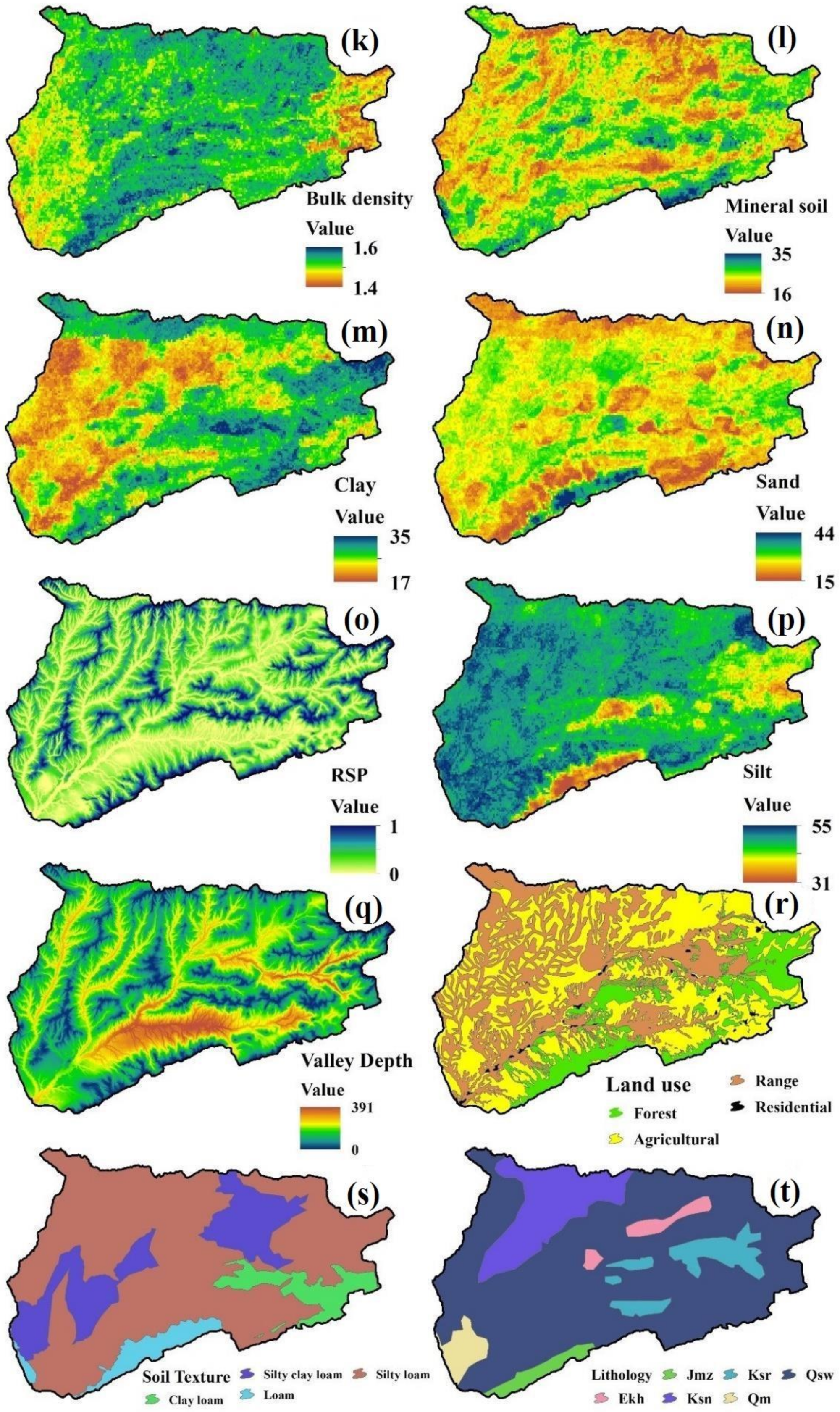
| Land Use | Area (he) | Area (%) |
|---|---|---|
| Forest | 12,513.04 | 15.95 |
| Residential Areas | 498.6 | 0.64 |
| Rangelands | 29,858.8 | 38.07 |
| Agricultural | 35,568.2 | 45.35 |
| Geo Unit | Description | Age | Area (ha) | Area (%) |
|---|---|---|---|---|
| Qm | Swamp | Cenozoic | 2169.48 | 2.77 |
| Qsw | Grey to block shale and thin layers of siltstone and sandstone | Cenozoic | 58,000.92 | 73.94 |
| Ksn | Ammonite bearing shale with interaction of limestone | Mesozoic | 9786.63 | 12.48 |
| Ksr | Grey thick—bedded limestone and dolomite | Mesozoic | 4906.5 | 6.26 |
| Jmz | Olive—green shale and sandstone | Mesozoic | 1857.68 | 2.37 |
| Ekh | Swamp | Cenozoic | 1715.73 | 2.19 |
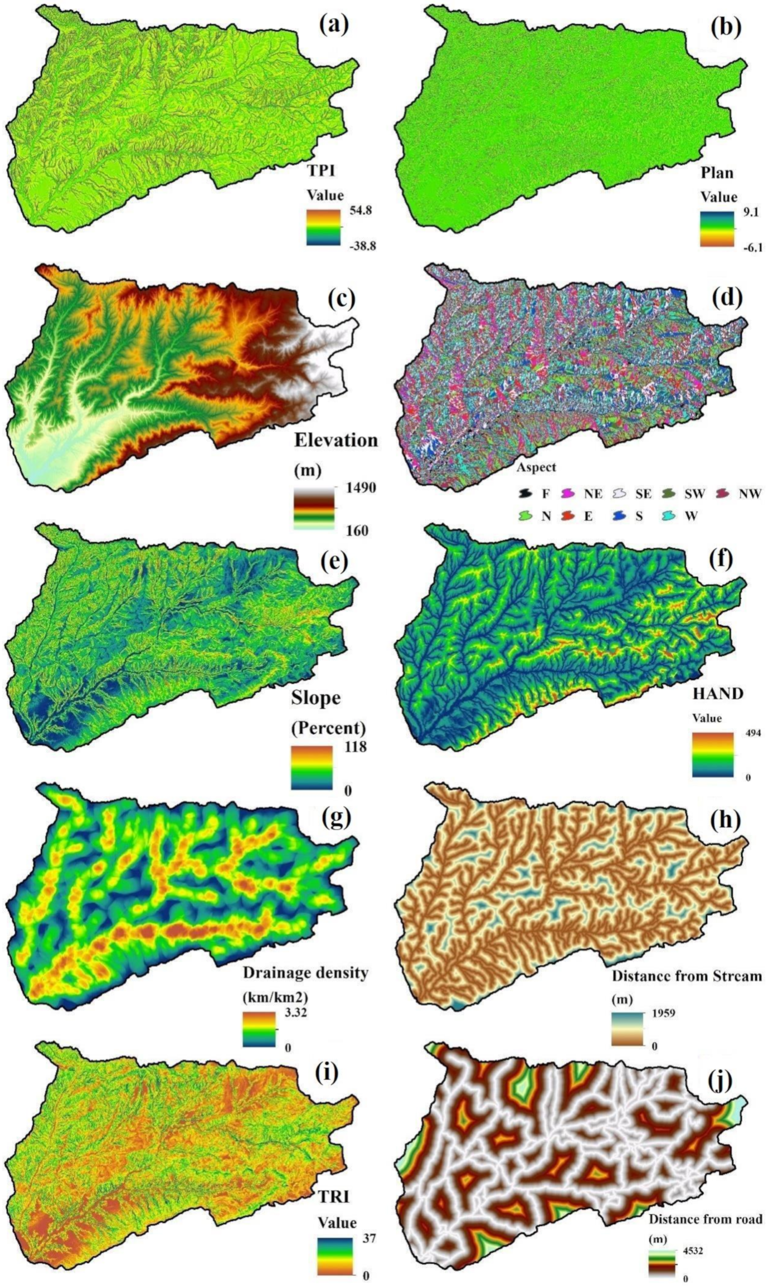
| Sl. No. | Conditioning Factors | Source | Time | Spatial Resolution/Scale |
|---|---|---|---|---|
| 1 | Topography position index (TPI) | ALOSPALSER DEM | 12/08/2012 | 12.5 mt. |
| 2 | Plan curvature | ALOSPALSER DEM | 12/08/2012 | 12.5 mt. |
| 3 | Elevation | ALOSPALSER DEM | 12/08/2012 | 12.5 mt. |
| 4 | Aspect | ALOSPALSER DEM | 12/08/2012 | 12.5 mt. |
| 5 | Slope | ALOSPALSER DEM | 12/08/2012 | 12.5 mt. |
| 6 | Height above nearest drainage (HAND) | ALOSPALSER DEM | 12/08/2012 | 12.5 mt. |
| 7 | Drainage density | ALOSPALSER DEM | 12/08/2012 | 12.5 mt. |
| 8 | Distance from stream | ALOSPALSER DEM | 12/08/2012 | 12.5 mt. |
| 9 | Train ruggness index (TRI) | ALOSPALSER DEM | 12/08/2012 | 12.5 mt. |
| 10 | Distance from road | Google Earth images, Landsat 8 satellite images by USGS and Topographical map by National Geographic Organization of Iran (www.ngo-org.ir) | 17/06/2019 | 30 mt. |
| 11 | Bulk density | Soil and Water Research Institute (SWRI) (http://www.iran.swri.com) | 18/06/2019 | 1:1,000,000 |
| 12 | Mineral Soil | Soil and Water Research Institute (SWRI) (http://www.iran.swri.com) | 18/06/2019 | 1:1,000,000 |
| 13 | Clay content | Soil and Water Research Institute (SWRI) (http://www.iran.swri.com) | 18/06/2019 | 1:1,000,000 |
| 14 | Sand content | Soil and Water Research Institute (SWRI) (http://www.iran.swri.com) | 18/06/2019 | 1:1,000,000 |
| 15 | Relative slope position (RSP) | ALOSPALSER DEM | 12/08/2012 | 12.5 mt. |
| 16 | Silt content | Soil and Water Research Institute (SWRI) (http://www.iran.swri.com) | 18/06/2019 | 1:1,000,000 |
| 17 | Valley depth | ALOSPALSER DEM | 12/08/2012 | 12.5 mt. |
| 18 | Land use | Google Earth images, Landsat 8 satellite images by USGS and Topographical map by National Geographic Organization of Iran (www.ngo-org.ir) | 17/06/2019 | 30 mt. |
| 19 | Soil Texture | Soil and Water Research Institute (SWRI) (http://www.iran.swri.com) | 18/06/2019 | 1:1,000,000 |
| 20 | Lithology | Geological Society of Iran (GSI) (http://www.gsi.ir/) | 14/07/2019 | 1:100,000 |
| Conditioning Factors | Collinearity Statistics | |
|---|---|---|
| Tolerance | VIF | |
| TPI | 0.923 | 1.079 |
| HAND | 0.921 | 1.118 |
| Valley depth | 0.916 | 1.124 |
| Lithology | 0.915 | 1.127 |
| Land use | 0.888 | 1.279 |
| RSP | 0.823 | 1.483 |
| Bulk density | 0.813 | 1.492 |
| Distance from road | 0.778 | 1.532 |
| Soil texture | 0.754 | 1.611 |
| Plan | 0.745 | 1.721 |
| Distance from stream | 0.743 | 1.865 |
| Mineral Soil | 0.739 | 1.897 |
| Slope | 0.728 | 1.932 |
| Drainage density | 0.425 | 2.364 |
| TRI | 0.387 | 2.624 |
| Elevation | 0.346 | 2.715 |
| Aspect | 0.345 | 2.817 |
| Silt | 0.233 | 3.534 |
| Clay | 0.313 | 3.696 |
| Sand | 0.231 | 4.749 |
| Row | Models | AUC | Prioritizing | ||
|---|---|---|---|---|---|
| Training | Validation | Priority Based on Training | Priority Based on Validation | ||
| 1 | GLM 90/10 | 0.826 | 0.818 | 14 | 10 |
| 2 | GLM 80/20 | 0.834 | 0.788 | 12 | 16 |
| 3 | GLM 70/30 | 0.837 | 0.79 | 11 | 15 |
| 4 | GLM 60/40 | 0.813 | 0.837 | 16 | 4 |
| 5 | GLM 50/50 | 0.833 | 0.816 | 13 | 11 |
| 6 | MaxEnt 90/10 | 0.809 | 0.784 | 18 | 17 |
| 7 | MaxEnt 80/20 | 0.821 | 0.764 | 15 | 18 |
| 8 | MaxEnt 70/30 | 0.81 | 0.799 | 17 | 13 |
| 9 | MaxEnt 60/40 | 0.786 | 0.819 | 20 | 9 |
| 10 | MaxEnt 50/50 | 0.808 | 0.796 | 19 | 14 |
| 11 | ANN 90/10 | 0.885 | 0.867 | 4 | 2 |
| 12 | ANN 80/20 | 0.91 | 0.804 | 3 | 12 |
| 13 | ANN 70/30 | 0.872 | 0.837 | 7 | 4 |
| 14 | ANN 60/40 | 0.917 | 0.825 | 2 | 8 |
| 15 | ANN 50/50 | 0.918 | 0.868 | 1 | 1 |
| 16 | SVM 90/10 | 0.87 | 0.864 | 8 | 3 |
| 17 | SVM 80/20 | 0.877 | 0.819 | 5 | 9 |
| 18 | SVM 70/30 | 0.875 | 0.828 | 6 | 7 |
| 19 | SVM 60/40 | 0.859 | 0.835 | 10 | 5 |
| 20 | SVM 50/50 | 0.866 | 0.834 | 9 | 6 |
© 2020 by the authors. Licensee MDPI, Basel, Switzerland. This article is an open access article distributed under the terms and conditions of the Creative Commons Attribution (CC BY) license (http://creativecommons.org/licenses/by/4.0/).
Share and Cite
Arabameri, A.; Asadi Nalivan, O.; Chandra Pal, S.; Chakrabortty, R.; Saha, A.; Lee, S.; Pradhan, B.; Tien Bui, D. Novel Machine Learning Approaches for Modelling the Gully Erosion Susceptibility. Remote Sens. 2020, 12, 2833. https://0-doi-org.brum.beds.ac.uk/10.3390/rs12172833
Arabameri A, Asadi Nalivan O, Chandra Pal S, Chakrabortty R, Saha A, Lee S, Pradhan B, Tien Bui D. Novel Machine Learning Approaches for Modelling the Gully Erosion Susceptibility. Remote Sensing. 2020; 12(17):2833. https://0-doi-org.brum.beds.ac.uk/10.3390/rs12172833
Chicago/Turabian StyleArabameri, Alireza, Omid Asadi Nalivan, Subodh Chandra Pal, Rabin Chakrabortty, Asish Saha, Saro Lee, Biswajeet Pradhan, and Dieu Tien Bui. 2020. "Novel Machine Learning Approaches for Modelling the Gully Erosion Susceptibility" Remote Sensing 12, no. 17: 2833. https://0-doi-org.brum.beds.ac.uk/10.3390/rs12172833