Agronomic Traits Analysis of Ten Winter Wheat Cultivars Clustered by UAV-Derived Vegetation Indices


Department of Agricultural, Environmental and Food Sciences (DAEFS), University of Molise, I-86100 Campobasso, Italy
*
Author to whom correspondence should be addressed.
Remote Sens. 2020, 12(2), 249; https://0-doi-org.brum.beds.ac.uk/10.3390/rs12020249
Submission received: 11 November 2019
/
Revised: 9 December 2019
/
Accepted: 8 January 2020
/
Published: 10 January 2020
(This article belongs to the Special Issue Remote Sensing for Crop Mapping)
Abstract
:Timely and accurate estimation of crop yield variability before harvest is crucial in precision farming. This study is aimed to evaluate the ability of cluster analysis based on Vegetation Indices (VIs) that were obtained from UAVs to predict the spatial variability on agronomic traits of ten winter wheat cultivars. Five VIs groups were identified and the ground truth yield-related data were analyzed for clusters validation. The yield data revealed a value of 6.91 t ha−1 for the first cluster with the highest VIs value and a decrease of −12%, −21%, and −27% for the 2nd, 3rd, and 4th clusters; respectively; the 5th cluster; with the lowest VIs value showed the lower yield values (4 t ha−1). Agronomic traits, such as dry biomass, spike numbers, and weight were grouped according to VIs clusters and analyzed and showed the same trends. The analysis of spatial distribution and agronomic data of the ten cultivars within the single clusters highlighted that the most productive varieties showing a greater value of spike weight and numbers and a greater presence of areas with high values of VIs and vice versa the less productive once, though two cultivars showed productions not linked to cluster classification and high data range variability were recorded. Cluster identified by high-resolution UAV vegetation indices can be a valid strategy although its effectiveness is closely linked to the cultivar component and, therefore, requires extensive verification.
1. Introduction
Wheat is the crop grown with the highest acreage (FAO stat, 2019), therefore monitoring the wheat crop growth and canopy biophysical parameters, yield and yield components within a season is essential to decision-makers [1]. Multiple interactions and mechanisms of compensation among the different yield components are related to genotype, environment, and agronomy interactions [2]. In a specific environmental condition and for a selected genotype, grain yield per area is affected by spikes per area, grain weight, and grains per spike [3].
In recent years, with the advancement of UAV technology, high-resolution georeferenced data can be obtained at relatively low cost. This has increased the interest in obtaining temporal and spatial canopy information and utilize it to improve management decisions and yield [4]. The main aim of precision agriculture in cropping systems is to deliver information that will allow for better management decisions [5] for improving crop quality and crop yield production and at the same time reducing environmental pollution and farming costs [6].
Remote sensing at visible and near-infrared wavelengths (vis-NIR) has been used to formulate many spectral indices for estimating crop properties [6,7]. Simple Vegetation Indices have significantly improved the ability and sensibility of the detection of green vegetation [8]. Vegetation indices are widely used to estimate crop growth status and crop parameters, such as biomass, yield, photosynthesis, Leaf Area Index, etc. [1,9,10,11,12,13], and many studies have analyzed the potential of using spectral reflectance indices in wheat starting from the early years of the century (e.g., Aparicio et al. [14]) and up to the present day (e.g., Schirrmann et al. [4]). High-resolution Vegetation Indices (VIs) may detect changes of wheat crop status and it might help to improve crop monitoring, nitrogen management, and crop yield estimation [15]. Furthermore, it is indeed known that yield prediction while using VIs in wheat can be accurate two months prior to harvest, because yield estimates stabilize [1] and especially during the flowering period, significant correlations between UAV-VIs and yield components were found [16,17].
For this reason, multispectral imagery with high-resolution, acquired by lightweight UAVs and multispectral sensors, have added a new dimension in precision agriculture, offering a standing potential for quantifying aerial observations of wheat crop under a variety of field-inputs [18]. Low altitude remote sensing equipped with Vis-NIR camera provides a new applied technology to monitor and detect the canopy crop status at small and large scales, very interesting and important thing, above all in agronomic experiments, where resource, space, and time constraints limit manual sampling [19].
However, the use of UAVs for agricultural monitoring is limited by the rendering into useful data in the identification of homogeneous areas with identified requirements for different treatments and management of the agronomic factors. Among methods utilized for detecting homogeneous area, clustering methods, such as k-means clustering, fuzzy k-means, partition around mediods, among vegetation indices, and crop and soil parameters for delineating management zones maps in a cultivar were used [4,6,16]. The clustering algorithm is used to partition all members of a population into one of several groups or clusters, such that the sum of squares for members within a cluster is minimized, while the sum of squares between the members of different clusters is maximized [20]. Even if we know that, as reported by Xue and Su [8], each VI has its specific expression of green vegetation and for real-world applications, the use of vegetation indices requires careful consideration of the strengths and shortcomings of those indices, the specific environment where they will be applied, and the different reflectance of each cultivar.
Cluster analysis can play an important role in differentiating field variability and locating the low and high producing regions. This will help farmers to make management decisions early in the season. Additionally, this research is based on the UAV data that were collected at anthesis and the researchers can highlight some more information on how this study can be useful in assessing field variability and predict grain yield at least a month before harvesting.
For these reasons, and since the UAV processing programs easily provide maps with different vegetation indices, we examined the ability of three different near-infrared vegetation indices, which are reported to be well correlated with biomass, to detect homogeneous area. VIs data recorded at anthesis stage by high-resolution UAV were clustered by Ward’s minimum variance approach. Geo-referred agronomic traits data that were collected at harvest were analyzed according to the identified VIs clusters data from an agronomic point of view.
The aim of the study was to analyze if the clusters based on vegetation indices data (NDVI, SAVI, and OSAVI) were linked to agronomic traits of ten winter wheat cultivars and the ability of clustered VIs to detect wheat spatial variability.
2. Materials and Methods
2.1. Study Area and Field Measurements
The on-farm research was carried out in Central Italy (Mosciano S. Angelo, Teramo) for the ten winter wheat cultivars in a flat area, at 65 m above sea level, in the 2015 crop season. The field of 1.8 hectares (411081.30E, 4730617.48N; UTM-WGS84 zone 33N) was cultivated with 10 plots of 1000 m2 each of winter wheat cultivars (Table 1).
Sowing of the wheat cultivars (Rebelde, Ambrogio, Artico C, Artico S, Arkeos, Akim, Artdecò, Arabia, Asuncion, and Catullo) was performed in December and the crop was harvested in July 2015. The amount of seeds per hectares was 200 kg for each cultivar and the previous crop was the soybean. Minimum-tillage was used. The fertilization was achieved with 200 kg ha−1 of P2O5 (27%) as basic fertilization and nitrogen fertilizer (35% N; 23% SO3—slow-release fertilizer) was applied at tillering and Booting/Stem elongation stage, respectively.
Meteorological data were collected by a weather station located in the experimental fields recorded total precipitation of 680 mm throughout the whole cropping season with a typical distribution of Mediterranean environments, greater in the winter months. The temperatures showed a typical trend of the area with December the coldest month (minimum value −1 °C) and July the hottest (maximum value 36.2 °C). Data were not recorded outside the norm of the period
Georeferenced plants sampling from 1 m2 were hand cut (nine samplings for each cultivar). The sampling area was randomly identified based on the crop spatial variability detected by low-resolution real-time orthoimages map. At the crop harvest stage [21], yield data, biomass, number, and weight of spike per square meter of each cultivar were measured. Dry mass, after oven drying fresh plant material (75 °C until constant weight), was determined.
2.2. UAV System and Flight Missions
The flights were carried out by a fixed-wing UAV eBee (senseFly, Cheseaux-sur-Lausanne, Switzerland), simultaneously with the plant samples. The flights were carried out from 12:30 p.m. to 1:30 p.m., at a flight altitude of 95 m above sea level, in stable ambient light conditions, with outstanding visibility and weak wind (below 5 m s−1). The imaged area of the experimental field of 12 hectares was recorded. At each sampling data, a first flight by visible spectrum (Canon Powershot S110) for visible RGB orthophoto was carried out. A second fly with a near infra-red photo camera for VIs calculation (Canon Powershot S110 NIR—maximum absorption of the green peak at 550 nm, of the red peak at 625 nm and NIR peak at 850 nm wavelengths), was performed. According to Gómez-Candón et al. [22], 80% of frontal and side overlap were used to avoid geometric distortion related to the flight at low altitude. Ten fixed targets (25 cm × 25 cm square) were placed across the field at the start date of the experiments as ground control points for orienting and relating the UAV images to the ground (uniform horizontal and vertical accuracy) and calibrate camera atmospheric and Albedo corrections) finally to overlay the multiple dates and map. The ground coordinates were recorded by Leica Viva—GS15 (Leica Geosystems AG, Cornegliano Laudense, Switzerland) with an accuracy of 0.025 m (horizontal) and 0.035 m (vertical).
2.3. Data Processing
The data processing was performed, as reported by Marino and Alvino [16]; acquired images were elaborated by Pix4D Ag to generate an accurately geo-referenced ortho-mosaicked image. The multiple images were merged and then ortho-rectified. Pix4D software, incorporates SIFT (scale-invariant feature transform) algorithm to match the key points across multiple images [23,24] and processes data in three steps: (1) an initial processing of camera internals and externals data, automated aerial triangulation, bundle block adjustment; (2) point cloud densification; and, (3) digital surface map and orthomosaic generation. The orthomosaic was georeferenced to UTM-WGS84 zone 33N Italy, the final outputs were an RGB GeoTIFF with a resolution of 5 cm pixel−1.
The Pix4D software generates the VIs map in the raster calculator. The resolution of the reflectance map has been set at 5 cm pixel−1. A GeoTIFF image with a resolution of 5 cm pixel−1 was generated for each VI.
2.4. Vegetation Indices
The Normalized Difference Vegetation Index (NDVI), the Soil Adjusted Vegetation Index (SAVI), and the Optimized Soil Adjusted Vegetation Index (OSAVI) were used to characterize crop cultivars at different growth stages at the field (Table 2).
The NDVI index was calculated based on the difference of the near infra-red (NIR) and the Red (RED) reflectance spectral bands, being normalized by the sum of the reflectance at these spectral bands. The NDVI ranges from 1.0 to −1.0, positive values are related to increasing greenness and negative values are related to non-vegetated features. NDVI has some weaknesses linked to the possibility of reaching saturation, in particular in later growth stages [28,29].
The SAVI was elaborated to account for the optical soil properties in the plant canopy reflectance. The constant L was introduced in order to minimize soil brightness. L factor ranging from 0 to infinity, depends on the canopy density. For the SAVI computation, the characteristics of the surveyed wheat area suggested an L value at the anthesis stage of 0.20 [30].
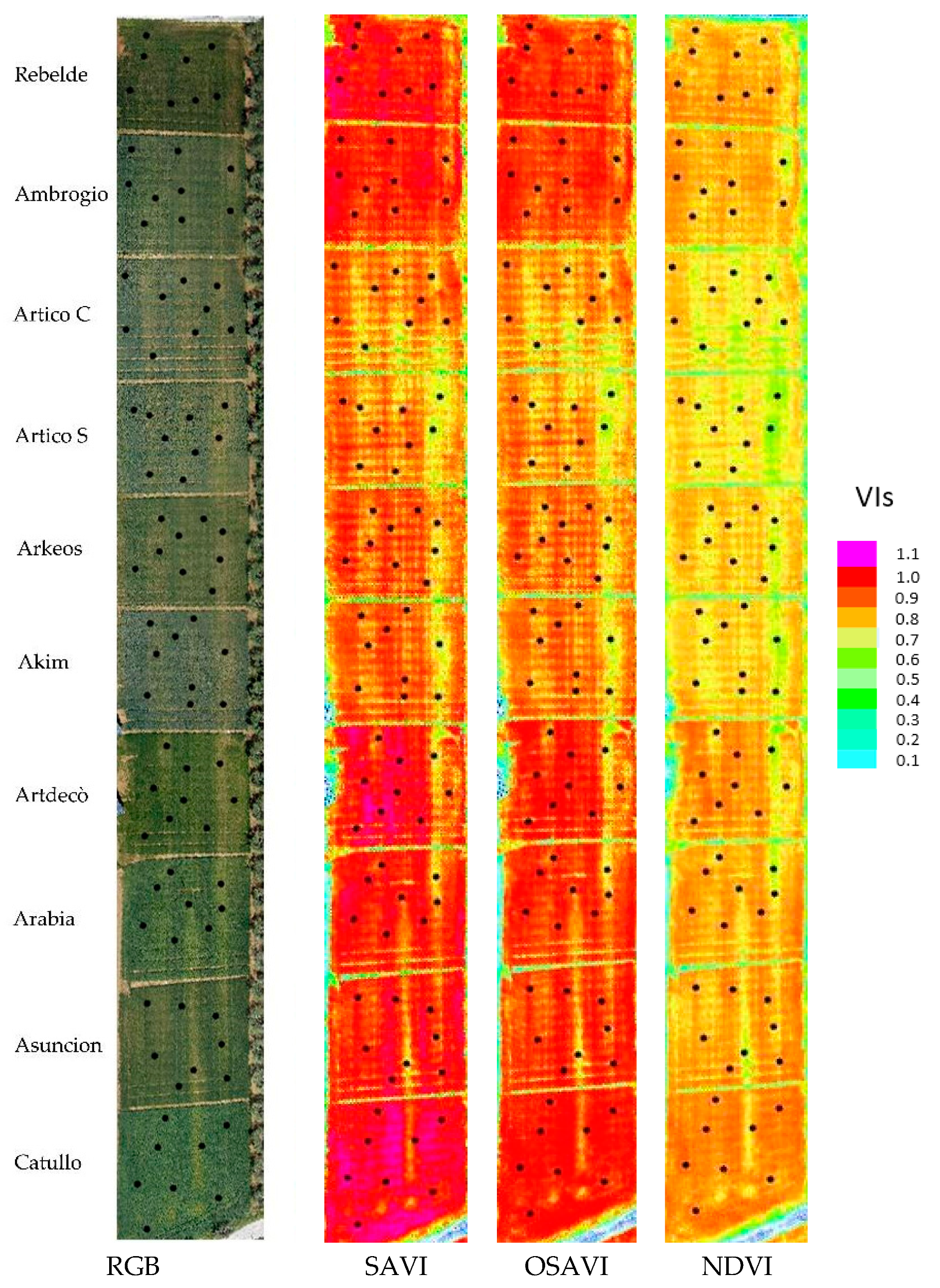
The OSAVI index was proposed by using bidirectional reflectance in the near-infrared and red bands. OSAVI is independent of soil-line and influence of the soil background effectivity. The soil adjustment coefficient (0.16) was selected as the optimal value to minimize the variation with the soil background. Figure 1 reports the SAVI, OSAVI, and NDVI maps.
2.5. Statistical Analysis
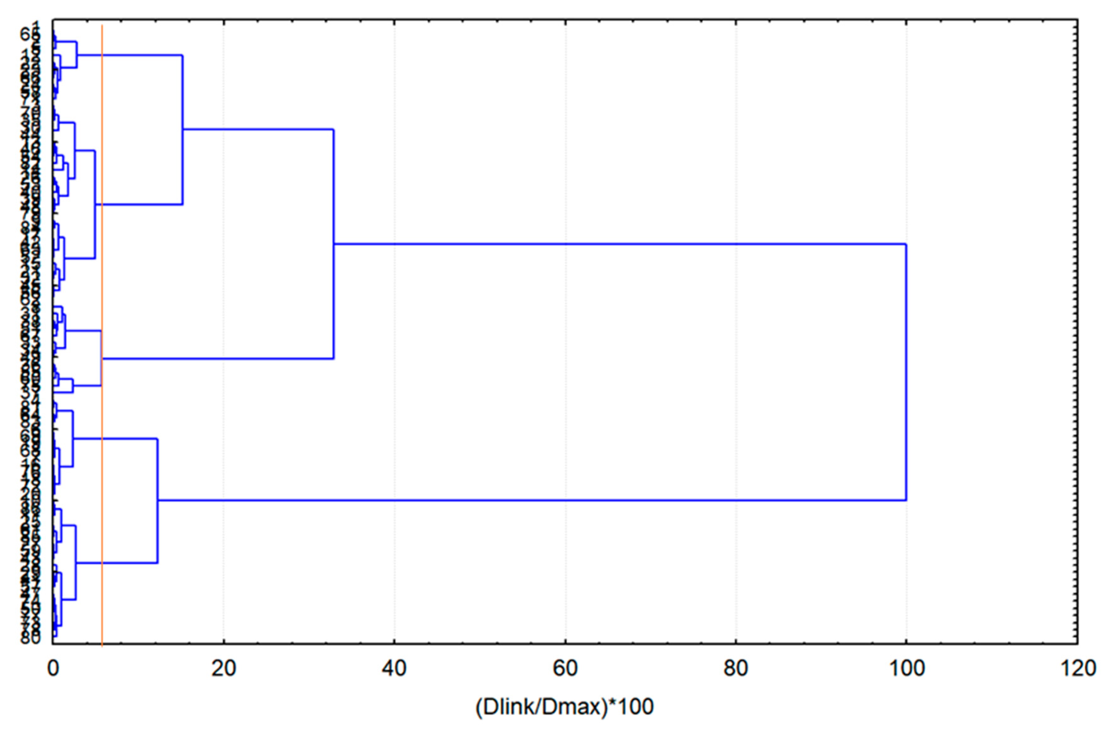
The VIs data were statistically processed while using the hierarchical clustering Ward’s minimum variance approach [31], as described in a previous paper that was published by Marino et al. [32]. The cluster analysis classifies observations into groups, in which the cluster members have common properties.
Based on the distance matrix, agglomerative clustering first selects the most similar two groups and afterwards merges them into a single group. The procedure is repeated until all of the samples have been added to a single large cluster and the final partition is identified by a distance criterion [33]. Starting from the bottom part of the dendrogram (Appendix A), the researcher decides to stop the agglomeration process when successive clusters are too far apart to be merged. In the present paper, the groups were merged and created on the three identified VIs (NDVI, SAVI, and OSAVI). The statistical VIs median values, standard deviations, and analysis of variance between the clusters and within the clusters are reported in Table 3. Statistical tests were used to verify the dependence conditioning of the different variables (a posteriori). The scree plot to choose the significant number of clusters was used [34]. The multivariate statistical technique of principal component analysis (PCA) was applied to the whole set of studied agronomic traits that were grouped according to identified VIs clusters, to transform the data into a set of uncorrelated orthogonal variables. OriginPRO 8 (Origin Lab Corporation, Northampton, MA 01060, USA) and STATISTICA (Stat Soft., Inc., Oklahoma, OK, USA) were used for statistical analysis.
3. Results
3.1. Cluster Analysis Based on VIs Data
High-resolution Vegetation Indices data of ten winter wheat cultivars that were collected at anthesis were clustered to detect group data with significant differences. Starting from 86 georeferenced points of each VI (NDVI, SAVI, and OSAVI) at anthesis, hierarchical clustering Ward’s minimum variance approach was used for identifying the clusters. Five clusters were identified (Table 3), the cluster differences among VIs increased, starting from the 5th cluster (lowest values) to the 1st cluster (highest).
The median value of SAVI within each cluster was 1.03 for the 1st group, 0.96 for the 2nd group, 0.86 for the 3rd group, 0.79 for the 4th group, and 0.67 for the 5th group. Among the neighbour groups of each VI, differences that ranged from 6 to 10% were recorded, except for the 5th group that showed median value differences of −17% for both SAVI and OSAVI, and −12% for NDVI with respect to the 4th group. The VIs median value of the 5th cluster was 37% (SAVI and OSAVI) and 31% (NDVI) lower than the 1st cluster.
3.2. Agronomic Data Based on VIs Clusters
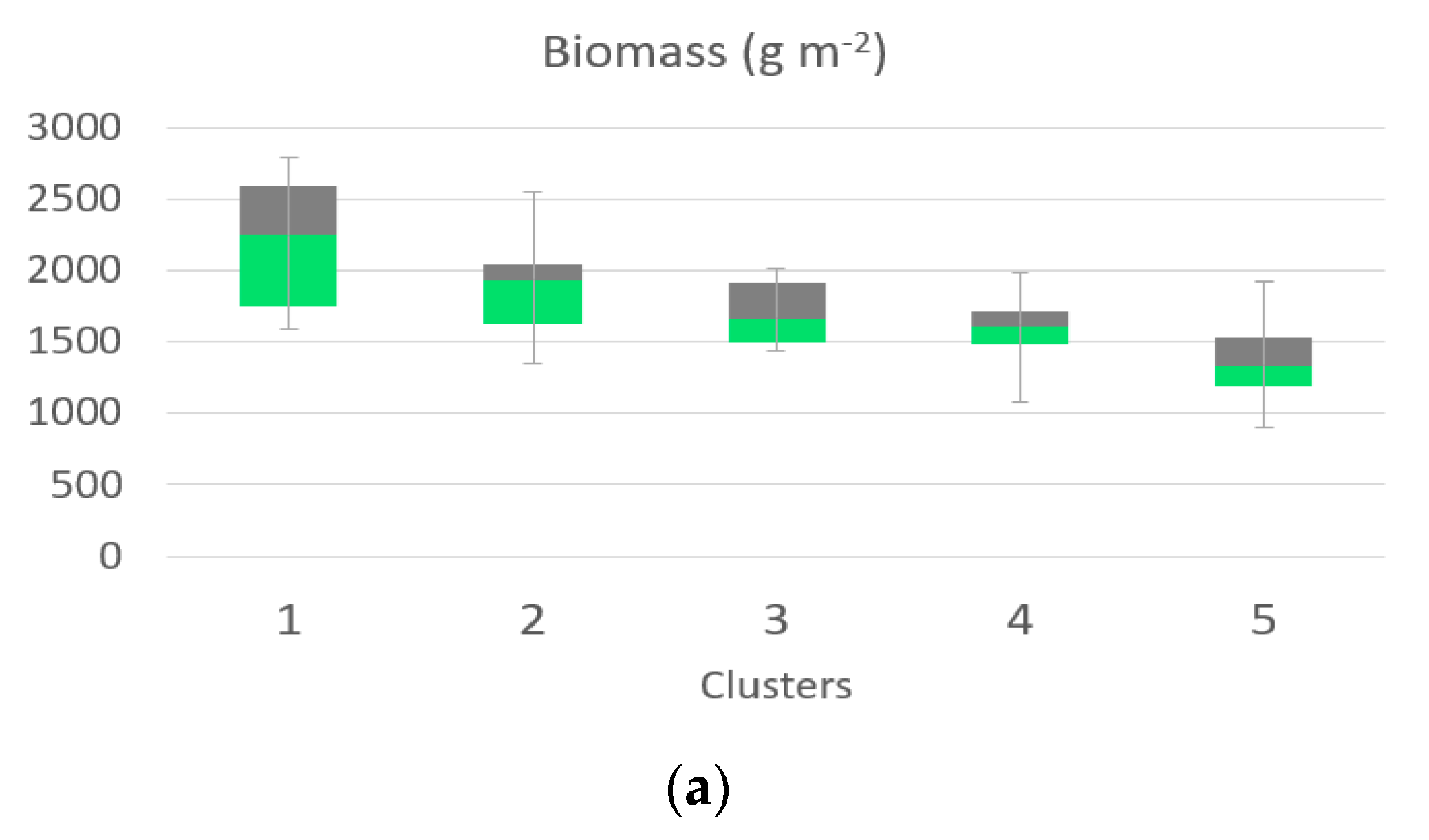
The agronomic traits of the ten wheat cultivars that were collected at harvest were analyzed according to the VIs clusters’ separation presented in Table 3. Figure 2 shows the box plots of the five clusters of the most important parameters for winter wheat: (a) for the total yield, (b) the dry biomass, (c) the spike number, and (d) for the spike weight. The box plot is a statistic method of displaying the data distribution based on the median value, minimum, first quartile, median, third quartile, and maximum.
The dry biomass data, which range from 2244 (g m−2) for the 1st cluster and decreasing by 1935 (g m−2) for the 2nd cluster, 1666 (g m−2) for the 3rd cluster, 1615 (g m−2) for the 4th cluster, and a dry mass of 1329 g m−2 for the 5th cluster (−41% respect to the 1st cluster). A larger variability characterized the distribution of cluster 1. A similar trend was recorded for the yield data, that ranged from 6.91 t ha−1 for the 1st cluster (highest VIs value), to 4 t ha−1 for the 5th cluster (with the lowest VIs value). The yield median value recorded for the 2nd cluster was 6.1 t ha−1, followed by the 3rd cluster 5.5 t ha−1 and 50.5 for the 4th cluster.
The spike weight of clusters 1 was 843 (g m−2), followed by cluster 2 with a value of 742 (g m−2), the third and fourth clusters showed values of 660 (g m−2) and 634 (g m−2) respectively. The spike numbers of the 1st cluster showed a median value of 532 spikes per square meters, the other clusters showed a lower number of spikes per square meters with 466, 444, 381, and 328 for cluster 2, cluster 3, cluster 4, and cluster 5, respectively.
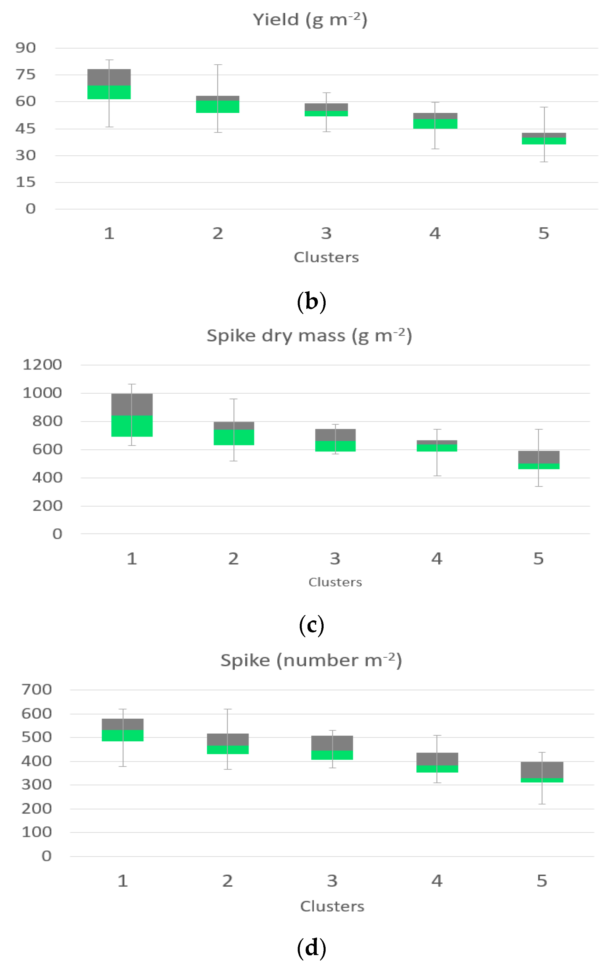
A principal component analysis (PCA) transformation was applied to the agronomic traits according to VIs data to understand whether differences between clusters are meaningful or not.
A close inspection of the PCA combining the agronomical traits of the different identified cluster demonstrates that VIs grouped similar crop attributes and how they are related to the different identified cluster. There was a little difference noted between the 1st and 2nd cluster and between the 3rd and 4th identified cluster (Figure 3).
The PCA showed that the first two components explained 72% of the variation (Figure 3). The Agronomic traits that had a strong and positive contribution to the first component (PC1—47.70% of variance) were the agronomic traits of the 1st and 2nd cluster, whereas the agronomic traits of the 5th cluster were negatively correlated.
3.3. Cluster Map Based on VIs Data and Agronomic Variability Among and Within Cultivars
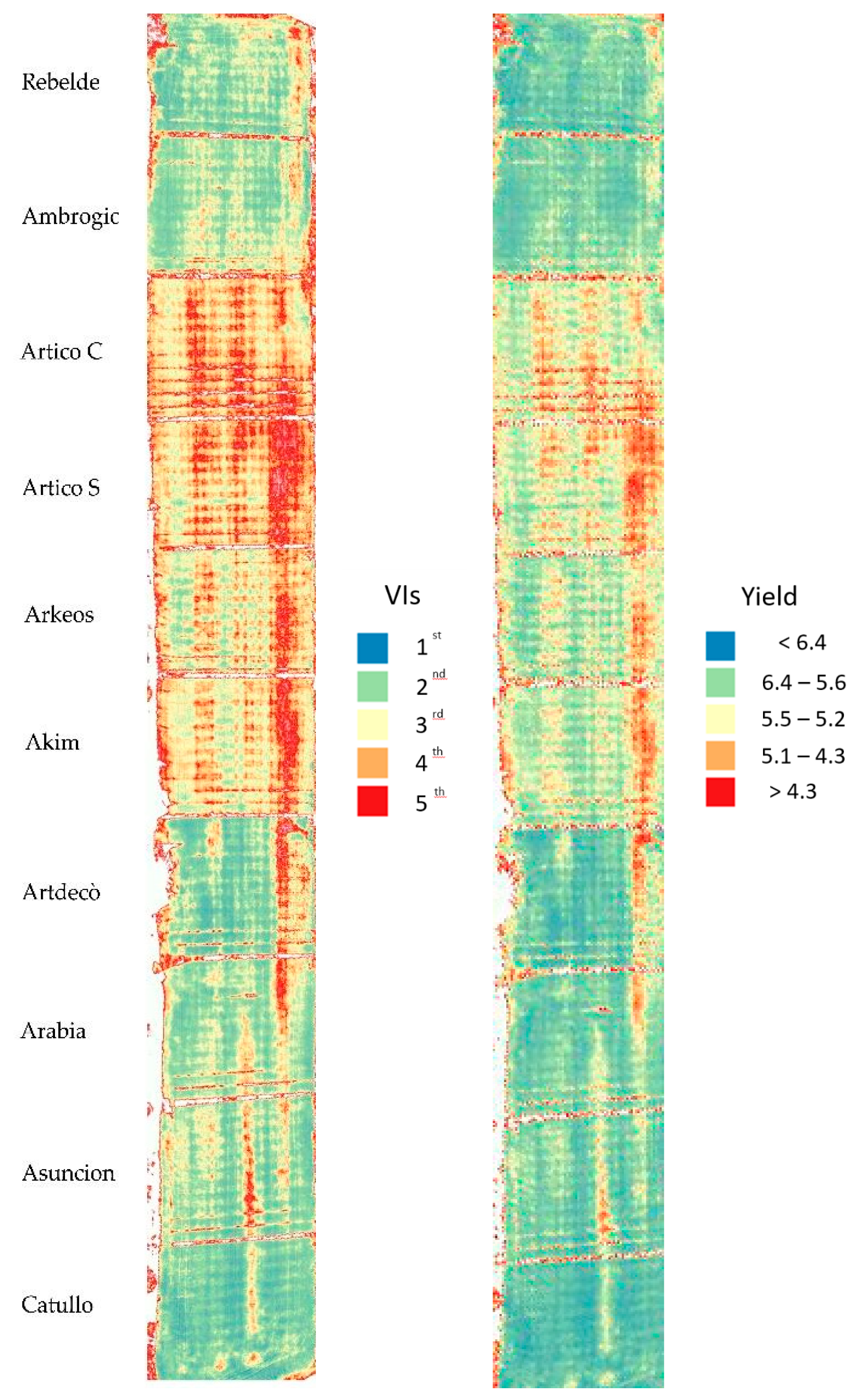
The clusters map was elaborated according to the clustered VIs and the analysis of agronomic traits of the sampling collected at harvest in the same georeferenced points were performed (Figure 4, sx). The map reports five different colors, starting from the red for the 1st cluster (highest VIs values) to the blue one (lowest VIs value). At a visual assessment, the map highlights clear differences among the ten cultivars and the spatial variability within each of them. The VIs data of the 1st cluster were only detected in six cultivars, which were distributed over wide surfaces in Rebelde, Ambrogio, Artdecò, and Catullo and over small surfaces in Arabia and Asuncion. While the VIs data of the other four clusters were present in all cultivars. The four cultivars with no VIs data in the 1st cluster (Artico S., Artico C, Arkeos and Akim) also showed small surfaces of the 2nd cluster. Furthermore, Artico S., Artico C showed a large area in the 5th cluster, followed by Arkeos and Akim, and finally by other cultivars with small surfaces. The cultivars with a wide area in the highest VIs clusters (1st and 2nd) were characterized by high crop yield and yield components. Five of the six cultivars with wide surfaces in the 1st VIs cluster (Catullo, Asuncion, Arabia, Artdecò, and Ambrogio) also showed the highest values for yield, biomass, spikes number, and weight. The cultivars Artico C, Artico S, and Arkeos that were characterized by wide surfaces of low VIs values (4th and 5th clusters) showed a medium agronomic response.
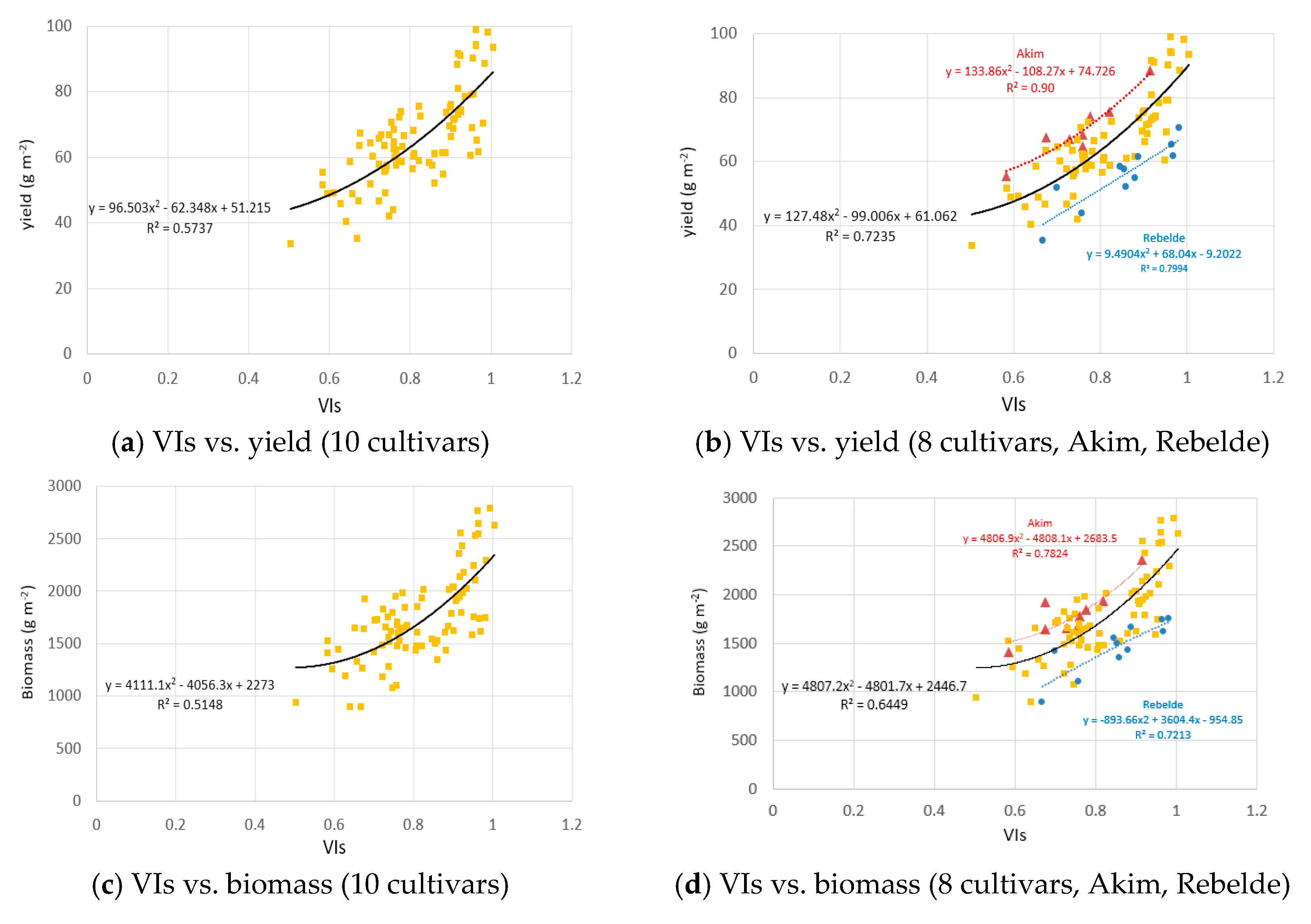
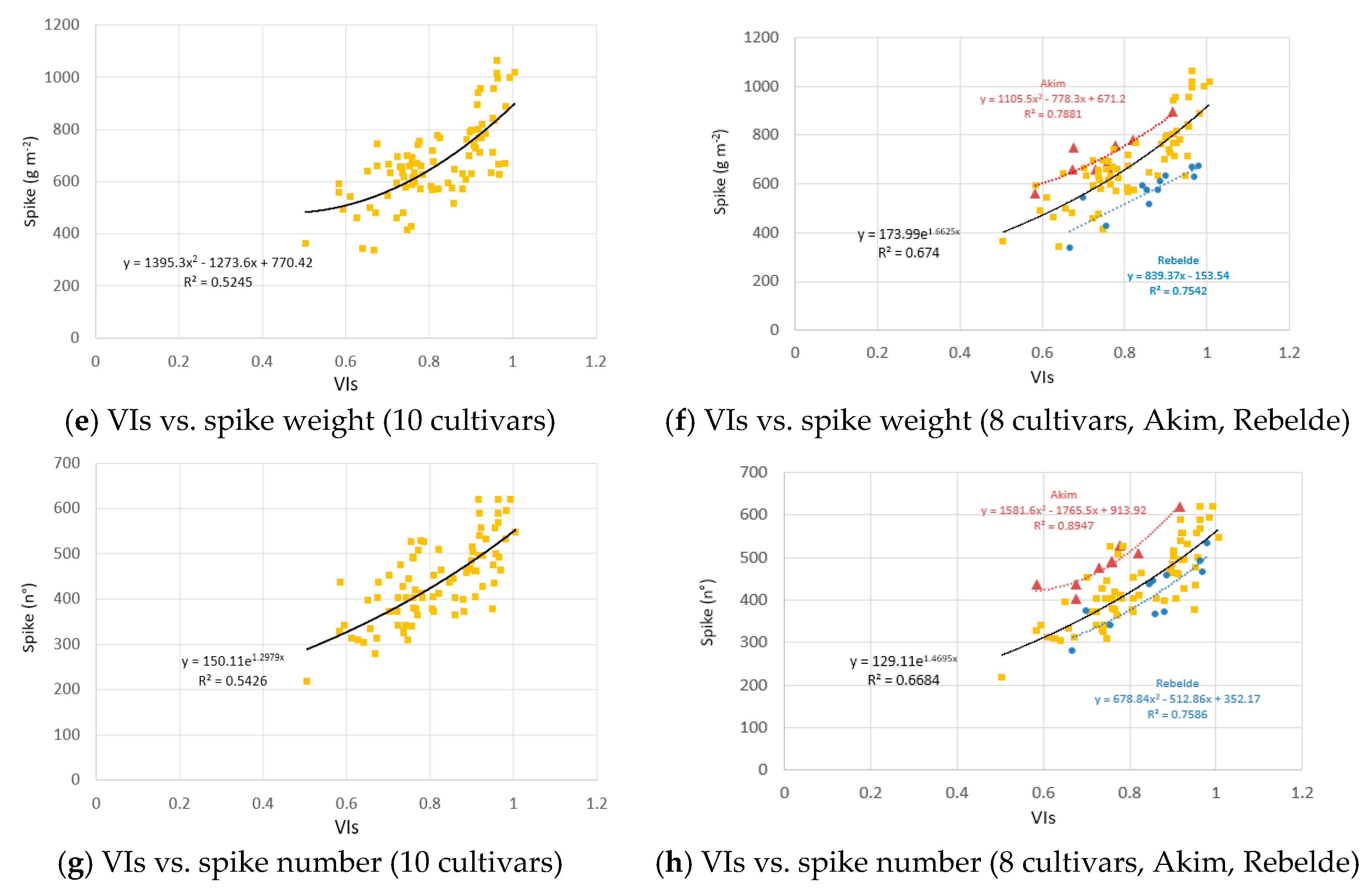
Within the ten cultivars, under the same VIs values, Rebelde showed the lowest yield and yield components data, while Akim showed the highest yield and agronomic traits values (Appendix B).
The two functions were parallel and they delimit at the bottom and top the relationship of the other eight cultivars. A polynomial function with an R2 of 0.72 was recorded between VIs vs yield ground truth data of the eight cultivars (excluding Akim and Rebelde cultivars), the regression value of the ten cultivars drops to R2 = 0.57. The same trend and similar function were recorded for the biomass data, with an R2 of 0.65 while excluding Akim and Rebelde and R2 = 0.51 if included. Spike weight showed a polynomial function with R2 = 0.67 and R2 = 0.52 without and with Akim and Rebelde, respectively. The spike number showed an exponential function and value of R2 = 0.54 and R2 = 0.67 without and with Akim and Rebelde, respectively
Based on the VIs-yield regression, a map was elaborated and reported in Figure 4 (dx) for evaluating the ability to assess the field variability between clusters formed based on VIs and ground samples. At visual assessment, the map showed few differences in the discrimination of the areas and confirms the analysis reported previously; a smoothing of the yield clusters data with respect to the UAV-derived VIs clusters is also evident.
4. Discussion
The Unmanned Aerial Vehicles (UAV) offer greater flexibility in flight scheduling, which makes it a useful tool for researchers and farmers to monitor and manage crops at the field scale [35]. The UAV allows for the acquisition of data and images with high spatial resolution (sub centimeter) [36], although the high number of data is restricted the fields of application due to the difficulty of easily identifying a management strategy linked to areas with the same variability. Most of the scientific papers identify areas with similar characteristics starting from the combination of agronomic traits and soil data on the ground with vegetation indices, which makes it difficult to apply these methods starting exclusively from UAV-derived VIs data. Moreover, among all of the elaborated VIS, some are certainly more efficient, among which SAVI, OSAVI and NDVI, have been widely used with good results [37,38]. This work explores the ability of cluster analysis, based on the combination of three of the most widely used vegetation indices, to identify the population groups with homogeneous VIs and, subsequently, evaluate whether the identified groups have a link with the main agronomic data (yield and yield components) related to spatial variability of 10 wheat varieties.
4.1. Cluster Analysis Based on VIs Data
Five clusters were identified by the cluster analysis on UAV-derived VIs data. The 1st cluster showed the higher values for all three indices investigated, from the second to the fourth cluster the distance between groups fell by an average value of −6% −10%, with the fifth group being far away with −12% −17% when compared to the fourth cluster. The VIs cluster median values showed the higher values for SAVI and OSAVI indices, NDVI highlighted the lowest maximum values and the narrowest data range, confirming the results that were achieved by Marino and Alvino (2018) in previous work on durum wheat. The NDVI median values recorded −15% and −12% differences than the SAVI and OSAVI ones. Moreover, the wider range of values of both SAVI and OSAVI indices favoring better data discrimination among clusters, in fact the difference between the medians of 1st and 5th clusters was 0.38 for SAVI and 0.27 for NDVI, showing that, in an open field experiment, the distance between groups is very close and SAVI index showed high discrimination.
4.2. Agronomic Data Based on VIs Clusters
Agronomic ground truth georeferenced data of biomass, yield, spike weight, and spike number of ten wheat cultivars that were collected at harvest were analyzed according to the five identified clusters.
The dry biomass, yield, spike weight, and spike number data showed the highest values for the 1st cluster and decreasing values for clusters that range from 2nd to 5th.
The dry biomass data, ranging from 2244 (g m−2) for the 1st cluster and decreasing by 14% for the 2nd cluster, 26% for the 3rd cluster, 28% for the 4th cluster, and a dry mass of 1329 g m−2 for the 5th cluster (−41% with respect to the 1st cluster). As far as the analysis of biomass data by the identified clusters is concerned, we can say that clusters 3 and 4 showed a very close data of the medians, whereas those of clusters 1, 2, and 5 are well spaced.
A significant difference in the yield values was recorded; yield median value has passed from 6.91 t ha−1 recorded for the 1st cluster, to 4 t ha−1 for the 5th cluster. Moreover, starting from the 1st cluster, a decrease of 12%, 21%, and 27% was recorded for the 2nd, 3rd, and 4th clusters, respectively. The 5th cluster showed a reduction of more than 40%, proving the ability of the UAV-derived VIs cluster to identify areas with homogeneous production classes already at the anthesis.
The breadth distribution of data in the clusters 1, 2, and 4 was higher than the others, due to a higher residual variation occurring within each cluster.
The cluster median value of spike weight of clusters 1 was higher than the other four clusters (2nd, 3rd, 4th, 5th) that recorded a media values −12%, −22%, −25%, and −41%, respectively, than the 1st cluster. The spike numbers of the 1st cluster showed a median value of 531 spikes per square meters, the other clusters showed a reduction of −12%, −16%, −28%, and −38% with the lowest median value for the 5th cluster of 330 spikes per square meters.
The distribution of spike weight of clusters 1 was characterized by a larger variability, which suggests that the filling of the ears plays a strategic role in yield and biomass production.
The difference of cop yield was also explained by the differences of spike numbers in fact, it has gone from 531 ears per square meter for the 1st cluster to only 330 for the areas of the 5th cluster, but also with significant reductions for the intermediate clusters that have seen a reduction that has affected yield production.
The high spatial variability within fields has been widely stated for agronomical parameters, especially for the growth of wheat plants because it is influenced by a complex interrelation of many factors, such as natural environmental factors (such as radiation, temperature, rainfall, soil texture, and topography), management technologies (such as water and nitrogen fertilizer management), in addition to genotype [39,40].
Although the differences among the clusters of all the components analyzed are significant, the overlapping of many quartiles of the different groups determines the need to be very careful in managing the agronomic field management starting by VIs clusters.
A principal component analysis (PCA) applied to the agronomic traits clustered according to VIs data were performed to understand whether the differences between clusters are meaningful or not. PCA confirms the ability of cluster method to group samplings with similar attributes, highlighting as the first and second cluster had a strong and positive contribution to the first component, followed by the second and third clusters; the 5th cluster were negatively correlated.
These results showed how clusters 1 and 2, as well as 3 and 4, have agronomic attributes that are very close to each other. In particular, clusters 3 and 4 showed very close values of biomass, yield, and weight of the ears, with cluster 4 showing values lower by 3 to 8% when compared to cluster 3. Clusters 1 and 2 showed more marked differences between them, with lower values for cluster 2 by 12 to 14%. On the other hand, cluster 5, always shows much lower values than other clusters, by a reduction of about 40% as compared to cluster 1 for all of the agronomic parameters analyzed. This information can be extremely interesting for the evaluation and the choice of the management of cultural practices in the open field.
4.3. Cluster Map Based on VIs Data and Agronomic Variability Among and Within Cultivars
The map elaborated according to the clustered VIs at anthesis and the map elaborated according to the clustered VIs and the analysis of yield data of the ground truth georeferenced sampling collected at harvest report the different identified groups. Clear was the differences among the ten cultivars and the spatial variability within each of them. It is important to underline that not all of the cultivars have shown the same trends and the same distribution between clusters, in fact there are there are as many as four cultivars that do not have data in the first cluster and a lower surface in the second one (Artico S., Artico C, Arkeos, and Akim) by registering a large area in the 5th cluster. These cultivars also showed the lowest values related to the agronomic parameters analyzed, except Akim, which showed high average in yield productions and a relationship VIs-agronomic trait different from the other varieties. The VIs data of the 1st cluster were only detected in six cultivars (in Rebelde, Ambrogio, Artdecò, and Catullo with high involved surface and Arabia and Asuncion followed by small surfaces. As reported, the relationship among the six cultivars and agronomic traits confirm that crop characterized by highest VIs clusters (1st and 2nd) recorded high crop yield and yield components value. Even if, among these varieties, a different trend has been recorded by Rebelde that in the face of a large area between cluster 1 and 2 has shown much lower values of yield and yield components. Rebelde and Akim showed a different VIs–agronomic traits relationship for the inter-cultivar identification, they are in fact present at the edges of the regressions identified, which shows how important it is to analyze the agronomic parameters to be able to carry out a prediction or a precision management at the farm level. The regression between the UAV-derived VIs and the yield confirms that the yield values have been smoothed, which highlights a slight difference between the maps, but also an excellent capacity of this method of making important information for crop management if cultivars with different trends are excluded.
The analysis of agronomic data that were related to different cultivars with the same crop and environmental conditions is complex. The cases under examination point out an interesting trend between agronomic characteristics and spectroradiometric response. Although some cultivars have shown a completely different trend, not in line with the spectroradiometric responses of most cultivars. Many authors, such as Hassan et al. [17] and Duan et al. [19], Marino et al., [41] report the rapid assessment of VIs from UAV dynamic monitoring and predicting of the biomass change and grain yield during the growing season of wheat. In the present study, a significant correlation between agronomic parameters were revealed for each cultivar and VIs, but showed some limitations and weaknesses in the inter-cultivar analysis, since each cultivar has a specific own spectral response and function yield-VIs as stated before. According to Hassler and Baysal-Gurel [42], the potential of UAS in agriculture is very high, and the eBee fixed-wing UAV has been demonstrated to be a good tool for agronomic purposes on wheat [43].
5. Conclusions
The study, based on one-year on-farm experiment on ten winter-wheat cultivars, the records results of a cluster analysis performed on different VIs at anthesis with the aim to study the agronomic variability of the whole field, among cultivars and within plots. Five VIs clusters were identified, starting from UAV maps of NDVI, OSAVI, and SAVI indices. Agronomic traits of all cultivars collected at anthesis and grouped according to VIs clusters showed significant yield and yield traits differences. The yield median value of each cluster of the population was 6.9, 6.1, 5.5, 5.1, and 4.0 t ha−1, respectively, even if a great variability was recorded. Little agronomic traits differences were noted between the 1st and 2nd cluster and between the 3rd and 4th identified cluster. Above all of the agronomic traits, spike weight showed a strong connection to the yield and biomass. The analysis of the map elaborated according to VIs clusters and analyzed in relationship with ground sampling data showed a significant ability of VIs clusters to detect the boundaries within the cultivars (discriminate against more and less productive areas) and a good tendency to define differences among cultivars. The regression among VIs and agronomic traits of each cultivar was different and only the exclusions of two varieties (Akim and Rebelde) results in good VIs-Yield regression.
Therefore, the identification (and management) of wheat spatial variability can be negatively affected if it is carried out with no ground-truth validation.
Author Contributions
Authors contributed equally to this work. All authors have read and agreed to the published version of the manuscript.
Funding
This research did not receive any specific grant from funding agencies in the public, commercial, or not-for-profit sectors.
Acknowledgments
The authors are grateful to Giancarmine Montalto (Molise Geodetica) in charge of UAV flights.
Conflicts of Interest
The authors declare no conflict of interest.
Appendix A
Figure A1.
Tree diagram (dendrogram) for 86 cases Ward’s methods Euclidean distances.

Appendix B
Figure A2.
VIs vs. yield (a), biomass (c), spike weight (e), spike number (g)regression (R2 and polynomial functions) of 10 cultivars (yellow) (Left) and VIs vs. yield (b), biomass (d), spike weight (f), spike number (h) regression (R2 and polynomial functions) of 8 cultivars (yellow); cultivar Akim (red) and cultivar Rebelde (blue).


References
- Magney, T.S.; Eitel, J.U.H.; Huggins, D.R.; Vierling, L.A. Proximal NDVI derived phenology improves in-season predictions of wheat quantity and quality. Agric. For. Meteorol. 2016, 217, 46–60. [Google Scholar] [CrossRef]
- Slafer, G.A.; Savin, R.; Sadras, V.O. Coarse and fine regulation of wheat yield components in response to genotype and environment. Field Crops Res. 2014, 157, 71–83. [Google Scholar] [CrossRef]
- Philipp, N.; Weichert, H.; Bohra, U.; Weschke, W.; Schulthess, A.W.; Weber, H. Grain number and grain yield distribution along the spike remain stable despite breeding for high yield in winter wheat. PLoS ONE 2018, 13, e0205452. [Google Scholar] [CrossRef] [PubMed] [Green Version]
- Schirrmann, M.; Giebel, A.; Gleiniger, F.; Pflanz, M.; Lentschke, J.; Dammer, K.H. Monitoring Agronomic Parameters of Winter Wheat Crops with Low-Cost UAV Imagery. Remote Sens. 2016, 8, 706. [Google Scholar] [CrossRef] [Green Version]
- Whelan, B.; Taylor, J. Precision Agriculture for Grain Production Systems; CSIRO Publishing: Collingwood, Australia, 2013; pp. 1–2. [Google Scholar] [CrossRef] [Green Version]
- Chlingaryan, A.; Sukkarieh, S.; Whelan, B. Machine learning approaches for crop yield prediction and nitrogen status estimation in precision agriculture: A review. Comput. Electron. Agric. 2018, 151, 61–69. [Google Scholar] [CrossRef]
- Alvino, A.; Marino, S. Remote Sensing for Irrigation of Horticultural Crops. Horticulturae 2017, 3, 40. [Google Scholar] [CrossRef] [Green Version]
- Xue, J.; Su, B. Significant remote sensing vegetation indices: A review of developments and applications. J. Sens. 2017, 2017. [Google Scholar] [CrossRef] [Green Version]
- Marti, J.; Bort, J.; Slafer, G.A.; Araus, J.L. Can wheat yield be assessed by early measurements of Normalized Difference Vegetation Index? Ann. Appl. Biol. 2007, 150, 253–257. [Google Scholar] [CrossRef]
- Marino, S.; Alvino, A. Hyperspectral vegetation indices for predicting onion (Allium cepa L.) yield spatial variability. Comput. Electron. Agric. 2015, 116. [Google Scholar] [CrossRef]
- Marino, S.; Alvino, A. Proximal sensing and vegetation indices for site-specific evaluation on an irrigated crop tomato. Eur. J. Remote Sens. 2014, 47, 271–283. [Google Scholar] [CrossRef]
- Marino, S.; Basso, B.; Leone, A.P.; Alvino, A. Agronomic traits and vegetation indices of two onion hybrids. Sci. Hortic. 2013, 155, 56–64. [Google Scholar] [CrossRef]
- Basso, B.; Cammarano, D.; Cafiero, G.; Marino, S.; Alvino, A. Cultivar discrimination at different site elevations with remotely sensed vegetation indices. Ital. J. Agron. 2011, 6, 1–5. [Google Scholar] [CrossRef]
- Aparicio, N.; Villegas, D.; Casadesus, J.; Araus, J.L.; Royo, C. Spectral vegetation indices as nondestructive tools for determining durum wheat yield. Agron. J. 2000, 92, 83–91. [Google Scholar] [CrossRef]
- Cabrera-Bosquet, L.; Molero, G.; Stellacci, A.; Bort, J.; Nogués, S.; Araus, J. NDVI as a potential tool for predicting biomass, plant nitrogen content and growth in wheat genotypes subjected to different water and nitrogen conditions. Cereal Res. Commun. 2011, 39, 147–159. [Google Scholar] [CrossRef]
- Marino, S.; Alvino, A. Detection of homogeneous wheat areas using multi-temporal UAS images and ground truth data analyzed by cluster analysis. Eur. J. Remote Sens. 2018, 51, 266–275. [Google Scholar] [CrossRef] [Green Version]
- Hassan, M.A.; Yang, M.; Rasheed, A.; Yang, G.; Reynolds, M.; Xia, X.; Xiao, Y.; Hea, Z. A rapid monitoring of NDVI across the wheat growth cycle for grain yield prediction using a multi-spectral UAV platform. Plant Sci. 2019, 282, 95–103. [Google Scholar] [CrossRef]
- Latif, M.A.; Cheema, M.J.M.; Saleem, M.F.; Maqsood, M. Mapping wheat response to variations in N, P, Zn, and irrigation using an unmanned aerial vehicle. Int. J. Remote Sens. 2018, 39, 7172–7188. [Google Scholar] [CrossRef]
- Duan, T.; Chapman, S.C.; Guo, Y.; Zheng, B. Dynamic monitoring of NDVI in wheat agronomy and breeding trials using an unmanned aerial vehicle. Field Crops Res. 2017, 210, 71–80. [Google Scholar] [CrossRef]
- Jaynes, D.B.; Kaspar, T.C.; Colvin, T.S.; James, D.E. Cluster Analysis of Spatiotemporal Corn Yield Patterns in an Iowa Field. Agron. J. 2003, 95, 574–586. [Google Scholar] [CrossRef]
- Zadoks, J.C.; Chang, T.T.; Konzak, C.F. A decimal code for the growth stages of cereals. Weed Res. 1974, 14, 415–421. [Google Scholar] [CrossRef]
- Gómez-Candón, D.; De Castro, A.I.; López-Granados, F. Assessing the accuracy of mosaics from unmanned aerial vehicle (UAV) imagery for precision agriculture purposes in wheat. Precis. Agric. 2014, 15, 44–56. [Google Scholar] [CrossRef] [Green Version]
- Küng, O.; Strecha, C.; Beyeler, A.; Zufferey, J.-C.; Floreano, D.; Fua, P.; Gervaix, F. The accuracy of automatic photogrammetric technique on ultra-light UAV imagery. ISPRS Int. Arch. Photogramm. Remote Sens. Spat. Inf. Sci. 2012, XXXVIII-1/C22, 125–130. [Google Scholar] [CrossRef] [Green Version]
- Pajares, G. Overview and current status of remote sensing applications based on unmanned aerial vehicles (UAVs). Photogramm. Eng. Remote Sens. 2015, 81, 281–330. [Google Scholar] [CrossRef] [Green Version]
- Rouse, J.W.; Haas, R.H.; Schell, J.A.; Deering, D.W. Monitoring vegetation systems in the Great Plains with ERTS. In Proceedings of the Third ERTS Symposium, Washington, DC, USA, 10–14 December 1973; NASA SP-351. pp. 309–317. [Google Scholar]
- Huete, A.R. A soil adjusted vegetation index (SAVI). Remote Sens. Environ. 1988, 25, 295–309. [Google Scholar] [CrossRef]
- Rondeaux, G.; Steven, M.; Baret, F. Optimization of soil-adjusted vegetation indices. Remote Sens. Environ. 1996, 55, 95–107. [Google Scholar] [CrossRef]
- Colomina, I.; Molina, P. Unmanned aerial systems for photogrammetry and remote sensing: A review. ISPRS J. Photogramm. Remote Sens. 2014, 92, 79–97. [Google Scholar] [CrossRef] [Green Version]
- Geerken, R.; Zaitchik, B.; Evans, J.P. Classifying rangeland vegetation type and coverage from NDVI time series using Fourier filtered cycle similarity. Int. J. Remote Sens. 2005, 26, 5535–5554. [Google Scholar] [CrossRef]
- Li, Z.; Chen, Z. Remote sensing indicators for crop growth monitoring at different scales. In Proceedings of the 2011 IEEE International Geoscience and Remote Sensing Symposium IGARSS, Vancouver, BC, Canada, 24–29 July 2011; pp. 46–53. [Google Scholar]
- Marino, S.; Aria, M.; Basso, B.; Leone, A.P.; Alvino, A. Use of soil and vegetation spectroradiometry to investigate crop water use efficiency of a drip irrigated tomato. Eur. J. Agron. 2014, 59, 67–77. [Google Scholar] [CrossRef]
- Fernández, A.; Gómez, S. Solving non-uniqueness in agglomerative hierarchical clustering using multidendrograms. J. Classif. 2008, 25, 43–65. [Google Scholar] [CrossRef] [Green Version]
- Zhu, M.; Ghodsi, A. Automatic dimensionality selection from the scree plot via the use of profile likelihood. Comput. Stat. Data Anal. 2006, 51, 918–930. [Google Scholar] [CrossRef]
- Torres-Sánchez, J.; López-Granados, F.; Peña, J.M. An automatic object-based method for optimal thresholding in UAV images: Application for vegetation detection in herbaceous crops. Comput. Electron. Agric. 2015, 114, 43–52. [Google Scholar] [CrossRef]
- Sankaran, S.; Khot, L.R.; Espinoza, C.Z.; Jarolmasjed, S.; Sathuvalli, V.R.; Vandemark, G.J.; Miklas, P.N.; Carter, A.H.; Pumphrey, M.O.; Knowles, R.R.N.; et al. Low-altitude, high-resolution aerial imaging systems for row and field crop phenotyping: A review. Eur. J. Agron. 2015, 70, 112–123. [Google Scholar] [CrossRef]
- Marino, S.; Cocozza, C.; Tognetti, R.; Alvino, A. Use of proximal sensing and vegetation indexes to detect the inefficient spatial allocation of drip irrigation in a spot area of tomato field crop. Precis. Agric. 2015, 16, 613–629. [Google Scholar] [CrossRef]
- Marino, S.; Alvino, A.; Cocozza, C.; Tognetti, R. Effects of inefficient spatial allocation of irrigation water on fruit yield, leaf physiology and spectral reflectance in a tomato crop. Acta Hortic. 2014, 1038, 185–192. [Google Scholar] [CrossRef]
- Gizaw, S.A.; Garland-Campbell, K.; Carter, A.H. Evaluation of agronomic traits and spectral reflectance in Pacific Northwest winter wheat under rain-fed and irrigated conditions. Field Crops Res. 2016, 196, 168–179. [Google Scholar] [CrossRef] [Green Version]
- Marino, S.; Tognetti, R.; Alvino, A. Effects of varying nitrogen fertilization on crop yield and grain quality of emmer grown in a typical Mediterranean environment in central Italy. Eur. J. Agron. 2011, 34, 172–180. [Google Scholar] [CrossRef]
- Wang, L.; Tian, Y.; Yao, X.; Zhu, Y.; Cao, W. Predicting grain yield and protein content in wheat by fusing multi-sensor and multi-temporal remote-sensing images. Field Crops Res. 2014, 164, 178–188. [Google Scholar] [CrossRef]
- Marino, S.; Alvino, A. Detection of spatial and temporal variability of wheat cultivars by High-Resolution Vegetation Indices. Agronomy 2019, 9, 226. [Google Scholar] [CrossRef] [Green Version]
- Hassler, S.C.; Baysal-Gurel, F. Unmanned Aircraft System (UAS) Technology and Applications in Agriculture. Agronomy 2019, 9, 618. [Google Scholar] [CrossRef] [Green Version]
- Chen, Z.; Miao, Y.; Lu, J.; Zhou, L.; Li, Y.; Zhang, H.; Lou, W.; Zhang, Z.; Kusnierek, K.; Liu, C. In-Season Diagnosis of Winter Wheat Nitrogen Status in Smallholder Farmer Fields Across a Village Using Unmanned Aerial Vehicle-Based Remote Sensing. Agronomy 2019, 9, 619. [Google Scholar] [CrossRef] [Green Version]
Figure 1.
RGB (visible) map and Soil Adjusted Vegetation Index (SAVI), Optimized Soil Adjusted Vegetation Index (OSAVI), and Normalized Difference Vegetation Index (NDVI) maps of the ten cultivars with the agronomic sampling points.
Figure 1.
RGB (visible) map and Soil Adjusted Vegetation Index (SAVI), Optimized Soil Adjusted Vegetation Index (OSAVI), and Normalized Difference Vegetation Index (NDVI) maps of the ten cultivars with the agronomic sampling points.

Figure 2.
Box plot for different yield traits: Biomass (a), Yield (b), Spike weight (c), and Spike number (d) of the ten cultivars for the identified 5 clusters.
Figure 2.
Box plot for different yield traits: Biomass (a), Yield (b), Spike weight (c), and Spike number (d) of the ten cultivars for the identified 5 clusters.


Figure 3.
Principal component analysis (PCA), Projection of the variable on the factor plane (1 × 2). Y = Yield, B = Biomass, Sn = Spike number, Sw = Spike weight. 1, 2, 3, 4, 5 = cluster number.
Figure 3.
Principal component analysis (PCA), Projection of the variable on the factor plane (1 × 2). Y = Yield, B = Biomass, Sn = Spike number, Sw = Spike weight. 1, 2, 3, 4, 5 = cluster number.

Figure 4.
Map of the VIs spatial variability of the ten cultivars clustered by Ward’s method (sx). Map of the yield spatial variability elaborated by the combination of VIs data and ground truth data according to the regression reported in Appendix B (dx).
Figure 4.
Map of the VIs spatial variability of the ten cultivars clustered by Ward’s method (sx). Map of the yield spatial variability elaborated by the combination of VIs data and ground truth data according to the regression reported in Appendix B (dx).


Table 1.
Winter wheat characteristics: Cultivars name, Cycle, Tillering, Plant Height.
| Cultivars | Cycle | Tillering | Plant Height | |
|---|---|---|---|---|
| 1 | Rebelde | Medium-late | medium | high |
| 2 | Ambrogio | Medium | high | medium-high |
| 3 | Artico C | Medium | medium | medium |
| 4 | Artico S | Medium | medium | medium |
| 5 | Arkeos | Late | medium | medium |
| 6 | Akim | Earl | medium | medium |
| 7 | Artdecò | Medium-late | medium | medium |
| 8 | Arabia | Earl | good | medium-high |
| 9 | Asuncion | Average-earl | high | medium-low |
| 10 | Catullo | Earl | high | medium-high |
Table 2.
Vegetation Indices, Formula, and References.
| Index | Name | Formula | References |
|---|---|---|---|
| NDVI | Normalized difference vegetation index | (NIR − RED)/(NIR + RED) | Rouse et al. [25] |
| SAVI | Soil-adjusted vegetation index | (1 + L) ((NIR − RED))/((NIR + RED + L)) | Huete [26] |
| OSAVI | Optimized Soil-adjusted vegetation index | (NIR − RED)/(NIR + RED + 0.16) | Rondeaux et al. [27] |
Table 3.
Vegetation Indices (VIs) median values, standard deviations and analysis of variance of clusters identified by Ward’s cluster method. The median values are assumed as a measure of central tendency in case of not symmetrical data distribution.
Table 3.
Vegetation Indices (VIs) median values, standard deviations and analysis of variance of clusters identified by Ward’s cluster method. The median values are assumed as a measure of central tendency in case of not symmetrical data distribution.
| Vegetation Indices | ||||||
|---|---|---|---|---|---|---|
| SAVI | OSAVI | NDVI | ||||
| Clusters | Value | ±S.D. | Value | ±S.D. | Value | ±S.D. |
| 1 | 1.03 | (0.020) | 1.00 | (0.019) | 0.86 | (0.018) |
| 2 | 0.96 | (0.021) | 0.93 | (0.021) | 0.81 | (0.028) |
| 3 | 0.86 | (0.027) | 0.83 | (0.026) | 0.72 | (0.024) |
| 4 | 0.79 | (0.028) | 0.76 | (0.027) | 0.67 | (0.028) |
| 5 | 0.65 | (0.053) | 0.63 | (0.051) | 0.59 | (0.054) |
| Analysis of Variance | Cluster | |||||
| Between | df | Within | df | F value | p value | |
| SAVI | 1.34 | 4 | 0.080 | 81 | 367 | 0.000000 |
| OSAVI | 1.26 | 4 | 0.074 | 81 | 367 | 0.000000 |
| NDVI | 0.729 | 4 | 0.069 | 81 | 184 | 0.000000 |
© 2020 by the authors. Licensee MDPI, Basel, Switzerland. This article is an open access article distributed under the terms and conditions of the Creative Commons Attribution (CC BY) license (http://creativecommons.org/licenses/by/4.0/).
Share and Cite
MDPI and ACS Style
Marino, S.; Alvino, A. Agronomic Traits Analysis of Ten Winter Wheat Cultivars Clustered by UAV-Derived Vegetation Indices. Remote Sens. 2020, 12, 249. https://0-doi-org.brum.beds.ac.uk/10.3390/rs12020249
AMA Style
Marino S, Alvino A. Agronomic Traits Analysis of Ten Winter Wheat Cultivars Clustered by UAV-Derived Vegetation Indices. Remote Sensing. 2020; 12(2):249. https://0-doi-org.brum.beds.ac.uk/10.3390/rs12020249
Chicago/Turabian StyleMarino, Stefano, and Arturo Alvino. 2020. "Agronomic Traits Analysis of Ten Winter Wheat Cultivars Clustered by UAV-Derived Vegetation Indices" Remote Sensing 12, no. 2: 249. https://0-doi-org.brum.beds.ac.uk/10.3390/rs12020249
Note that from the first issue of 2016, this journal uses article numbers instead of page numbers. See further details here.