Extracting Agricultural Fields from Remote Sensing Imagery Using Graph-Based Growing Contours


Earth Observation and Modelling, Dept. of Geography, Kiel University, 24118 Kiel, Germany
*
Author to whom correspondence should be addressed.
Remote Sens. 2020, 12(7), 1205; https://0-doi-org.brum.beds.ac.uk/10.3390/rs12071205
Submission received: 18 March 2020
/
Revised: 3 April 2020
/
Accepted: 6 April 2020
/
Published: 8 April 2020
(This article belongs to the Special Issue Remote Sensing for Crop Mapping)
Abstract
:Knowledge of the location and extent of agricultural fields is required for many applications, including agricultural statistics, environmental monitoring, and administrative policies. Furthermore, many mapping applications, such as object-based classification, crop type distinction, or large-scale yield prediction benefit significantly from the accurate delineation of fields. Still, most existing field maps and observation systems rely on historic administrative maps or labor-intensive field campaigns. These are often expensive to maintain and quickly become outdated, especially in regions of frequently changing agricultural patterns. However, exploiting openly available remote sensing imagery (e.g., from the European Union’s Copernicus programme) may allow for frequent and efficient field mapping with minimal human interaction. We present a new approach to extracting agricultural fields at the sub-pixel level. It consists of boundary detection and a field polygon extraction step based on a newly developed, modified version of the growing snakes active contours model we refer to as graph-based growing contours. This technique is capable of extracting complex networks of boundaries present in agricultural landscapes, and is largely automatic with little supervision required. The whole detection and extraction process is designed to work independently of sensor type, resolution, or wavelength. As a test case, we applied the method to two regions of interest in a study area in the northern Germany using multi-temporal Sentinel-2 imagery. Extracted fields were compared visually and quantitatively to ground reference data. The technique proved reliable in producing polygons closely matching reference data, both in terms of boundary location and statistical proxies such as median field size and total acreage.

1. Introduction
Throughout the second half of the 20th century, the growing demand for agricultural products was largely met by either an expansion of agricultural lands or an intensified production. Both may cause environmental concerns [1,2]. While cropland expansion slowed down due to the limited available land and improving technology, the intensification of agricultural production went along with increasing emissions, negative effects on soil and groundwater, and changing land use patterns [1,2,3].
Therefore, the timely and accurate monitoring of agricultural landscapes and production systems is crucial. In national cadasters such as the Land Parcel Identification Systems or the Integrated Administration and Control Systems promoted by the European Union, land use changes have been addressed for a long time [4,5,6,7]. These systems may offer valuable and accurate datasets, but they often rely on historic administrative maps, manual field delineations based on satellite or airborne imagery, and in-situ mappings via Global Positioning Systems (GPS) tracking [4]. However, manual approaches are time-consuming, costly, and often subjective, and therefore of limited use in regions with frequently changing field structures or cropping patterns [4,8,9,10].
The accurate mapping of the location, size, and shape of individual fields is important for the implementation of precision agriculture, crop yield estimations, resource planning, and environmental impact analysis [4,9,11]. It enables insights into the degree of mechanization, agricultural practices, and production efficiency in a region, and allows better implementation of administrative policies such as subsidy payments and insurance [4,12]. Additionally, extracting individual fields is a crucial preliminary step for many analytical and mapping applications, including the monitoring of field management and calculating agricultural statistics [1,4,11]. Especially crop type and land use mapping benefit from knowledge of precise field locations, as object-based classification techniques usually outperform pixel-based ones [11,13,14].
The timely and accurate land use monitoring of agricultural landscapes and production systems is therefore crucial, especially in highly fragmented landscapes with high spatial heterogeneity due to diversity in sizes, shapes, and crops and a high temporal heterogeneity due to changes of field patterns, management practices, and crop rotation [4,15].
Given the increasing availability of satellite remote sensing data, Earth observation has the capacity to aid in the setup of cost-effective automatized mapping systems. Agricultural monitoring in general has a long history in remote sensing, dating back to the original Landsat mission and the Large Area Crop Inventory Experiment (LACIE) [12,16]. In recent decades, various applications have been explored, including large-scale yield prediction, land use mapping, crop type classifications, plant health monitoring, and precision farming [17,18,19]. With the increasing availability of remote sensing data through open data policies, agricultural services and automatized parcel-level monitoring are becoming more prevalent [3,20]. Still, remote-sensing-based boundary detection and field extraction have seen relatively little research interest in comparison, and robust techniques for automatic field delineation are still rare [14,21].
Many previous field extraction approaches are concerned with the location and extent of fields within the image rather than extracting precise polygons. Examples include the use of edge detection and morphological decomposition to segment fields in Landsat imagery or training random forest classifiers on image features such as mean reflectance values [21,22]. Rahman et al. followed a different approach by attempting to delineate fields using statistical data on crop rotation patterns [9]. Other studies intended to extract field boundaries. For example, Garcia-Pedrero et al. trained a classifier to determine delineation between adjacent superpixels near potential field boundaries [4]. Tiwari et al. used color and texture information to first segment the image using fuzzy logic rules and then refined the field boundaries using snakes [8]. Turker and Kok attempted to detect sub-boundaries within known fields via perceptual grouping using Gestalt laws [11]. Recently, Watkins and van Niekerk compared multiple edge detection kernels as well as watershed, multi-threshold, and multi-resolution segmentations in their capacity for field boundary detection [14]. Their results indicated that the combination of the Canny edge detector and the watershed segmentation algorithm produced the best results. While most of these studies rely on high-resolution satellite data, da Costa et al. explored the potential to delineate vine parcels in very-high-resolution data from unmanned aerial vehicles [10]. They used texture metrics and specific patterns in the vine fields to extract the precise locations of field boundaries. Recently, the use of convolutional neural networks was explored in [23].
In this study, we present a new approach to agricultural field extraction that allows for both the detection of boundaries and the automatic extraction of individual fields as polygons on a sub-pixel level. We merge image enhancement and edge detection techniques with a new modified active contour model and graph theory principles to obtain smoother field boundaries than possible in regular image segmentation alone. Further, the new approach provides a largely unsupervised contour extraction tracking the spatial relationships and interconnectivity of a complex boundary set and makes it possible to produce an interconnected network of contours rather than a set of separate segments.
As natural boundaries like hedges are easier to detect than differences due to crop types, field boundaries are often difficult to separate depending on the current growth stage or types of crops [13]. Following previous studies, we therefore combine multi-temporal remote sensing observations to enhance boundaries that may only become visible during certain growth stages or management steps. The structure of the methodology can be regarded as two-fold, consisting of the pre-processing and edge detection steps on one hand and separate field boundary detection and polygon extraction steps on the other.
The structure of this paper is as follows: Section 2 describes the study area and the data we used. Section 3 introduces the methodology, while Section 4 and Section 5 present and discuss the results for our study area. Lastly, Section 6 summarizes the most important findings and provides a brief outlook on further research.
2. Data and Materials
2.1. Study Area
Our study area is located in northern Germany in the state of Schleswig-Holstein. The landscape is hilly but with low elevations. The climate of the region is temperate/oceanic (warm summers, wet winters; Cfb in Koeppen-Geiger climate classification) [24]. Soils are predominantly para brown earths, podzol-brown earths, and pseudogleys originating from glacial deposits [25].
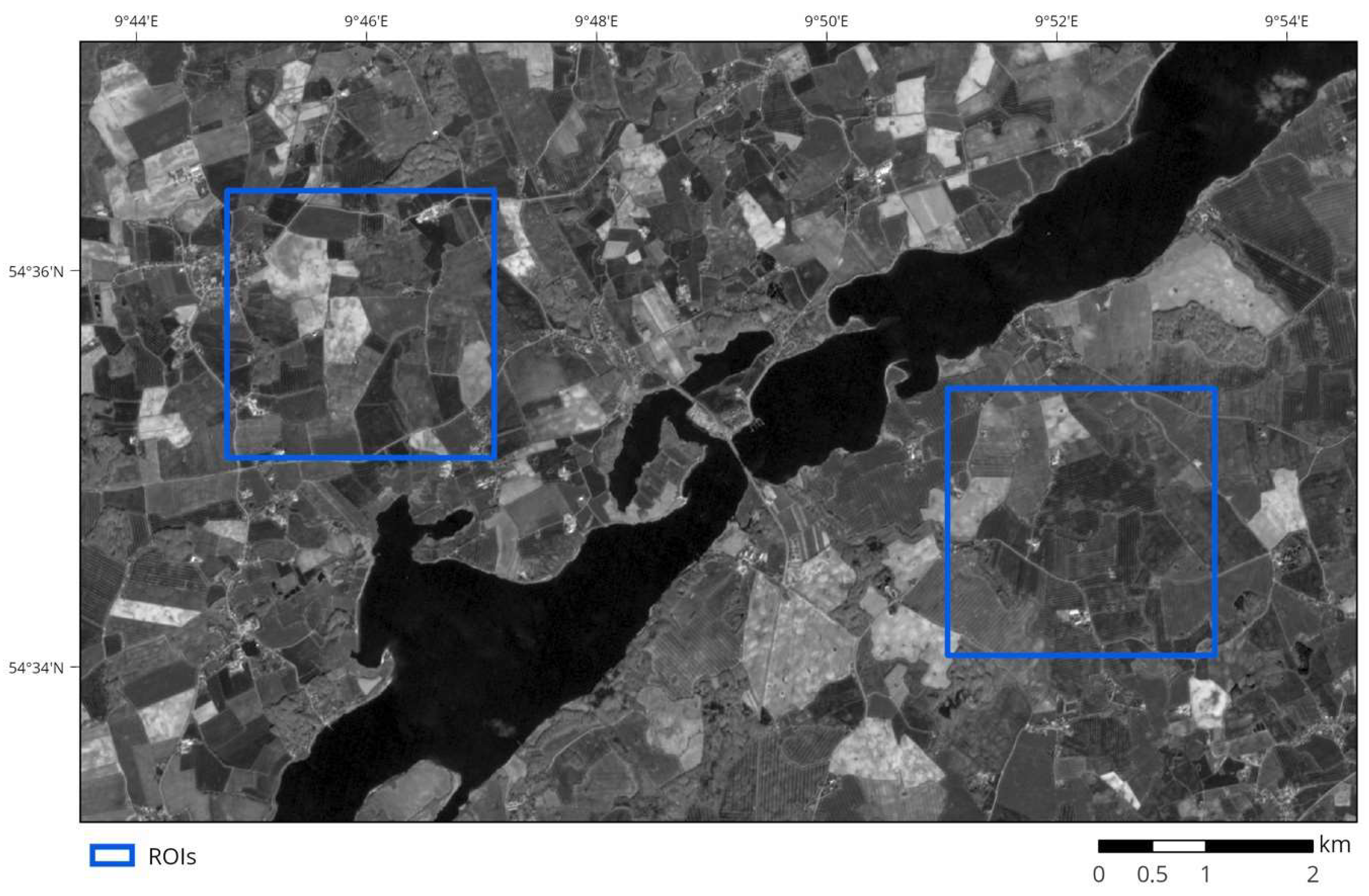
The region is dominated by agricultural use. It is rather heterogeneous with a mixture of small to mid-sized towns, forests, and agricultural areas with varying intensities of use. Farming in the region is highly industrialized and purely rain-fed. Main agricultural crops are cereals such as wheat, barley, and rye as well as maize and rapeseed [26]. Field shapes are irregular, with no predominant patterns. Field characteristics and distribution are heterogeneous, with sizes ranging from below 1 to above 10 ha. As seen in Figure 1, the landscape consists of a mixture of fields of different sizes and shapes. The whole study area had an extent of roughly 11.5 × 7.0 km². Within it, we selected two 2.5 × 2.5 km² regions of interest (ROIs) for detailed analysis (see Figure 1). We created a reference dataset for each of them representing all fields that should be extracted from the subset alone (i.e., all fields contained entirely within the subset).
2.2. Satellite Imagery
For our study, we used Sentinel-2 Level-2A atmospherically corrected imagery. To cover different growth stages and maximize the differentiation of neighboring fields (see Section 3.2), we explored scenes throughout the 2019 crop growing season (March until late October). Considering only observations without cloud cover over the study area, our dataset consisted of six scenes in March, April, June, July, August, and September. To provide sufficient spatial detail, we focused only on the 10-m-resolution red, green, and blue (RGB) bands of Sentinel-2. This further allows us to explore the potential applicability of our method to other sensors with a more limited selection of wavelength bands or even a standard RGB setup.
2.3. Reference Data
State cadastral data containing administrative plots served as a reference [27]. Although the boundaries in this dataset sometimes aligned with actual field boundaries of 2019, manual updating was required based on field surveys and recent satellite imagery. Considering that the 10 m spatial resolution of Sentinel-2 limited the capacity to extract very small plots, we excluded all polygons below a size of 0.5 ha.
Interpretation of field conditions proved difficult. On some occasions, fields appeared as separate at one point in time (e.g., due to separate tilling) but merged in later images. In other cases, the delineation of two adjacent plots was difficult (see also Section 5).
2.4. Land Cover Mask
As we were only interested in agricultural areas, we masked all non-agricultural landscapes using land cover maps. We considered two products: the CORINE land cover data of 2018 and the Land Cover DE product of the German Aerospace Center (DLR) [28,29]. Previous investigation demonstrated superior quality of the DLR product in our study area, but we still occasionally observed some urban and other non-agricultural areas as being misclassified. We therefore decided to use a combination of the two products to create a conservative land cover mask.
3. Methodology
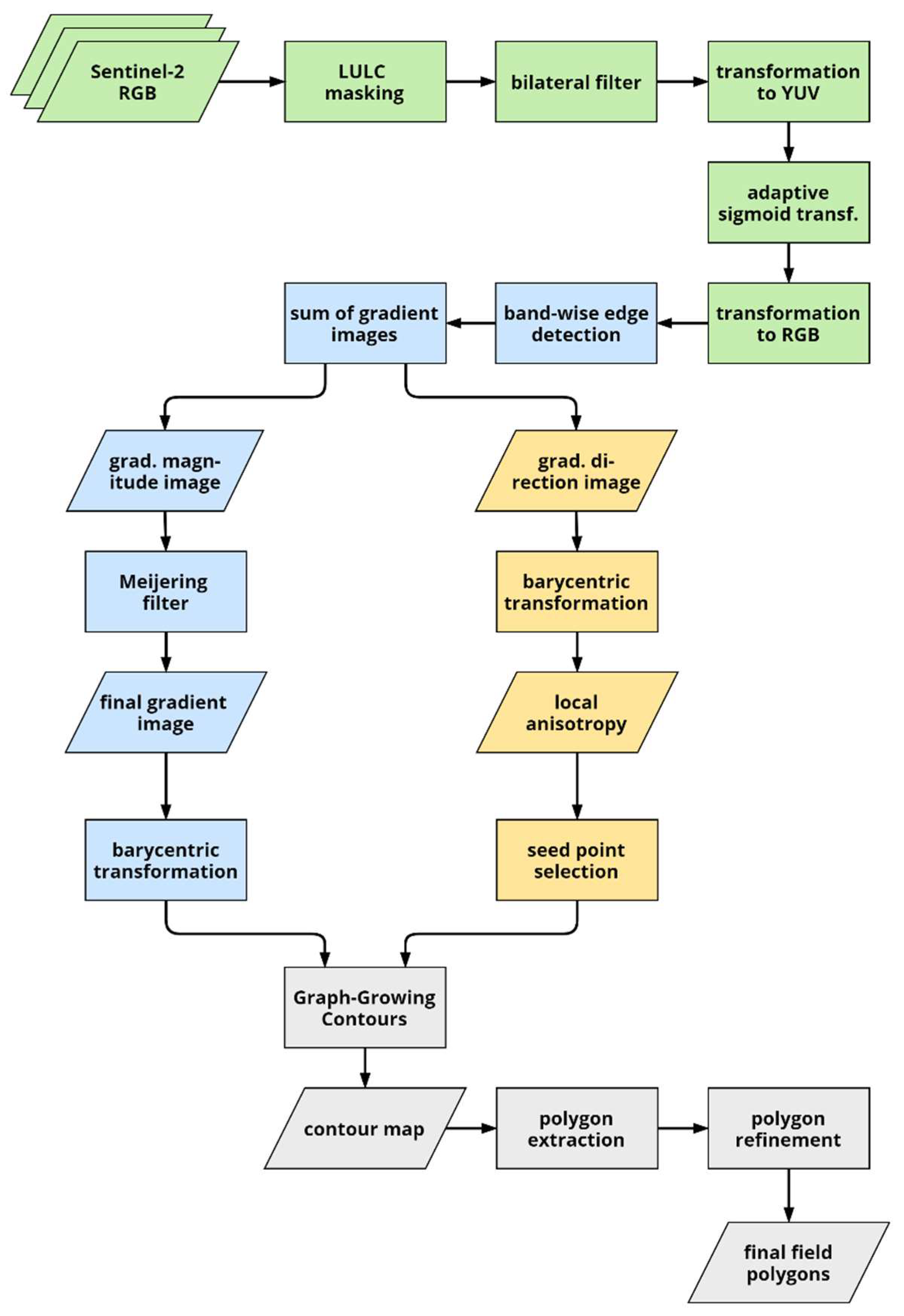
The flowchart in Figure 2 provides an overview of the workflow of our approach. After providing some background on pixel value transformation and active contours, we first describe the image pre-processing and enhancement (green) in Section 3.2, then proceed with the edge detection (blue) in Section 3.3 before describing seed point selection (yellow) as well as contour and polygon extraction in Section 3.4 and Section 3.5.
3.1. Background
3.1.1. Sub-Pixel Image Transform
To perform analyses on the sub-pixel level, we dynamically transformed the pixel grid data of the images using a barycentric transform, which represent the location of a point within a triangle (or more generally a simplex) as the center of mass (i.e., the barycenter) in relation to its vertices [30].
Barycentric coordinates have proved to be useful in finite element analysis and computer graphics applications, and are superior to simple distance-weighted transforms. To obtain the value of a given point, the three closest grid points in the image are selected as vertices of the triangle. The value is then computed as a linear combination of these vertices based on the following equations:
where , and denote the three vertices of the triangle, and are the x- and y-coordinates of the vertex , and and are the x- and y-coordinates of the interior point. , , and are the weights assigned to each vertex. As long as a point is located within the triangle, all three weights are ≥0 and sum up to 1.
3.1.2. Active Contours and Growing Snakes
Active contours (also called snakes) were first introduced by Kass et al. for object delineation [31]. The concept is based on the energy minimization of a deformable spline or polyline. The spline is initiated either via user input (e.g., a rough sketch around the object of interest) or automatically in the object’s vicinity. The snake then follows two influencing factors: the external and internal energy. The external energy given by the image (e.g., the gradient magnitude) directs the snake towards the contour of interest. The internal energy determines the shape of the snake and usually consists of two parts: continuity and smoothness or curvature, often represented by the first and second derivative. They limit the curvature of the contour and the distance between individual points. This ensures that the snake does not expand or contract indefinitely or become discontinuous. A traditional snake is described as a parametric curve , following the energy given by the equation below [31,32]:
where and describe the first and second derivatives of the parametric curve and and are weighting parameters that determine the influence on continuity (first derivative) and curvature (second derivative). is the external energy. One major drawback of the original model (and many subsequent variants for that matter) is the difficult choice of initial placement due to high sensitivity regarding initialization [33].
Many variants of the active contour model have been proposed to address various drawbacks or expand the model for use in new applications, including geodesic contours using level sets and various different external energies such as edge distance transform or gradient vector flow [32,34]. The aim of our use case was not to detect single objects, but rather to extract a complex network of contours that may not even be interconnected and conserve contour relationships. Given the irregular sizes and shapes of fields in our study area, it should further be independent of shape or size priors.
We therefore focused on the so-called growing snakes model introduced by Velasco and Marroquin, which was designed particularly for complex topologies where traditional active contours may struggle [33]. Growing contours are initialized on seed points along the contour itself and grow (or “move”) in steps perpendicular to the local gradient direction (i.e., along the contour). Movement in each step is determined by selecting the position of highest gradient magnitude out of a set of possible locations. The process proceeds until the snake approaches an existing contour point. In this case, the growth process stops, forming either a T-junction or a closed line. Although capable of tracking heterogeneous boundaries, this method simply follows local maxima. Therefore, it has a tendency to create discontinuous contours, as it does not consider the smoothness of the curve and requires an additional smoothing step.
We observed that growing contours had a tendency to get “off track” easily when the image gradient was heterogeneous, especially at corner points of multiple edges. Following the local maximum of gradient magnitude, the contour moves away from the actual boundary. Once this happens, it will create false boundaries along any local maxima it encounters. To address this, we experimented with user-defined constraints, for example, allowing only a certain number of steps with low magnitudes before terminating the snake. However, this introduced another level of complexity, as the threshold may be dependent on the strength of the edge currently being explored. If the snake is initiated on a very strong edge, a conservative threshold may ascertain good results; however, the process may stop prematurely if the explored edge is rather weak.
Another issue we encountered was the already mentioned tendency to produce discontinuous lines, either failing to represent sharp 90° turns and crossing edges or producing false turns. To avoid this, we limited the maximum amount of turns allowed and experimented with different movement schemes. Again, these modifications produced unreliable results and added complexity to the parameter settings. Hence, we developed a new graph-based growing contour model, described in Section 3.4.
3.2. Image Pre-Processing
The initial stage in our procedure is image pre-processing, serving multiple purposes: (a) removing non-agricultural areas; (b) reducing noise; (c) removing undesired effects due to sub-field features such as crop rows; and (d) enhancing actual field boundaries. The process comprised four parts. First, we mask non-agricultural areas based on the land use mask and created an RGB composite using bands 4, 3, and 2 of each scene. This particular band arrangement is not a prerequisite for further processing steps, and any three-band composite would suffice.
Second, we perform noise reduction and image smoothing. Particularly in edge detection, noise reduction is important to reduce the amount of spurious edges. In the context of this study, we define noise as any kind of non-boundary feature that may interfere with the boundary detection steps (e.g., soil and plant growth patterns). Although convolution of the image with a Gaussian kernel is a common approach, it has the negative side effect of blurring out potentially relevant edges as well. As we are particularly interested in edges corresponding to field boundaries, it is desirable to conserve stronger edges. To achieve this, we employ bilateral filtering. The bilateral filter combines a Gaussian distribution in the spatial domain (as regular Gaussian smoothing), defined by a standard deviation , with a Gaussian distribution in the value domain, defined by a standard deviation [35]. While the former determines the weighting of neighboring pixels based on their distance from the center pixel, the latter determines how values are weighted based on similarity to the center pixel. Edges in the image refer to sharp changes in image reflectance. Therefore, a smaller will conserve even weaker edges, while a larger will lead to a stronger blurring. The definition of the two distributions should be chosen carefully to ensure that weak, potentially irrelevant, edges are removed while strong edges are conserved.
Third, we transform the RGB image into the YUV color space. The YUV color space, similar to the closely related YCbCr color model, transforms the RGB information such that luminance is stored in the Y component while U and V refer to chrominance information. This enables image enhancement with reduced color information distortion. Fourth, we apply a sigmoid transform to the Y component to increase contrast of the image [36]. The sigmoidal function is defined as follows:
where is the reflectance of a pixel, is the slope of the sigmoidal curve (gain), and controls the centering of the sigmoid curve (offset).
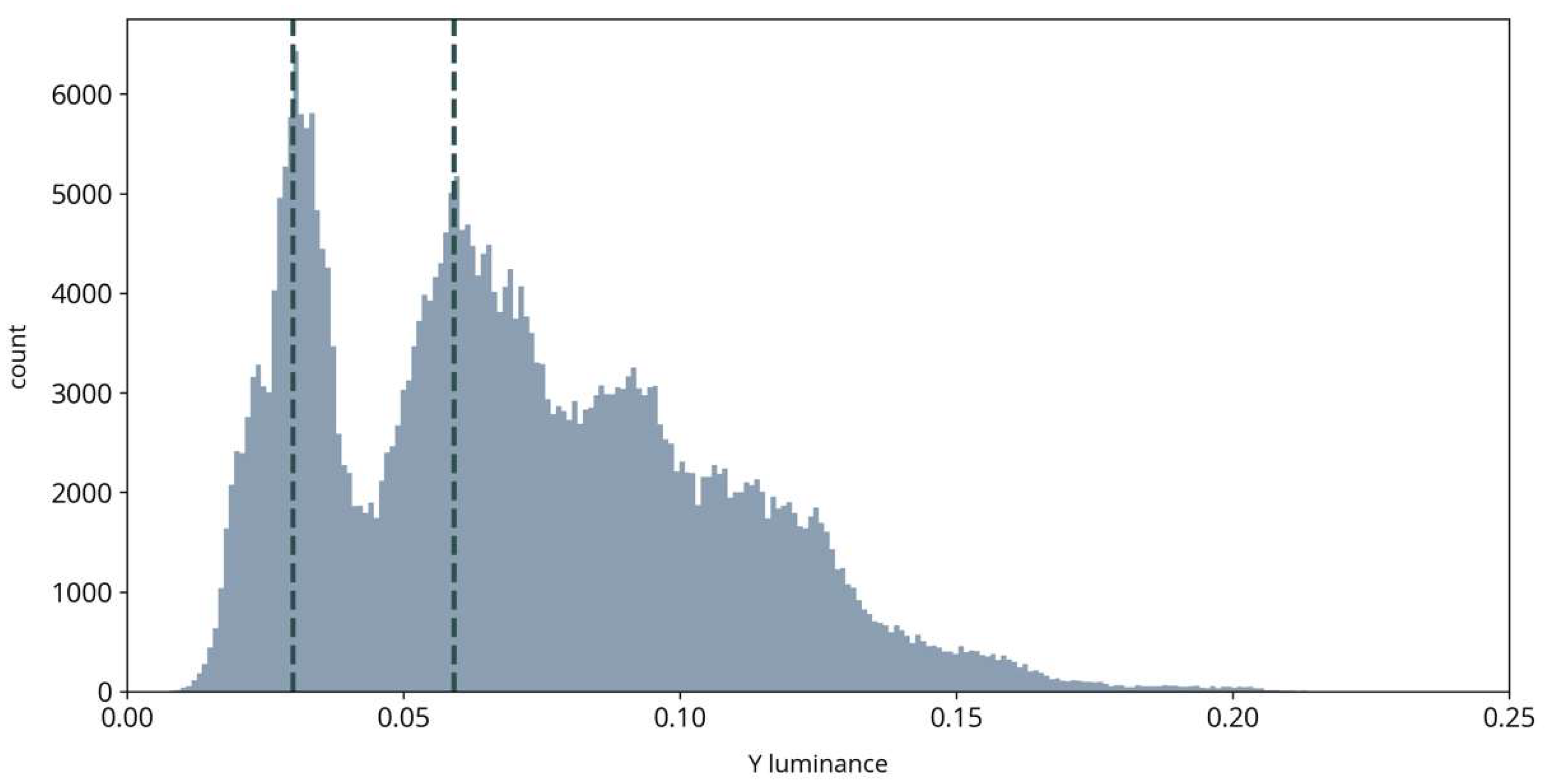
As illustrated in Figure 3, luminance images in our observations were usually bimodal, with the two peaks representing dark areas such as fully grown crops and bright areas such as dry open soil, respectively. The cutoff location of the sigmoid function can be adaptively positioned between the two peaks to increase contrast between dark and bright parts in the image. In the last step, we transform the YUV data back to RGB color space for subsequent steps.
3.3. Edge Detection and Enhancement
We convolve each of the three bands of each scene with the Sobel operator in both x- and y-directions:
We sum up the resulting gradient images to highlight recurring edges and use the summed horizontal and vertical gradient images to obtain overall gradient magnitude and gradient direction following the formulas:
where and are the gradient images in x- and y-directions.
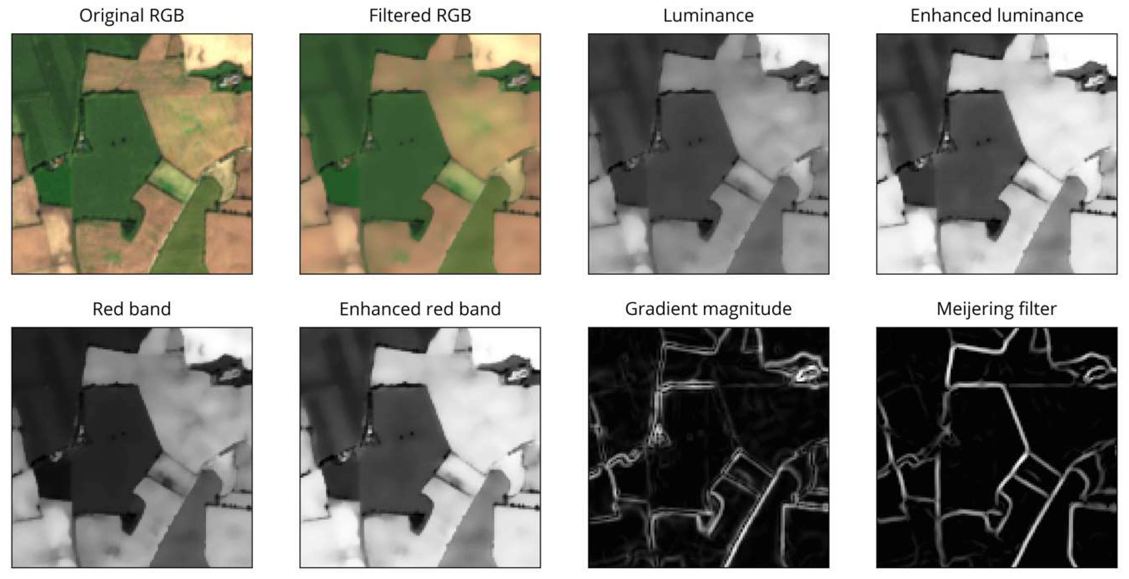
Despite smoothing, the gradient magnitude still contains spurious edges caused by crop rows and other features within some fields. Some of these edges are rather strong and consistent (appearing in multiple scenes) and could not be removed by filtering alone. To overcome this and further emphasize the actual field boundaries, we exploit the shape and appearance of boundaries by applying a Meijering filter to the magnitude image [37]. This filter was originally designed for medical purposes to extract neurites from microscopic images. It uses the eigenvectors and eigenvalues of the second-derivative (Hessian) matrix of the image to determine the “ridgeness” of a pixel. By applying this filter, we can exploit the curvilinear structure of the field boundaries in the image (see Figure 4).
As seen in Figure 4, many remaining spurious edges disappeared or were at least substantially reduced. Further, the Meijering filter provided a good representation of the actual contour shape compared to the sometimes uneven and blurred appearance of the gradient magnitude image. The resulting image was normalized and was the basis for most subsequent procedures, referred to as (gradient) magnitude.
3.4. Graph-Based Growing Contours
We overcome the limitations observed in the growing snakes model (see Section 3.1.2) with a newly developed modified growing contours model called graph-based growing contours (GGC). The goal of our GGC technique is not only to locate potential field boundaries but also to facilitate the extraction of the actual fields. The main improvement lies in a newly designed movement based on graph theory concepts. We aimed to address five goals: (a) improve the quality of extracted contours and reduce the need for repeated smoothing; (b) introduce adaptive behavior to accurately trace the contours of different shapes (smooth curves, sharp corners, straight lines etc.); (c) increase the capacity to extract complex, irregular networks with multiple crossing edges and T-junctions via automatic branching; (d) improve the handling of “dead ends”; (e) automatically create an interconnected network of contours rather than a set of separate segments.
Parts of this concept were inspired by the methodology by Aganj et al., who used a Hough transform and orientation distribution functions for fiber tracking in diffusion-weighted magnetic resonance images [38]. In a similar fashion, we employ principles of graph theory to extract the most likely boundary paths in a local neighborhood.
3.4.1. Seed Point Selection
The technique is rather flexible with respect to initialization, but ideally starts at one or multiple points on the boundaries of interest. In case of an interconnected network of boundaries, even a single initial seed point is often sufficient to extract all boundaries in the image. However, to ensure coverage over a larger area, multiple potential seeds are preferable. This also ensures that weakly connected parts of the boundaries are correctly extracted.
Our observations showed that initializing the method on individual seed points consecutively provided the best results. The process starts on one seed point and proceeds until termination before being re-initialized on the next seed point.
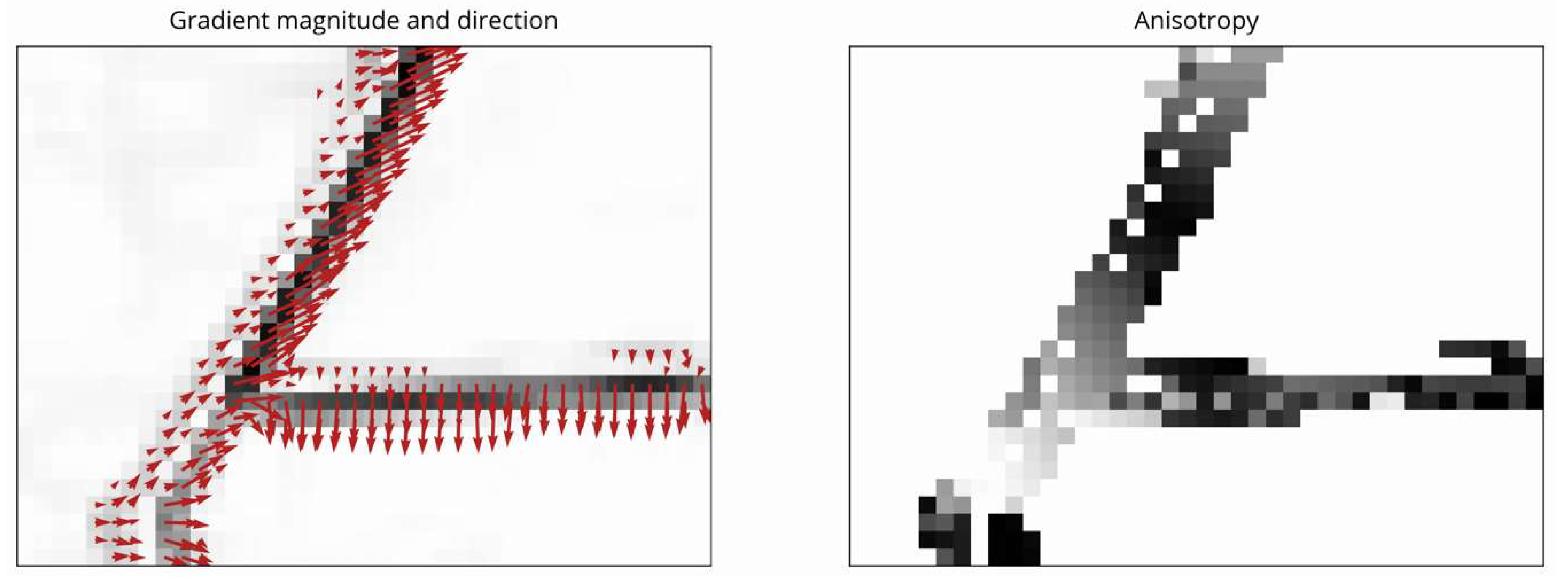
We therefore generate multiple seed points by selecting one point per 50 × 50 pixel image tile of the scene. For each tile, we limit the choice to those pixels located on strong edges. To determine potentially useful starting points, we assume that points near changing gradient direction such as corners or crossings of multiple edges are most suitable. These points allow the quick exploration of several branches and usually do not run the risk of producing only dead ends. As seen in Figure 5, regions along a single boundary are usually areas of similar gradient direction, while regions near corners, curves, and crossings contain gradients of different directions [39]. To transfer this to an easy-to-use metric, we approximate the local anisotropy. Isotropy is defined as being direction-invariant [40]. Following this definition, pixels along edges are more anisotropic (low isotropy), while those near corners and crossings of multiple boundaries are less anisotropic (high isotropy).
We approximate local anisotropy by sampling the gradient direction in a pattern around each pixel (similar to Section 3.4.2). We then determine the predominant or primary gradient direction by assigning the vectors to 16 bins between and . The bin containing the largest number of vectors defines the predominant direction. We then project all vectors onto the main directional unit vector as well as the unit vector normal to it. We calculate the total magnitude of projected vectors in both directions and obtain anisotropy via:
where and are the main directional and normal vectors, respectively, describes a given local gradient direction vector, and is the number of all sampled vectors. If the total magnitude in both directions is similar, anisotropy is low. If the magnitude in one direction is much larger than the other, we observe a high anisotropy (see Figure 5). This information is used to select points of high isotropy as seed points.
3.4.2. Generating a Local Graph
At each end point, the model starts by creating a directed, weighted graph. Firstly, a set of points around the end point is sampled on the sub-pixel level using a concentric circular pattern, as seen in Figure 6. The pattern is defined by an inner radius , an outer radius , the number of points on the initial (innermost) circle , and the number of evenly spaced circles . Moving outwards, the number of points doubles with each circle, creating a homogeneous pattern. This ensures that each point on a circle has the same number of neighbors on the next circle. As seen in Figure 6, the pattern also ensures straight connections from each point of the inner circle to the outermost one.
The sampled points represent nodes in a local directed, unweighted graph constructed based on a set of rules:
- The center point and all sampled points are nodes in the graph.
- The center node is linked via edges to all nodes of the initial circle with equal weights.
- Each subsequent node is connected to the same number of nearest nodes on the next larger circle via directed, outgoing edges .
- In the direction of the previous contour location, nodes of the graph are masked to avoid backtracking.
All edges (except the ones originating at the center) are weighted based on:
where is the weight of the edge , is the Euclidian distance between the nodes and , and is the gradient magnitude at node . This weighting allows for consideration of both distance between the points (favoring shorter paths in terms of Euclidian distance) and regions of higher magnitude (favoring locations along an edge in the image).
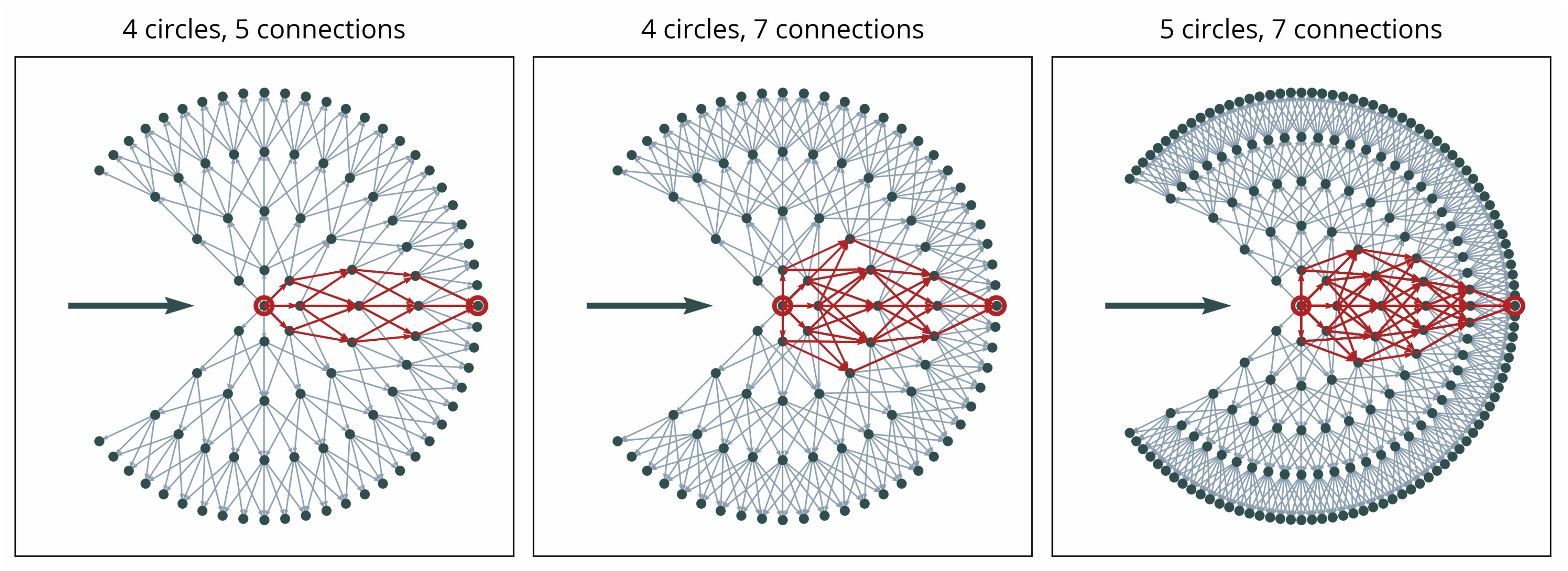
In constructing the graph, may be regarded as a metric of accuracy or smoothness because, given the same radius, more points will tend to create smoother curves (see Figure 7). Similarly, the number of allowed connections from each point to the next circle will influence both the smoothness and the capacity for sharper directional changes (see Figure 7). We presume the number of points on the initial circle as a parameter of potential directionality, which may influence the capacity to consider different directions. The parameter may be regarded as a “step size”.
As illustrated in Figure 7, different paths may lead to each point along the outer circle. This ensures the capacity to represent different shapes of contours, including sharp corners or smooth curvatures. However, the distance component in the weighting Equation (13) ensures that smoother curves are preferred. The complexity of the graph and, as a result, processing time, increase with larger values of , , and .
3.4.3. Movement
To determine the branches (i.e., directions of movement) at a current point, a shortest-path search starting at the center node (source) of the local graph to all nodes of the outermost circle (sinks) is initiated using Dijkstra’s algorithm [41]. There are various potential ways of deciding subsequent directions. One may simply search for local minima or select a certain number of shortest paths. However, boundary features in the image usually expand over multiple end nodes on the circle. This may lead to multiple selected paths corresponding to the same image feature while other less-pronounced features remain unconsidered.
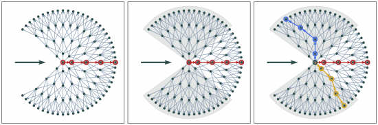
To avoid this, we first select the overall shortest path as the first branch. We take the location of the first path as a reference and split the graph into subsections around and from the main direction. Subsequent paths are selected only within these sections of the graph. The shortest paths in each of the sections are selected as potential branches (see Figure 8, right panel). If there are two edges branching at a very small angle, the two boundary features usually diverge quickly. This can still be represented in the graph (see Figure 8, right panel).
Any selected paths that are longer than a certain threshold are omitted. This ensures superfluous branches to die off quickly rather than continuing indefinitely and leads to a dynamically changing number of end points and automatic termination of “dead ends”.
An end point of the contour is terminated if no valid paths are found, if the current point is near the image boundaries, or if it is near an already existing contour point. In the latter case, the two points are connected.
3.5. Polygon Creation and Post-Processing
The output of GGC is a large undirected network (graph) of interconnected contour points. The next challenge is to transform this network of field boundaries into a set of individual field polygons. Simple clustering or associating points with certain shapes in the image are unreliable because points are usually part of multiple neighboring fields, and field shapes may be quite heterogeneous. We did not intend to introduce any assumptions about field shapes or contour arrangements.
Again, we make use of graph theory concepts. In theory, this is as simple as finding cycles in the graph, but in practice some problems may arise. On the one hand, the network may become very large, especially if small step sizes are used (i.e., small ), making the process of detecting cycles computationally demanding. On the other hand, the process requires a correctly interconnected network with no false edges or gaps.
To improve performance and increase reliability, we decided to create local polygons using a subset of boundary points. To achieve this, we transform the set of edges in the output graph to a binary contour image by drawing a binary edge map. We then employ a flood fill algorithm creating a segment representing the rough extent of a given field as defined by the extracted contours. Then, we extract the nodes of the network located within a certain distance from the boundary pixels of the flood fill segment. A new field boundary graph is created where each node is connected to its four nearest neighbors. This may produce an over-connected graph. The polygon representing the field is extracted by finding the longest cycle in this local network. To refine the polygons, we further employ adaptive Gaussian filtering and the Ramer–Douglas–Peucker algorithm [42,43,44].
3.6. Selecting Optimal Parameters
The pre-processing steps are particularly crucial for the performance of our approach, especially the correct filtering of the images. Regarding the parameters of the GGC model, we decided to set constant values for many of them to reduce complexity of the optimization task. In the two ROIs, we chose four parameters for optimization to obtain representative results: the two standard deviations defining bilateral filtering and , the gain in the sigmoid transformation, and the maximum allowed path length in GGC. For other settings we found = 8, = 6, and = 7 to be good default values in both ROIs.
We obtained an optimum parameter setting for both ROIs using differential evolution in a “rand-best/1/bin” strategy with a population size of 20, differential weight of 0.3, and crossover rate of 0.8 [45,46]. We visually compared the obtained extraction results to a representative image and the reference datasets. The target variable of optimization was the mean Jaccard index (see Section 3.7). In both ROIs, the differential evolution converged within 20 iterations and determined an optimal parameter set as given in Table 1. Optimal settings for both ROIs were overall similar in terms of a quite large difference between and and relatively high values of .
3.7. Performance Evaluation
We used a quantitative metric to evaluate the difference between extracted polygons and those in the reference set. We employed the frequently used Jaccard Index as our main reference metric because it is a common metric performing well for automatic segmentation [47]. In a pre-cursor step, extracted and reference polygons need to be matched [47]. Considering the set of reference polygons and the set of extracted polygons , we can define multiple subsets. Following Clinton et al. [48], we can distinguish:
Resulting values range from 0 to 1, with 0 indicating an optimal segmentation. If the set of matched polygons is empty, is set to 1. All values calculated for individual polygons were averaged. In addition, we used statistical information in the form of the number of fields, median and standard deviation of field sizes, and total acreage as proxies for performance of field extraction. We focused our detailed analysis on the two ROIs but also briefly discuss the performance on the whole study area using both parameter settings.
4. Results
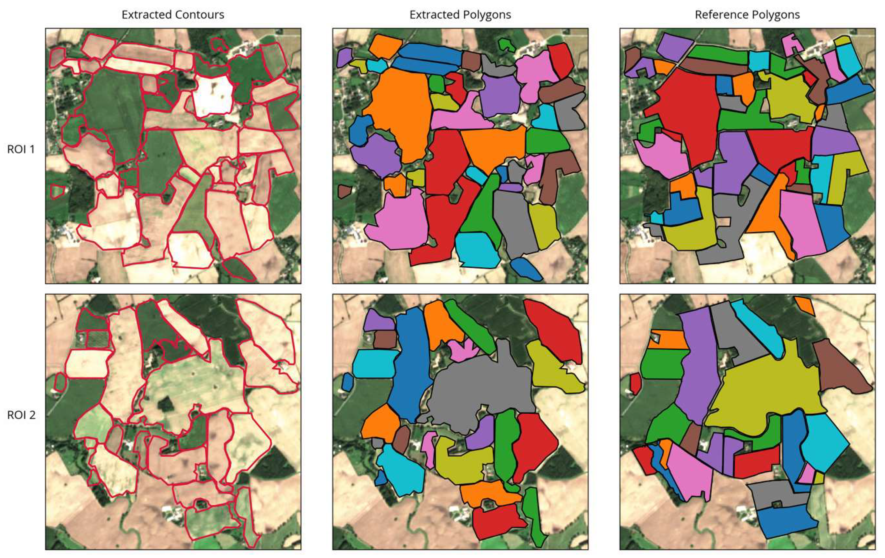
As shown in Figure 9, the overall appearance of the extraction results in both ROIs was close to a visual interpretation of the image. The general arrangement of extracted fields was matched and most shapes were correctly delineated, closely following the visible boundaries in the images. Spatially isolated phenomena such as patches of wet soil, grass growing within bare fields, or uneven growth stages within a field did not confuse the extraction as long as they were located at some distance from the field boundaries (see Figure 9, fields near the top of ROI 1 and at the center-right in ROI 2). However, if they were located close to or directly on a boundary, they could cause irregular field shapes or incorrect indents in the outline (e.g., Figure 9, ROI 2 center).
Uncertainties may also occur in case of temporally isolated distinctions, for example, when adjacent fields are only distinguishable at a specific point in time but remain homogeneous otherwise. Our approach was successful in detecting field boundaries, even if they were just visible in a single image. For example, the two elongated fields in the top left in ROI 1 appear to be one large field in all but the one observation pictured, where only the northern half is ploughed (see Figure 9). In such cases, the strength of the delineating features is crucial (Section 5).
The method further detected some additional fields near the boundaries of the image that were not part of the reference dataset. This was due to the actual fields extending slightly outside the ROI, while the extraction still detected a large portion of the field.
Table 2 presents the statistics for the two ROIs. In general, results were close to those of the reference datasets. The total acreage of all fields showed a high agreement for both ROIs. Median field sizes in the two ROIs were quite different, with ROI 1 containing mostly smaller fields (median size 5.08 ha in the reference data) than ROI 2 (median size of 8.67 ha). Delineated field contours and sizes in ROI 1 matched accurately with a difference in median field size of just 0.52 ha. In ROI 2, however, the offset in median field size was more significant (1.39 ha). The number of fields extracted was off by -4 and +2 in ROIs 1 and 2, respectively. This was due to some larger fields being mistaken for two separate plots or vice versa, as well as the above-mentioned extraction of additional fields near the image boundaries.
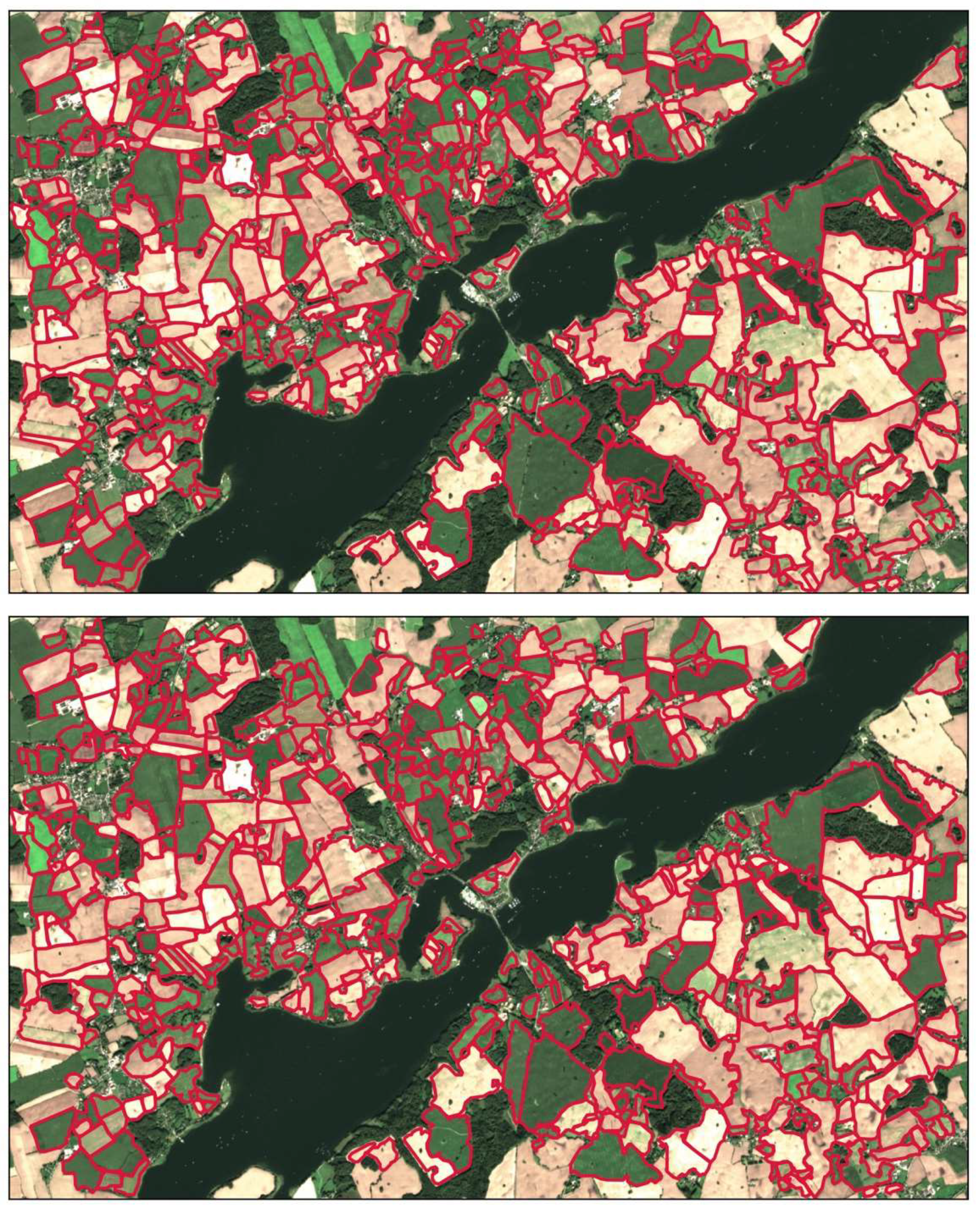
Results on the whole study area are shown in Figure 10 for both parameter setups. Both showed mixed results. In some areas (especially near the respective ROIs), results were good but performance deteriorated further away from the regions for which the settings were optimized.
5. Discussion
The presented GGC method proved reliable in extracting complex networks of boundaries with minimal supervision. Once initiated, it automatically detected relevant boundaries in the image, often only requiring a single seed point. Automatic branching at diverging or crossing edges worked reliably, and “dead ends” (i.e., undesired branches following spurious edges) were avoided for the most part. This ensured the successful extraction of many of the irregularly shaped fields in the reference data.
The field extraction approach produced good results in terms of statistical characteristics of the field structure in the two ROIs. The total acreage was matched very closely. Overall, ROI 2 proved more challenging than ROI 1, possibly due to a more heterogeneous appearance because of wet soils and uneven growth patterns. This became apparent in the overestimated median field size. The total number of fields extracted in the two ROIs also reflected some issues. The algorithm missed some very small fields, while merging some larger, heterogeneous ones. However, as mentioned before, interpretation of actually separated fields vs. separately managed parts of one larger field is difficult, and may explain some of these issues.
The proposed method further proved reliable in extracting even narrow field strips and many smaller plots, but was occasionally confused by inconsistencies near urban areas or single man-made structures. This may be addressed through better masking of undesired objects, but would require much better knowledge of conditions in the area or significantly more pre-processing time. For such cases, further research is needed to ensure higher reliability.
We also observed uncertainties regarding temporally confined features like temporarily wet soils or field management, which can introduce heterogeneities within a single field. In such cases, delineation is may be ambiguous. In part, the use of multi-temporal data sets helped to enhance weaker but consistent field boundaries. In most cases, our technique was capable of detecting weak but consistent boundaries. Problems occurred, however, if the separation only appeared in a single observation: if the boundary is pronounced, the algorithm is capable of correctly delineating the fields, even if a separation is only visible in one observation. However, if groups of adjacent fields are separated by a weak border, they may be detected as a single large field (see Figure 9, ROI 1 bottom left). The point at which different appearances or spatially or temporally constrained boundaries actually justify a separation into multiple fields is debatable. However, by adjusting , the user can influence the degree to which the model considers weaker boundaries. Since there is a trade-off between detecting weak boundaries and reducing the risk of extracting false boundaries, more research is needed to address this issue—for example, by adapting pre-processing steps such as contrast stretching or edge detection to the individual images or by introducing a dynamic weighting.
Overall, we observed that the pre-processing had the greatest influence on the performance of the whole process. The filtering and edge enhancement steps we employed proved for the most part effective in reducing background noise and highlighting actual field boundaries. Especially, the use of multi-temporal Sentinel-2 data to emphasize weaker structures and the Meijering filter to reduce spurious edges proved useful. In general, the better the prior boundary detection step, the more reliable and efficient the GGC contour extraction process can be. With a more reliable and homogeneous input, a larger radius can be chosen without the need to increase the number of circles too much. This would speed up the process and reduce the number of iterations required.
The spatial resolution of Sentinel-2 also limits the approach. Although 10 m resolution is sufficient in most cases, it may hamper the precise extraction of very small fields. Overall, we found the spatial resolution to be suitable for this task, but we expect that higher resolutions would provide better results. We would further speculate the “sweet spot” resolution to be between 1 and 5 m for this type of application. At this scale, delineation would become even more accurate and would make it possible to distinguish smaller objects such as single man-made structures, narrow hedges, or trees. However, with sub-meter resolutions, separating meaningful information from “noise” like soil texture or individual plants may become difficult. Moreover, processing time would increase dramatically and the benefit from additional detail would probably not outweigh the drawbacks. Future research may explore the performance of our technique on higher-resolution imagery.
It became apparent that different parameter settings are required for reliable field extraction in the two ROIs, in both the pre-processing and the actual extraction steps. This was particularly obvious in applications to the whole study area, and may have been aggravated by the heterogeneous structure of the agricultural landscape. Different circumstances in different parts of the region led to inconsistent results when using the same settings for the entire area. As mentioned previously, this was mainly due to different requirements in the boundary detection step. In the future, it would be desirable to explore an adaptive procedure that chooses parameters based on characteristics such as structure, morphology, and statistics of the input imagery. Judging from the results of this study, subsets even smaller than 2.5 × 2.5 km² may be advantageous to allow local adaptations, even at field scales.
As mentioned above, further improvements to the algorithm may also include pre-processing and boundary detection steps. Considering not only different scene characteristics but also the date of image acquisition in a time series may improve delineation results, for example, via dynamic image filtering and enhancement procedures depending on the characteristics of individual images. Further, analysis of image stacks may be employed to dynamically select desirable features (e.g., by giving higher weights to images with more pronounced boundary features). The polygon refinement may also be adapted to criteria such as predominant field shapes and required detail.
It is also desirable to ensure that higher values of do not result in more dead ends along extracted boundaries but only prolong movement along relevant but weak boundaries.
6. Conclusions
We presented a new method for field boundary detection and subsequent field polygon extraction based on image enhancement, edge detection, and a new version of the growing snakes active contours model called graph-growing contours. The approach succeeded in extracting field boundaries on the sub-pixel level from a set of Sentinel-2 RGB images. The method is very flexible in its application, as it is not restricted to imagery of a certain sensor, resolution, or wavelength, but can utilize any combination of bands as an RGB input. The boundary extraction step using the new GGC model also requires little supervision. Once initialized, it automatically extracts even large networks of complex interconnected boundaries.
There were some issues with respect to weak field boundaries, urban structures, or temporary disturbances such as wet soil patches in fields. However, most of these are probably best addressed in the pre-processing steps and are not inherent flaws of the extraction procedure. The flexibility of the presented contour extraction allows the use of any kind of image-like data representing field boundaries. The polygon extraction method may therefore be used in combination with other field boundary detection algorithms.
We are currently exploring the potential to improve the process with respect to small-scale image features, inconsistencies at edges, and better highlighting of relevant vs. irrelevant boundary features. Further, we plan to generalize and scale up the extraction procedure to larger areas—possibly even landscape scales. This may require further work regarding automatic adaptation to local conditions and available imagery or improvements to the boundary detection step.
Author Contributions
The concept and design of the study were conceived by M.P.W. in collaboration with N.O. Methodology design, implementation, optimization, and analysis of results were carried out by M.P.W. M.P.W. wrote the majority of the manuscript, with N.O. contributing in reviewing and finalizing the manuscript. All authors have read and agreed to the published version of the manuscript.
Funding
Financial support for publication fees was provided by Land Schleswig-Holstein within the funding programme Open Access Publikationsfonds.
Acknowledgments
We thank the students and student assistants who carried out in-situ mapping campaigns and helped to produce and update the reference data.
Conflicts of Interest
The authors declare no conflict of interest.
References
- Graesser, J.; Ramankutty, N. Detection of cropland field parcels from Landsat imagery. Remote Sens. Environ. 2017, 201, 165–180. [Google Scholar] [CrossRef] [Green Version]
- Tilman, D.; Fargione, J.; Wolff, B.; D’Antonio, C.; Dobson, A.; Howarth, R.; Schindler, D.; Schlesinger, W.H.; Simberloff, D.; Swackhamer, D. Forecasting agriculturally driven global environmental change. Science (80-.) 2001, 292, 281–284. [Google Scholar] [CrossRef] [PubMed] [Green Version]
- Barrett, C.B.; Barbier, E.B.; Reardon, T. Agroindustrialization, globalization, and international development: The environmental implications. Environ. Dev. Econ. 2001, 6, 419–433. [Google Scholar] [CrossRef]
- García-Pedrero, A.; Gonzalo-Martín, C.; Lillo-Saavedra, M. A machine learning approach for agricultural parcel delineation through agglomerative segmentation. Int. J. Remote Sens. 2017, 38, 1809–1819. [Google Scholar] [CrossRef] [Green Version]
- European Court of Auditors. The Land Parcel Identification System A Useful Tool to Determine the Eligibility of Agricultural Land—But Its Management Could Be Further Improved; European Union: Luxembourg, 2016; ISBN 9789287259677. [Google Scholar]
- Sagris, V.; Devos, W. LPIS Core Conceptual Model: Methodology for Feature Catalogue and Application Schema; European Commission: Luxembourg, 2008. [Google Scholar]
- Inan, H.I.; Sagris, V.; Devos, W.; Milenov, P.; van Oosterom, P.; Zevenbergen, J. Data model for the collaboration between land administration systems and agricultural land parcel identification systems. J. Environ. Manag. 2010, 91, 2440–2454. [Google Scholar] [CrossRef] [PubMed] [Green Version]
- Tiwari, P.S.; Pande, H.; Kumar, M.; Dadhwal, V.K. Potential of IRS P-6 LISS IV for agriculture field boundary delineation. J. Appl. Remote Sens. 2009, 3, 033528. [Google Scholar] [CrossRef]
- Rahman, M.S.; Di, L.; Yu, Z.; Yu, E.G.; Tang, J.; Lin, L.; Zhang, C.; Gaigalas, J. Crop Field Boundary Delineation using Historical Crop Rotation Pattern. In Proceedings of the 2019 8th International Conference on Agro-Geoinformatics (Agro-Geoinformatics), Istanbul, Turkey, 16–19 July 2019; pp. 1–5. [Google Scholar] [CrossRef]
- Da Costa, J.P.; Michelet, F.; Germain, C.; Lavialle, O.; Grenier, G. Delineation of vine parcels by segmentation of high resolution remote sensed images. Precis. Agric. 2007, 8, 95–110. [Google Scholar] [CrossRef]
- Turker, M.; Kok, E.H. Field-based sub-boundary extraction from remote sensing imagery using perceptual grouping. ISPRS J. Photogramm. Remote Sens. 2013, 79, 106–121. [Google Scholar] [CrossRef]
- Yan, L.; Roy, D.P. Conterminous United States crop field size quantification from multi-temporal Landsat data. Remote Sens. Environ. 2016, 172, 67–86. [Google Scholar] [CrossRef] [Green Version]
- Rydberg, A.; Borgefors, G. Integrated method for boundary delineation of agricultural fields in multispectral satellite images. IEEE Trans. Geosci. Remote Sens. 2001, 39, 2514–2520. [Google Scholar] [CrossRef]
- Watkins, B.; van Niekerk, A. A comparison of object-based image analysis approaches for field boundary delineation using multi-temporal Sentinel-2 imagery. Comput. Electron. Agric. 2019, 158, 294–302. [Google Scholar] [CrossRef]
- Gonzalo-Martín, C.; Lillo-Saavedra, M.; Menasalvas, E.; Fonseca-Luengo, D.; García-Pedrero, A.; Costumero, R. Local optimal scale in a hierarchical segmentation method for satellite images: An OBIA approach for the agricultural landscape. J. Intell. Inf. Syst. 2016, 46, 517–529. [Google Scholar] [CrossRef] [Green Version]
- MacDonald, R.B.; Hall, F.G. Global crop forecasting. Science (80-.) 1980, 208, 670–679. [Google Scholar] [CrossRef]
- Atzberger, C. Advances in remote sensing of agriculture: Context description, existing operational monitoring systems and major information needs. Remote Sens. 2013, 5, 949–981. [Google Scholar] [CrossRef] [Green Version]
- Mulla, D.J. Twenty five years of remote sensing in precision agriculture: Key advances and remaining knowledge gaps. Biosyst. Eng. 2013, 114, 358–371. [Google Scholar] [CrossRef]
- Dorigo, W.A.; Zurita-Milla, R.; de Wit, A.J.W.; Brazile, J.; Singh, R.; Schaepman, M.E. A review on reflective remote sensing and data assimilation techniques for enhanced agroecosystem modeling. Int. J. Appl. Earth Obs. Geoinf. 2007, 9, 165–193. [Google Scholar] [CrossRef]
- Borgogno Mondino, E.; Corvino, G. Land tessellation effects in mapping agricultural areas by remote sensing at field level. Int. J. Remote Sens. 2019, 40, 7272–7286. [Google Scholar] [CrossRef]
- Yan, L.; Roy, D.P. Automated crop field extraction from multi-temporal Web Enabled Landsat Data. Remote Sens. Environ. 2014, 144, 42–64. [Google Scholar] [CrossRef] [Green Version]
- Debats, S.R.; Luo, D.; Estes, L.D.; Fuchs, T.J.; Caylor, K.K. A generalized computer vision approach to mapping crop fields in heterogeneous agricultural landscapes. Remote Sens. Environ. 2016, 179, 210–221. [Google Scholar] [CrossRef] [Green Version]
- Masoud, K.M.; Persello, C.; Tolpekin, V.A. Delineation of Agricultural Field Boundaries from Sentinel-2 Images Using a Novel Super-Resolution Contour Detector Based on Fully Convolutional Networks. Remote Sens. 2019, 12, 59. [Google Scholar] [CrossRef] [Green Version]
- Kottek, M.; Grieser, J.; Beck, C.; Rudolf, B.; Rubel, F. World Map of the Köppen-Geiger climate classification updated. Meteorol. Z. 2006, 15, 259–263. [Google Scholar] [CrossRef]
- Bundesanstalt für Geowissenschaften und Rohstoffe (BGR). Bodenübersichtskarte der Bundesrepublik Deutschland 1:200000 2018; Bundesanstalt für Geowissenschaften und Rohstoffe (BGR): Hannover, Germany, 2018. [Google Scholar]
- Ministerium für Energiewende, Landwirtschaft, Umwelt, N. und D. S.-H. Nutzung des landwirtschaftlichen Bodens—Schleswig-Holstein. Available online: http://www.umweltdaten.landsh.de/agrar/bericht/ar_tab_anz.php?ar_tab_zr_spalten.php?nseite=57&ntabnr=1%7C%7Car_tab_zr_spalten.php?nseite=57&ntabnr=3&Ref=GSB (accessed on 8 February 2020).
- Arbeitsgemeinschaft der Vermessungsverwaltungen der Länder der Bundesrepublik Deutschland (AdV). Produktspezifikation für ALKIS-Daten im Format Shape; Arbeitsgemeinschaft der Vermessungsverwaltungen der Länder der Bundesrepublik Deutschland (AdV): München, Germany, 2016. [Google Scholar]
- Weigand, M.; Staab, J.; Wurm, M.; Taubenböck, H. Spatial and semantic e ff ects of LUCAS samples on fully automated land use / land cover classi fi cation in high-resolution Sentinel-2 data. Int. J. Appl. Earth Obs Geoinf. 2020, 88, 102065. [Google Scholar] [CrossRef]
- Büttner, G.; Kosztra, B.; Soukup, T.; Sousa, A.; Langanke, T. CLC2018 Technical Guidelines; European Environment Agency: Vienna, Austria, 2017. [Google Scholar]
- Yiu, P. The uses of homogeneous barycentric coordinates in plane Euclidean geometry. Int. J. Math. Educ. Sci. Technol. 2000, 31, 569–578. [Google Scholar] [CrossRef]
- Kass, M.; Witkin, A.; Terzopoulos, D. Snakes: Active contour models. Int. J. Comput. Vis. 1988, 1, 321–331. [Google Scholar] [CrossRef]
- Xu, C.; Prince, J.L. Snakes, shapes, and gradient vector flow. IEEE Trans. Image Process. 1998, 7, 359–369. [Google Scholar] [CrossRef] [Green Version]
- Velasco, F.A.; Marroquin, J.L. Growing snakes: Active contours for complex topologies. Pattern Recognit. 2003, 36, 475–482. [Google Scholar] [CrossRef]
- Caselles, V.; Kimmel, R.; Sapiro, G. Geodesic Active Contours. Int. J. Comput. Vis. 1997, 22, 61–79. [Google Scholar] [CrossRef]
- Tomasi, C.; Manduchi, R. Bilateral filtering for gray and color images. Proc. IEEE Int. Conf. Comput. Vis. 1998, 839–846. [Google Scholar] [CrossRef]
- Braun, G.J.; Fairchild, M.D. Image Lightness Rescaling Using Sigmoidal Contrast Enhancement Functions. In Proc. SPIE 3648, Color Imaging: Device-Independent Color, Color Hardcopy, and Graphic Arts IV, Dec 22; SPIE: Washington, DC, USA, 1998; pp. 96–107. [Google Scholar]
- Meijering, E.; Jacob, M.; Sarria, J.-C.F.; Steiner, P.; Hirling, H.; Unser, M. Design and validation of a tool for neurite tracing and analysis in fluorescence microscopy images. Cytometry 2004, 58A, 167–176. [Google Scholar] [CrossRef] [Green Version]
- Aganj, I.; Lenglet, C.; Jahanshad, N.; Yacoub, E.; Harel, N.; Thompson, P.M.; Sapiro, G. A Hough transform global probabilistic approach to multiple-subject diffusion MRI tractography. Med. Image Anal. 2011, 15, 414–425. [Google Scholar] [CrossRef]
- Gregson, P.H. Using Angular Dispersion of Gradient Direction for Detecting Edge Ribbons. IEEE Trans. Pattern Anal. Mach. Intell. 1993, 15, 682–696. [Google Scholar] [CrossRef]
- Perona, P.; Malik, J. Scale Space and Edge Detection Using Anisotropic Diffusion. IEEE Trans. Pattern Anal. Mach. Intell. 1990, 12, 629–639. [Google Scholar] [CrossRef] [Green Version]
- Dijkstra, E.W. A note on two problems in connexion with graphs. Numer. Math. 1959, 1, 269–271. [Google Scholar] [CrossRef] [Green Version]
- Deng, G.; Cahill, L.W. An Adaptive Gaussian Filter For Noise Reduction and Edge Detection. In IEEE Conference Record Nuclear Science Symposium and Medical Imaging Conference, Oct 31–Nov 6; IEEE: San Francisco, CA, USA, 1993; pp. 1615–1619. [Google Scholar]
- Ramer, U. An iterative procedure for the polygonal approximation of plane curves. Comput. Graph. Image Process. 1972, 1, 244–256. [Google Scholar] [CrossRef]
- Douglas, D.H.; Peucker, T.K. Algorithms for the Reduction of the Number of Points Required To Represent a Digitized Line or Its Caricature. Cartogr. Int. J. Geogr. Inf. Geovisualization 1973, 10, 112–122. [Google Scholar] [CrossRef] [Green Version]
- Das, S.; Suganthan, P.N. Differential evolution: A survey of the state-of-the-art. IEEE Trans. Evol. Comput. 2011, 15, 4–31. [Google Scholar] [CrossRef]
- Charalampakis, A.E.; Dimou, C.K. Comparison of evolutionary algorithms for the identification of bouc-wen hysteretic systems. J. Comput. Civ. Eng. 2015, 29, 1–11. [Google Scholar] [CrossRef]
- Jozdani, S.; Chen, D. On the versatility of popular and recently proposed supervised evaluation metrics for segmentation quality of remotely sensed images: An experimental case study of building extraction. ISPRS J. Photogramm. Remote Sens. 2020, 160, 275–290. [Google Scholar] [CrossRef]
- Clinton, N.; Holt, A.; Scarborough, J.; Yan, L.I.; Gong, P. Accuracy assessment measures for object-based image segmentation goodness. Photogramm. Eng. Remote Sens. 2010, 76, 289–299. [Google Scholar] [CrossRef]
- McGuinness, K.; O’Connor, N.E. A comparative evaluation of interactive segmentation algorithms. Pattern Recognit. 2010, 43, 434–444. [Google Scholar] [CrossRef] [Green Version]
- Ge, F.; Wang, S.; Liu, T. New benchmark for image segmentation evaluation. J. Electron. Imaging 2007, 16, 033011. [Google Scholar] [CrossRef]
Figure 1.
Sentinel-2 greyscale image of the study area and the two regions of interest (ROIs).

Figure 2.
Flowchart of the boundary detection and field extraction procedures (LULC: land use/land cover map). Stages of the process are highlighted in different colors: pre-processing in green, edge detection in blue, seed point selection in yellow, and contour and subsequent polygon extraction in grey.

Figure 3.
Example histogram of a luminance image. Vertical dashed lines illustrate the location of the two peaks used for positioning the cutoff location of the sigmoid transformation.
Figure 3.
Example histogram of a luminance image. Vertical dashed lines illustrate the location of the two peaks used for positioning the cutoff location of the sigmoid transformation.

Figure 4.
Examples of pre-processing steps.

Figure 5.
Visualization of gradient magnitude (greyscale) and gradient direction (arrows) on the left and anisotropy on the right. Darker levels of grey indicate higher values.
Figure 5.
Visualization of gradient magnitude (greyscale) and gradient direction (arrows) on the left and anisotropy on the right. Darker levels of grey indicate higher values.

Figure 6.
Example of a local graph with number of circles = 4, initial circle size = 8, and allowed connections per node = 5. The bold horizontal arrow indicates the current direction of movement.
Figure 6.
Example of a local graph with number of circles = 4, initial circle size = 8, and allowed connections per node = 5. The bold horizontal arrow indicates the current direction of movement.

Figure 7.
Illustration of possible paths from the center point of the local graph to a sink point on the outermost circle (indicated in red) for three different graph setups.
Figure 7.
Illustration of possible paths from the center point of the local graph to a sink point on the outermost circle (indicated in red) for three different graph setups.

Figure 8.
Main steps of movement in local graph (left to right): local graph with overall shortest path indicated in red; subsections in which to search for other paths; three selected paths to proceed with. The bold horizontal arrows indicate the current direction of movement.
Figure 8.
Main steps of movement in local graph (left to right): local graph with overall shortest path indicated in red; subsections in which to search for other paths; three selected paths to proceed with. The bold horizontal arrows indicate the current direction of movement.

Figure 9.
Results of field extraction for the two ROIs showing extracted contours, corresponding extracted polygons, and the reference dataset for comparison.
Figure 9.
Results of field extraction for the two ROIs showing extracted contours, corresponding extracted polygons, and the reference dataset for comparison.

Figure 10.
Results of field extraction for the whole study area using parameter settings of ROI 1 (top) and ROI 2 (bottom) as listed in Table 2.
Figure 10.
Results of field extraction for the whole study area using parameter settings of ROI 1 (top) and ROI 2 (bottom) as listed in Table 2.


Table 1.
Optimal settings obtained from optimizing polygon extraction for the two regions of interest.
Table 1.
Optimal settings obtained from optimizing polygon extraction for the two regions of interest.
| ROI 1 | 0.18 | 1.98 | 41.7 | 237.4 |
| ROI 2 | 0.20 | 2.14 | 49.3 | 209.4 |
Table 2.
Field statistics in the two regions of interest.
| Field Count | Median Field Size (ha) | St. Dev. Field Size (ha) | Total Acreage (ha) | ||
|---|---|---|---|---|---|
| ROI 1 | extracted | 41 | 5.60 | 8.45 | 362.60 |
| reference | 45 | 5.08 | 8.04 | 359.14 | |
| difference | −4 | 0.52 | 0.42 | 3.46 | |
| perc. diff. | −8.9% | 10.2% | 5.2% | 1.0% | |
| ROI 2 | extracted | 26 | 10.05 | 12.21 | 390.16 |
| reference | 24 | 8.67 | 12.72 | 393.69 | |
| difference | 2 | 1.39 | −0.51 | −3.53 | |
| perc. diff. | 8.3% | 16.0% | −4.0% | −0.9% |
© 2020 by the authors. Licensee MDPI, Basel, Switzerland. This article is an open access article distributed under the terms and conditions of the Creative Commons Attribution (CC BY) license (http://creativecommons.org/licenses/by/4.0/).
Share and Cite
MDPI and ACS Style
Wagner, M.P.; Oppelt, N. Extracting Agricultural Fields from Remote Sensing Imagery Using Graph-Based Growing Contours. Remote Sens. 2020, 12, 1205. https://0-doi-org.brum.beds.ac.uk/10.3390/rs12071205
AMA Style
Wagner MP, Oppelt N. Extracting Agricultural Fields from Remote Sensing Imagery Using Graph-Based Growing Contours. Remote Sensing. 2020; 12(7):1205. https://0-doi-org.brum.beds.ac.uk/10.3390/rs12071205
Chicago/Turabian StyleWagner, Matthias P., and Natascha Oppelt. 2020. "Extracting Agricultural Fields from Remote Sensing Imagery Using Graph-Based Growing Contours" Remote Sensing 12, no. 7: 1205. https://0-doi-org.brum.beds.ac.uk/10.3390/rs12071205
Note that from the first issue of 2016, this journal uses article numbers instead of page numbers. See further details here.