Characterisation of Terrain Variations of an Underwater Ancient Town in Qiandao Lake


1
College of Geomatics, Shandong University of Science and Technology, Qingdao 266590, China
2
Key Laboratory of Oceanic Surveying and Mapping, Ministry of Natural Resources, Qingdao 266071, China
3
Key Laboratory of Submarine Geosciences, Second Institute of Oceanography, Ministry of Natural Resources, Hangzhou 310012, China
4
Bureau of Hydrology, Changjiang Water Resources Commission, Shanghai 201200, China
*
Author to whom correspondence should be addressed.
Remote Sens. 2020, 12(2), 268; https://0-doi-org.brum.beds.ac.uk/10.3390/rs12020268
Submission received: 13 December 2019
/
Revised: 5 January 2020
/
Accepted: 9 January 2020
/
Published: 14 January 2020
(This article belongs to the Special Issue Remote Sensing, Spatial Analysis, and GIS for Natural and Cultural Heritage Documentation, Monitoring, and Preservation)
Abstract
:The underwater ancient town of Chunan is of great importance in archaeology and tourism. Hence, the efficient mapping and monitoring of the topographical changes in this town are essential. An attractive choice for the efficient mapping of underwater archaeology is the multibeam echo sounder system (MBES). The MBES has several advantages including noncontact survey, high precision, and low cost. In this study, the topographical changes of the ancient town under Qiandao Lake were quantitatively assessed on the basis of time-series MBES data collected in 2002 and 2015. First, the iterative closest point (ICP) algorithm was applied to eliminate the coordinate deviations between two point sets. Second, the robust estimation method was used to analyse the characterisations of the terrain variations of the town on the basis of the differences between the two matched point sets. Obvious topographical changes ranging from −0.89 m to 0.88 m were observed in a number of local areas in the town. On the global scale, the mean absolute value of the depth change in the town was merely 0.12 m, which indicated a weak global deformation pattern. The experiment proved the effectiveness of applying MBES data to analyse the deformation of the ancient town. The results are beneficial to the study of underwater ancient towns and the development of protection strategies.

1. Introduction
Underwater archaeology is of great importance in the study of the evolution of society and the culture of human beings over long periods [1,2,3,4,5]. However, underwater cultural materials and heritage sites in a complex and hostile underwater environment are threatened by physical, chemical, and biological factors such as dissolved oxygen, various ions, and water flow [6,7,8]. Moreover, underwater archaeological sites are inadvertently or deliberately damaged due to human activities such as dredging and clearing, deep trawling, and other fishing activities [9]. Hence, protecting these treasures requires effective methods to monitor the status of cultural materials and heritage sites and to repair damaged parts and facilitate in situ stabilisation [10,11,12].
Given the nature of the underwater environment, underwater sites are inaccessible and thus present difficulties in the conduct of field surveys. Early underwater archaeological methods combined diving and land archaeological techniques. Divers were required to be equipped with ventilators and appropriate archaeological equipment when conducting underwater archaeological work [13] where such procedures are labour intensive and time consuming. Moreover, the measurement quality strongly relies on the professional skills of personnel. For instance, when the wreck at Uluburun was discovered, the divers had to conduct up to 22,413 dives to depths between 44 and 61 m [14]. With the development of acoustic and optical technology, devices such as scanning sonar can obtain data of underwater targets with high precision and high resolution [15]. In the Thistlegorm Project, underwater photogrammetry was used in the survey of a shipwreck and proved to be an important tool for acquiring high-quality images, even in an unfavourable underwater environment [16]. However, underwater photogrammetry fails to obtain the high-precision geolocation data of objects and geometric information. Moreover, the efficiency of underwater photogrammetry remains low, as it can only cover several meters along a track. Westley et al. [17] combined single-beam sonar with side-scan sonar to explore a practical and economical way to detect underwater objects. During the measurement, single-beam sonar was used to provide high-precision locations of the seabed, and side-scan sonar was used to provide high-resolution acoustic images of the seabed and target objects. Although single-beam sonar provides an accurate depth measurement, it only covers the nadir region along the track. Thus, its measuring efficiency is restricted. In contrast, the side-scan sonar provides swath coverage during measurement, but the spatial accuracy of the measurement data is rather limited. To improve measurement resolution and efficiency, Doneus et al. [18] conducted a large-scale underwater archaeological survey on an ancient villa in the northern Adriatic coast of Croatia by using airborne laser bathymetry (ALB) technology. The study proved the enormous potential of ALB applied to shallow water archaeology. However, the measurement depth and quality of the terrain data collected by ALB heavily rely on the depth and quality of water.
Amongst various underwater remote sensing approaches, the multibeam echo sounder system (MBES) is the most widely used in bathymetric surveying because of its high resolution, high accuracy, and high efficiency. Unlike single-beam sonar or underwater photogrammetry, the MBES provides wide swath coverage of up to three to four times the depth. As a noncontact remote sensing approach, the MBES provides a safe approach to surveying targets and operators. Therefore, the MBES is considered as a promising technique to survey underwater objects [19,20]. Plets et al. [21] surveyed the north of Joint Irish with the MBES to search the remains of a shipwreck and successfully extracted its geometric information. Ernstsen et al. [22] used the MBES to monitor the evolution of the dunes in the Gradyb tidal inlet channel of the Danish Wadden Sea and verified the feasibility of the MBES in analysing the time-varying topographical changes of underwater targets. Tassetti et al. [23] quantitatively assessed the time-varying changes of the coral reefs in a seabed by comparing multitemporal MBES data.
Quantitatively and efficiently mapping and monitoring underwater heritage sites is essential for providing relevant data for the development of related protection strategies. The current study focused on assessing the time-varying characterisations of an underwater ancient town in Qiandao Lake with MBES data collected in two periods over a 13-year gap. To address the coordinate biases between the two datasets, we used the iterative closest point (ICP) algorithm in calculating the registration parameters. Then, the robust estimation method was used to compute the uncertainty of the bathymetric data and analyse the topographical changes of the town. The remainder of this paper is organised as follows. Section 2 describes the methodology of the proposed algorithm for detecting areas of the underwater ancient town with terrain variations. Section 3 presents the computation results of the proposed method. Section 4 and Section 5 present the discussions and conclusions, respectively.
2. Methods
2.1. Topographical Change Monitoring of Underwater Ancient Town with Multibeam Echo Sounder System (MBES)
In multibeam operation, the transmitting transducer sends beams downward with a wide opening angle sector. Then, the receiving transducer receives the reflected signals at various angles within the sector and generates beam footprints on the seabed. The location of footprints can be calculated by applying the corresponding mathematical model using relevant measurements including the receiving beam angle, the travel time of the signal from the transducer to the seabed, and other auxiliary information (e.g., sound velocity profile of water column, altitude data and positioning data of the vessel) [24,25]. With the calculated footprints, the digital elevation model (DEM) of the lake including the underwater ancient town can be generated [26].
Underwater topographical changes are generated by various factors such as crustal deformation, water currents, or even shipwrecks [27]. A topographical change monitoring methodology involves calculating and assessing the differences between DEMs obtained by two repeated MBES surveys. The resulting ‘DEM of Difference’ (DoD) quantifies the changes in terrain elevation with positive values indicating deposition, negative values indicating erosion, and null values indicating an unchanged terrain. Specifically, the two datasets of the same terrain can be represented as {h1i, i = 1, …, n1} and {h2i, i = 1, …, n2}, respectively, and the DoD at the i-th point dHi can be expressed as
Theoretically, the DoD value can reflect the bathymetric changes of the terrain. However, measurement errors may affect the accuracy of the quantitative analysis of terrain changes. Errors in MBES measurements stem from a range of factors such as altitude changes of the transducer with the motion of carriers, the residual errors in instruments, and background noise [28]. Therefore, the DoD value could not be simply regarded as indicative of changes in terrain elevation, and the influence of measurement noise must be accounted for. Based on the assumption that the noise in MBES data follows a Gaussian distribution, the probability distribution of the DoD value is expressed as
where σ1 and σ2 are the standard deviation (SD) of random errors introduced during the measurement. Therefore, topographical changes can be represented by the points that are statistically significant when the absolute value of dH is greater than a certain predefined threshold (e.g., 3σdH).
2.2. Coordinate Frame Registration
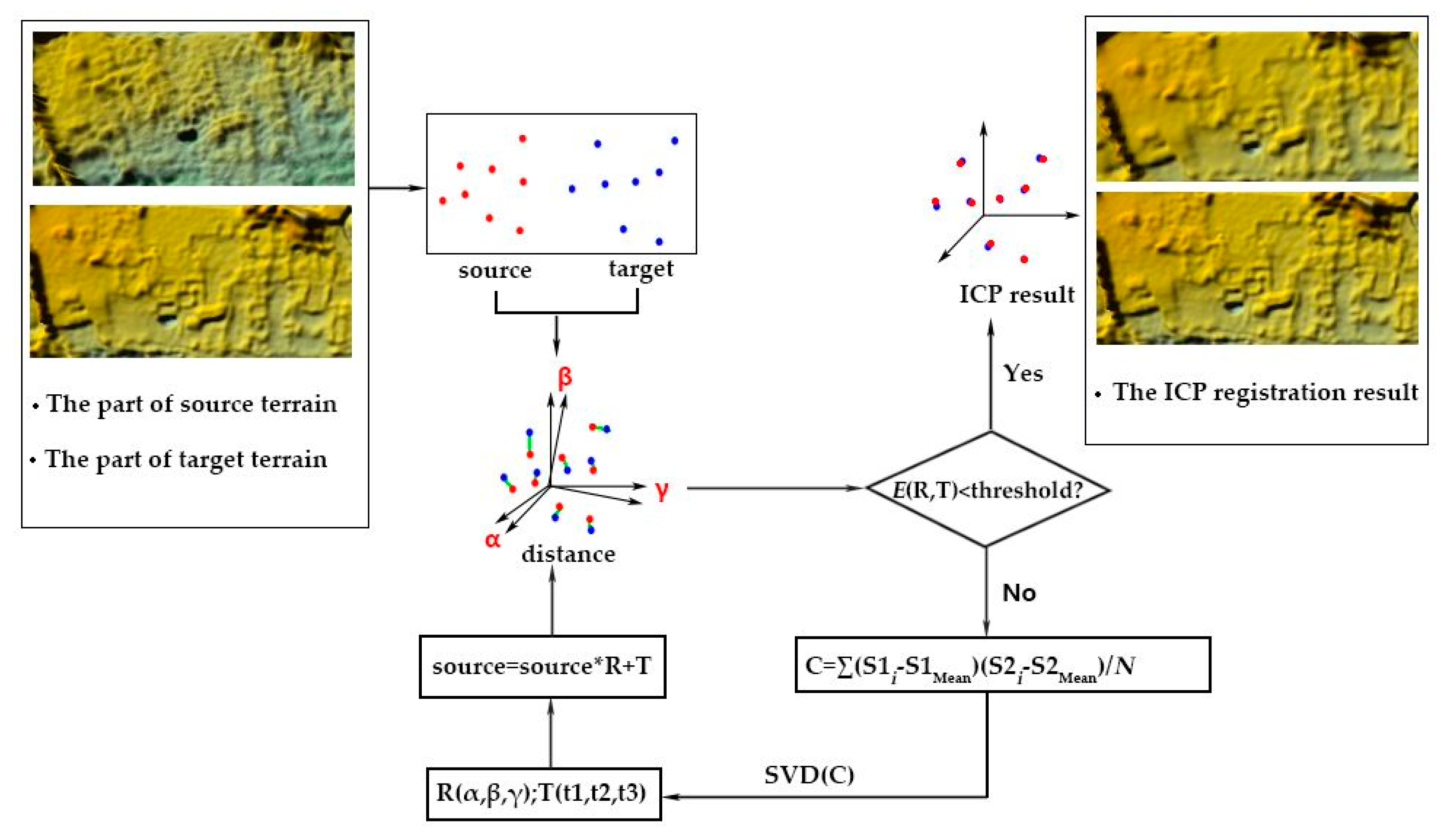
Ideally, the terrain variation in the two periods can be calculated and analysed on the basis of the aforementioned procedure as long as both point sets are correctly georeferenced. However, the deviation in the horizontal and vertical coordinate frames between the two point sets occurs because of inaccurate positioning and variation in the vertical direction [27,29,30]. If not addressed properly, the deviation could seriously affect the results of topographical change analysis. To address the problem, we applied the ICP algorithm to transfer the two point sets acquired by different sensors into the same common coordinate system. Figure 1 shows the basic flow of the ICP algorithm.
A given surface can be described as a point set. The two point sets describing the same surface collected by different sensors could be represented in three dimensions as and , respectively. Let S1 be the source point set, and S2 be the target point set; S1 is not necessarily equal to S2. No pre-established correspondence exists between the point sets. One of the point sets generally undergoes certain transformations such as translation and rotation to match with the other point set. The equation can be expressed as
where R is a 3D rotation matrix and the T is a translation vector.
The ICP algorithm attempts to find the best transformation relationship between point sets that aligns the source point set with the target point set. For this purpose, the following cost function E(R, T) is used:
To derive the 3D rotation matrix R and translation vector T, the covariance matrix C is decomposed by using the singular value decomposition:
where , are the mean values of the point sets and , respectively.
An iterative search is conducted to derive the pre-established correspondence between the source point set and the target point set. At each iteration, a correspondence is established, and the transformation that minimises the mean square metric is computed. The data points are transformed using the computed transformation, and the process is repeated whilst reducing the given cost function E(R, T) until it is less than the given threshold, or until a maximum number of iterations is reached.
2.3. Detection of Terrain Variations
With the ICP algorithm, two different temporal point sets can be registered in the same coordinate system. Then, the dynamic information of the terrain can be calculated on the basis of the SD of dH (σdH) in the region. In theory, σdH can be obtained by [Equation (2)], however, accurately modelling σdH for bathymetric data, whose uncertainty knowledge is rarely available, is difficult because of the numerous factors during MBES measurement that may complicate the noise model in unfavourable underwater conditions [31]. Therefore, we focused on the local statistical distribution of dH and estimated the σdH value from a phenomenon point of view. Specifically, the whole study area was divided into several subareas by using a circular sliding window, with each point in the point set as the centre point with a radius of 5 m. Then, the SD of dH was calculated locally in the window.
Two factors are considered in choosing the size of the sliding window. First, given a small window, the resulting variance estimate would show a strong statistical fluctuation due to the limited size of the samples in the window. Second, a large window would weaken the representation of the variance estimate. Thus, a trade-off exists in choosing the size of the sliding window. In our study, the radius of the sliding window was set as 5 m. In each circular window, the SD of local dH was computed as
where is the SD of the k-th window; is the dH value of the i-th point in the k-th window; and dHmean is the mean value in the window given as
Generally, the aforementioned statistics are efficient for Gaussian-distributed variables. However, for our datasets, the potential existence of topographical changes and outliers in measurements are not consistent with such a Gaussian assumption. If not addressed properly, then the computed variance will be seriously biased by the outliers [32,33]. Hence, the variance of depth difference in the local window in the current work was estimated using the robust estimation procedure. Specifically, the robust counterparts of the mean and the SD statistics were calculated. The empirical formula for the SD of the local region is represented as
where is the median value in the k-th window.
Given the variance estimate, if the points in the window have not undergone any change, then the distribution of dH values will conform to a standard normal distribution. If the absolute value of a depth difference value exceeds a certain threshold (3σ in this study), then the point will be considered having undergone a significant change. Thus, by traversing all the depth difference values based on Equations (12)–(14), the points can be flagged [24].
where Sk is the circular region with a radius of 5 m. is the confidence level and is the corresponding value when the confidence level is equal to /2.
3. Experiment and Results
3.1. Study Area and Data Collection
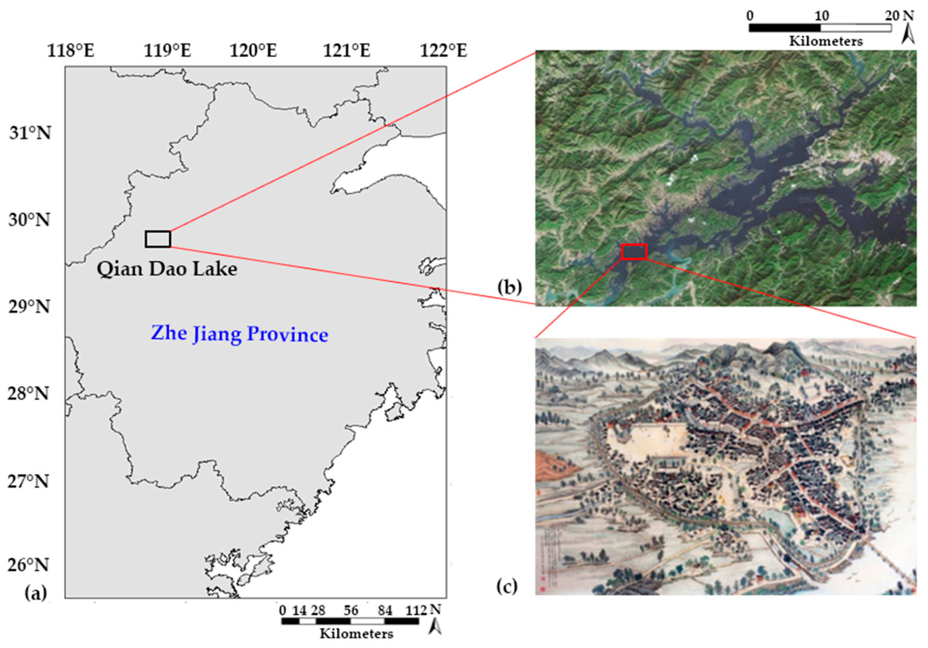
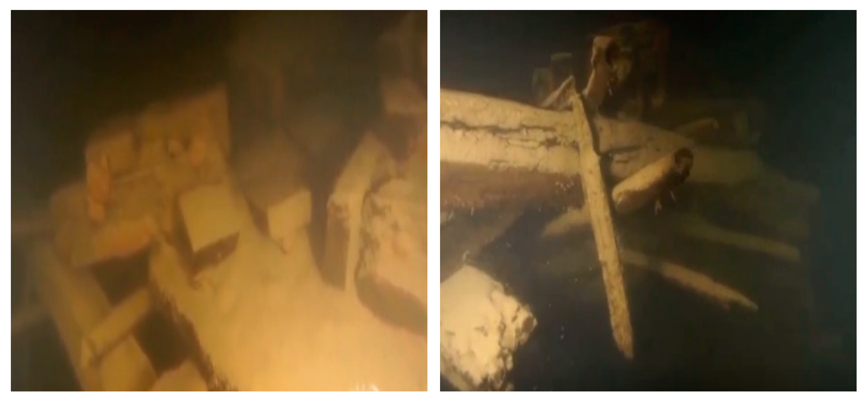
The study area is the ancient town of Chunan, which is submerged in Qiandao Lake. Located in Hangzhou City, China, Qiandao Lake is a vast inland lake with an area of approximately 567.4 km² and an average depth of about 34 m (Figure 2). In September 1959, the town of Lion City in Chunan County, with a long history of over a thousand years, was submerged underwater due to the building of the Xin’anjiang Hydroelectric Plant. Significant underwater terrain variation can be expected due to the damage of the ancient buildings, as shown in Figure 3. Hence, the MBES should be employed for repeated measurements to monitor and evaluate the temporal topographical variations of the town.
Two datasets collected at different times were used for the analysis in this study. The first dataset was collected in 2002 with an EM3000 system. In the survey, the swath angle was set to 100°, and the beam number and depth resolution were 127 and 1 cm, respectively. The average point density was equal to 1.2 points per m2, and the average value of the depth measurements was 31.54 m. The second dataset was collected in 2015 using the SONIC2024 system. In the survey, the swath angle was about 120°, and the beam number and depth resolution were 256 and 1.25 cm, respectively. To ensure that the whole terrain was surveyed, the interval distance between survey lines was set corresponding to the depth to provide overlap in the adjacent lines. The average point resolution was 1.5 m, and the average depth was 30.75 m.
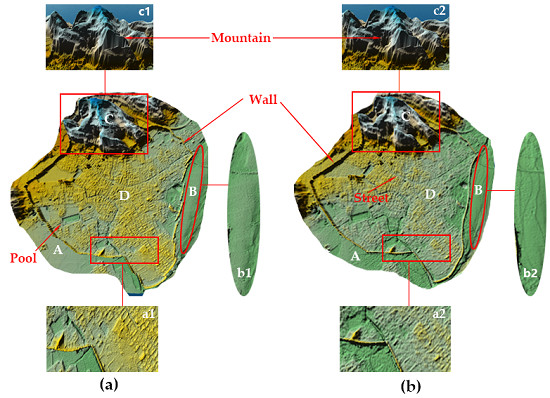
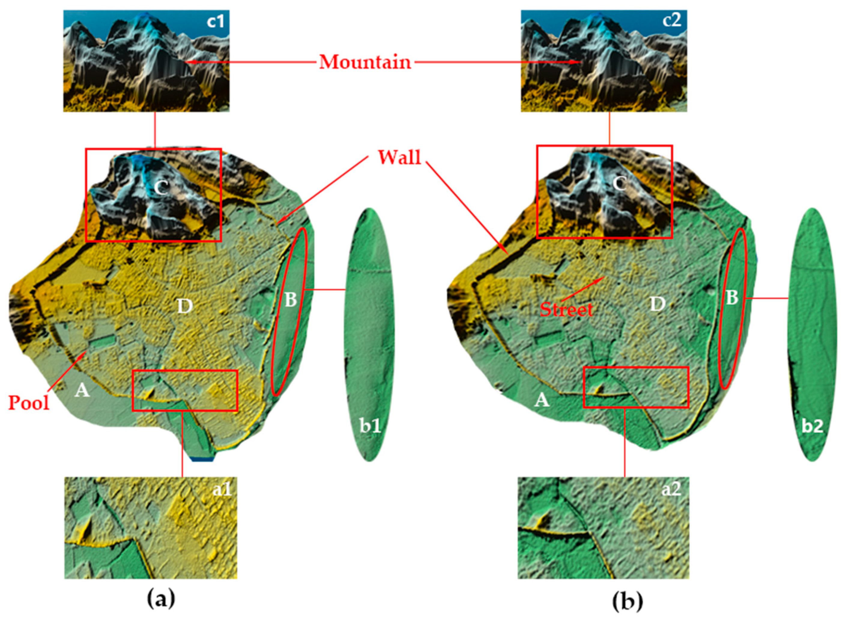
Prior to analysis, the bathymetric data were processed using the commercial software CARIS HIPS/SISP 9.1. The specific procedure was as follows: (1) swath edit (mainly removing the noise points and outliers manually); (2) sound velocity correction; (3) tidal correction; (4) data fusion; (5) calibration of the installation parameters; and (6) data refusion and exporting of bathymetric data. Subsequently, the bathymetric data were converted into the XYZ format. Gridded DEMs with a resolution of 1 m were generated by interpolating the point cloud with the Golden Surfer 16. 0 software, as shown in Figure 4. Visual judgment revealed that the main features around the town including the walls, roads, pond, and private houses were well preserved and visible. The current status of the Lion City is in full compliance with the historical records, indicating an area of about 0.432 km² and wall length of approximately 2.57 km. For easy visualisation and analysis, the town and surrounding areas were divided into four regions: A, B, C, and D. Regions A and B were set as the marginal zones of the outer wall of the town with a relatively flat terrain. Region C was characterised as being covered by mountains with great topographic relief. Region D represented the ancient town with visible outlines of the streets and walls.
3.2. Registration of Point Sets
The systematic residuals and calibration residuals between two datasets collected by different types of MBES may present differences. Hence, the coordinate frames of the two datasets will be inevitably inconsistent. Therefore, the ICP algorithm was applied in this work to reduce the coordinate deviation. Unless the residual value reaches the threshold, the iteration in the ICP algorithm is terminated to ensure optimal registration.
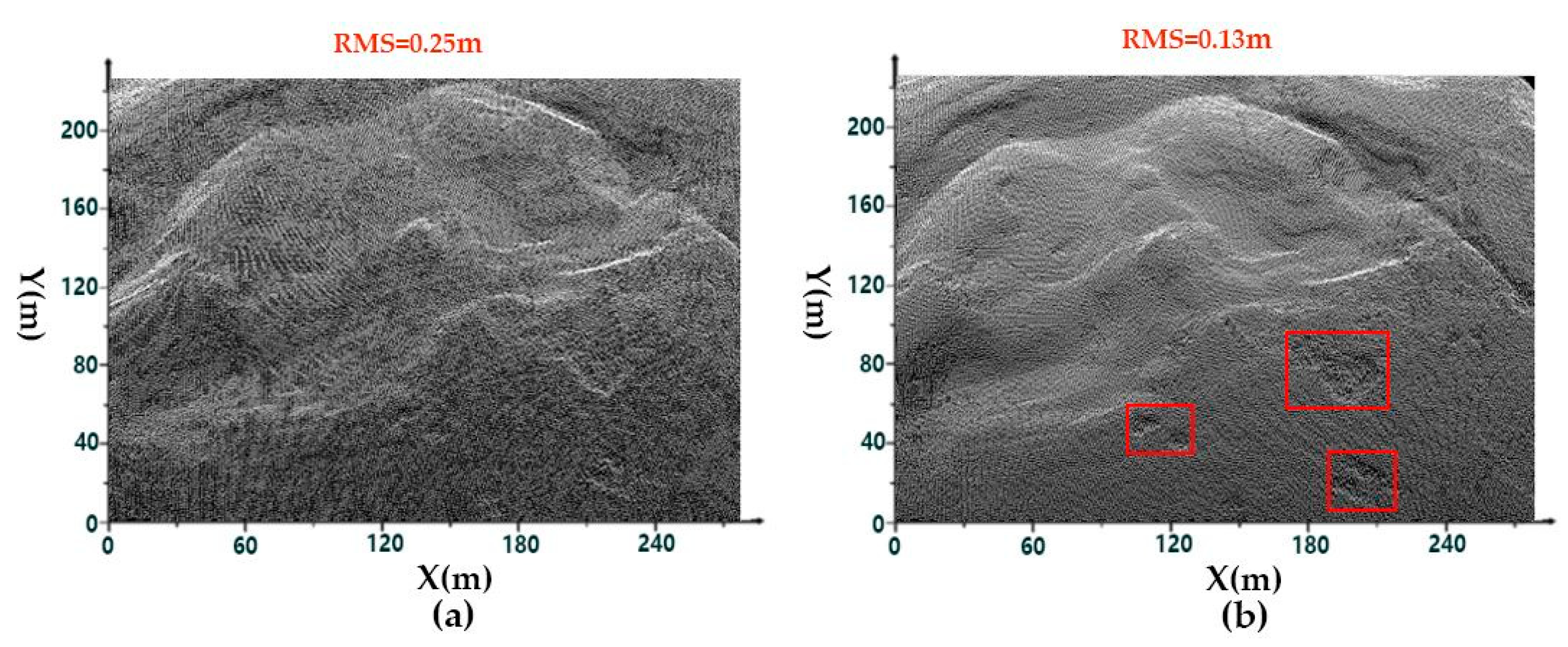
As shown in Figure 5, region C, which was covered by mountains with obvious topographical relief, was extracted to highlight the area with a significant contrast effect from the ICP algorithm. Figure 5 shows that relative to the right image in Figure 5b, the morphological features in the left image in Figure 5a are blurry. Hence, detecting topographical changes was challenging. After being registered by the ICP algorithm, the root mean square (RMS) of DoD dropped from 0.25 m to 0.13 m. The terrain features are marked by red frames in Figure 5b.
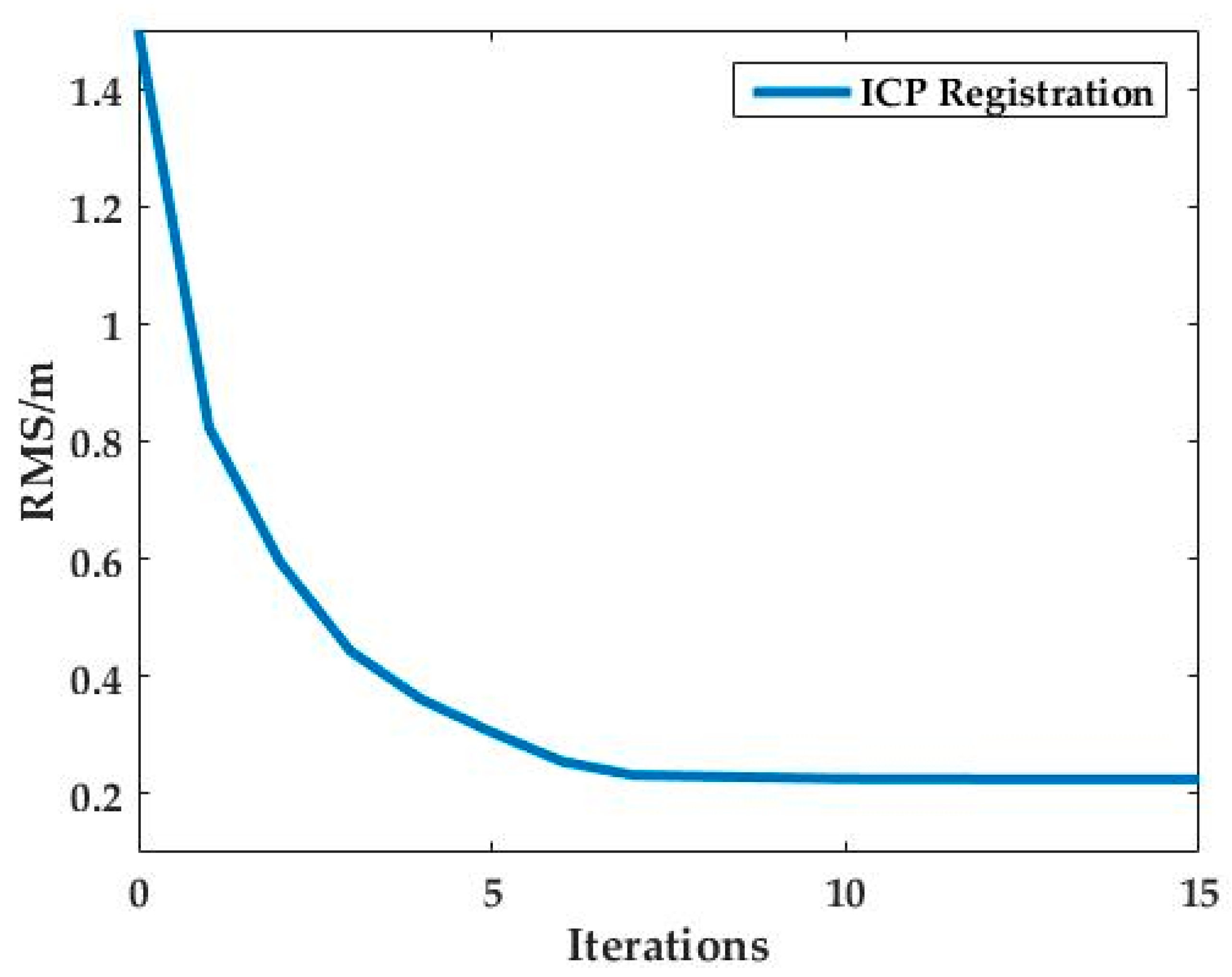
Figure 6 shows the residual variation during the ICP computation process. The residuals around the whole study area dropped from 1.44 m to 0.21 m. By minimising the residuals, the bias between the two datasets in the X and Y direction were identified as 0.01 and 0.16 m, respectively.
3.3. Regional Analysis
With two point sets being registered, six different statistics (Table 1) of DoD in the four regions, (i.e., A, B, C and D, Figure 4) were calculated.
On the global scale, the temporal variation of terrain is relatively small, as indicated by the mean, the mean absolute value (MAV), and the root mean square (RMS) (Table 1), while from a local perspective, there is an evident difference in the bathymetric variation patterns among different local regions. Generally, the MAVs and RMS in regions A and B are greater than those in regions C and D. This indicates that the temporal variation in bathymetry is more evident in regions A and B. Specifically, the mean depth change values were −0.01 m for region A, which presented an erosion feature; and 0.04 m in region B, which indicated a deposition pattern. As for regions C and D, the mean depth change values were both negligible, which indicates insignificant temporal bathymetry changes around these regions.
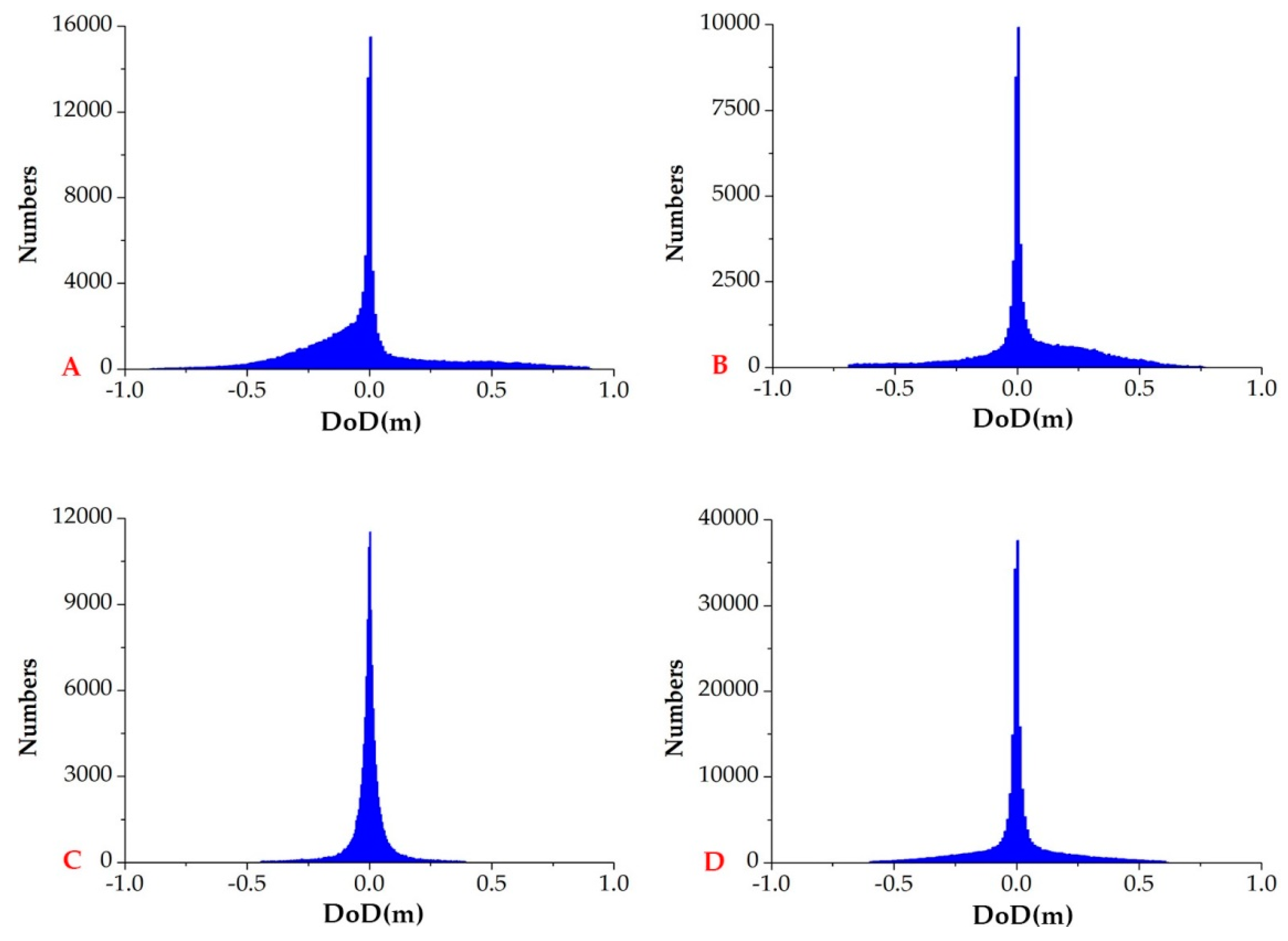
Similar patterns were also revealed by the histograms of the DoD values. As shown in Figure 7, evident bathymetry variations are presented in regions A and B. Specifically, the heavy tail in the left hand side of the histogram indicates a general erosion pattern in region A. On the contrary, region B is shown to have a significant deposition pattern, while for regions C and D, the histograms were generally symmetrical, and are similar to the standard normal distribution.
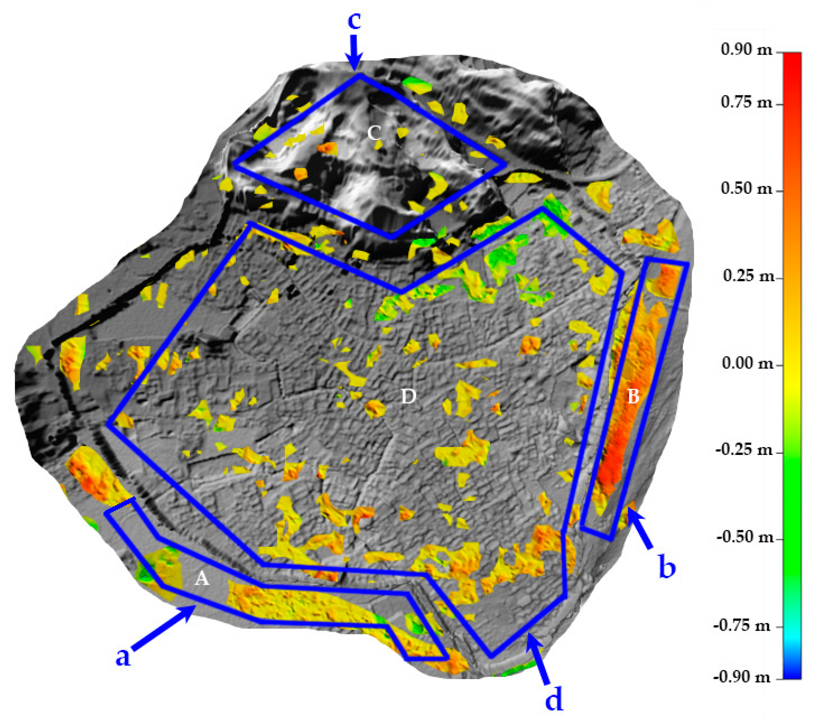
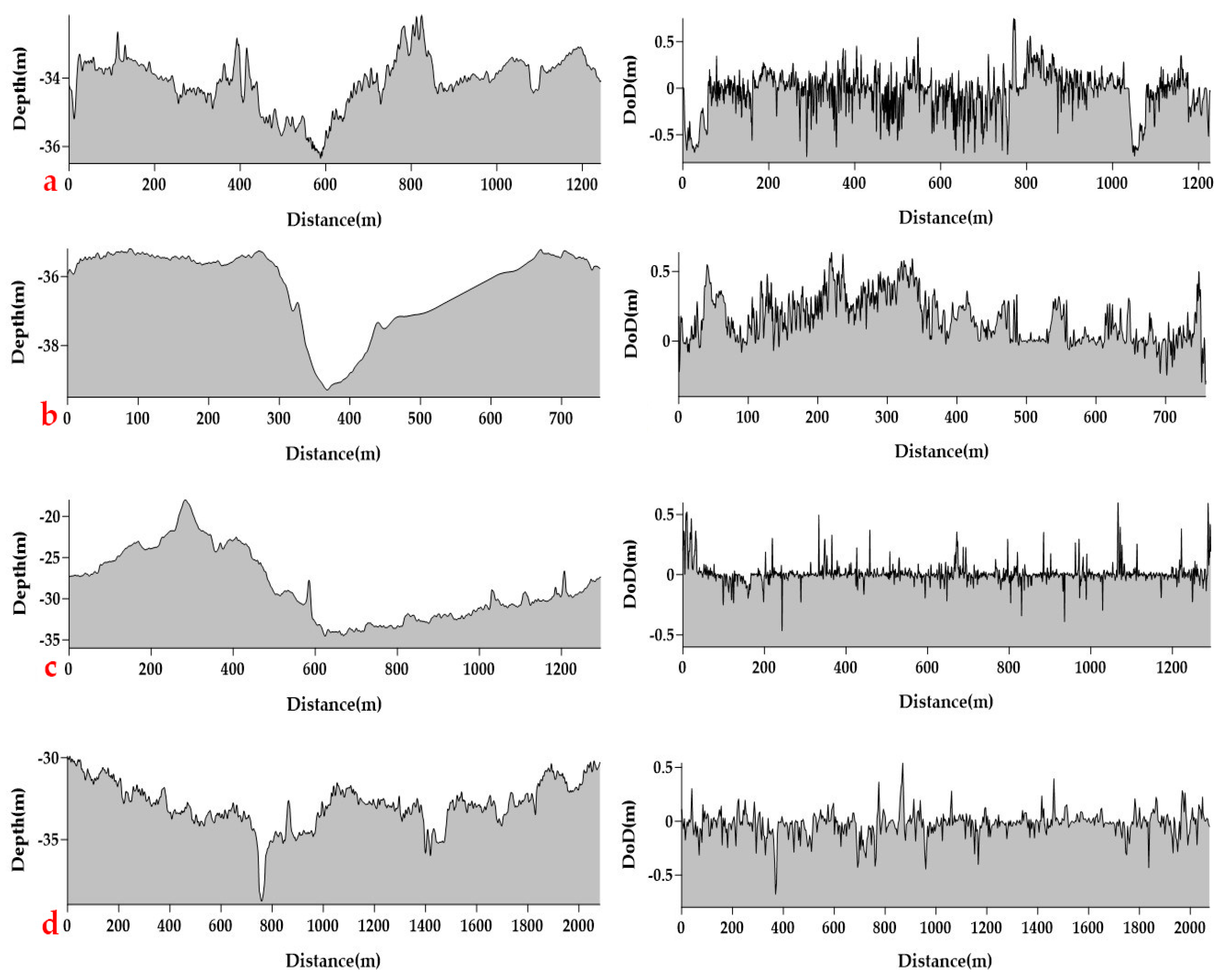
On the basis of robust estimation, the specific areas experiencing topographical changes were detected. First, the variances of the DoD in the local sliding window were calculated. Second, the confidence level of the DoD was set to 99.7% to identify the areas with significant bathymetry variations. Figure 8 shows the spatial distribution of the identified topographical variations. In region A, a mix of erosion and light deposition was observed. The deposition was predominant in region B, and an increasing tendency was revealed along the wall. On the contrary, few topographical changes were observed in regions C and D. To better illustrate the bathymetry variation pattern, four representative profiles are shown for their DoD and bathymetry information (Figure 9).
4. Discussion
4.1. Various Threats to the Ancient Town
The Lion City is an ancient town with a history of over a thousand years. It is a part of a large-scale ancient community that includes several other ancient towns (the Crane City, the Weiping Town, the Port Town, and the Tea Plantation Town). All of the ancient towns have been submerged in the Xin’anjiang Reservoir for more than 60 years. Generally, the terrain in the reservoir environment is often subjected to significant bathymetry variation due to the influence of underwater currents [34,35]. Moreover, human activities in Qiandao Lake such as dredging and fishing activities can also cause an evident variation of underwater topography. All of these factors pose a significant threat to the conservation of the underwater ancient towns. For instance, the walls and architectures built with vulnerable bricks and glued with lime and other materials may collapse due to the pressure generated by the near-bottom current. Thus, monitoring the temporal topography variation of the ancient towns based on repeated surveys can provide critical information for the heritage conservation management.
4.2. Validation of Analysis
When comparing two repeated bathymetric datasets, the differences in depth resulting from measurement errors can be approximated by a normal distribution. In contrast, the morphological changes of underwater targets can be regarded as outliers. Thus, the temporal changes of the bathymetry around the ancient town can be identified by using hypothesis testing based on DoD values. The robust estimation revealed slight terrain variations in the study area on the global scale. The mean and MAV of DoD value were 0 and 0.10 m, respectively. This finding is consistent with the conclusion of Zhang that the geological environment of Qiandao Lake is stable and that the corresponding annual crust deformation is around 1.1 cm [36]. On the contrary, large terrain variations were identified in some local regions. The spatial distribution of the DoD (Figure 8) indicates that the locations with evident terrain variations are located mainly outside the town wall in regions A and B. This pattern is presumably caused by the influence of the interaction between the underwater current and the wall. For sites located inside the wall, the cause of the significant terrain variation is probably the architectural deformation. In conclusion, all of these findings suggest that the ancient town located underwater is subjected to significant stress due to the influence of hydrological and chemical factors.
4.3. Monitoring Suggestions for Ancient Town
The proposed method provides a practical way to understand the characterisations of the topographical changes in the study area. Combining the data collected by the MBES with multitemporal analysis is a tractable, effective, and labour-saving method to determine the dynamics of the town. However, the uncertainty in MBES datasets may prevent the detection of actual surface changes as these datasets are based merely on dH values containing all the information on topographical changes [37]. However, the current methods of estimating topographical changes based on MBES data including determining the difference between two MBES datasets under a stable feature assumption [38,39] or subtracting crest lines and trough lines [40,41], are unable to completely remove the disturbance of outliers; hence, the assessment of terrain variations remains challenging. In addition, these methods do not consider the uncertainty in their calculation. Therefore, we suggest that before using the robust estimation, the impacts of outliers should be mitigated as much as possible. In future research, data from various sources should be used to enhance the accurate characterisation of the dynamics of ancient towns.
4.4. Conservation Suggestion of Ancient Towns
The ancient town of Chunan has been submerged in Qiandao Lake for more than 60 years. Recently, the value of this ancient town in culture and tourism has been recognised by the local government. In 2011, Lion City was listed as a heritage conservation unit of Zhejiang Province. However, shipping, fishing, and dredging are still prevalent in Qiandao Lake. Moreover, the frequent variations in water levels due to the storage and discharge of the Xian Reservoir can generate large underwater currents. Although Section 3 showed that the overall depth variation was insignificant, a significant deformation pattern was identified for the local area inside and outside the town wall. Thus, protecting the underwater ancient town requires a strict and targeted policy to balance economic development and heritage conservation. In this context, repeated MBES surveys can effectively collect information about the state of the underwater architecture. Thus, appropriate policy making and management will require an increased frequency of MBES bathymetry surveys around the area.
5. Conclusions
Repeated MBES surveys provide valuable information about the topography variation of the ancient town of Chunan. In this study, we combined the ICP algorithm and the robust estimation method to characterise the time-varying topographical features of the ancient town between 2002 and 2015. The computation result showed an insignificant global terrain change pattern. In contrast, large topographical changes were identified in a number of local areas. The experimental results verified the feasibility of applying the MBES to effectively quantify the time-varying topographical changes of the underwater ancient town. Furthermore, the result is of reference value for formulating government policies about the ancient town. In future study, the characterisation of the dynamics of the ancient town can benefit greatly from long-term MBES surveys with an increased frequency.
Author Contributions
Conceptualization, F.Y. and K.Z.; Methodology K.Z. and F.X.; Software, F.X.; Validation, F.Y. and K.Z.; Formal analysis, K.Z., X.B., and F.X.; Resources, H.H.; Writing—original draft preparation, F.X.; Writing—review & editing, K.Z., X.B., M.A., and F.X.; Visualization, K.Z. and F.X.; Supervision, K.Z. and X.B. Funding acquisition, F.Y. and K.Z. All authors have read and agree to the published version of the manuscript.
Funding
This study was jointly funded by the National Natural Science Foundation of China (Nos. 41930535 and 41830540), the National Key R&D Program of China (Nos. 2018YFF0212203, 2017YFC1405006, 2018YFC1405900, in part by the China Postdoctoral Science Foundation funded project under Grant 19202, and 2016YFC1401210), and the SDUST Research Fund (No. 2019TDJH103).
Acknowledgments
We appreciate the MBES data of the first period provided by Yongting Wu from the First Institute of Oceanography, Ministry of Natural Resources of the People’s Republic of China.
Conflicts of Interest
The authors declare no conflict of interest.
References
- Bailey, G.N.; Flemming, N.C. Archaeology of the continental shelf: Marine resources, submerged landscapes and underwater archaeology. Quat. Sci. Rev. 2008, 27, 2153–2165. [Google Scholar] [CrossRef] [Green Version]
- Halligan, J.J.; Waters, M.R.; Angelina, P.; Owens, I.J.; Feinberg, J.M.; Bourne, M.D.; Fenerty, B.; Winsborough, B.; Carlson, D.; Fisher, D.C.; et al. Pre-Clovis occupation 14, 550 years ago at the Page-Ladson site, Florida, and the peopling of the Americas. Sci. Adv. 2016, 2, e1600375. [Google Scholar] [CrossRef] [PubMed] [Green Version]
- Eriksson, N.; Rönnby, J. Mars (1564): The initial archaeological investigations of a great 16th-century Swedish warship. Int. J. Naut. Archaeol. 2017, 46, 92–107. [Google Scholar] [CrossRef] [Green Version]
- Auer, J.; Firth, A. The ‘gresham ship’: An interim report on a 16th-century wreck from princes channel, thames estuary. Post Mediev. Archaeol. 2007, 41, 222–241. [Google Scholar] [CrossRef]
- Ono, R.; Katagiri, C.; Kan, H.; Nagao, M.; Sakagami, N. Discovery of iron grapnel anchors in early modern ryukyu and management of underwater cultural heritage in okinawa, japan. Int. J. Naut. Archaeol. 2016, 45, 77–93. [Google Scholar] [CrossRef]
- McCawley, J.C.; Pearson, C. Conservation of Marine Archaeological Objects. Stud. Conserv. 1991, 36, 121. [Google Scholar] [CrossRef]
- Anderson, D.G.; Bissett, T.G.; Yerka, S.J.; Wells, J.J.; Kansa, E.C.; Kansa, S.W.; Myers, K.N.; DeMuth, R.C.; White, D.A. Sea-level rise and archaeological site destruction: An example from the southeastern United States using DINAA (Digital Index of North American Archaeology). PLOS ONE 2017, 12, e0188142. [Google Scholar] [CrossRef] [Green Version]
- Stevenson, P. A titanic struggle: One possible resolution of the conflict between preservation for the public good and private law property rights. Art Antiq. Law Leic. 2011, 16, 53–66. [Google Scholar]
- Petriaggi, R. The role of the italian central institute of restoration in the field of underwater archaeology. Int. J. Naut. Archaeol. 2002, 31, 74–82. [Google Scholar] [CrossRef]
- Gregory, J.D. Formation Processes in Underwater Archaeology: A Study of Chemical and Biological Deterioration. Ph.D. Thesis, University of Leicester, Leicester, UK, 1996. [Google Scholar]
- Crisci, G.M.; Russa, M.F.L.; Macchione, M.; Malagodi, M.; Palermo, A.M.; Ruffolo, S.A.; La Russa, M.F. Study of archaeological underwater finds: Deterioration and conservation. Appl. Phys. A 2010, 100, 855–863. [Google Scholar] [CrossRef]
- Harmsen, H.; Hollesen, J.; Madsen, C.K.; Albrechtsen, B.; Myrup, M.; Matthiesen, H. A Ticking Clock? Preservation and Management of Greenland’s Archaeological Heritage in the Twenty-First Century. Conserv. Manag. Archaeol. Sites 2018, 20, 175–198. [Google Scholar] [CrossRef]
- Stewart, W.K. Multisensor Visualization for Underwater Archaeology. IEEE Comput. Soc. Press 1991, 11, 13–18. [Google Scholar] [CrossRef]
- Bass, G.F.; Pulak, C.; Collon, D.; Weinstein, J. The Bronze Age Shipwreck at Ulu Burun: 1986 Campaign. Am. J. Archaeol. 1989, 93, 1–29. [Google Scholar] [CrossRef]
- Mccarthy, J.K.; Benjamin, J.; Winton, T.; Van Duivenvoorde, W. The Rise of 3D in Maritime Archaeology. In 3D Recording and Interpretation for Maritime Archaeology; Springer: New York, NY, USA, 2019. [Google Scholar]
- Pacheco-Ruiz, R.; Adams, J.; Pedrotti, F. 4D modelling of low visibility Underwater Archaeological excavations using multi-source photogrammetry in the Bulgarian Black Sea. J. Archaeol. Sci. 2018, 100, 120–129. [Google Scholar] [CrossRef] [Green Version]
- Westley, K.; Mcneary, R. Archaeological Applications of Low-Cost Integrated Sidescan Sonar/Single-Beam Echosounder Systems in Irish Inland Waterways. Archaeol. Prospect. 2016, 24, 37–57. [Google Scholar] [CrossRef] [Green Version]
- Doneus, M.; Doneus, N.; Briese, C.; Pregesbauer, M.; Mandlburger, G.; Verhoeven, G. Airborne laser bathymetry—Detecting and recording submerged archaeological sites from the air. J. Archaeol. Sci. 2013, 40, 2136–2151. [Google Scholar] [CrossRef]
- Bates, C.R.; Lawrence, M.; Dean, M.; Robertson, P. Geophysical Methods for Wreck-Site Monitoring: The Rapid Archaeological Site Surveying and Evaluation (RASSE) programme. Int. J. Naut. Archaeol. 2010, 40, 404–416. [Google Scholar] [CrossRef]
- Poglajen, S. Acoustic Data in Underwater Archaeology. In Proceedings of the Computer Applications & Quantitative Methods in Archaeology (CAA) 2012 Conference, University of Southampton, Southampton, UK, 26–30 March 2012. [Google Scholar]
- Plets, R.; Quinn, R.; Forsythe, W.; Westley, K.; Bell, T.; Benetti, S.; Robinson, R. Using multi-beam Echo-Sounder Data to Identify Shipwreck Sites: Archaeological assessment of the Joint Irish Bathymetric Survey data. Int. J. Naut. Archaeol. 2011, 40, 87–98. [Google Scholar] [CrossRef]
- Ernstsen, V.B.; Noormets, R.; Winter, C.; Hebbeln, D.; Bartholomä, A.; Flemming, B.W.; Bartholdy, J. Development of subaqueous barchanoid-shaped dunes due to lateral grain size variability in a tidal inlet channel of the Danish Wadden Sea. J. Geophys. Res. Space Phys. 2005, 110. [Google Scholar] [CrossRef]
- Tassetti, A.N.; Malaspina, S.; Fabi, G. Using a multi-beam Echosounder to Monitor AN Artificial Reef. ISPRS. Int. Arch. Photogramm. Remote Sens. Spat. Inf. Sci. 2015, XL-5/W5, 207–213. [Google Scholar] [CrossRef] [Green Version]
- Clarke, J.E.H.; Mayer, L.A.; Wells, D.E. Shallow-water imaging multi-beam sonars: A new tool for investigating seafloor processes in the coastal zone and on the continental shelf. Mar. Geophys. Res. 1996, 18, 607–629. [Google Scholar] [CrossRef]
- Bu, X.; Yang, F.; Ma, Y.; Wu, D.; Zhang, K.; Xu, F. Simplified calibration method for multibeam footprint displacements due to non-concentric arrays. Ocean Eng. 2020, 197, 106862. [Google Scholar] [CrossRef]
- Jian-Lin, M.A.; Jing, J.; Xiang-Hua, L. The Construction of Seafloor Digital Terrain Model Based on multi-beam Soundings. Hydrogr. Surv. Charting 2005, 25, 15–17. [Google Scholar]
- Schimel, A.C.G.; Ierodiaconou, D.; Hulands, L.; Kennedy, D.M. Accounting for uncertainty in volumes of seabed change measured with repeat multi-beam sonar surveys. Cont. Shelf Res. 2015, 111, 52–68. [Google Scholar] [CrossRef]
- Zhu, W.Q.; Wei, J.J.; Li, M.W.; Yin, D.Y. Random error model of multi-beam echo-sounding sonar. J. Mar. Technol. 1986, 2, 98–105. [Google Scholar]
- Guériot, D.; Chèdru, J.; Daniel, S.; Maillard, E. The patch test: A comprehensive calibration tool for multi-beam echosounders. In Proceedings of the OCEANS 2000 MTS/IEEE Conference and Exhibition, Providence, RI, USA, 11–14 September 2000. [Google Scholar]
- Smith, D.P.; Kvitek, R.; Iampietro, P.J.; Wong, K. Twenty-nine months of geomorphic change in upper Monterey Canyon (2002–2005). Mar. Geol. 2007, 236, 79–94. [Google Scholar] [CrossRef]
- Brothers, L.L.; Kelley, J.T.; Belknap, D.F.; Barnhardt, W.A.; Andrews, B.D.; Maynard, M.L. More than a century of bathymetric observations and present-day shallow sediment characterization in Belfast Bay, Maine, USA: Implications for pockmark field longevity. Geophys. Mar. Lett. 2011, 31, 237–248. [Google Scholar] [CrossRef] [Green Version]
- Zhang, K.; Yang, F.L.; Zhao, C.; Feng, C. Using robust correlation matching to estimate sand-wave migration in Monterey Submarine Canyon, California. Mar. Geol. 2016, 376, 102–108. [Google Scholar] [CrossRef]
- Nygren, I.; Jansson, M. Terrain navigation for underwater vehicles using the correlator method. IEEE J. Ocean. Eng. 2004, 29, 906–915. [Google Scholar] [CrossRef]
- Blas, L.; Valero, G.; Navas, A.; Javier, M.; Walling, D. Sediment sources and siltation in mountain reservoirs: A case study from the central spanish pyrenees. Geomorphology 1999, 28, 23–41. [Google Scholar]
- Abraham, J. Spatial distribution of major and trace elements in shallow reservoir sediments: An example from lake waco, texas. Environ. Geol. 1998, 36, 349–363. [Google Scholar] [CrossRef]
- Zhang, W. Crustal Deformation Monitoring Based on D-InSAR Technology in Hangzhou Area and Study on Deformation Mechanism. Ph.D. Thesis, Zhejiang University, Zhejiang, China, 2008. [Google Scholar]
- Clarke, J.E.H. Dynamic motion residuals in swath sonar data: Ironing out the creases. Int. Hydrogr. Rev. 2003, 4, 6–23. [Google Scholar]
- Dorst, L.L.; Roos, P.C.; Hulscher, S.; Lindenbergh, R.C. The estimation of sea floor dynamics from bathymetric surveys of a sand wave area. J. Appl. Geodesy 2009, 3, 97–120. [Google Scholar] [CrossRef]
- Dorst, L.L.; Roos, P.C.; Hulscher, S. Spatial differences in sand wave dynamics between the Amsterdam and the Rotterdam region in the Southern North Sea. Cont. Shelf Res. 2011, 31, 1096–1105. [Google Scholar] [CrossRef]
- Cherlet, J.; Besio, G.; Blondeaux, P.; Van Lancker, V.; Verfaillie, E.; Vittori, G. Modeling sand wave characteristics on the Belgian Continental Shelf and in the Calais-Dover Strait. J. Geophys. Res. 2007, 112. [Google Scholar] [CrossRef] [Green Version]
- Van Dijk, T.A.; Kleinhans, M.G. Processes controlling the dynamics of compound sandwaves in the North Sea, Netherlands. J. Geophys. Res. 2005, 110. [Google Scholar] [CrossRef]
Figure 1.
Schematic of the principle and workflow of the iterative closest point (ICP) algorithm.

Figure 2.
(a) Location of Qiandao Lake. (b) Satellite image of Qiandao Lake. (c) Picture painted to restore the original appearance of the town.
Figure 2.
(a) Location of Qiandao Lake. (b) Satellite image of Qiandao Lake. (c) Picture painted to restore the original appearance of the town.

Figure 3.
Damage of the underwater ancient town in Qiandao Lake.

Figure 4.
Shaded relief images generated with bathymetric data acquired by MBES in 2002 (a) and 2015 (b).
Figure 4.
Shaded relief images generated with bathymetric data acquired by MBES in 2002 (a) and 2015 (b).

Figure 5.
Validation verification of the ICP algorithm. (a,b) Terrain feature comparison of overlapped point clouds in region C before and after registration, respectively. The areas in red rectangles are used to show the significant terrain features.
Figure 5.
Validation verification of the ICP algorithm. (a,b) Terrain feature comparison of overlapped point clouds in region C before and after registration, respectively. The areas in red rectangles are used to show the significant terrain features.

Figure 6.
Residual variation in the ICP computation process.

Figure 7.
Histogram of DEM of Difference (DoD) values for four regions of the study area.

Figure 8.
Spatial distribution of topographical changes in the ancient town.

Figure 9.
Comparison of the depth and DoD values for four representative profiles of the four regions.
Figure 9.
Comparison of the depth and DoD values for four representative profiles of the four regions.


Table 1.
Statistics of the comparison of DoD values for four regions of the town.
| Region | Minimum (m) | Maximum (m) | Mean (m) | MAV (m) | RMS (m) |
|---|---|---|---|---|---|
| Global | −0.89 | 0.88 | 0 | 0.12 | 0.21 |
| A | −0.89 | 0.88 | −0.01 | 0.18 | 0.27 |
| B | −0.76 | 0.69 | 0.04 | 0.16 | 0.25 |
| C | −0.41 | 0.39 | 0 | 0.06 | 0.13 |
| D | −0.61 | 0.60 | 0 | 0.10 | 0.19 |
© 2020 by the authors. Licensee MDPI, Basel, Switzerland. This article is an open access article distributed under the terms and conditions of the Creative Commons Attribution (CC BY) license (http://creativecommons.org/licenses/by/4.0/).
Share and Cite
MDPI and ACS Style
Yang, F.; Xu, F.; Zhang, K.; Bu, X.; Hu, H.; Anokye, M. Characterisation of Terrain Variations of an Underwater Ancient Town in Qiandao Lake. Remote Sens. 2020, 12, 268. https://0-doi-org.brum.beds.ac.uk/10.3390/rs12020268
AMA Style
Yang F, Xu F, Zhang K, Bu X, Hu H, Anokye M. Characterisation of Terrain Variations of an Underwater Ancient Town in Qiandao Lake. Remote Sensing. 2020; 12(2):268. https://0-doi-org.brum.beds.ac.uk/10.3390/rs12020268
Chicago/Turabian StyleYang, Fanlin, Fangzheng Xu, Kai Zhang, Xianhai Bu, Hao Hu, and Michael Anokye. 2020. "Characterisation of Terrain Variations of an Underwater Ancient Town in Qiandao Lake" Remote Sensing 12, no. 2: 268. https://0-doi-org.brum.beds.ac.uk/10.3390/rs12020268
Note that from the first issue of 2016, this journal uses article numbers instead of page numbers. See further details here.