Article

Probabilistic Mapping and Spatial Pattern Analysis of Grazing Lawns in Southern African Savannahs Using WorldView-3 Imagery and Machine Learning Techniques

1
Department of Geography and Geology, Edge Hill University, St. Helens Road, Ormskirk L39 4QP, UK
2
Land Use Group, UK Centre for Ecology and Hydrology, Library Ave, Bailrigg, Lancaster LA1 4AP, UK
3
Department of Biology, Edge Hill University, St. Helens Road, Ormskirk L39 4QP, UK
4
Scientific Services, Kruger National Park, Private Bag X402, Skukuza 1350, South Africa
5
Centre for African Ecology, School of Animal, Plant and Environmental Sciences, University of the Witwatersrand, Private Bag 3, Johannesburg 2050, South Africa
*
Author to whom correspondence should be addressed.
Remote Sens. 2020, 12(20), 3357; https://0-doi-org.brum.beds.ac.uk/10.3390/rs12203357
Submission received: 22 September 2020 / Revised: 9 October 2020 / Accepted: 11 October 2020 / Published: 15 October 2020
(This article belongs to the Special Issue Satellite Image Processing and Applications)

Abstract

:
Savannah grazing lawns are a key food resource for large herbivores such as blue wildebeest (Connochaetes taurinus), hippopotamus (Hippopotamus amphibius) and white rhino (Ceratotherium simum), and impact herbivore densities, movement and recruitment rates. They also exert a strong influence on fire behaviour including frequency, intensity and spread. Thus, variation in grazing lawn cover can have a profound impact on broader savannah ecosystem dynamics. However, knowledge of their present cover and distribution is limited. Importantly, we lack a robust, broad-scale approach for detecting and monitoring grazing lawns, which is critical to enhancing understanding of the ecology of these vital grassland systems. We selected two sites in the Lower Sabie and Satara regions of Kruger National Park, South Africa with mesic and semiarid conditions, respectively. Using spectral and texture features derived from WorldView-3 imagery, we (i) parameterised and assessed the quality of Random Forest (RF), Support Vector Machines (SVM), Classification and Regression Trees (CART) and Multilayer Perceptron (MLP) models for general discrimination of plant functional types (PFTs) within a sub-area of the Lower Sabie landscape, and (ii) compared model performance for probabilistic mapping of grazing lawns in the broader Lower Sabie and Satara landscapes. Further, we used spatial metrics to analyse spatial patterns in grazing lawn distribution in both landscapes along a gradient of distance from waterbodies. All machine learning models achieved high F-scores (F1) and overall accuracy (OA) scores in general savannah PFTs classification, with RF (F1 = 95.73 ± 0.004 % , OA = 94.16 ± 0.004 % ), SVM (F1 = 95.64 ± 0.002 % , OA = 94.02 ± 0.002 % ) and MLP (F1 = 95.71 ± 0.003 % , OA = 94.27 ± 0.003 % ) forming a cluster of the better performing models and marginally outperforming CART (F1 = 92.74 ± 0.006 % , OA = 90.93 ± 0.003 % ). Grazing lawn detection accuracy followed a similar trend within the Lower Sabie landscape, with RF, SVM, MLP and CART achieving F-scores of 0.89, 0.93, 0.94 and 0.81, respectively. Transferring models to the Satara landscape however resulted in relatively lower but high grazing lawn detection accuracies across models (RF = 0.87, SVM = 0.88, MLP = 0.85 and CART = 0.75). Results from spatial pattern analysis revealed a relatively higher proportion of grazing lawn cover under semiarid savannah conditions (Satara) compared to the mesic savannah landscape (Lower Sabie). Additionally, the results show strong negative correlation between grazing lawn spatial structure (fractional cover, patch size and connectivity) and distance from waterbodies, with larger and contiguous grazing lawn patches occurring in close proximity to waterbodies in both landscapes. The proposed machine learning approach provides a novel and robust workflow for accurate and consistent landscape-scale monitoring of grazing lawns, while our findings and research outputs provide timely information critical for understanding habitat heterogeneity in southern African savannahs.

1. Introduction

Savannah ecosystems inherently exhibit a considerable degree of variability in structural and physical attributes across their range of occurrence [1]. In Southern Africa, they feature the coexistence of grasses and an overstorey layer of trees with varying gradients of dominance and spatial formations [2]. Within the grassy layer, plant forms are typified structurally by tall bunch grasses and short grass grazing lawns [3], which form a significant component of the heterogeneity in Southern African savannah grasslands [4].
The relative proportions and distribution of grazing lawns and tall bunch grass resources have been directly linked to important ecosystem changes such as fluctuations in herbivore density [5,6] and changing fire regimes [7,8]. For example, the amount of high-quality lawn grasses has been suggested to be the primary natural limiting factor to population size of mega-herbivores such as the white rhinoceros (Ceratotherium simum) and the hippopotamus (Hippopotamus amphibius) [6,7,9]. Additionally, the persistence of grazing lawns creates natural barriers to the spread of fire due to limited above ground fuel biomass that may serve as fuel for the spread of fire [7,10,11]. By contrast, tall bunch grasses keep their moribund growth forms and increase savannah grassland fuel load [7,12]. As such, changes in grazing lawn coverage and distribution could potentially alter the size, frequency and intensity of fire within the landscape [7], with cascading effects for nutrient cycling, plant community composition, habitat structure and biodiversity. Monitoring the occurrence and spatial patterns of grazing lawns is therefore fundamental to understanding the ecology of these vital grassland systems.
Grazing lawns are dynamic and maintained by constant grazing, resulting in a feedback of dense nutrient-rich plant growth that in turn attracts more grazing [10]. Different parts of a landscape may also be predisposed to grazing lawn formation due to localised availability of resources and nutrient hotspots that concentrate grazers. These include areas around water bodies and areas of mineral accumulation (e.g., sodium) [10]. The initiation of a cycle of regular grazing thus appears to be a critical factor for their development and persistence [10,11,12]. Nonetheless, the rates and specific pathways of their development likely depend on factors such as rainfall, fire and soil types [13]. Rainfall has a strong influence on the rate of grass biomass accumulation and the height of tall grass stands [14]. The relative proportion of grazing lawns to high biomass tall grasses is also influenced by dynamics in soil nutrients through their strong influence on grass productivity. Under high rainfall and soil nutrient conditions, increased grazing frequency is required to prevent the invasion of tall-grass competitors [10]. Too infrequent grazing increases the vulnerability of a switch to tall bunch grasses [11]. Fire also consumes grass biomass and has the potential to shift grass community composition and structure within different environmental constraints [15]. Tall bunch grasses with low forage quality dominate fire-driven grassy systems [10,11,12]. Additionally, post-fire regrowth can also attract grazers away from previously established grazing lawns causing them to be invaded by tall bunch grasses [11,12]. The varying spatial and temporal nature of the key interacting factors that drive grazing lawn dynamics urges for a robust landscape-scale approach to better understand their variation over space and time.
Ground-based monitoring of grazing lawn responses to the complex top-down and bottom-up ecological processes is challenging due to the large areas involved. Although ground-based methods can provide more detailed and valuable local insights [16], they are not efficient in capturing regional-scale dynamics—due to the high cost involved—nor do they provide any retrospective information beyond the start of monitoring activities [17]. Remote sensing technology is able to overcome the spatial and temporal limitations, which in combination with ground-based observations, offers valuable tools for accurate, efficient and cost-effective ways for vegetation monitoring [18,19].
Medium resolution satellite imagery such as the Landsat Operational Land Imager (OLI) [20] and Sentinel-2 missions [21] are freely available, with extensive temporal coverage which offers enormous benefits for monitoring vegetation dynamics. Further, recent advances in very high spatial resolution (VHR) satellite imagery such as WorldView-3 presents opportunities to partially overcome limitations in spatial resolution associated with medium resolution imagery, particularly in heterogeneous savannah landscapes [17]. At nadir spatial resolution of 1.24 m [22], the WorldView-3 sensor is able to identify and discriminate between different sized vegetation components such as trees, shrubs and grass patches [17,23]. Additionally, the yellow, red-edge and two near-infrared bands in WorldView-3 imagery provide the capability of reliably detecting photosynthetically active or dying plants and foliar chlorophyll content [24]. As such, various phenological stages of vegetation can be monitored, which is instrumental in dealing with spectral similarity of different savannah vegetation composition [23,25].
In parallel with advances in remote sensing imaging technology, free open source software packages and increased computational power have been developed to facilitate image analysis. The combination of these factors has advanced the use of machine learning algorithms in land cover classification [26]. Among the most popular machine learning classification algorithms are Random Forest (RF) [27], Support Vector Machines (SVM) [28], Decision Trees (DT) [29] and Artificial Neural Network (ANN) [30]. RF, SVM, DT and ANN are nonparametric classifiers and are very efficient in dealing with nonlinear classification problems [26,31], having been proven to be effective in different savannah ecosystems. Camargo et al. [31] demonstrated the utility of RF, SVM, DT and ANN in classifying land cover in the Brazilian Tropical Savannah biome. RF is well known for its flexibility of application on both continuous and categorical datasets, either as a regression or classification algorithm, respectively [26,27]. Symeonakis et al. [32] used RF to classify different land cover types in southern African savannahs and reported a maximum accuracy of 91.1 %. The SVM classifier is popular for its strong ability to generalise in complex nonlinear feature space [28]. SVM was used in seasonal separation of vegetation components in southern African savannahs and gave the highest accuracy score under dry leaf-off conditions compared to k-Nearest Neighbour (k-NN), Maximum Likelihood Classifier (MLC), RF and DT classifiers [23]. The application of DT in an eastern African savannah resulted in an increased mapping accuracy over MLC and SVM, with over 93% overall accuracy [33]. ANN classifiers have been widely used in satellite image classification, due to the capability to adapt and generalise different input data structures [26]. The successful application of ANN has been well demonstrated in different remote sensing contexts, including classification of endangered tree species [34] and dynamic modelling of land cover changes in semi-arid landscapes [35].
Much of the literature on monitoring grazing lawn dynamics in southern African savannahs focuses on localised and controlled experimental studies of responses to the mechanisms that induce their establishment and persistence [4,10,11,12]. There is limited evidence on whether the proposed pathways translate into broad-scale spatial patterns in grazing lawn occurrence. Among the few empirical studies is the work of Archibald et al. [12] who mapped grass structural distribution and found that the extent of grazing lawns was directly related to fire return interval. Though there is substantial information on how different biotic and abiotic factors shape grazing lawns, knowledge of their present cover and distribution, which is critical to understanding habitat heterogeneity, is lacking. More importantly, there is no robust, broad-scale approach for detecting and monitoring grazing lawns to enable comprehensive investigation into their dynamics over space and time, and the implications for broader ecosystem dynamics. Against this backdrop, we seek to develop a robust machine learning framework for mapping grazing lawns in southern African savannahs by (i) parameterising and assessing the quality of Random Forest (RF), Support VectorMachines (SVM), Multilayer Perceptron (MLP) and Classification and Regression Trees (CART) models for savannah land cover classification in a localised context, and (ii) comparing model performance for probabilistic mapping of grazing lawns on a wider scale. Additionally, we analyse spatial patterns in grazing lawn distribution along a gradient of proximity to water bodies, which has been hypothesised to influence grassland spatial structure [10,36].

2. Materials and Methods

2.1. Study Area

Kruger National Park (KNP) lies between 30 53 18 E, 22 19 40 S and 32 01 59 E, 25 31 44 S in South Africa. The park spans approximately 20,000 km2, extending about 360 km from north to south. The significant diversity in the landscape is expressed in its climate, soil, flora and fauna, making it a globally important site for ecological studies. The climate is subtropical with maximum mean annual rainfall between 500 mm and 700 mm in the northern and southern parts of the park, respectively [37]. Geologically, KNP is divided into granitic soils to the west and basaltic soils to the east, which are separated by a narrow band of shale from the south to the mid portion of the park and rhyolite on the eastern extreme [38]. This, coupled with spatial and temporal rainfall gradients, as well as disturbance events, exert enormous influence on vegetation type distribution across the landscape [6]. More open, productive grasslands occur on the basalt, while denser bushland savannah occupy the granite. Mopane (Colophospermum mopane), red bushwillow (Combretum apiculatum) and silver clusterleaf (Terminalia sericea) constitute some of the dominant vegetation types in the northern half of the park [37]. The open grasslands of the eastern plain are dominated by species like blue buffalo grass (Cenchrus ciliaris), red grass (Themeda triandra), stinking grass (Bothriochloa radicans) and finger grass (Digitaria eriantha), dotted with knob-thorn acacia (Acacia nigrescens) and marula trees (Sclerocarya birrea) [39]. Mixed broadleaf woodlands of bushwillow (Combretum sp) with corridors of grassland cover the central-western part of KNP, while thorn thickets (e.g., Acacia robusta), silver clusterleaf (Terminalia sericea) and sour grasses (Hyparrhenia filipendula) form a dominant part of the higher rainfall southern landscape [39]. Alongside variations in abiotic factors which influences vegetation type distribution within the KNP landscape, the presence of a great diversity of herbivores exert significant impact on vegetation structure. For example, high population density of the African elephant (Loxodonta africana) has been suggested to be the major driver of woody vegetation change in KNP [17,40]. The dominant grass consumers (with >50% of grass in diet) includes impala (Aepyceros melampus), blue wildebeest (Connochaetes taurinus), zebra (Equus quagga), buffalo (Syncerus caffer) and white rhino (Ceratotherium simum) [41].
Management of KNP is generally focused on maintaining habitat heterogeneity through adaptive fire management regimes [38] alongside natural fire events. Natural burns vary in frequency and intensity depending on rainfall patterns and the prevalence of high grass biomass [37,42]. The consequence of varying fire regimes is the different spatial configurations of grass productivity and biomass accumulation [42]. For example, the distribution of short grass grazing lawns whose persistence depends on positive feedback loops associated with frequent grazing has been observed to be highly influenced by variation in burn size and frequency [11,12].
Two study sites located within the Satara and the Lower Sabie regions of the park (Figure 1), each covering 5.7 × 5.7 km, and extending over a range of habitat conditions including rainfall, geology and vegetation type were used. The Satara site is a well-studied grazing system close to the latitudinal center of KNP, and covers both granitic and basaltic soil types interspersed with a strip of ecca shales. The landscape is semiarid with mean annual rainfall of 400–500 mm. The granite areas to the west are generally more wooded and undulating than the flat and more open and grassy basaltic plains. In contrast, the Lower Sabie site falls under mesic landscape conditions with mean annual rainfall of 600–700 mm. The area has an underlying granite geology and encompasses portions of the Sabie River catchment. A number of sodic sites are also present within the Lower Sabie study site. Sodic sites typically occur at footslopes of catenas and are known to have high soil and vegetation sodium content which concentrates grazers and aids the formation and maintenance of continuous grazing lawn patches [10].

2.2. Land Cover and Classification Scheme

The study sites were selected to exclude as much anthropogenic influence as possible due to the natural ecological focus of our study. Thus, natural and semi-natural land cover features such as vegetation patches, bare soil surfaces and waterbodies dominate the selected study sites, with the only artificial surfaces being roads and isolated structures which serve as rest stops and picnic sites for tourists. Four plant functional types (PFTs) were identified in order to distinguish grazing lawns from other vegetation types (Figure 2). These included evergreen woody components, deciduous woody components, bunch grasses and short grass grazing lawns.
The PFT categories were finalised following the vegetation nomenclature provided in [17] and were modified based on knowledge from dry season field survey and the spectral reflectance properties of the different vegetation components contained within satellite imagery. Within the landscape, woody components are mainly trees and shrubs, which in many cases were challenging to objectively differentiate. This is a well-known dilemma in savannah landscapes due to structural complexities such as multiple stems, varying disturbance adaptations and height limitations [43]. The common practice has been to use arbitrary morphological traits like diameter and height thresholds depending on research objectives and ecological relevance. For example, [17] used a main trunk diameter threshold of 7 cm to distinguish between trees and shrubs, where woody components with >7 cm diameter were classified as trees and those with <7 cm diameter as shrubs. Moreover, optical satellite imagery only records planar-view spectral reflectance information from surface cover with little structural detail. This presents a further challenge for successful differentiation of vegetation structure. The woody components were thus differentiated based on dry season phenological differences (leaf on/off), which allowed for objective delineation both in situ and on satellite imagery. Bunch grasses were identified as tall grass patches with height >20 cm. In contrast, grazing lawns were identified as short grass areas with stoloniferous growth forms and height <20 cm. Unlike bunch grasses which generally occurred as dense patches, grazing lawns within the study sites often had a sparse distribution and exhibit a relatively smooth texture in appearance, which aided visual interpretation of VHR satellite imagery. In addition to the PFTs, waterbodies, bare soil surfaces, built-up features and shadows on satellite imagery were identified, which constituted the classes used in this study (Figure 3). Table 1 provides a summary of the land cover classification nomenclature used.

2.3. Data

2.3.1. Satellite Imagery

Multispectral VHR imagery from the WorldView-3 satellite sensor was used in this study. Ortho-ready standard 8-band multispectral scenes (in UTM/WGS 84 projection) were acquired which had been processed to level 2A by the vendor (Table 2). The images were acquired in the dry season, on July 1, 2019 (at 28.97 Sun Azimuth and 19.49 off Nadir) and July 7, 2019 (at 30.98 Sun Azimuth and 1.85 off Nadir) for the Lower Sabie and Satara sites, respectively, under cloud-free conditions. Dry season imagery has previously been used to successfully discriminate vegetation types in similar contexts [17,44]. Apart from the reduced persistence of cloudy conditions in the dry season, which is an advantage to optical satellite remote sensing particularly in the tropics [32], spectral differentiation is maximized due to phenological differences among different vegetation types [17,45]. Image acquisition was timed to coincide with our field survey season (June 26–July 21, 2019), which allowed for the collection of consistent reference information for land cover classification and validation.

2.3.2. Reference Data

Reference data on the different land cover types were generated from georeferenced field survey locations, and were extended via further interpretation of VHR images augmented by field photos and Google Earth satellite scenes. Overall, data from (i) 111 predefined field locations, systematically distributed within 200 m buffer beyond 100 m distance from access roads, and (ii) 5122 randomly distributed points from augmented visual interpretation, formed the reference data points (i.e., total of 5233 points) for training (3807—i.e., 73%—reference points) and validation (1426—i.e., 27%—reference points). Polygons of spectrally homogeneous areas were manually digitised and labelled according to land cover class IDs (see Table 1) using the locations of training points. The polygon extents (Table 1) were then used to extract image pixels for model training. Of the many potential approaches that could be used to extract training pixels, polygon objects have been shown to provide the most accurate classification outcomes [46,47]. Spectral plots of the different land cover classes were examined and reviewed alongside Jefferies–Matusita distance measures to ascertain adequate spectral separability prior to model training [48]. Models were parametrised and trained for prediction based on data from a sub-area within the Lower Sabie field site (see training region in Figure 1). This was necessary to ensure high model quality as a greater proportion of the georeferenced field sample locations was concentrated within the training region, while reducing computational cost. In contrast, map validation was conducted using site-specific reference data.

2.3.3. Auxiliary Data

Multiple buffer distances (100 m divisions) from water source were used to analyse spatial pattern in grazing lawn distribution. Water points represent significant resources and important predictors of grazer movement [49] and spatial heterogeneity in general within semi-arid savannah landscapes [50]. The data (Table 2) was downloaded from OpenStreetMaps surface water archive (streams, rivers and reservoirs) [51] and was validated against a drainage network and stream order data obtained from the Scientific services of South African National Parks. The OSM surface water layer contributed in November 2019 had the closest temporal coverage to the acquisition dates of satellite imagery and field data, and was selected for spatial analysis.

2.4. Preparation of Image Features

Following acquisition, a cubic convolution resampling approach was used to upsample images to 2 m spatial resolution, which is reflective of the average minimum patch size of short grass grazing lawns in southern African savannahs [6,7]. We calculated a series of spectral indices highlighting greenness, moisture and soil properties in order to increase utility of the spectral information contained in the original image bands (Table 3). Greenness, moisture and soil indices are derived from arithmetic combination of spectral information recorded in visible and near-infrared image bands and exhibit high correlation with vegetation characteristics such as phenology [52,53,54], biomass [55,56,57] and moisture content [58,59]. To complement the spectral information, spatial heterogeneity measures were calculated as a selection of simple and advanced Haralick texture features based on Gray Level Co-occurrence Matrix (GLCM) [60]. The GLCM variables (Table 3) were calculated on the near-infrared band (NIR1) (see Table 2 for details on image bands), which contains valuable spectral information for differentiating vegetation characteristics. We used a probabilistic quantizer, with 32 quantization levels in a 3 × 3 moving window, at an offset distance of 1 pixel in all directions ( 0 , 35 , 90 and 135 ) [32,61]. In total, 27 spectral indices and 18 texture features were processed using the Orfeo-Toolbox remote sensing image processing software [62] (Table 3). The spectral indices as well as texture features in combination with the original image bands served as input data in the machine learning models and analysis workflow (summarised in Figure 4). Incorporating spectral and textural image features is well known to enhance discrimination space for more accurate land cover mapping particularly in heterogeneous savannah landscapes [32,63,64].

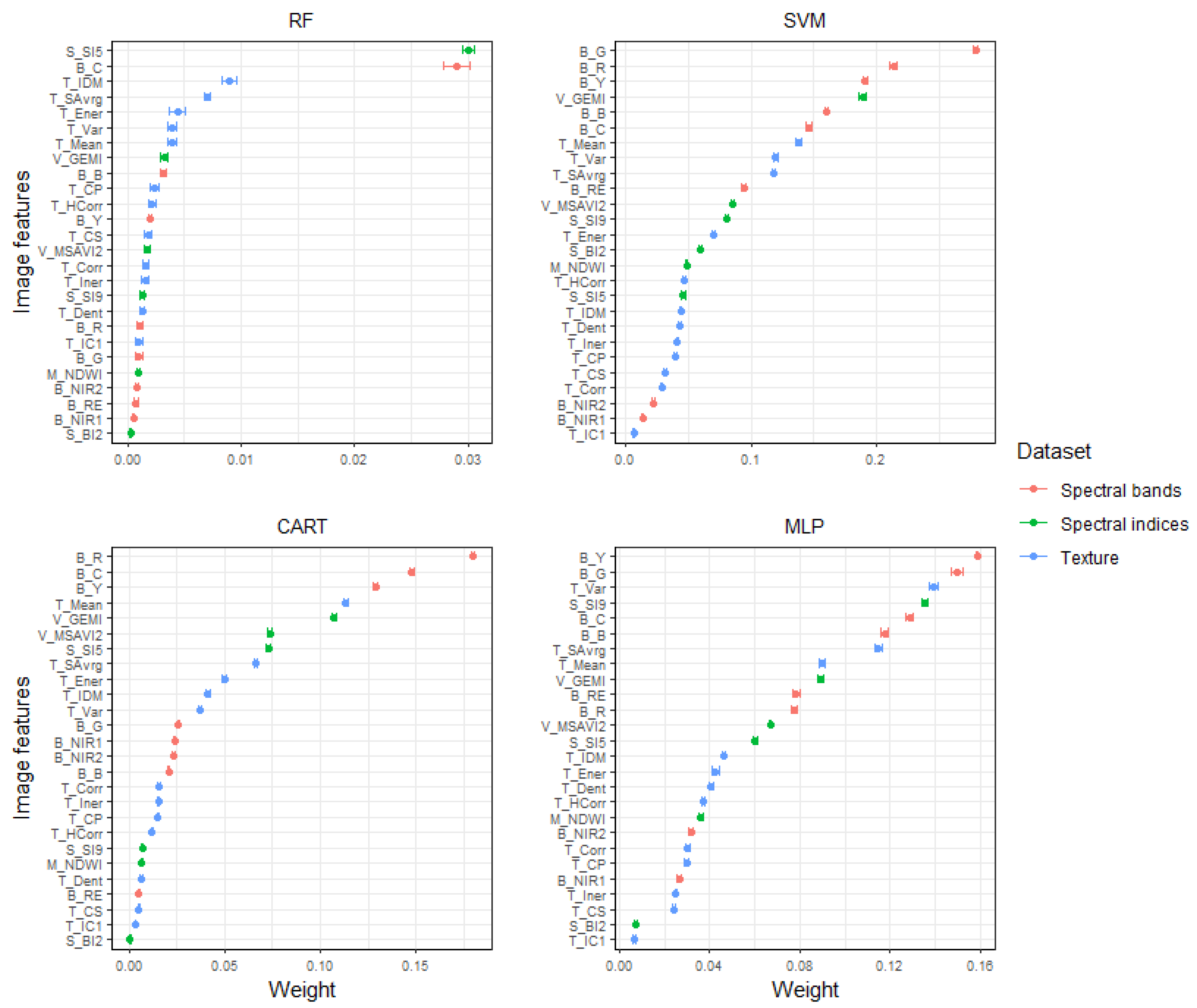
2.5. Feature Selection

Remote sensing image features such as spectral indices (vegetation, moisture and soil indices) as well as texture variables tend to exhibit high levels of collinearity. Highly correlated features increases data redundancy and risk of overfitting, which could have adverse consequences for algorithm performance especially for high-dimensional datasets [66], a problem that results from the Hughes phenomenon [67]. Although nonparametric machine learning algorithms are thought to be less susceptible to Hughes phenomenon, recent findings shows they benefit from dimensionality reduction nonetheless [68]. In our case, we aimed to target the most robust predictor set while reducing prohibitive computational efforts.
Image variables were selected by combining two procedures. First, we checked for collinearity with the Variance Inflation Factor (VIF) using the “usdm” package [69] within R-programming environment [70]. This was done separately for the spectral indices (i.e., vegetation, moisture and soil) and the Haralick texture features derived from the WorldView-3 imagery (see Table 3). VIF measures the degree to which predictor variables are correlated. For example, given k independent predictor variables, each variable is regressed with the remaining k 1 variables and coefficient of determination ( R 2 ) is estimated. The VIF of the dependent variable is thus computed as
V I F = 1 1 R 2
Large values of VIF implies a corresponding high degree of collinearity and vice versa. Following VIF analysis, correlated variables were subsequently removed by considering a stepwise elimination threshold of VIF 10 [71]. The VIF assessment resulted in six spectral indices and 15 Haralick texture features being retained.
Second, we combined the less correlated spectral indices and texture variables with the original image bands to select final image feature subset using Random Forest-Recursive Feature Elimination (RF-RFE) [72,73]. Recursive Feature Elimination (RFE) is an iterative process that uses some measure of feature importance to rank and select features by backward elimination [72]. The technique basically builds a model with the entire feature set, computes an importance score for each feature, removes the least important features and repeats the process until a user-defined number of features subset is reached. We used feature importance scores derived from random forest out-of-bag (OOB) error estimates for ranking features in the RF-RFE process. We then determined the final subset of features by analysing the relationship between number of features and accuracy scores derived from a stratified 10-fold cross-validation assessment. Overall, 26 WV-3 image features achieved optimal accuracy (See Supplementary Data in Appendix A). All steps in the RF-RFE process were implemented using Scikit-learn python library [74].

2.6. Machine Learning Algorithms

There is a proliferation of machine learning algorithms, which, coupled with the conflicting reports of their performance in remote sensing classification literature [75], makes it challenging to select the optimal method for any specific application. The optimal classification algorithm is generally context-specific and in most cases depends on the landscape and classes mapped [76], parameter settings [75,77,78], nature of training data [79,80,81,82] and data dimensionality [75,83]. Lawrence and Moran [76] recommend prior experimentation with multiple classifiers to determine optimal performance.
For this study, we tested four state-of-the-art nonparametric machine learning algorithms: Random Forest (RF) [27], Support Vector Machines (SVM) [28], Classification and Regression Trees (CART) [29] and Multilayer Perceptron (MLP) [30]. All have been shown to achieve high performance in many remote sensing applications, and in particular, land cover mapping [75]. Their superiority in handling complexity and high-dimensional data makes them ideal for application in highly heterogeneous savannah landscape conditions [23]. The selected algorithms were configured and implemented in the python programming environment using Scikit-learn python library [74]. Optimal parameter values (see in Table A10 in supplementary data, Appendix A) from hyperparameter tuning were used in each model. Summary descriptions of how the algorithms work are presented below.

2.6.1. RF

The RF classifier is an ensemble of decision tree algorithms with demonstrated robustness in remote sensing image classification compared to single classifiers [27,79]. The algorithm relies on unit vote contributions from each classifier within the ensemble to assign input vectors to different classes, where the most frequently voted class is retained [27]. The individual decision trees are parameterised using several independent random subsets of training data sampled through bootstrap aggregation or bagging. This reduces multicollinearity and generalization error [26,27]. The input vectors that do not form part of the bootstrap sample (i.e., “out-of-bag” (OOB) sample) are used for evaluation and variable importance estimation [27,84]. By design, decision tree classifiers require some measure for selecting suitable features per class, which maximizes dissimilarities between classes [79]. The RF algorithm uses Gini Index for feature selection at each node [85]. When assigning an input pixel to a class ( C i ), for a given training set (T), the Gini Index measures feature impurity with respect to the different classes and is expressed as
i j ( f ( C i , T ) / | T | ) ( f ( C j , T ) / | T | )
where ( f ( C i , T ) / | T | ) is the probability that the selected pixel belongs to class C i [79,86].
Each decision tree therefore grows to a maximum depth using a combination of features. The number of features used to grow a tree at each node and the number of decision trees are the required user-defined parameters to instantiate a RF prediction model [86].

2.6.2. SVM

SVM was developed based on statistical learning theory [87]. The algorithm creates an optimal separating hyperplane based on the location of a small subset of training samples at class boundaries, the so-called “support vectors” [28]. Given a simple binary linear classification problem, the SVM uses quadratic optimization techniques to select the optimum margin of separation between the two classes such that the distance to the hyperplane from the closest support vectors of both classes is maximal [28,82].
For a nonlinear classification problem, the algorithm selects the optimal margin by (i) allowing some misclassification errors and (ii) transforming the original input space into a higher dimensional feature space using nonlinear functions ϕ [87], making linear separation possible in the new feature space. To reduce computational cost, kernel functions, K ( x i , x j ) = ϕ ( x i ) · ϕ ( x j ) , such as polynomials, radial basis and sigmoid functions, are used for the transformation [88]. The decision function is given by
f ( x ) = s i g n i = 1 l α i y i ( ϕ ( x i ) · ϕ ( x j ) ) + b
where α i is a slack variable (Lagrange multiplier).
To classify new datasets, the algorithm uses learned parameters from the decision function based on training data. The trade-off between margin of class separation and misclassification errors is controlled by defining a regularisation parameter C , where C Z and 0 < C < [28].

2.6.3. CART

CART is a decision tree algorithm that builds classification or regression trees based on categorical or numerical attributes, respectively [85]. The structure of the tree is typified by a root node and a series of internal nodes (splits) and terminal nodes (leaves). Within this framework, the algorithm builds a model by recursively partitioning the training dataset into increasingly homogeneous subsets using tests applied at each node to training features [89]. Given a continuous data set, the test performed at each node is of the form
x i > c
for decision functions based on a single feature (i.e., univariate decision trees), where x i is a measurement in n feature space ( n = 1 in this case) and c is a decision threshold estimated from the range of x i measurements [90]. The threshold (c) value is determined using an impurity measure such as entropy [91] and the Gini index [85]. If the decision boundaries are defined by a combination of features (i.e., multivariate decision trees), the test takes the form
i = ln a i x i c
where a i is a vector of coefficients of a linear discriminant function estimated from the training data [90]. The series of testing outputs form the branches of the tree which proceeds sequentially through internal nodes until a terminal node is reached. At each terminal node, class labels are assigned based on maximum probabilities [92].

2.6.4. MLP

The MLP is a feedforward artificial neural network (ANN) classifier which is trained using back-propagation [93]. Learning in ANN is inspired by the functioning of neurons within the brain, which is based on parallel and distributed processing of information [94]. Similarly, the MLP architecture is composed of multiple layers of fully connected processing units called neurons, which are arranged sequentially as a network of input, hidden and output layers. During training, each unit in a hidden layer receives data from the input/previous layer, processes it and feeds it forward to units in the next layer [95]. This allows more abstract representations of the data to be learned until the output layer is reached [26]. The connections between units carry weights, which are modified iteratively to minimise a cost function. Apart from the input layer, the net input to each unit is therefore the weighted sum of outputs from the previous layer [94,95]. The net input is wrapped in an activation function to produce the output for that unit. The output for each processing unit is expressed as
o i = f j w i j o j + b i
where o i is the output of a neuron in layer i, w i j is the connecting weight between layers i and j, o i is output from layer j and b i is bias and f is the activation function [94,95].

2.7. Algorithm Calibration and Evaluation

The machine learning algorithms, namely, RF, SVM, CART and MLP, were first calibrated and evaluated for general land cover classification using data from a sub-area within the Lower Sabie landscape (see Figure 1) via a nested cross-validation approach. For each algorithm, the combination of parameters that returned the best expected classification accuracies were then used in the prediction of grazing lawn occurrence probabilities in the broader Lower Sabie and Satara Landscapes. The steps employed are broadly summarised into (i) data preparation, (ii) parameterisation training and classification and (iii) accuracy assessment. All processing was done using Intel(R) Core(TM) i5-6200U CPU with 8GB RAM on 64 bit Windows 10 operating system, and was supplemented by leveraging the power of Google’s free GPU hardware, using the Google Collaborator platform.

2.7.1. Data Preparation

We used the post-RF-RFE spectral and texture variables as input predictors for modelling. The input dataset was then transformed by subtracting the mean and scaling to a unit variance to generate normalised scores per feature using Equation (7):
z i j = x i j μ j σ j
where x i , μ j and σ j are pixel value, mean and standard deviation of pixels in the j t h feature, respectively, and z i j is the transformed value of x i j [96].
Normalising input features is a crucial preprocessing technique which approximately equalises dynamic data ranges in features for unbiased and improved learning [97]. Further, it is a common requirement prior to the training of machine learning estimators such as Support Vector Machines and Artificial Neural Networks [96].

2.7.2. Parameterisation, Training and Classification

Each of the selected algorithms comes with a set of hyperparameters which has to be tuned to maximise performance during training. Algorithm training thus involved hyperparameter optimisation whereby optimal hyperparameter sets were selected for RF, SVM, CART and MLP algorithms from a predefined grid (see Analysis Script in Appendix B). The optimisation process and selection of best model parameters were performed using randomised grid search in a 2 × 5 nested cross-validation approach with 10 iterations. Nested cross-validation incorporates optimal hyperparameter selection and unbiased estimation of model performance in inner and outer cross-validation loops respectively [98]. The approach is mostly recommended against traditional “flat cross-validation” which results in biased accuracy estimates due to information leakage and the split sample method plagued by insufficient availability of training and test datasets [99]. The chosen thresholds for tune-length and train–test splits were deemed appropriate to provide a reasonable trade-off between ensuring a robust model and computational time. Hyperparameters that returned the best expected classification accuracies were selected and used as input parameters in the machine learning algorithms. The algorithms were retrained with the full training data for landscape-wide prediction of land cover occurrence probabilities in both the Lower Sabie and Satara landscapes.
Individual image variable weights were computed using permutation feature importance estimates [74] in order to assess their relative contributions in each machine learning model. Permutation feature importance (PFI) generates variable weights based on an observed decrease in model score when a single variable is randomly shuffled [27]. The drop in model score thus represents the degree to which the model depends on the variable of interest. The PFI technique is model agnostic, which makes it suitable for comparison of feature importance estimates from RF, SVM, CART and MLP models used in this study.
The predicted occurrence probability surface for grazing lawns was selected and used as input in an optimised probability thresholding procedure. Optimised probability thresholding involved the selection of a single occurrence probability value (threshold) which maximises some measure of classification accuracy [100] for the target class. We tested a series of probability values at 0.05 intervals to determine the threshold that maximises F-score of grazing lawn detection. Grazing lawn (G) and non-grazing lawn (O) classes were assigned using simple relational expressions represented by Equation (8) and Equation (9), respectively,
G = p t
O = p < t
where p is occurrence probability and t is the optimal probability threshold, t p .

2.7.3. Accuracy Assessment and Comparison

Model performance in discriminating different savannah land cover types during hyperparameter tuning was assessed using point and interval estimates of Overall Accuracy (OA) and F-score, based on a 2 × 5 nested cross-validation approach (see Section 2.7.2). Further, accuracy of grazing lawn/non-grazing lawn binary maps was assessed by confusion matrix [101], from which precision, recall, F-score and OA metrics were calculated using Equations (10)–(13). Accuracy-adjusted estimates of grazing lawn area coverage were obtained following Olofsson et al. [102].
P r e c i s i o n = t p t p + f p
R e c a l l = t p t p + f n
F s c o r e = 2 P r e c i s i o n R e c a l l P r e c i s i o n + R e c a l l
O A = t p + t n t p + f p + t n + f n
where tp, fp, tn and fn represent the number of true positive, false positive, true negative and false negative cases, respectively.
Marginal homogeneity between predictions from model pairs was tested at 5% level of significance using the McNemar chi-squared ( χ 2 ) test [103]. The McNemar test compares the error matrices of two classification methods to test the null hypothesis that the two methods have the same error rate. The method is based on χ 2 -test and provides a robust statistical comparison of class-wise predictions between two algorithms [104]. Additionally, the estimated proportion of grazing lawn cover (PGLC) was compared for model pairs using the two-proportion Z-test at 5% level of significance. The two-proportion Z-test follows a χ 2 distribution with one degree of freedom [26], and was used to test the null hypothesis of no difference between PGLC for model pairs.

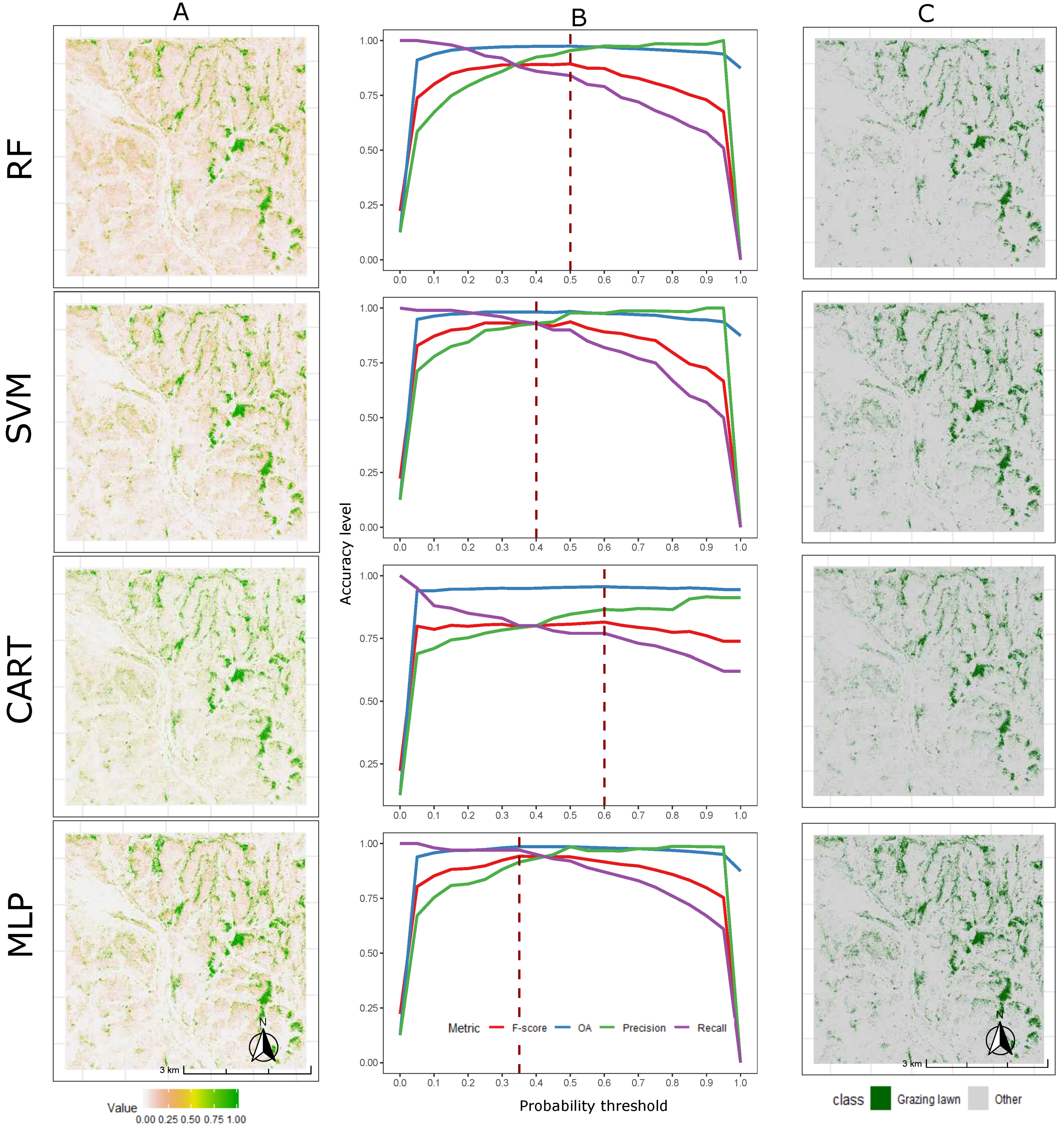
2.8. Spatial Analysis of Grazing Lawn Distribution
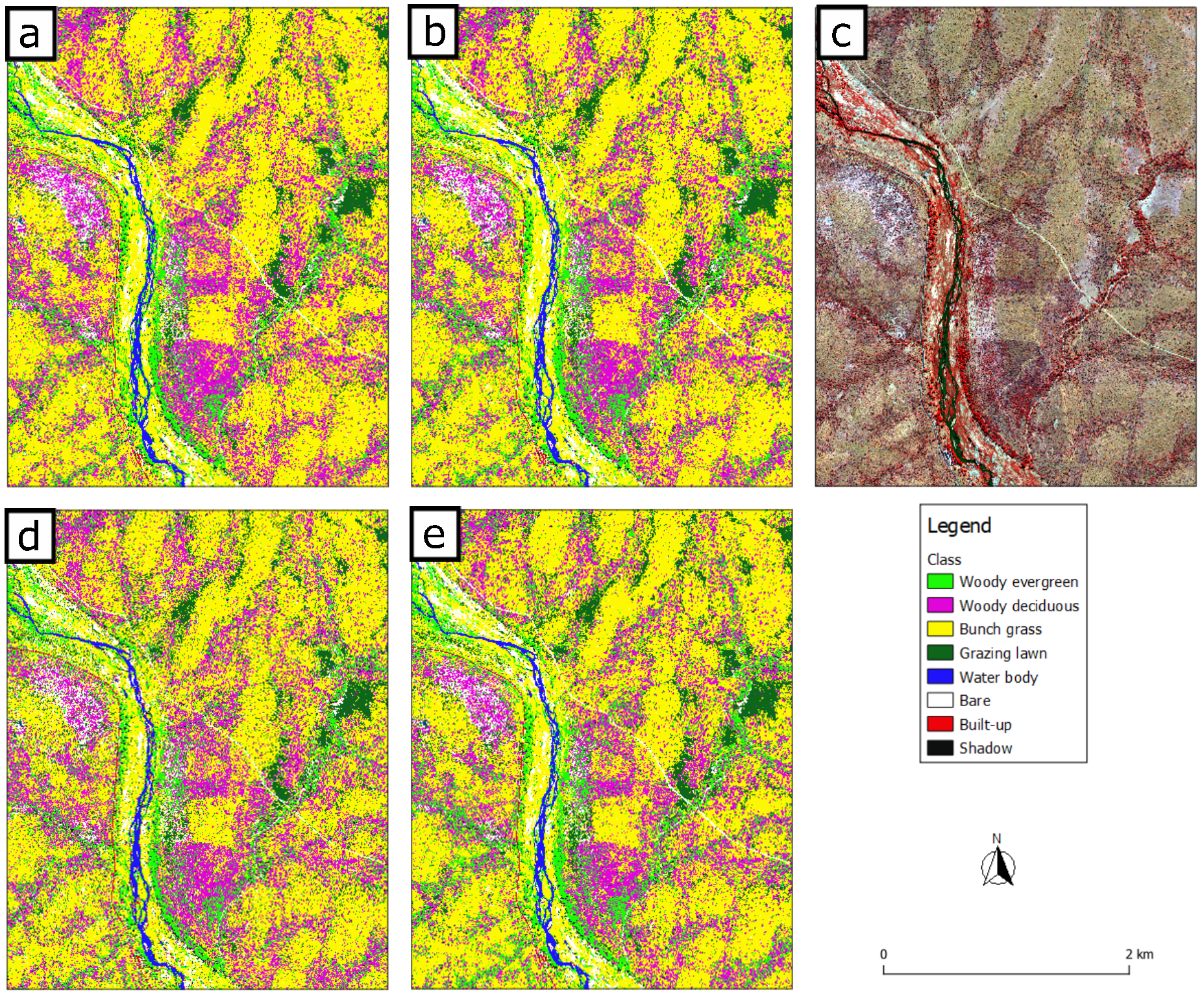
Using spatial metrics, we determined characteristics of grazing lawn distribution at landscape-scale and analysed spatial patterns along a gradient of distance from water source in both Lower Sabie and Satara landscapes. Spatial metrics provide vital information on landscape configuration and composition [105]. Spatial-contextual information such as density, shape, size and aggregation of land cover patches can be extracted from spatial metrics to better understand ecological processes at the landscape-scale [105,106]. The classification output with the least error properties was selected as input in the calculation of (i) Number of Patches (NP), (ii) proportion of landscape covered by grazing lawns (PL), (iii) maximum patch area (MPA) and (iv) cohesion index (CI) [106], from which patterns in grazing lawn structure were determined. Further, Pearson’s correlation and coefficients of determination were estimated in order to identify the nature and significance of the relationship between grazing lawn structural attributes and proximity to water source. Calculation of the selected spatial metrics was carried out using the “SpatialEco” package [107] in the R programming environment [70].

3. Results

3.1. Model Quality for Land Cover Classification

Cross-validation accuracy results for individual models using F-score and Overall Accuracy (OA) measures are presented in Table 4. Generally, all models achieved high accuracies in differentiating the different land cover classes, with median F-score and OA measures ranging between 92.75 ± 0.005 % and 95.73 ± 0.003 % and 90.92 ± 0.002 % and 94.27 ± 0.003 % , respectively. RF, SVM and MLP models had similar accuracy scores and marginally outperformed CART for both F1 and OA measures (Table 4).
Figure 5 shows land cover maps for the training region at 2 m spatial resolution. The maps show similar representation of savannah land cover types across all models, all of which were closely consistent with the reference satellite image scene (Figure 5c).
Figure 6 shows permutation feature importance estimates across all models. A mix of image features from original spectral bands, spectral indices and texture variables showed high importance in each model. There was generally more agreement among SVM, CART and MLP models in assigning relatively more importance to original spectral bands in terms of both magnitude of feature weight and number of features. However, image features that exhibited high importance in the RF model were largely dominated by texture variables (Figure 6). Image features that were of highest importance in RF, SVM, CART and MLP models were S_SI5, B_G, B_R and B_Y, respectively.
A summary of the most important predictors for each feature group (i.e., spectral bands, spectral indices and texture variables) is presented in Table 5. We concur with the authors of [108] that identification of the most important image features considers both the magnitude of feature weights and consistency of being assigned high importance across all models. In terms of magnitude, image features that were considered highly important in each model were limited to the first three features, in each feature group (Figure 6). Conversely, features were deemed consistent if they were assigned high importance in at least three models (Table 5). Among the most important image features were B_C and B_Y for spectral bands, V_GEMI and V_MSAVI2 for spectral indices and T_Mean and T_SAvrg for texture variables (see Table 5 for features in bold).

3.2. Grazing Lawn Occurrence Probability Prediction and Classification

The outputs of grazing lawn occurrence probability surfaces for RF, SVM, CART and MLP models are shown in Figure 7A and Figure 8A for Lower Sabie and Satara landscapes respectively. The general pattern of grazing lawn occurrence probability surfaces at both study sites is comparable among the four models. Within the Lower Sabie site, high grazing lawn occurrence probabilities were mostly confined to the eastern and north-eastern part of the landscape, and were similar across all models (Figure 7A). The obvious qualitative difference among models is the relative lack of many very low values in the CART probability surface compared to RF, SVM and MLP models.
Within the Satara landscape, high grazing lawn occurrence probabilities mostly aligned along a diagonal stretch from northwest to southeast (Figure 8A), which is the interface of the granite and basalt geologies. Despite similarities in spatial distribution of high occurrence probability values, there were noticeable qualitative differences in range among the four models. The RF probability surface exhibited a relatively high prevalence of a continuous range of very low to medium probability values across the landscape, and very few distinctively high occurrence probabilities. In contrast, the CART model predicted relatively more medium to high probability values across the landscape, while MLP and SVM predictions were similar in the distribution of very low and very high occurrence probability values (Figure 8A).
Plots of model F-score, Precision, Recall and OA values generated over a series of predicted probabilities for the Lower Sabie and Satara landscapes are presented in Figure 7B and Figure 8B, respectively. Analysis of the relationship between F-score and predicted probabilities revealed the optimal threshold for classifying grazing lawns. The optimal threshold is the probability value which maximises model F-score of grazing lawn detection, and was found to coincide with or lie close to the equilibrium point between model Precision and Recall. The resulting values varied across models, with the F-score of RF, SVM, CART and MLP models peaking at 0.5, 0.4, 0.6 and 0.35, respectively, for Lower Sabie as seen in Figure 7B. Similar analysis on predicted probability surfaces for the Satara landscape resulted in relatively lower thresholds for RF, SVM and CART (0.35, 0.25 and 0.35, respectively) and a higher threshold for MLP (0.6) where model F-scores were maximum Figure 8B.
The grazing lawn/non-grazing lawn binary maps resulting from applying corresponding thresholds to each of the four predicted probability surfaces are shown in Figure 7C and Figure 8C for both Lower Sabie and Satara landscapes, respectively. Analogous to the probability surfaces, patterns of grazing lawn distribution were similar for all classifications within both landscapes. However, local variations persisted and were consistent with the distribution of predicted probability values for each model in both landscapes. Overall, the Satara maps showed a considerable level of speckling (Figure 8C).
A summary of accuracy measures for grazing lawn detection is presented in Table 6. F-scores for Lower Sabie ranged between 0.81 for CART to 0.94 for MLP, while SVM and RF classifications achieved F-score of 0.93 and 0.89 respectively (Table 6). Grazing lawn detection accuracy results were high, but relatively lower for the Satara area compared to Lower Sabie. F-score ranged between 0.75 for CART to 0.88 for SVM, while RF and MLP achieved F-scores of 0.87 and 0.85, respectively (Table 6).
Accuracy-adjusted estimates of area covered by grazing lawns within both landscapes are presented in Table 7. As expected, all model classifications gave comparable estimates of grazing lawn cover within the Lower Sabie site, ranging between 2.46 km2 (for RF) and 2.98 km2 (for CART) (Table 7). In contrast, estimates of grazing lawn cover were significantly different ( p 0.05 ) for all models within the Satara landscape (see test results in Table A1 of supplementary data).
McNemar test results presented in Table 8 showed statistically significant differences ( p 0.05 ) in grazing lawn detection error rate when comparing CART to RF, SVM and MLP models in both Lower Sabie and Satara landscapes. In contrast, no significant differences were observed for all the other model pairs (Table 8).

3.3. Spatial Patterns in Grazing Lawn Cover

Landscape-scale summary of number of grazing lawn patches, total coverage, connectedness and patch size distribution are presented in Figure 9.
Number of grazing lawn patches was relatively higher in Lower Sabie compared to the Satara landscape (Figure 9A). However, analysis of patch size distribution revealed the Satara landscape as having relatively larger grazing lawn patches (Figure 9D), and higher area coverage compared to the Lower Sabie landscape (Figure 9B). Spatial connectedness of grazing lawn patches was however comparable in both landscapes (Figure 9C).
Further analysis of patterns in the proportion of landscape covered by grazing lawns (PL), maximum patch area (MPA) and cohesion (CI) revealed significant relationships with distance from water sources in both landscapes. Grazing lawn PL, MPA and CI showed an inverse relationship with distance from water source in both landscapes (see correlation coefficients in Table 9). However, the trends were relatively less distinct in the Lower Sabie landscape (Figure 10), as also suggested by the differences in magnitude of correlation coefficients between both landscapes (Table 9). Overall, grazing lawn fractional cover, patch size and spatial connectedness were highest within 0.7 km from water sources in both Lower Sabie and Satara landscapes (Figure 10).

4. Discussion

4.1. Model Quality for Savannah Land Cover Classification

In this study, efforts were focused on developing robust machine learning framework for grazing lawn detection by first assessing model performance for general classification of savannah land cover types. The convergence of remote sensing and data science techniques through machine learning offers unparalleled capacity for more accurate processing of satellite imagery, especially for the purposes of land cover monitoring. While this presents many advantages for remote sensing-based ecosystem monitoring, the choice of fit-for-purpose machine learning algorithms often requires some experimentation. This is partly due to the vast availability of options to select from, but most importantly also due to contextual differences in application such as varying landscape conditions, data and research objectives [76,82]. Robust evaluation of algorithm performance is therefore vital for the selection of optimal models for application. The nested cross-validation approach used here allowed the simultaneous tuning of hyperparameters and unbiased estimation of individual model performance. In so doing, the optimum combination of algorithm hyperparameters which enhanced model quality could be selected. Model quality evaluation via nested cross-validation has been proven effective in avoiding biased accuracy estimates common in “flat cross-validation” due to information leakage, while preventing poor model generalisation capabilities due to data paucity—a regular challenge of the split sample approach to model evaluation [99].
All machine learning models (RF, SVM, CART and MLP) demonstrated high performance in classifying the different savannah land cover categories. Even so, RF, SVM and MLP marginally outperformed the CART model. The relatively lower performance of CART observed in this study is consistent with widely reported inferiority of single decision tree (DT)-based classifiers relative to other machine learning algorithms for land cover classification [23,31,109]. For example, similar findings were reported by Kaszta et al. [23] in a comparative assessment of classification algorithms for seasonal separation of southern African savannah components. The authors recorded CART as having the lowest accuracy score in both pixel-based and object-based approaches relative to SVM and RF algorithms. Camargo et al. [31] compared the performance of RF, SVM, MLP and DT for classifying the Brazilian tropical savannah biome, and found that DT produced a relatively lower performance than RF, SVM and MLP classifiers. Similar to our findings, the authors recorded closely comparable performance for the latter three algorithms. In a related Mediterranean land cover monitoring study, Rodriguez-Galiano and Chica-Rivas [109] reported significantly lower mapping accuracy for DT than SVM, ANN and RF algorithms.
Although CART is relatively more flexible and intuitive to implement, it is very sensitive to small variability in data, which, in this case, may have contributed to the relatively lower performance in a heterogeneous savannah landscape. Compared to single decision trees such as CART, the RF algorithm draws its higher generalisability from the contribution of multiple decision trees parameterised using random subsets and bootstrap aggregation [27]. RF is therefore highly adaptable to different data ranges and robust against multicollinearity. Similarly, the MLP architecture allows more abstract representations of data to be learned [95]. However, the performance of MLP is strongly influenced by input data structure, and performs better when data ranges of all input features are equal [96]. Thus, the inclusion of data normalisation during preprocessing likely aided gains in classification accuracy. In the case of SVM, the use of nonlinear vector mapping functions facilitates creation of decision boundaries for effectively dealing with nonlinearly separable classes [88]. The superiority of RF, MLP and SVM algorithms in dealing with the typical spectral homogeneity of the heterogeneous savannah landscape could thus be attributed to their relatively higher adaptive capacity in complex nonlinear classification problems. It should be noted that RF was used in an RF-RFE procedure for selecting final input image features for classification (see Section 2.5). This may have aided the performance of RF, although the RF-RFE algorithm was configured with different (default) hyperparameters during implementation.
As expected, a combination of original image bands, spectral indices and texture variables enhanced discrimination capacities of the machine learning models in savannah land cover classification. Across all models, the most important predictors—B_C, B_Y (original bands), V_GEMI, V_MSAVI2 (spectral indices), T_Mean and T_SAvrg (texture features)—highlight variations in photosynthetic status and structure of savannah vegetation. The high importance of the coastal blue (B_C) and yellow (B_Y) WorldView-3 image bands could be attributed to their strong sensitivity to differences in foliar chrolophyll content [24], given that images were acquired in the dry season, which is when phenological differences are most pronounced [32,45]. Several studies have reported the contribution of these bands and the red edge band in mapping vegetation components [23,110,111]. Unlike the reported studies, the red edge band was not very important in our classification of savannah land cover. The coastal blue wavelength is absorbed by chlorophyll in healthy plants while the yellow band detects dryness/“yellowness” of vegetation, both of which are instrumental in vegetative analysis. The high importance of the spectral indices could be explained by their strong correlation with vegetation biomass [56,57] and moisture content [58,59], which helps to capture the varying characteristics of heterogeneous savannah vegetation that would otherwise be attenuated when using the original image bands alone. Additionally, the high importance of the texture features highlighted the chromatic variations in dry season savannah vegetation components. Both T_Mean and T_SAvrg measures inter-pixel average in brightness values which were sufficiently captured at 2 m resolution of the WorldView-3 in a heterogeneous savannah landscape.

4.2. Grazing Lawn Detection and Model Comparison

After ascertaining the optimal parameters for training, models were refitted with the entire training set for wide-scale prediction of land cover occurrence probabilities in both Lower Sabie and Satara landscapes. For each landscape, the general pattern of grazing lawn occurrence probabilities was comparable for all models, particularly the distribution of high occurrence probability values. Individual model outputs however exhibited local predictive variations in the distribution of low to medium occurrence probabilities, which could be reflective of differences in model complexity and uncertainties [112,113]. Binary maps were derived from predicted grazing lawn occurrence probability surfaces using thresholds which maximised F-score. Hird et al. [100] adopted a similar approach for large area classification of wetlands and drylands using True Skill Statistics (TSS), and achieved 85% OA score. As expected, derived maps showed more coherent representation of grazing lawn areas within the Lower Sabie landscape, while maps for the Satara landscape were characterised by relatively higher degree of noise, particularly for the CART-derived map. This was also reflected in F-score measures, where relatively higher grazing lawn detection accuracies were recorded across all models for the Lower Sabie savannah landscape. It should be emphasised that models were trained using data from the Lower Sabie landscape—for reasons related to training data quality and computational cost—which allowed testing their spatial transferability. Possible differences in dry season reflectances due to the different rainfall regimes and underlying geologies as well as difference in image acquisition geometries, may have increased prediction bias of model spatial transfer and contributed to the observed differences both across the different landscapes and models. Further analysis is required to comprehensively ascertain the impacts of differences in environmental conditions and image acquisition characteristics on spatial transferability of the classification models. McMenar and two-proportion Z-test results showed significant differences ( p 0.05 ) in error rates for pairs of of CART versus other models, further highlighting the relative preponderance of RF, SVM and MLP. Overall, differences in accuracy of grazing lawn detection were attenuated when models were applied in a different spatial context. This suggests the need to calibrate predictive models with local contextual information prior to application. Additionally, our findings re-emphasise recommendations from [114,115,116] to conduct statistically rigorous comparison of accuracy statements before drawing definitive conclusions on map quality assessment.

4.3. Spatial Patterns in Grazing Lawn Distribution

The formation and persistence of grazing lawns in southern African savannah landscapes has been identified to be dependent on a number of interacting top-down and bottom-up ecological processes. Among the most widely reported are continued grazing [4,117], which can be linked to fire, rainfall and nutrient hotspots concentrating grazers on specific areas [11,12,13]. Spatial variations in such factors are thus expected to shape spatial patterns and distribution of grazing lawns [10].
Both fire and grazers consume grass biomass, and have the potential to shift grass communities into tall grass or short grass grazing lawn states [11]. However, the rate at which these alternate grassland states are established is strongly influenced by landscape productivity [12]. Tall grasses are strong light competitors and are well adapted to fire-prone conditions due to their extensive rooting system, which makes them the dominant grass community under high productivity conditions [10]. On the other hand, short grass grazing lawns can withstand high grazing pressure due to their stoloniferous growth form which protect reproductive parts from being destroyed. Subject to similar grazing conditions, the proportion of grazing lawn cover within the savannah landscape is expected to be lower under high rainfall regimes. This is consistent with the relatively high grazing lawn coverage in the semiarid Satara landscape compared to the mesic Lower Sabie landscape.
Different parts of the savannah landscape may be predisposed to grazing lawn formation due to the presence of resource hot-spots that attract grazers [10]. This study explored the relationship between water sources as resource hot-spots and patterns in grazing lawn distribution. Grazing lawn structural attributes expressed as fractional cover (PL), maximum patch area (MPA) and connectivity (CI) were examined relative to distance from water sources. Generally, patterns in grazing lawn structure significantly correlated with distance from water sources, and was similar in both mesic and semiarid landscapes. The largest contiguous grazing lawn patches were found within 0.7 km from water sources, which is suggestive of the prevalence of grazing lawns in close proximity to waterbodies. This could be attributed to increased grazer activity around water sources [49,118] and is consistent with observations that landscape-scale distribution of grazers is generally biased towards areas around reliable rivers and permanent waterholes [49,119]. For example, Smit [118] found that different grazers of varying body mass and digestive requirements had significantly strong association with both rivers and artificial waterholes in Kruger National Park. This phenomenon is especially evident during dry seasons when moisture content of graze is low [120] and surface water is spatially restricted [119]. Additionally, sodic sites which are highly utilised by grazers and hence have extensive grazing lawn cover, occur close to waterbodies and drainage lines, and may have contributed to the observed patterns.
It is important to note that other landscape phenomena may be influencing spatial patterns in grazing lawn distribution. For example, the prevalence of open grasslands, which is typical of the Satara landscape, may lead to the formation of more grazing lawn patches. Burkepile et al. [121] found that more open savannah grasslands with sparse woody cover make attractive habitats or grazing grounds for selection by herbivores such as zebra (Equus quagga) and blue wildebeest (Connochaetes taurinus), in part to mitigate the risk of predation.

5. Conclusions

Dynamics in grazing lawn communities in southern African savannahs have been directly linked with fluctuations in mega-herbivore densities and changing fire regimes, with cascading effects on ecological processes such as nutrient cycling, plant community composition and habitat structure. Knowledge of their coverage and distribution is therefore critical to understanding habitat heterogeneity and the overall ecology of these vital grassland systems. This study presents the first attempt to develop a broad-scale approach for grazing lawn detection using very high-resolution satellite images. We demonstrated the successful application of machine learning techniques for mapping grazing lawn occurrence from WorldView-3 satellite imagery, and further analysed their spatial structure and distribution in southern African savannahs. The RF, SVM and MLP models produced comparable accuracies in the classification of different plant functional types (PFTs) and other land cover, all of which outperformed the CART model. Differences in grazing lawn detection accuracy followed a similar trend particularly within the same landscape (Lower Sabie). Performance for all models however reduced when they were transferred to a different landscape (Satara) even though high accuracies were achieved. Analysis of grazing lawn spatial structure and distribution showed that the Satara savannah landscape supports a relatively higher proportion of grazing lawn cover than Lower Sabie. Additionally, larger and contiguous patches persist in close proximity to water sources, which concentrate grazers within the savannah landscape, irrespective of differences in underlying environmental conditions. The proposed approach provides a novel and robust workflow for accurate and consistent landscape-scale monitoring of grazing lawns. Additionally, our findings ascertain experimental and local-scale reports on grazing lawn dynamics at a wider landscape scale, and provide timely information critical for understanding habitat heterogeneity in southern African savannahs.

Author Contributions

Conceptualization, K.T.A. and P.A.; Data curation, K.T.A.; Formal analysis, K.T.A.; Methodology, K.T.A.; Project administration, K.T.A., P.A. and I.P.; Software, K.T.A.; Supervision, P.A., C.G.M., I.P. and I.P.J.S.; Writing—original draft, K.T.A.; Writing—review and editing, K.T.A., P.A., C.G.M., I.P. and I.P.J.S. All authors have read and agreed to the published version of the manuscript.

Funding

The Department of Geography and Geology, Edge Hill University, provided funding for this study. Field work was supported by the 2019 Geographical Club Award with grant reference GCA 42/19, offered by the Royal Geographical Society (RGS_IBG).

Acknowledgments

Great thanks to former colleague, Daniel Knight for his immense help in field data collection. We are grateful to South Africa National Parks (SANParks) Scientific Services for the initial comments on the project proposal, which helped shape the focus of this study. We would like to sincerely thank Corli Wigley-Coetsee, Samantha Mabuza and Obert Mathebula for providing logistical and administrative support during our field stay in KNP. We are also immensely grateful to our game guards Martin Sarela and Annoit Mashele.

Conflicts of Interest

The authors declare no conflict of interest.

Appendix A. Supplementary Data

Appendix A.1. Multicollinearity and Feature Selection

Multicollinearity analysis among derived image features showed that spectral indices exhibited higher correlation than texture features based on a stepwise elimination threshold of VIF ≥ 10. Twenty-one out of the 27 spectral indices (i.e., vegetation, moisture and soil combined) had collinearity problems. After eliminating the collinear variables, VIF values of retained spectral indices ranged from 1.19 to 3.94 (Figure A2A) with linear correlation coefficients between −0.002 (S_SI9∼M_NDWI) and −0.666 (S_SI9∼S_SI5). In contrast, only three out of the 18 texture features exhibited collinearity. The retained texture variables had VIF values ranging from 1.00 to 9.22 (Figure A2B) and linear correlation coefficients ranging between 6.14 × 10 5 (T_Dent∼T_Diss) and 0.79 (T_IDM∼T_Ener). Overall, six spectral indices (three soil indices, two vegetation indices and one moisture index) and 15 texture features (seven simple and eight advanced Haralick features) were retained (Figure A2A,B) and combined with the eight original image bands for final feature selection.
Figure A1. Plot of accuracy versus number of features.
Remotesensing 12 03357 g0a1
Figure A2. Feature selection results from VIF and RF-RFE analysis. (A) VIF of selected spectral indices. (B) VIF of selected texture features. (C) Importance scores of final selected image features following RF-RFE. Original bands and selected spectral indices and texture features from VIF served as input to RF-RFE. Final selection was based on number of features that retained optimal accuracy.
Remotesensing 12 03357 g0a2
Selection of final input image features was conducted using Random Forest Feature Elimination (RF-RFE). The RF-RFE procedure resulted in 26 image features (Figure A1) comprising of eight image bands, six spectral indices and twelve texture features. Figure A2C shows the relative importance scores of selected final input features in differentiating the different land cover categories (Table 1). The first 13 (50%) most important features were dominated by nearly equal proportions of spectral bands and spectral indices (six and five, respectively), with two texture features, while the remaining features were largely composed of texture variables (Figure A2C). Amongst the original bands, variables that exhibited high importance were B_C, B_R and B_Y. V_MSAVI2, S_SI5 and V_GEMI were the spectral indices of high importance, and the most influential texture variables included T_Ener and T_Mean.

Appendix A.2. Comparison of Grazing Lawn Area Estimates across Models in Each Landscape

Table A1. Two-proportions Z-test comparing the proportions of estimated grazing lawn cover. Values in parenthesis represent p-value. Model pairs that show statistically significant difference ( p 0.05 ) in proportion of grazing lawn cover are in bold. CART = Classification and Regression Trees, MLP = Multilayer Perceptron, RF = Random Forest, SVM = Support Vector Machines.
Lower SabieSatara
Model Pair χ 2 -testModel Pair χ 2 -test
CART v MLP0.000(1.00)CART v MLP5.017(0.025)
CART v RF0.000(1.00)CART v RF8.328(0.003)
CART v SVM0.000(1.00)CART v SVM7.225(0.007)
MLP v RF0.000(1.00)MLP v RF13.146(0.000)
MLP v SVM0.000(1.00)MLP v SVM11.657(0.000)
RF v SVM0.000(1.00)RF v SVM10.083(0.001)

Appendix A.3. Confusion Matrices for the Lower Sabie Landscape

Table A2. Confusion matrix summarising results from Random Forest (RF) model classification of grazing lawn and other cover.
RF
Reference ClassCommission Error (%)
Grazing lawnOther
Predicted ClassGrazing lawn841616.00
Other46930.57
Omission Error (%)4.552.26
Table A3. Confusion matrix summarising results from Support Vector Machines (SVM) model classification of grazing lawn and other cover.
SVM
Reference ClassCommission Error (%)
Grazing lawnOther
Predicted ClassGrazing lawn9377.00
Other76901.00
Omission Error (%)7.001.00
Table A4. Confusion matrix summarising results from Classification and Regression Trees (CART) model classification of grazing lawn and other cover.
CART
Reference ClassCommission Error (%)
Grazing lawnOther
Predicted ClassGrazing lawn772323.00
Other126851.72
Omission Error (%)13.483.25
Table A5. Confusion matrix summarising results from Multilayer Perceptron (MLP) model classification of grazing lawn and other cover.
MLP
Reference ClassCommission Error (%)
Grazing lawnOther
Predicted ClassGrazing lawn9733.00
Other96881.29
Omission Error (%)8.490.43

Appendix A.4. Confusion Matrices for the Satara Landscape

Table A6. Confusion matrix summarising results from Random Forest (RF) model classification of grazing lawn and other cover.
RF
Reference ClassCommission Error (%)
Grazing lawnOther
Predicted ClassGrazing lawn901312.62
Other125112.29
Omission Error (%)11.762.48
Table A7. Confusion matrix summarising results from Support Vector Machines (SVM) model classification of grazing lawn and other cover.
SVM
Reference ClassCommission Error (%)
Grazing lawnOther
Predicted ClassGrazing lawn93109.71
Other145092.68
Omission Error (%)13.081.93
Table A8. Confusion matrix summarising results from Classification and Regression Trees (CART) model classification of grazing lawn and other cover.
CART
Reference ClassCommission Error (%)
Grazing lawnOther
Predicted ClassGrazing lawn782524.27
Other254984.78
Omission Error (%)24.274.78
Table A9. Confusion matrix summarising results from Multilayer Peceptron (MLP) model classification of grazing lawn and other cover.
MLP
Reference ClassCommission Error (%)
Grazing lawnOther
Predicted ClassGrazing lawn881514.56
Other165073.06
Omission Error (%)15.382.87

Appendix A.5. Final Model Hyperparameters

Table A10. Results of optimal hyperparameter values used in each model, from 2 × 5 nested cross-validation using Scikit Learn python package. Refer to the work in [74] for more details on model hyperparameters.
ModelOptimal Hyper-Parameter ValueDescription
RFn_estimators = 2000,
max_features = ‘auto’,
max_depth = 20,
min_samples_split = 2,
min_samples_leaf = 1
n_estimators = number of trees in the forest.
max_features = number of features to consider for the split, ‘auto’ takes N o . f e a t u r e s .
max_depth = maximum depth of the tree.
min_samples_split = minimum number of samples required to split an internal node.
min_samples_leaf = minimum number of samples required to be at a leaf node.
MLPhidden_layer_sizes = (150,100,50),
activation = ‘logistic’,
solver = ‘adam’,
max_iter = 100,
alpha = 0.0000001
hidden_layer_sizes = number of neurons in each hidden layer (three layers in this case).
activation = activation function of the hidden layer.
solver = solver for weight optimization, ‘adam’ is based on the stochastic gradient optimizer.
max_iter = maximum number of iterations.
alpha = regularization parameter.
CARTcriterion = ‘gini’,
max_depth = 80,
min_samples_split = 20,
min_samples_leaf = 5
criterion = function to measure quality of split.
max_depth = maximum depth of tree.
min_samples_split = minimum number of samples required to split an internal node.
min_samples_leaf = minimum number of samples required to be at a leaf node.
SVMC = 1000,
gamma = 0.001,
kernel = ‘rbf’
C = regularization parameter.
gamma = kernel coefficient.
kernel = kernel type used, ‘rbf’ represents radial basis function.

Appendix B. Analysis Script

References

  1. Sankaran, M.; Ratnam, J.; Hanan, N. Woody cover in African savannas: The role of resources, fire and herbivory. Glob. Ecol. Biogeogr. 2008, 17, 236–245. [Google Scholar] [CrossRef]
  2. Shorrocks, B.; Bates, W. The Biology of African Savannahs; Oxford University Press: Oxford, MS, USA, 2015. [Google Scholar]
  3. Cromsigt, J.P.; Kuijper, D.P. Revisiting the browsing lawn concept: Evolutionary Interactions or pruning herbivores? Perspect. Plant Ecol. Evol. Syst. 2011, 13, 207–215. [Google Scholar] [CrossRef]
  4. Cromsigt, J.P.; Olff, H. Dynamics of grazing lawn formation: An experimental test of the role of scale-dependent processes. Oikos 2008, 117, 1444–1452. [Google Scholar] [CrossRef] [Green Version]
  5. Owen-Smith, N. Pleistocene extinctions: The pivotal role of megaherbivores. Paleobiology 1987, 13, 351–362. [Google Scholar] [CrossRef]
  6. Cromsigt, J.P.; te Beest, M. Restoration of a megaherbivore: Landscape-level impacts of white rhinoceros in Kruger National Park, South Africa. J. Ecol. 2014, 102, 566–575. [Google Scholar] [CrossRef] [Green Version]
  7. Waldram, M.S.; Bond, W.J.; Stock, W.D. Ecological engineering by a mega-grazer: White rhino impacts on a South African savanna. Ecosystems 2008, 11, 101–112. [Google Scholar] [CrossRef]
  8. Gill, J.L.; Williams, J.W.; Jackson, S.T.; Lininger, K.B.; Robinson, G.S. Pleistocene megafaunal collapse, novel plant communities, and enhanced fire regimes in North America. Science 2009, 326, 1100–1103. [Google Scholar] [CrossRef] [Green Version]
  9. Owen-Smith, R.N. Megaherbivores. The influence of very large body size on ecology. In Megaherbivores: The Influence of Very Large Body Size on Ecology; Cambridge University Press: Cambridge, UK, 1992. [Google Scholar]
  10. Hempson, G.P.; Archibald, S.; Bond, W.J.; Ellis, R.P.; Grant, C.C.; Kruger, F.J.; Kruger, L.M.; Moxley, C.; Owen-Smith, N.; Peel, M.J.; et al. Ecology of grazing lawns in Africa. Biol. Rev. 2015, 90, 979–994. [Google Scholar] [CrossRef]
  11. Donaldson, J.E.; Archibald, S.; Govender, N.; Pollard, D.; Luhdo, Z.; Parr, C.L. Ecological engineering through fire-herbivory feedbacks drives the formation of savanna grazing lawns. J. Appl. Ecol. 2018, 55, 225–235. [Google Scholar] [CrossRef] [Green Version]
  12. Archibald, S.; Bond, W.; Stock, W.; Fairbanks, D. Shaping the landscape: Fire–grazer interactions in an African savanna. Ecol. Appl. 2005, 15, 96–109. [Google Scholar] [CrossRef]
  13. Archibald, S. African grazing lawns—How fire, rainfall, and grazer numbers interact to affect grass community states. J. Wildl. Manag. 2008, 72, 492–501. [Google Scholar] [CrossRef]
  14. Veldhuis, M.P.; Fakkert, H.F.; Berg, M.P.; Olff, H. Grassland structural heterogeneity in a savanna is driven more by productivity differences than by consumption differences between lawn and bunch grasses. Oecologia 2016, 182, 841–853. [Google Scholar] [CrossRef] [PubMed] [Green Version]
  15. Leonard, S.; Kirkpatrick, J.; Marsden-Smedley, J. Variation in the effects of vertebrate grazing on fire potential between grassland structural types. J. Appl. Ecol. 2010, 47, 876–883. [Google Scholar] [CrossRef]
  16. Helman, D.; Lensky, I.M.; Tessler, N.; Osem, Y. A phenology-based method for monitoring woody and herbaceous vegetation in Mediterranean forests from NDVI time series. Remote Sens. 2015, 7, 12314–12335. [Google Scholar] [CrossRef] [Green Version]
  17. Marston, C.G.; Aplin, P.; Wilkinson, D.M.; Field, R.; O’Regan, H.J. Scrubbing up: Multi-scale investigation of woody encroachment in a southern African savannah. Remote Sens. 2017, 9, 419. [Google Scholar] [CrossRef] [Green Version]
  18. Jensen, J.R. Introductory Digital Image Processing: A Remote Sensing Perspective, 4th ed.; Prentice Hall Press: Boston, MA, USA, 2015; p. 544. [Google Scholar]
  19. Khorram, S.; van der Wiele, C.F.; Koch, F.H.; Nelson, S.A.; Potts, M.D. Future trends in remote sensing. In Principles of Applied Remote Sensing; Springer: Cham, Switzerland, 2016; pp. 277–285. [Google Scholar]
  20. Wulder, M.A.; Masek, J.G.; Cohen, W.B.; Loveland, T.R.; Woodcock, C.E. Opening the archive: How free data has enabled the science and monitoring promise of Landsat. Remote Sens. Environ. 2012, 122, 2–10. [Google Scholar] [CrossRef]
  21. Drusch, M.; Del Bello, U.; Carlier, S.; Colin, O.; Fernandez, V.; Gascon, F.; Hoersch, B.; Isola, C.; Laberinti, P.; Martimort, P.; et al. Sentinel-2: ESA’s optical high-resolution mission for GMES operational services. Remote Sens. Environ. 2012, 120, 25–36. [Google Scholar] [CrossRef]
  22. Vajsova, B.; Walczynska, A.; Bärisch, S.; Åstrand, P.J.; Hain, S. New Sensors Benchmark Report on WorldView-4: Geometric Benchmarking over Maussane Test Site for CAP Purposes. 2017. Available online: https://core.ac.uk/download/pdf/93512541.pdf (accessed on 27 October 2019).
  23. Kaszta, Ż.; Van De Kerchove, R.; Ramoelo, A.; Cho, M.; Madonsela, S.; Mathieu, R.; Wolff, E. Seasonal separation of African savanna components using worldview-2 imagery: A comparison of pixel-and object-based approaches and selected classification algorithms. Remote Sens. 2016, 8, 763. [Google Scholar] [CrossRef] [Green Version]
  24. Schuster, C.; Schmidt, T.; Conrad, C.; Kleinschmit, B.; Förster, M. Grassland habitat mapping by intra-annual time series analysis—Comparison of RapidEye and TerraSAR-X satellite data. Int. J. Appl. Earth Obs. Geoinf. 2015, 34, 25–34. [Google Scholar] [CrossRef]
  25. Whiteside, T.G.; Boggs, G.S.; Maier, S.W. Comparing object-based and pixel-based classifications for mapping savannas. Int. J. Appl. Earth Obs. Geoinf. 2011, 13, 884–893. [Google Scholar] [CrossRef]
  26. Abdi, A.M. Land cover and land use classification performance of machine learning algorithms in a boreal landscape using Sentinel-2 data. GISci. Remote Sens. 2020, 57, 1–20. [Google Scholar] [CrossRef] [Green Version]
  27. Breiman, L. Random forests. Mach. Learn. 2001, 45, 5–32. [Google Scholar] [CrossRef] [Green Version]
  28. Cortes, C.; Vapnik, V. Support-vector networks. Mach. Learn. 1995, 20, 273–297. [Google Scholar] [CrossRef]
  29. Loh, W.Y. Classification and regression trees. Wiley Interdiscip. Rev. Data Min. Knowl. Discov. 2011, 1, 14–23. [Google Scholar] [CrossRef]
  30. Del Frate, F.; Pacifici, F.; Schiavon, G.; Solimini, C. Use of neural networks for automatic classification from high-resolution images. IEEE Trans. Geosci. Remote Sens. 2007, 45, 800–809. [Google Scholar] [CrossRef]
  31. Camargo, F.F.; Sano, E.E.; Almeida, C.M.; Mura, J.C.; Almeida, T. A comparative assessment of machine-learning techniques for land use and land cover classification of the Brazilian tropical savanna using ALOS-2/PALSAR-2 polarimetric images. Remote Sens. 2019, 11, 1600. [Google Scholar] [CrossRef] [Green Version]
  32. Symeonakis, E.; Higginbottom, T.P.; Petroulaki, K.; Rabe, A. Optimisation of savannah land cover characterisation with optical and SAR data. Remote Sens. 2018, 10, 499. [Google Scholar] [CrossRef] [Green Version]
  33. Otukei, J.R.; Blaschke, T. Land cover change assessment using decision trees, support vector machines and maximum likelihood classification algorithms. Int. J. Appl. Earth Obs. Geoinf. 2010, 12, S27–S31. [Google Scholar] [CrossRef]
  34. Omer, G.; Mutanga, O.; Abdel-Rahman, E.M.; Adam, E. Performance of support vector machines and artificial neural network for mapping endangered tree species using WorldView-2 data in Dukuduku forest, South Africa. IEEE J. Sel. Top. Appl. Earth Obs. Remote Sens. 2015, 8, 4825–4840. [Google Scholar] [CrossRef]
  35. E Silva, L.P.; Xavier, A.P.C.; da Silva, R.M.; Santos, C.A.G. Modeling land cover change based on an artificial neural network for a semiarid river basin in northeastern Brazil. Glob. Ecol. Conserv. 2020, 21, e00811. [Google Scholar] [CrossRef]
  36. Smit, I.P.; Archibald, S. Herbivore culling influences spatio-temporal patterns of fire in a semiarid savanna. J. Appl. Ecol. 2019, 56, 711–721. [Google Scholar] [CrossRef]
  37. Venter, F.J.; Scholes, R.J.; Eckhardt, H.C. The abiotic template and its associated vegetation pattern. Kruger Exp. Ecol. Manag. Savanna Heterog. 2003, 83, 129. [Google Scholar]
  38. Van Wilgen, B.W.; Govender, N.; Smit, I.P.; MacFadyen, S. The ongoing development of a pragmatic and adaptive fire management policy in a large African savanna protected area. J. Environ. Manag. 2014, 132, 358–368. [Google Scholar] [CrossRef] [PubMed]
  39. Venter, F. A Classification of Land for Management Planning in the Kruger National Park. Unpublish. Ph.D. Thesis, University of South Africa, Pretoria, ZA, South Africa, 1990. [Google Scholar]
  40. Munyati, C.; Sinthumule, N. Change in woody cover at representative sites in the Kruger National Park, South Africa, based on historical imagery. SpringerPlus 2016, 5, 1417. [Google Scholar] [CrossRef] [PubMed] [Green Version]
  41. Kleynhans, E.J.; Jolles, A.E.; Bos, M.R.; Olff, H. Resource partitioning along multiple niche dimensions in differently sized African savanna grazers. Oikos 2011, 120, 591–600. [Google Scholar] [CrossRef] [Green Version]
  42. Govender, N.; Trollope, W.S.; Van Wilgen, B.W. The effect of fire season, fire frequency, rainfall and management on fire intensity in savanna vegetation in South Africa. J. Appl. Ecol. 2006, 43, 748–758. [Google Scholar] [CrossRef]
  43. Zizka, A.; Govender, N.; Higgins, S.I. How to tell a shrub from a tree: A life-history perspective from a S outh A frican savanna. Austral Ecol. 2014, 39, 767–778. [Google Scholar] [CrossRef]
  44. Brandt, M.; Tappan, G.; Diouf, A.A.; Beye, G.; Mbow, C.; Fensholt, R. Woody vegetation die off and regeneration in response to rainfall variability in the West African Sahel. Remote Sens. 2017, 9, 39. [Google Scholar] [CrossRef] [Green Version]
  45. Bucini, G.; Saatchi, S.; Hanan, N.; Boone, R.B.; Smit, I. Woody cover and heterogeneity in the savannas of the Kruger National Park, South Africa. In Proceedings of the 2009 IEEE International Geoscience and Remote Sensing Symposium, Cape Town, South Africa, 12–17 July 2009; Volume 4, p. 334. [Google Scholar]
  46. Corcoran, J.; Knight, J.; Pelletier, K.; Rampi, L.; Wang, Y. The effects of point or polygon based training data on RandomForest classification accuracy of wetlands. Remote Sens. 2015, 7, 4002–4025. [Google Scholar] [CrossRef] [Green Version]
  47. Ma, L.; Li, M.; Ma, X.; Cheng, L.; Du, P.; Liu, Y. A review of supervised object-based land-cover image classification. ISPRS J. Photogramm. Remote Sens. 2017, 130, 277–293. [Google Scholar] [CrossRef]
  48. Van Niel, T.G.; McVicar, T.R.; Datt, B. On the relationship between training sample size and data dimensionality: Monte Carlo analysis of broadband multi-temporal classification. Remote Sens. Environ. 2005, 98, 468–480. [Google Scholar] [CrossRef]
  49. Smit, I.P.; Grant, C.C.; Devereux, B.J. Do artificial waterholes influence the way herbivores use the landscape? Herbivore distribution patterns around rivers and artificial surface water sources in a large African savanna park. Biol. Conserv. 2007, 136, 85–99. [Google Scholar] [CrossRef]
  50. Marston, C.G.; Wilkinson, D.M.; Reynolds, S.C.; Louys, J.; O’Regan, H.J. Water availability is a principal driver of large-scale land cover spatial heterogeneity in sub-Saharan savannahs. Landsc. Ecol. 2019, 34, 131–145. [Google Scholar] [CrossRef] [Green Version]
  51. Haklay, M.; Weber, P. Openstreetmap: User-generated street maps. IEEE Pervasive Comput. 2008, 7, 12–18. [Google Scholar] [CrossRef] [Green Version]
  52. Balzarolo, M.; Vicca, S.; Nguy-Robertson, A.; Bonal, D.; Elbers, J.; Fu, Y.; Grünwald, T.; Horemans, J.; Papale, D.; Peñuelas, J.; et al. Matching the phenology of Net Ecosystem Exchange and vegetation indices estimated with MODIS and FLUXNET in-situ observations. Remote Sens. Environ. 2016, 174, 290–300. [Google Scholar] [CrossRef] [Green Version]
  53. Liu, Y.; Hill, M.J.; Zhang, X.; Wang, Z.; Richardson, A.D.; Hufkens, K.; Filippa, G.; Baldocchi, D.D.; Ma, S.; Verfaillie, J.; et al. Using data from Landsat, MODIS, VIIRS and PhenoCams to monitor the phenology of California oak/grass savanna and open grassland across spatial scales. Agric. For. Meteorol. 2017, 237, 311–325. [Google Scholar] [CrossRef]
  54. Munyati, C.; Balzter, H.; Economon, E. Correlating Sentinel-2 MSI-derived vegetation indices with in-situ reflectance and tissue macronutrients in savannah grass. Int. J. Remote Sens. 2020, 41, 3820–3844. [Google Scholar] [CrossRef]
  55. Fajji, N.G.; Palamuleni, L.G.; Mlambo, V. Evaluating derived vegetation indices and cover fraction to estimate rangeland aboveground biomass in semi-arid environments. South Afr. J. Geomat. 2017, 6, 333–348. [Google Scholar] [CrossRef] [Green Version]
  56. Yin, X.; Wang, C.; Zong, Z.; Wang, H.; Zhang, H.; Zhang, W. Biomass estimation of desert steppe based on spectral indices along a precipitation gradient. Spectrosc. Lett. 2018, 51, 324–331. [Google Scholar] [CrossRef]
  57. Guerini Filho, M.; Kuplich, T.M.; Quadros, F.L.D. Estimating natural grassland biomass by vegetation indices using Sentinel 2 remote sensing data. Int. J. Remote Sens. 2020, 41, 2861–2876. [Google Scholar] [CrossRef]
  58. Hunt, E.R., Jr.; Daughtry, C.S.; Li, L. Feasibility of estimating leaf water content using spectral indices from WorldView-3’s near-infrared and shortwave infrared bands. Int. J. Remote Sens. 2016, 37, 388–402. [Google Scholar] [CrossRef]
  59. Roberto, C.; Lorenzo, B.; Michele, M.; Micol, R.; Cinzia, P. 10 Optical Remote Sensing of Vegetation Water Content. In Hyperspectral Remote Sensing of Vegetation; CRC Press: Boca Raton, FL, USA, 2016; p. 227. [Google Scholar]
  60. Haralick, R.M.; Shanmugam, K.; Dinstein, I.H. Textural features for image classification. IEEE Trans. Syst. Man Cybern. 1973, SMC-3, 610–621. [Google Scholar] [CrossRef] [Green Version]
  61. Pratt, W.K. Introduction to Digital Image Processing, 1st ed.; CRC Press: Boca Ranton, FL, USA, 2013; p. 756. [Google Scholar]
  62. Inglada, J.; Christophe, E. The Orfeo Toolbox remote sensing image processing software. In Proceedings of the 2009 IEEE International Geoscience and Remote Sensing Symposium, Cape Town, South Africa, 12–17 July 2009; Volume 4. [Google Scholar]
  63. Johansen, K.; Phinn, S. Mapping indicators of riparian vegetation health using IKONOS and Landsat-7 ETM+ image data in Australian tropical savannas. In Proceedings of the IGARSS 2004—2004 IEEE International Geoscience and Remote Sensing Symposium, Anchorage, AK, USA, 20–24 September 2004; Volume 3, pp. 1559–1562. [Google Scholar]
  64. Paneque-Gálvez, J.; Mas, J.F.; Moré, G.; Cristóbal, J.; Orta-Martínez, M.; Luz, A.C.; Guèze, M.; Macía, M.J.; Reyes-García, V. Enhanced land use/cover classification of heterogeneous tropical landscapes using support vector machines and textural homogeneity. Int. J. Appl. Earth Obs. Geoinf. 2013, 23, 372–383. [Google Scholar] [CrossRef]
  65. Elhag, M. Evaluation of different soil salinity mapping using remote sensing techniques in arid ecosystems, Saudi Arabia. J. Sens. 2016, 2016, 7596175. [Google Scholar] [CrossRef] [Green Version]
  66. Alonso, M.C.; Malpica, J.A.; de Agirre, A.M. Consequences of the Hughes phenomenon on some classification techniques. In Proceedings of the ASPRS 2001 Annual Conference, Milwuakee, WI, USA, 1–5 May 2011; pp. 1–5. [Google Scholar]
  67. Hughes, G. On the mean accuracy of statistical pattern recognizers. IEEE Trans. Inf. Theory 1968, 14, 55–63. [Google Scholar] [CrossRef] [Green Version]
  68. Pal, M.; Foody, G.M. Feature selection for classification of hyperspectral data by SVM. IEEE Trans. Geosci. Remote Sens. 2010, 48, 2297–2307. [Google Scholar] [CrossRef] [Green Version]
  69. Naimi, B.; Hamm, N.A.; Groen, T.A.; Skidmore, A.K.; Toxopeus, A.G. Where is positional uncertainty a problem for species distribution modelling? Ecography 2014, 37, 191–203. [Google Scholar] [CrossRef]
  70. R Core Team. R: A Language and Environment for Statistical Computing; R Foundation for Statistical Computing: Vienna, Austria, 2017. [Google Scholar]
  71. Dormann, C.F.; Elith, J.; Bacher, S.; Buchmann, C.; Carl, G.; Carré, G.; Marquéz, J.R.G.; Gruber, B.; Lafourcade, B.; Leitão, P.J.; et al. Collinearity: A review of methods to deal with it and a simulation study evaluating their performance. Ecography 2013, 36, 27–46. [Google Scholar] [CrossRef]
  72. Guyon, I.; Weston, J.; Barnhill, S.; Vapnik, V. Gene selection for cancer classification using support vector machines. Mach. Learn. 2002, 46, 389–422. [Google Scholar] [CrossRef]
  73. Granitto, P.M.; Furlanello, C.; Biasioli, F.; Gasperi, F. Recursive feature elimination with random forest for PTR-MS analysis of agroindustrial products. Chemom. Intell. Lab. Syst. 2006, 83, 83–90. [Google Scholar] [CrossRef]
  74. Pedregosa, F.; Varoquaux, G.; Gramfort, A.; Michel, V.; Thirion, B.; Grisel, O.; Blondel, M.; Prettenhofer, P.; Weiss, R.; Dubourg, V.; et al. Scikit-learn: Machine learning in Python. J. Mach. Learn. Res. 2011, 12, 2825–2830. [Google Scholar]
  75. Maxwell, A.E.; Warner, T.A.; Fang, F. Implementation of machine-learning classification in remote sensing: An applied review. Int. J. Remote Sens. 2018, 39, 2784–2817. [Google Scholar] [CrossRef] [Green Version]
  76. Lawrence, R.L.; Moran, C.J. The AmericaView classification methods accuracy comparison project: A rigorous approach for model selection. Remote Sens. Environ. 2015, 170, 115–120. [Google Scholar] [CrossRef]
  77. Huang, C.; Davis, L.; Townshend, J. An assessment of support vector machines for land cover classification. Int. J. Remote. Sens. 2002, 23, 725–749. [Google Scholar] [CrossRef]
  78. Shi, D.; Yang, X. An assessment of algorithmic parameters affecting image classification accuracy by random forests. Photogramm. Eng. Remote Sens. 2016, 82, 407–417. [Google Scholar] [CrossRef]
  79. Rodriguez-Galiano, V.F.; Ghimire, B.; Rogan, J.; Chica-Olmo, M.; Rigol-Sanchez, J.P. An assessment of the effectiveness of a random forest classifier for land-cover classification. ISPRS J. Photogramm. Remote Sens. 2012, 67, 93–104. [Google Scholar] [CrossRef]
  80. Ghimire, B.; Rogan, J.; Galiano, V.R.; Panday, P.; Neeti, N. An evaluation of bagging, boosting, and random forests for land-cover classification in Cape Cod, Massachusetts, USA. GISci. Remote Sens. 2012, 49, 623–643. [Google Scholar] [CrossRef]
  81. Li, C.; Wang, J.; Wang, L.; Hu, L.; Gong, P. Comparison of classification algorithms and training sample sizes in urban land classification with Landsat thematic mapper imagery. Remote Sens. 2014, 6, 964–983. [Google Scholar] [CrossRef] [Green Version]
  82. Foody, G.; Pal, M.; Rocchini, D.; Garzon-Lopez, C.; Bastin, L. The sensitivity of mapping methods to reference data quality: Training supervised image classifications with imperfect reference data. ISPRS Int. J. Geo-Inf. 2016, 5, 199. [Google Scholar] [CrossRef] [Green Version]
  83. Maxwell, A.; Warner, T.; Strager, M.; Conley, J.; Sharp, A. Assessing machine-learning algorithms and image-and lidar-derived variables for GEOBIA classification of mining and mine reclamation. Int. J. Remote Sens. 2015, 36, 954–978. [Google Scholar] [CrossRef]
  84. Eisavi, V.; Homayouni, S.; Yazdi, A.M.; Alimohammadi, A. Land cover mapping based on random forest classification of multitemporal spectral and thermal images. Environ. Monit. Assess. 2015, 187, 291. [Google Scholar] [CrossRef]
  85. Breiman, L. Classification and Regression Trees, 1st ed.; Routledge: New York, NY, USA, 2017; p. 368. [Google Scholar]
  86. Pal, M. Random forest classifier for remote sensing classification. Int. J. Remote Sens. 2005, 26, 217–222. [Google Scholar] [CrossRef]
  87. Wang, X.; Zhong, Y. Statistical learning theory and state of the art in SVM. In Proceedings of the Second IEEE International Conference on Cognitive Informatics, London, UK, 20 August 2003; pp. 55–59. [Google Scholar]
  88. Camps-Valls, G.; Bruzzone, L. Kernel Methods for Remote Sensing Data Analysis, 1st ed.; John Wiley & Sons: Chichester, UK, 2009; p. 434. [Google Scholar]
  89. Xie, Z.; Chen, Y.; Lu, D.; Li, G.; Chen, E. Classification of land cover, forest, and tree species classes with ZiYuan-3 multispectral and stereo data. Remote Sens. 2019, 11, 164. [Google Scholar] [CrossRef] [Green Version]
  90. Pal, M.; Mather, P.M. An assessment of the effectiveness of decision tree methods for land cover classification. Remote Sens. Environ. 2003, 86, 554–565. [Google Scholar] [CrossRef]
  91. Quinlan, J.R. C4. 5: Programs for Machine Learning; Morgan Kaufmann Publishers, Inc.: San Mateo, CA, USA, 2014. [Google Scholar]
  92. Bittencourt, H.R.; Clarke, R.T. Use of classification and regression trees (CART) to classify remotely-sensed digital images. In Proceedings of the IGARSS 2003—2003 IEEE International Geoscience and Remote Sensing Symposium, Toulouse, France, 21–25 July 2003; Volume 6, pp. 3751–3753. [Google Scholar]
  93. Goodfellow, I.; Bengio, Y.; Courville, A. Deep Learning; MIT Press: Cambridge, MA, USA, 2016; Available online: http://www.deeplearningbook.org (accessed on 29 October 2019).
  94. Bischof, H.; Schneider, W.; Pinz, A.J. Multispectral Classification of Landsat-Images Using Neural Networks. IEEE Trans. Geosci. Remote Sens. 1992, 30, 482–490. [Google Scholar] [CrossRef]
  95. Kanellopoulos, I.; Varfis, A.; Wilkinson, G.; Megier, J. Land-cover discrimination in SPOT HRV imagery using an artificial neural network—A 20-class experiment. Int. J. Remote. Sens. 1992, 13, 917–924. [Google Scholar] [CrossRef]
  96. Singh, D.; Singh, B. Investigating the impact of data normalization on classification performance. Appl. Soft Comput. 2019, 105524. [Google Scholar] [CrossRef]
  97. Singh, B.K.; Verma, K.; Thoke, A. Investigations on impact of feature normalization techniques on classifier’s performance in breast tumor classification. Int. J. Comput. Appl. 2015, 116, 11–15. [Google Scholar]
  98. Wainer, J.; Cawley, G. Nested cross-validation when selecting classifiers is overzealous for most practical applications. arXiv 2018, arXiv:1809.09446. [Google Scholar]
  99. Cawley, G.C.; Talbot, N.L. On over-fitting in model selection and subsequent selection bias in performance evaluation. J. Mach. Learn. Res. 2010, 11, 2079–2107. [Google Scholar]
  100. Hird, J.N.; DeLancey, E.R.; McDermid, G.J.; Kariyeva, J. Google Earth Engine, open-access satellite data, and machine learning in support of large-area probabilistic wetland mapping. Remote Sens. 2017, 9, 1315. [Google Scholar] [CrossRef] [Green Version]
  101. Congalton, R.G.; Green, K. Assessing the Accuracy of Remotely Sensed Data: Principles and Practices, 3rd ed.; CRC Press: Boca Ranton, FL, USA, 2019; p. 346. [Google Scholar]
  102. Olofsson, P.; Foody, G.M.; Herold, M.; Stehman, S.V.; Woodcock, C.E.; Wulder, M.A. Good practices for estimating area and assessing accuracy of land change. Remote Sens. Environ. 2014, 148, 42–57. [Google Scholar] [CrossRef]
  103. McNemar, Q. Note on the sampling error of the difference between correlated proportions or percentages. Psychometrika 1947, 12, 153–157. [Google Scholar] [CrossRef]
  104. Roggo, Y.; Duponchel, L.; Huvenne, J.P. Comparison of supervised pattern recognition methods with McNemar’s statistical test: Application to qualitative analysis of sugar beet by near-infrared spectroscopy. Anal. Chim. Acta 2003, 477, 187–200. [Google Scholar] [CrossRef]
  105. Herold, A. Remote sensing and spatial metrics-a new approach for the description of structures and changes in urban areas. In Proceedings of the IGARSS 2001—Scanning the Present and Resolving the Future, IEEE 2001 International Geoscience and Remote Sensing Symposium (Cat. No.01CH37217), Sydney, NSW, Australia, 9–13 July 2001; Volume 1, pp. 366–368. [Google Scholar]
  106. Mcgarigal, K.; Marks, B.J. Spatial Pattern Analysis Program for Quantifying Landscape Structure; Gen. Tech. Rep. PNW-GTR-351; US Department of Agriculture, Forest Service, Pacific Northwest Research Station: Gaithersburg, MD, USA, 1995; pp. 1–122. [Google Scholar]
  107. Evans, J.S.; Ram, K. Package ‘spatialEco’. 2019. Available online: https://github.com/jeffreyevans/spatialEco (accessed on 27 October 2019).
  108. Kukunda, C.B.; Duque-Lazo, J.; González-Ferreiro, E.; Thaden, H.; Kleinn, C. Ensemble classification of individual Pinus crowns from multispectral satellite imagery and airborne LiDAR. Int. J. Appl. Earth Obs. Geoinf. 2018, 65, 12–23. [Google Scholar] [CrossRef]
  109. Rodriguez-Galiano, V.F.; Chica-Rivas, M. Evaluation of different machine learning methods for land cover mapping of a Mediterranean area using multi-seasonal Landsat images and Digital Terrain Models. Int. J. Digit. Earth 2014, 7, 492–509. [Google Scholar] [CrossRef]
  110. Immitzer, M.; Atzberger, C.; Koukal, T. Tree species classification with random forest using very high spatial resolution 8-band WorldView-2 satellite data. Remote Sens. 2012, 4, 2661–2693. [Google Scholar] [CrossRef] [Green Version]
  111. Ghosh, A.; Joshi, P.K. A comparison of selected classification algorithms for mapping bamboo patches in lower Gangetic plains using very high resolution WorldView 2 imagery. Int. J. Appl. Earth Obs. Geoinf. 2014, 26, 298–311. [Google Scholar] [CrossRef]
  112. Schulp, C.J.; Burkhard, B.; Maes, J.; Van Vliet, J.; Verburg, P.H. Uncertainties in ecosystem service maps: A comparison on the European scale. PLoS ONE 2014, 9, e0109643. [Google Scholar] [CrossRef] [Green Version]
  113. Ferchichi, A.; Boulila, W.; Farah, I.R. Reducing uncertainties in land cover change models using sensitivity analysis. Knowl. Inf. Syst. 2018, 55, 719–740. [Google Scholar] [CrossRef]
  114. Janssen, L.L.; Vanderwel, F.J. Accuracy assessment of satellite derived land-cover data: A review. Photogramm. Eng. Remote Sens. 1994, 60, 6448244. [Google Scholar]
  115. Foody, G.M. Thematic map comparison. Photogramm. Eng. Remote Sens. 2004, 70, 627–633. [Google Scholar] [CrossRef]
  116. Momeni, R.; Aplin, P.; Boyd, D.S. Mapping complex urban land cover from spaceborne imagery: The influence of spatial resolution, spectral band set and classification approach. Remote Sens. 2016, 8, 88. [Google Scholar] [CrossRef] [Green Version]
  117. Grant, C.; Scholes, M. The importance of nutrient hot-spots in the conservation and management of large wild mammalian herbivores in semi-arid savannas. Biol. Conserv. 2006, 130, 426–437. [Google Scholar] [CrossRef]
  118. Smit, I.P. Resources driving landscape-scale distribution patterns of grazers in an African savanna. Ecography 2011, 34, 67–74. [Google Scholar] [CrossRef]
  119. Redfern, J.V.; Grant, R.; Biggs, H.; Getz, W.M. Surface-water constraints on herbivore foraging in the Kruger National Park, South Africa. Ecology 2003, 84, 2092–2107. [Google Scholar] [CrossRef]
  120. Berry, H.; Louw, G. Nutritional measurements in a population of free-ranging wildebeest in the Etosha National Park. Madoqua 1982, 13, 101–125. [Google Scholar]
  121. Burkepile, D.E.; Burns, C.E.; Tambling, C.J.; Amendola, E.; Buis, G.M.; Govender, N.; Nelson, V.; Thompson, D.I.; Zinn, A.D.; Smith, M.D. Habitat selection by large herbivores in a southern African savanna: The relative roles of bottom-up and top-down forces. Ecosphere 2013, 4, 1–19. [Google Scholar] [CrossRef] [Green Version]
Figure 1. Map of study area showing locations of the Satara and Lower Sabie field sites in Kruger National Park (KNP), with enlarged views of the WorldView-3 satellite scenes (False colour: NIR1, R, G) overlaid with hydrology. Inset map shows the location of KNP within South Africa. Geological information was obtained from South African National Parks data repository.
Remotesensing 12 03357 g001
Figure 2. Examples of Plant Functional Types (PFTs): (a) woody evergreen, (b) woody deciduous, (c) bunch grass and (d) grazing lawns.
Remotesensing 12 03357 g002
Figure 3. Sample display of land cover types from WorldView-3 satellite image scene (False colour: NIR1, R, G). (a) Woody evergreen; (b) Woody deciduous; (c) Bunch grass; (d) Grazing lawn; (e) Water body; (f) Bare; (g) Built-up; (h) Shadow.
Remotesensing 12 03357 g003
Figure 4. Conceptual workflow showing steps in machine learning model development and evaluation towards grazing lawn detection.
Remotesensing 12 03357 g004
Figure 5. Land cover classification of the training region from (a) RF, (b) SVM, (d) CART and (e) MLP models. The WorldView-3 image scene (False colour: NIR1, R, G) of the training region is showed in panel (c). RF = Random Forest, SVM = Support Vector Machines, CART = Classification and Regression Trees and MLP = Multilayer Perceptron.
Remotesensing 12 03357 g005
Figure 6. Image feature weights derived from permutation feature importance estimates for Random Forest (RF), Support Vector Machines (SVM), Classification and Regression Trees (CART) and Multilayer Perceptron (MLP) models. Feature weights are sorted in an descending order across models to identify features on high predictive importance. For the detailed names and description of image feature acronyms, refer to Table 3.
Remotesensing 12 03357 g006
Figure 7. Grazing lawn occurrence probability surfaces (A); optimal probability threshold plot (B); and binary map of grazing lawn and other cover (C) derived from RF, SVM, CART and MLP models for the Lower Sabie landscape.
Remotesensing 12 03357 g007
Figure 8. Grazing lawn occurrence probability surfaces (A); optimal probability threshold plot (B); and binary map of grazing lawn and other cover (C) derived from RF, SVM, CART and MLP models for the Satara landscape.
Remotesensing 12 03357 g008
Figure 9. Landscape-scale summary of grazing lawn spatial characteristics. (A) Number of grazing lawn patches; (B) Proportion of total landscape covered by grazing lawns; (C) Physical connectedness of grazing lawn patches; (D) Distribution of grazing lawn patch size. Dashed horizontal line represents mean patch size.
Remotesensing 12 03357 g009
Figure 10. Plots of spatial metrics showing patterns in grazing lawn spatial structure and distribution with distance from water-points. CI = Cohesion Index, MPA = Maximum Patch Area, PL = Proportion of Landscape.
Remotesensing 12 03357 g010
Table 1. Description of land cover classification nomenclature and reference data. Numbers represent number of reference points, while figures in parenthesis represent area of training polygons in hectares. Lower Sabie and Satara validation points are separated by “/” (i.e., Lower Sabie/Satara).
Land CoverReference Samples
IDNameDescriptionModel TrainingMap Validation
1Woody evergreenWoody vegetation components that are adapted to retain their leaves all year round. Classified based on dry season field observations.863 (3.94)100/80
2Woody deciduousWoody vegetation components that are adapted to retain their leaves in the wet season and shed them in the dry season. Classified based on dry season field observations.1047 (3.26)100/65
3Bunch grassTall grass patches with height >20 cm, and often occur as dense patches with upright growth form.680 (10.12)100/114
4Grazing lawnShort grass patches with height <20 cm, and often occur in sparse distribution with stoloniferous growth form.465 (7.99)100/103
5Water bodyWater bodies occurring within the landscapes including rivers, streams and reservoirs.58 (3.18)100/38
6BareBare surfaces occurring as patches of exposed soil and includes dusty trails and rocky outcrops.464 (4.29)100/74
7Built-upBuilt artificial structures within the landscape as well as asphalt and concrete coated surfaces such as roads and bridges.37 (0.75)100/64
8ShadowShadows of trees and other tall structures falling on adjacent surfaces which results in very dark or low brightness values.193 (0.63)100/88
Table 2. Description of datasets used.
DatasetDescriptionTemporal CoverageSource
WorldView-3 imageryMulti-spectral 8-band satellite imagery with 1.24 m spatial resolution. Bands include: Coastal (C: 400–450 nm), Blue (B: 450–510 nm), Green (G: 510–580 nm), Yellow (Y: 585–625 nm), Red (R: 630–690 nm), Red Edge (RE: 705–745 nm), Near Infrared 1 (NIR1: 770–895 nm), Near Infrared 2 (NIR2: 860–1040 nm).July 2019European Space Imaging
Reference dataInput image pixels labeled according to land cover classification nomenclature. Pixels were extracted from reference polygon and point features.June 2019–July 2019Georeferenced field survey locations; Field photos; and Google Earth and VHR scenes
Auxiliary dataOpenStreetMaps watercourses data sourced as line vector layer for streams and rivers, and polygon vector layer for reservoirs.November 2019www.openstreetmap.org
Table 3. Initial image features serving as potential predictors.
Data (abbreviation)Description
Spectral features from individual bands (B):
B_C, B_B, B_G, B_Y, B_R, B_RE, B_NIR1, B_NIR2
Coastal, Blue, Green, Yellow, Red, Red Edge, Near Infrared-1, Near Infrared-2
Spectral features from vegetation (V), moisture (M) and soil (S) indices:
V_NDVI, V_TNDVI, V_RVI, V_SAVI, V_TSAVI, V_MSAVI, V_MSAVI2, V_GEMI, V_IPVI, V_LAI, M_NDWI, M_NDWI2, M_MNDWI, S_BI2, S_BI, S_CI, S_RI, S_NDSI, S_SI1, S_SI2, S_SI3, S_SI4, S_SI5, S_SI6, S_SI7, S_SI8, S_SI9
Normalized Difference Vegetation Index, Transformed Normalized Vegetation Index, Ratio Vegetation Index, Soil Adjusted Vegetation Index, Transformed Soil Adjusted Vegetation Index, Modified Soil Adjusted Vegetation Index, Modified Soil Adjusted Vegetation Index-2, Global Environment Monitoring Index, Infrared Percentage Vegetation Index, Leaf Area Index, Normalized Difference Water Index, Normalized Difference Water Index-2, Modified Normalized Difference Water Index, Brightness Index-2, Brightness Index, Color Index, Redness Index [62], Normalized Difference Salinity Index, Salinity Index-1, Salinity Index-2, Salinity Index-3, Salinity Index-4, Salinity Index-5, Salinity Index-6, Salinity Index-7, Salinity Index-8, Salinity Index-9 [65]
Haralick texture features (T):
T_Ener, T_Ent, T_Corr, T_IDM, T_Iner, T_CS, T_CP, T_HCorr, T_Mean, T_Var, T_Diss, T_SAvrg, T_SVar, T_SEnt, T_Dent, T_DVar, T_IC1, T_IC2
Energy, Entropy, Correlation, Inverse Distance Moment, Inertia, Cluster shade, Cluster prominence, Haralick correlation, Mean, Variance, Dissimilarity, Sum average, Sum variance, Sum entropy, Difference of Entropies, Difference of variances, Information correlation-1, Information correlation-2 [62]
Table 4. Accuracy scores (F1 and Overall Accuracy) from 2 × 5 nested cross-validation showing a comparison of model performance. RF = Random Forest, SVM = Support Vector Machines, CART = Classification and Regression Trees, MLP = Multilayer Perceptron.
ModelAccuracy Metric
F-ScoreOverall Accuracy
RF 95.73 ± 0.004 94.16 ± 0.004
SVM 95.64 ± 0.002 94.02 ± 0.002
CART 92.75 ± 0.006 90.93 ± 0.006
MLP 95.71 ± 0.003 94.27 ± 0.003
Table 5. Summary of the first three most important image features from spectral bands, spectral indices and texture variables across all models. Image features that appear in at least three models are in bold. For the detailed names and description of image feature acronyms, refer to Table 3.
DatasetImage FeatureModel
RFSVMCARTMLP
Spectral bandB_C
B_B
B_G
B_Y
B_R
B_RE
B_NIR1
B_NIR2
Spectral indexV_GEMI
V_MSAVI2
M_NDWI
S_SI5
S_SI9
S_BI2
TextureT_Ener
T_Corr
T_IDM
T_Iner
T_CS
T_CP
T_HCorr
T_Mean
T_Var
T_SAvrg
T_Dent
T_IC1
Table 6. Model Precision, Recall and F-score metrics of grazing lawn detection in both Lower Sabie and Satara landscapes. RF = Random Forest, SVM = Support Vector Machines, CART = Classification and Regression Trees, MLP = Multilayer Perceptron.
LandscapeAccuracy MetricModel Score
RFSVMCARTMLP
Lower SabiePrecision0.950.930.870.92
Recall0.840.930.770.97
F-score0.890.930.810.94
SataraPrecision0.880.870.760.85
Recall0.870.900.760.85
F-score0.870.890.760.85
Table 7. Accuracy adjusted area estimates of grazing lawn cover in Lower Sabie and Satara landscapes. Area estimates with different letters differ significantly and vice versa in each landscape. RF = Random Forest, SVM = Support Vector Machines, CART = Classification and Regression Trees, MLP = Multilayer Perceptron.
LandscapeArea Estimate (km2)
RFSVMCARTMLP
Lower Sabie2.46 ± 0.18 a 2.64 ± 0.13 a 2.99 ± 0.22 a 2.96 ± 0.11 a
Satara 3.82 ± 0.22 a 3.61 ± 0.21 b 5.54 ± 0.35 c 3.13 ± 0.24 d
Table 8. McNemar’s chi-squared test ( χ 2 ) of marginal homogeneity between model pairs. Values in parenthesis represent p-value. Model pairs that show statistically significant difference ( p 0.05 ) in error rate are in bold. CART = Classification and Regression Trees, MLP = Multilayer Perceptron, RF = Random Forest, SVM = Support Vector Machines.
Lower SabieSatara
Model Pair χ 2 -testModel Pair χ 2 -test
CART v MLP14.667(0.000)CART v MLP5.891(0.015)
CART v RF10.316(0.001)CART v RF13.395(0.000)
CART v SVM16.000(0.000)CART v SVM11.574(0.000)
MLP v RF2.450(0.117)MLP v RF1.250(0.264)
MLP v SVM0.100(0.752)MLP v SVM1.565(0.211)
RF v SVM2.083(0.149)RF v SVM0.000(1.000)
Table 9. Pearson Correlations (r) and Coefficients of Determination (r2) from the relationship between grazing lawn spatial metrics and distance from water source. PL = Proportion of Landscape, MPA = Maximum Patch Area and CI = Cohesion Index. Relationships are significant at p < 0.0001 ‘***’, p < 0.001 ‘**’ and p < 0.01 ‘*’.
Landscape MetricLower SabieSatara
rr2rr2
PL−0.550.30 *−0.840.70 ***
MPA−0.620.39 **−0.680.46 **
CI−0.650.42 **−0.870.75 ***
Publisher’s Note: MDPI stays neutral with regard to jurisdictional claims in published maps and institutional affiliations.

