Skin Sea-Surface Temperature from VIIRS on Suomi-NPP—NASA Continuity Retrievals

Abstract

Retrievals of skin Sea-Surface Temperature (SST_skin) from the measurements of the Visible Infrared Imaging Radiometer Suite on the Suomi-National Polar-orbiting Partnership satellite are presented and discussed. The algorithms used to derive the SST_skin from the radiometric measurements are given in detail. A number of approaches to assess the accuracy and stability of the Visible Infrared Imaging Radiometer Suite (VIIRS) SST_skin retrievals are reported, and factors including latitude and season, and physical processes in the atmosphere and at the surface are discussed. We conclude that the Suomi National Polar-orbiting Partnership (S-NPP) VIIRS is capable of matching and improving upon the accuracies of SST_skin from the MODISs on Terra and Aqua, and that the VIIRS SST_skin fields have the potential to contribute to the extension of the satellite-derived Climate Data Records of SST into the future.

1. Introduction

The National Polar-orbiting Operational Environmental Satellite System (NPOESS) Preparatory Project (NPP) satellite was launched on 28 October 2011, into a sun-synchronous, near-polar orbit with an ascending daytime equator crossing time of 13:30 and a 16-day repeat cycle. Soon after launch the satellite was renamed Suomi-NPP (S-NPP) in honor of Werner Suomi, and NPP now stands for “National Polar-orbiting Partnership.” The equator crossing time of S-NPP is the same as that of the A-Train satellites [1], yet S-NPP’s orbit is higher (824 km) than those of the A-Train satellites (705 km) and thus the S-NPP’s orbital period is somewhat longer than for the A-Train.

S-NPP carries five major instruments of which the Visible Infrared Imaging Radiometer Suite (VIIRS) [2,3] is the focus here. The VIIRS is the successor to MODIS (Moderate-resolution Imaging Spectroradiometer) [4,5] and like MODIS it is a multispectral imaging radiometer taking measurements in discrete spectral bands in the visible and infrared parts of the electromagnetic spectrum, for research and applications related to the land, atmosphere, cryosphere, and ocean. VIIRS has nine spectral bands in the visible and near infrared plus a panchromatic day/night band; eight bands in the mid-wave infrared, and four in the thermal infrared. Four of the bands, two each in the mid-wave and thermal infrared, are suitable for the retrieval of Sea-Surface Temperature (SST).

SST is a critically important parameter in the climate system and has been declared to be an Essential Climate Variable (ECV) [6]. The generation of Climate Data Records (CDRs) of SST from data from multiple satellite radiometers is tractable since temperature is one of seven base units of the International System of Units, universally abbreviated by SI (from the French Le Système International d’Unités) [7]. Such traceability to SI temperature standards is achieved through comparison with ship radiometers with SI-traceable calibration [8,9].

CDRs were formally defined in a report of the U.S. National Academy of Sciences [10] as “a data set designed to enable study and assessment of long-term climate change, with ‘long-term’ meaning year-to-year and decade-to-decade change. Climate research often involves the detection of small changes against a background of intense, short-term variations … The production of CDRs requires repeated analysis and refinement of long-term data sets, usually from multiple data sources.” The report emphasized the need for “data stability,” reasoning that “because natural signals are often small, it is difficult to ascribe particular events or processes to climate change … For this reason, long-term, high-quality measurements are needed to discern subtle shifts in Earth’s climate. Such measurements require an observing strategy emphasizing a strong commitment to maintaining data quality and minimizing gaps in coverage.” Because of the global coverage provided by polar-orbiting earth observation satellites, satellite-derived SSTs are perceived as the basis of CDRs. As such, satellite-derived SSTs must have a convincing determination of the accuracy characteristics of a long time series of measurements [11].

An important aspect of the generation of an SST-CDR is the need to splice together SST retrievals from several consecutive missions, and this inevitably implies different satellite radiometer designs and characteristics as each generation of instruments benefits from technological improvements [12]. An unbroken chain of calibration to an SI temperature reference for each source of satellite-derived SSTs is an important factor in generating SST CDRs using data from multiple satellite missions [13]. Additionally, overlap of data derived from successive instruments is helpful—if not vital—to the generation of all satellite-based CDRs [14].

Another aspect of generating SST-CDRs from several satellite instruments is the use of comparable algorithms to derive SST from the Top-of-Atmosphere (TOA) Infrared (IR) radiance measurements. Nevertheless, the algorithms for screening cloud-contaminated pixels and for correcting for the effects of clear-sky atmospheric effects, have to be optimized for the characteristics of each radiometer, so identical algorithms cannot be justifiably applied to the measurements of successive instruments. Compatibility with the MODIS SST algorithms [5] has been a guiding principle to our approach to deriving SST from VIIRS data. Of course, this does not mean that the MODIS algorithms have to be “frozen in time.” Instead, an iterative approach has been adopted in which algorithm improvements derived from VIIRS can be applied to MODIS, if appropriate, as was the case in recent reprocessing of the entire MODIS missions, designated R2019.0 [15], which includes new cloud screening algorithms that were initially developed for S-NPP VIIRS [16].

Based on the expected magnitude of a climate change signal, the requirements of an SST CDR are an accuracy of 0.1 K and a stability of 0.04 K decade⁻¹ [17]. Ohring et al. [17] define “accuracy” as the measured bias or systematic error of the measurements, i.e., the difference between a short-term average measured value and the physical value; they define short-term average as “the average of a sufficient number of successive measurements of the variable under identical conditions, such that the random error is negligible relative to the systematic error.” In turn, “stability may be thought of as the extent to which the accuracy remains constant in time. Stability is measured by the maximum excursion of the short-term-average measured value of a variable under identical conditions over a decade. The smaller the maximum excursion, the greater the stability of the dataset.” It is very challenging to achieve such values of accuracy and stability of SSTs. Indeed, demonstrating the true accuracy of satellite-derived SSTs, which is done by comparison with independent measurements [18,19,20,21,22], requires a concomitant understanding of the accuracies of the validating sensors and the consequences of the algorithms used to process their data, and of the variability introduced by the method of comparison [23].

The temperature structure at the sea surface is complex, with temporal and spatial variability on many scales. Satellite measurements on horizontal scale of order 1 km do not resolve smaller-scale variations, such as surface renewal events [24,25,26]. Infrared radiometers on earth observation satellites detect the emission from the sea surface, which has its origin in the electromagnetic skin layer (see Feynman et al. [27], Volume 2, Chapter 32, Section 7) on the aqueous side of the air-sea interface and which is modified by passage through the atmosphere. Thus, we refer to the SST derived through IR radiometry as SST_skin [28]. The depth of the electromagnetic skin layer in the infrared is very small, 10–100 μm depending on wavelength [29], and this is embedded in the mean thermal skin layer and the viscous sublayer [30,31]. The viscous sublayer, and the density difference between seawater and air, dampens turbulence close to the interface. In nearly all situations, the boundary layer of the atmosphere is cooler than the ocean surface, so the heat flow is to the interface and is through molecular conduction. The upward heat flow provides energy for the sensible and latent heat loss at the interface and the net infrared heat loss through the electromagnetic skin layer. Given conduction requires a temperature gradient, the temperature in the thermal skin layer decreases towards the interface [32,33,34,35,36,37,38]; this is often referred to as the “skin effect.” The emission from the electromagnetic skin layer is thus from a layer colder than the water beneath. Consequently, the temperature derived from an IR radiometer is cooler than the temperature below, such as measured by a thermometer in the water beneath [39,40].

Following a description of the relevant characteristics of the VIIRS, this paper continues with a discussion of the independent data used in deriving the algorithms, and to assess the accuracy of VIIRS SST_skin. The cloud-screening and atmospheric correction algorithms are discussed prior to showing the results of comparisons between VIIRS SST_skin and independent data. There follows a discussion of the results and conclusions. Appendix A presents a discussion of pixel-level quality flags, and Acronyms provides a list of acronyms and their meanings.

2. VIIRS Characteristics

The heritage IR radiometers of VIIRS are the Advanced Very-High-Resolution Radiometers (AVHRR) [18,41] on the NOAA and MetOp polar orbiting satellites, and the MODIS [5,42] on the NASA satellites Terra and Aqua. For the reflected solar radiation bands in the visible part of the spectrum, the heritage instruments are the Sea-viewing Wide Field-of-view Sensor (SeaWiFS) [43,44] and MODIS [4,45]. The VIIRS design includes the best aspects of heritage instruments, thereby reducing risk of introducing instrumental artifacts, while simultaneously incorporating recent technological developments.

VIIRS includes the following heritage components:

• The SeaWiFs foreoptics comprising a rotating telescope whereby the angle of incidence on the primary scan mirror is constant across the entire scan. This design avoids the complication of wavelength-dependent varying reflectivity inherent in the design of the paddle-wheel scan mirror of MODIS, which presented issues with quantitative radiometry in the first year of the Terra mission [5,46].
• Multiple detectors for each spectral band from MODIS, which has 10 detectors per infrared band each having a 1 km² surface field of view at nadir [47]. VIIRS has 16 detectors for each band, with a 0.75 km × 0.75 km resolution at nadir [48]. These moderate-resolution bands are designated as “M” spectral bands.
• To retain image integrity across the swath, a plane mirror between the rotating telescope and the aft optics has to rotate at half the rate of the telescope. This component, called the “Half Angle Mirror” was taken from the SeaWiFs design and is double sided.
• The radiometric calibration of the VIIRS channels follows the same approach and components as MODIS. The calibration relies on measurements of (a) cold space in the direction away from the sun and (b) the emission from a well-characterized internal blackbody target, whose temperature is measured by several embedded thermometers [49,50].

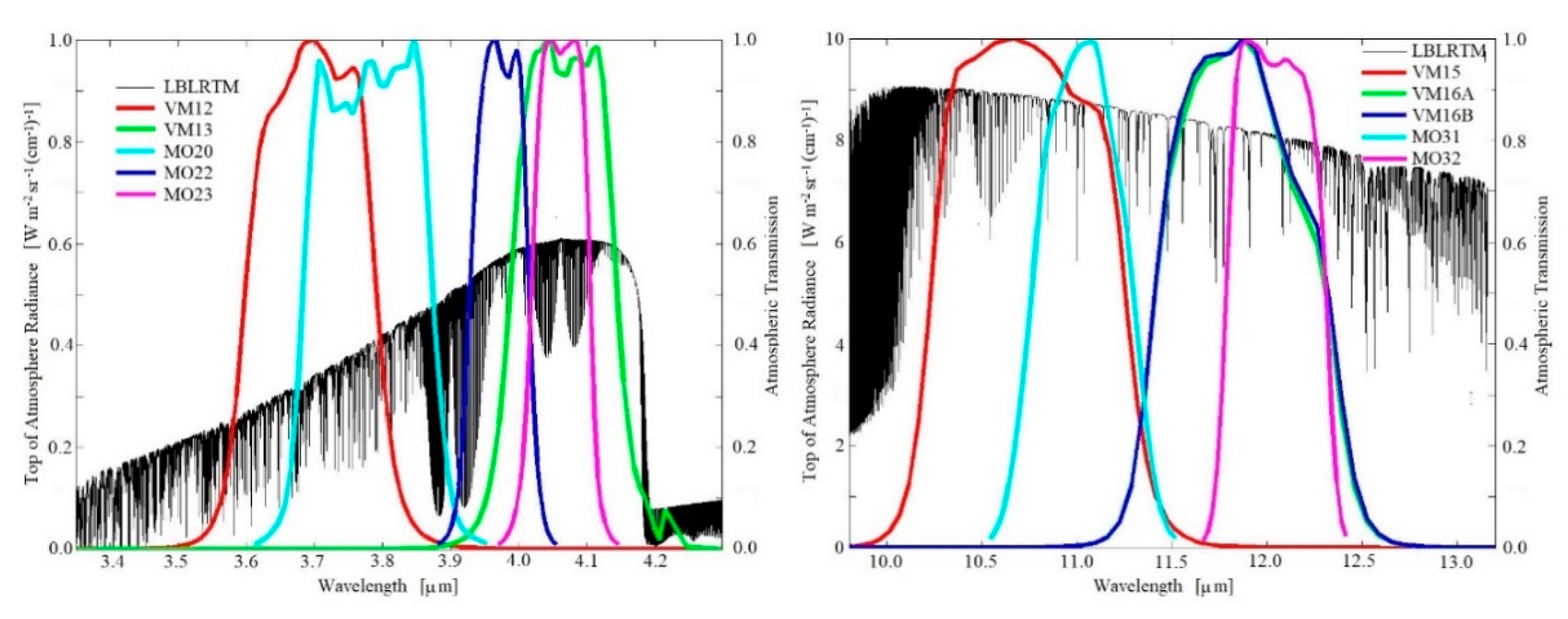
The spectral characteristics of the IR bands are constrained by the atmospheric transmission as an SST_skin retrieval requires the sensed signal to have a useful component originating at the surface, even though it is modified by the intervening atmosphere. As with the heritage instruments, the VIIRS bands used for SST_skin retrieval are placed in two atmospheric transmission “windows” in the mid-IR (3.5 μm < λ < 4.1 μm) and in the thermal IR (10 μm < λ < 13 μm). In Figure 1, the atmospheric transmission spectrum was calculated using the Line-By-Line Radiative Transfer Model (LBLRTM) [51] with the atmospheric profiles of temperature and humidity taken from ECMWF ERA-Interim [52] reanalysis dataset for 1 July 2009 at 00:00 at 00.0° N, 00.0° E. Other gases were taken from the Standard Tropical Atmosphere. The spectroscopic properties of the gases were taken from the HITRAN database [53]. The VIIRS bandwidths, being about 1 μm, are more comparable to those of the AVHRR, and are about twice as wide as the corresponding MODIS bands (Figure 1;

Table 1. Spectral characteristics of MODIS and VIIRS IR bands designed to be used for the retrieval of SST_skin. Bandwidth is given as full width half maximum positions. The Noise Equivalent Temperature Differences (NEδT) are specified for a typical scene temperature: 300 K for all bands except for VIIRS M13, which is 270 K. After [49,56].

MODIS			VIIRS
Band	Spectral Bandpass μm	Specified NEδT K	Band	Spectral Bandpass μm	Specified NEδT K
20	3.660–3.840	0.05	M12	3.610–3.790	0.13
22	3.929–3.989	0.07
23	4.020–4.080	0.07	M13	3.973–4.128	0.18
31	10.780–11.280	0.05	M15	10.263–11.263	0.07
32	11.770–12.270	0.05	M16	11.538–12.488	0.07

). The specified Noise Equivalent Temperature Differences (NEδT) have been found to be smaller on orbit for both MODISs on Terra and Aqua [54] than for S-NPP VIIRS [55]. Small NEδT is desirable as it means that each brightness temperature derived from the radiance measurement is less noisy, and that the brightness temperature differences needed in the atmospheric correction algorithm (see Section 4.2) are also more accurate, and become dominated by noise at smaller values.

The range of rotating telescope angles for which earth view data are taken is ±56° from nadir, resulting in a swath width of ~3000 km, which is wide enough to ensure overlap of adjacent swaths at all latitudes.

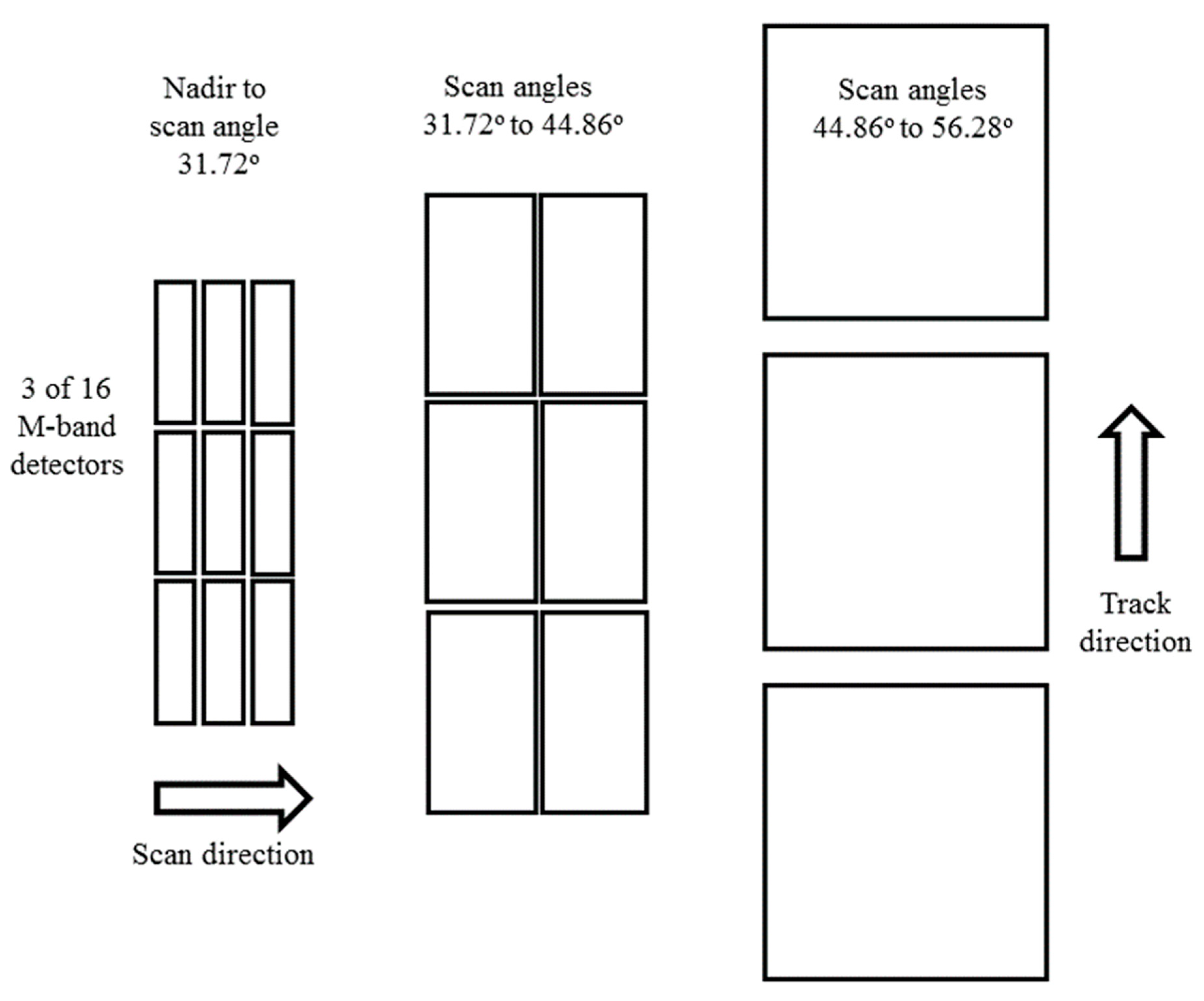
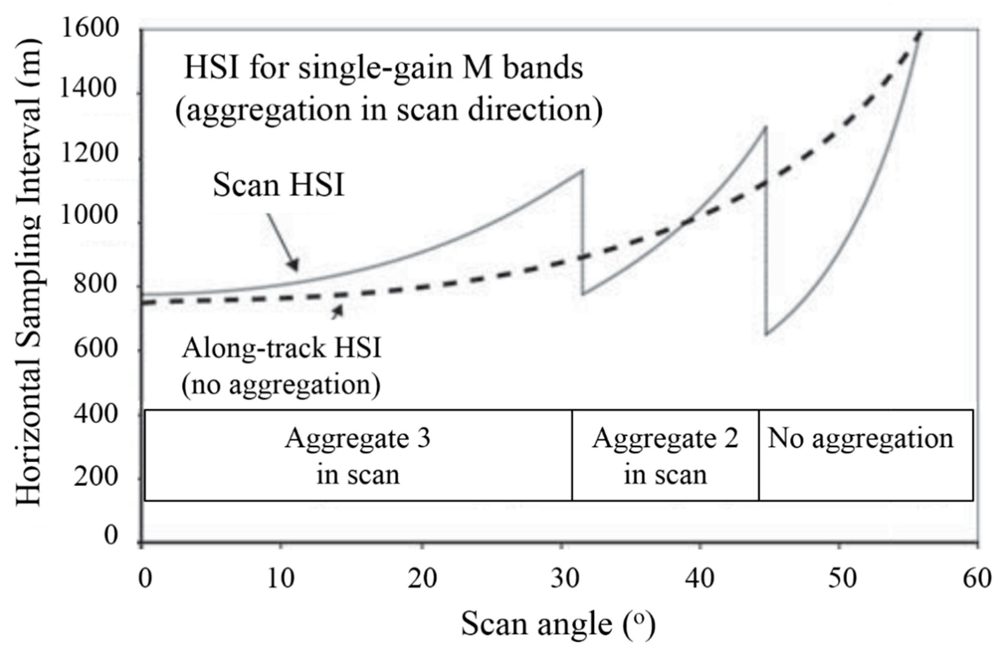
A new feature of the VIIRS optical system and on-orbit processing is pixel aggregation. This approach was developed to reduce the growth in pixel size that results from the earth’s curvature and beam spreading along longer atmospheric paths away from nadir, often referred to as the “bow-tie” effect. The native nadir pixel size for the moderate resolution bands, which include those used for SST_skin retrievals, is ~250 m in the scan direction and ~750 m in the along-track direction. Three successive measurements are averaged on-board prior to transmission to ground to yield the pixel size of 750 × 750 m² at nadir. At absolute scan angles >31.72° from nadir, the on-board processor averages two successive measurements. Finally, for absolute scan angles >47.87° individual measurements are transmitted (Figure 2) [48,57,58]. At each aggregation transition, the horizontal sampling interval along the swath returns a value close to that at nadir. This results in much smaller growth in the size of the samples towards the edges of the swath (Figure 3) and this is much less for VIIRS than for previous broad swath imaging radiometers.

3. Independent Validation Data

Our approach to assessing the scientific quality of the VIIRS SST_skin retrievals is based on comparisons with SSTs from other sources. Comparisons with other global SST fields were made early in the VIIRS mission to assess the overall credibility of the derived SST_skin. However, such comparisons are sometimes difficult to interpret in a quantitative fashion as the fields being used as a reference have their own issues; the spatial distributions of their errors and uncertainties are generally not well known, other than similar inaccuracies will occur in similar conditions. For quantitative comparisons we use independent subsurface temperature measurements from buoys, drifting and moored, and SST_skin from ship-based radiometers. In this section, we describe the results of quantitative assessments of VIIRS SST_skin retrievals, but first we introduce other relevant SST fields used during VIIRS algorithm development and testing.

3.1. Global Satellite-Derived Reference Fields

For the earlier processing algorithms (NASA VIIRS R2016.0 and R2016.1), Daily Optimally Interpolated SST fields (DOISST) downloaded from the National Center for Environmental Information (NOAA/NCEI) archive were used as a reference field. These DOISST fields were compared with the VIIRS retrievals to identify rogue values that may result from undetected sources, such as cloudy pixels being misidentified as clear sky, or unknown instrumental artifacts. The DOISST are interpolated 0.25° gridded fields derived from AVHRR Pathfinder V5 SSTs [18] and SSTs from buoys and ships to produce gap-free fields [59,60,61]. The DOISST is frequently referred to as the “Reynolds” SST fields (v1: [62]; v2: [59]). The DOISST fields are bias corrected to represent a subsurface temperature without diurnal warming; for drifting buoys, the temperature is typically measured at a depth of ~20 cm. As discussed in Section 1, the sub-surface temperature represented in the DOISST fields is typically warmer than the cool skin temperature measured through the emission depth of the IR radiation. For comparisons to the SST_skin in this study, the DOISST was adjusted to a colder skin temperature by adding −0.17 K, which is an estimate of the average difference under moderate and high winds between the temperatures of the skin and at the depth of the drifting buoy measurements often found over large regions of the ocean [39,40,63]. This adjustment may not always be sufficient, for example in very low wind speed conditions. In the daytime the effect of low winds is enhanced by high solar illumination, leading to a variable relationship between SST_skin and subsurface temperature, e.g., [64].

For the recently reprocessed NASA VIIRS SST products, referred to as R2016.2, the SST reference fields were changed to those of the Canadian Meteorological Center Global Foundation Sea Surface Temperature (CMCSST) [65] due to degradation and calibration issues of several of the more recent AVHRR sensors and the progressive loss of a significant number of in situ observations used in the DOISST interpolation [66].

3.2. SST Fields from Microwave Radiometers

Comparisons are presented below between VIIRS SST_skin and SSTs derived from sensors operating in the microwave range of the electromagnetic spectrum, which are generally insensitive to the presence of most clouds. Instead, coverage gaps in the swaths result primarily from heavy rainfall [67], but some are also from high winds, >20 m s⁻¹, sun glint, and radio frequency interference [68,69]. Furthermore, microwave SST retrievals are not feasible within about 75 km of the coast and sea ice edges. As in the IR, emission from the ocean surface at microwave frequencies comes from the electromagnetic skin layer on the aqueous side of the interface, but it extends several millimeters below the thermal skin layer ([70]; Ch. 8 of [30]). Thus, the microwave emission contains components from both the thermal skin layer and the water beneath, and the retrieved SST is a measure of both the sub-skin and skin layer temperatures. In an exhaustive study of comparisons between WindSat (see below) SST retrievals and measurements from drifting buoys, Gentemann [71] found mean differences of −0.05 ± 0.55 K for descending arcs (06:00 Equator crossing time) and 0.02 ± 0.52 K for ascending arcs (18:00 Equator crossing time). Similarly, for AMSR2, Gentemann and Hilburn [69] found mean differences of −0.02 ± 0.55 K for descending arcs (01:30 Equator crossing time) and −0.09 ± 0.55 K for ascending arcs (13:30 Equator crossing time). The mean difference of all of these comparisons, 862,729 in total, is −0.015 K, rounded to −0.02 K. For comparisons with VIIRS SST_skin the microwave-derived temperature fields were adjusted to a skin temperature by adding −0.15 K. We refer to this as SST_μw, although some authors refer to passive microwave radiometer SST estimates as a sub-skin temperature (SST_sub-skin).

3.2.1. WindSat

WindSat is an 11-channel, 5-frequency satellite-borne polarimetric microwave radiometer [72] and is the main instrument on the DoD—US Navy Coriolis satellite launched on 6 January 2003. At an altitude of 840 km, Coriolis is in a sun-synchronous orbit with an ascending node time of ~18:00, and thus in a terminator, or dawn-dusk, orbit. The geometry of the conical scan measurement results in WindSat taking five days to provide almost gap-free coverage of the globe. The surface resolution of the SST retrievals is relatively coarse at 39 km × 71 km. Global, gap-free, reference fields were generated for each day by aggregating five days of WindSat data, separately for night and day observations, centered on the middle day.

3.2.2. AMSR2

The Advanced Microwave Scanning Radiometer 2 (AMSR2) was launched on 18 May 2012 on the Japanese Shizuku satellite, also called GCOM-W1 (Global Change Observation Mission—Water Satellite 1) and is part of the A-Train. The AMSR2 antenna, 2 m diameter, is larger than those of earlier earth observation microwave radiometers and thus has a smaller footprint at the sea surface, 35 km × 46 km at the low-frequency channels used for SST retrievals. AMSR2 measurements cover >99% of the earth’s surface every two days.

3.3. Drifting and Moored Buoys

Quality-controlled subsurface in situ temperatures from drifting and moored buoys were used to generate matchups with the satellite data, which require the surface data to be within 30 min and 10 km of the center of the satellite pixel [73]. The quality assurance is performed by the NOAA iQuam (in situ Quality Monitor [74]), which is interrogated on a daily basis for the matchup generation. An example of the distribution of the VIIRS-buoy matchups is shown in Figure 4. It has become apparent that the accuracies of the thermometers in the drifting buoys are poorer than the ~0.1 K that was assumed earlier, and probably are closer to ~0.25 K [75,76,77]. This means that the uncertainties in the buoy measurements can make a significant contribution to the discrepancies between the satellite and in situ temperature retrievals.

3.4. Shipboard Radiometers—M-AERI

SST_skin values for VIIRS validation have been taken by Marine-Atmospheric Emitted Radiance Interferometers (M-AERI) [78], which are Fourier Transform spectroradiometers that take measurements of the IR emission from the sea surface and atmosphere in the wavelength range of 3 to 18 μm. Newly developed second- and third-generation M-AERIs have been deployed since 2013 for VIIRS SST_skin validation. All M-AERI types have two internal black body cavities to provide accurate at-sea calibration, with the accuracy of which being confirmed by laboratory calibration before and after each field deployment. Data from the M-AERIs are included in the VIIRS SST Match-Up Database (see Section 4.3 below), and reserved for accuracy assessment of the VIIRS SST_skin retrievals. An example of the measurements taken by an M-AERI on a research vessel is given in Figure 5.

3.5. Shipboard Radiometers—ISAR

Another type of ship-board instrument, the Infrared Sea-surface temperature Autonomous Radiometer (ISAR) [79] also provides SST_skin for VIIRS validation. ISARs are autonomous filter radiometers with two internal blackbody calibration targets and, as with the M-AERIs, have pre- and post-deployment laboratory calibration to provide SI traceability. Data are relayed in real-time by the Iridium satellite telecommunications system. Two ISARs have been deployed on the M/V Andromeda Leader of NYK Lines, which plied between Japan and the USA; the round-trip took about two months (Figure 6). The ISARs are periodically swapped during port calls in the USA to allow refurbishment and recalibration without interrupting the time series of measurements.

An ISAR was mounted on the M/V Horizon Spirit as part of the DoE ARM (Atmospheric Radiation Measurements) program MAGIC field campaign [80,81]. Between September and December 2012, and May to September 2013, the ship sailed between Los Angeles, California, and Honolulu, Hawaii, taking two weeks for a round trip.

4. Processing Algorithms

As with any satellite IR imager being used to derive SST_skin from calibrated TOA Brightness Temperature (BT) measurements in appropriate spectral bands, there are two distinct data processing steps that need to be taken: (i) Identifying those measurements that are free from radiance from sources other than the surface and gaseous components of the atmosphere, and then (ii) correcting for the radiative effects of atmospheric gases. The first step is conventionally called “cloud screening” as the primary objective is to identify pixels that include radiance from clouds, and the second step is referred to as the “atmospheric correction”. The creation of a consistent SST_skin record with compatible error budgets from multiple infrared sensors can be facilitated if the data are processed using similar cloud identification methods, atmospheric correction algorithms, and ensuring that the stability and calibration accuracy of radiances be maintained on orbit.

Since launch, VIIRS ocean products have been generated by the NASA Ocean Biology Processing Group (OBPG), which uses the convention of identifying each reprocessed version of the satellite-derived variables with the letter “R” followed by the year in which year an algorithm or significant calibration change was introduced into production, and with decimal increments indicating minor algorithm improvements or code changes. The file metadata includes the processing code version. The current VIIRS SST_skin are designated R2016.2.

4.1. Cloud Screening

As with MODIS, for VIIRS we initially developed a recursive binary “classification-tree” to identify cloud contaminated measurements [5], based on the approach originally developed for the AVHRR Pathfinder program [18]. Generally, these Binary Decision Trees (BDTrees) are similar between day and night and are dominated by Long-Wave IR (LWIR) channel differences and spatial uniformity tests. However, in the daytime part of each orbit, reflected sunlight provides additional information allowing us to distinguish between the high reflectance clouds from the low reflectance sea surface. A factor that complicates the daytime decision tree is the high surface reflectance that occurs in regions of sun glitter; a separate set of tests is needed for these conditions. The differences in performance metrics, such as sensitivity and specificity [82] of the decision-trees between day, night, and sun-glitter conditions, were expected to lead to differences in the effectiveness in the identification of cloud-free conditions. Research on sampling errors in derived SST_skin resulting from the presence of clouds however revealed significant differences in cloud persistence between day and night [83,84]. These findings are difficult to explain by physical processes, suggesting a problem with the cloud-screening algorithms in certain conditions, and so prompted a reassessment of the performance of the cloud screening approach. The false cloud-induced sampling errors were most severe at moderate to high latitudes in both hemispheres particularly in the daytime, and were initially identified in MODIS data, but subsequently also found in the early preliminary VIIRS fields.

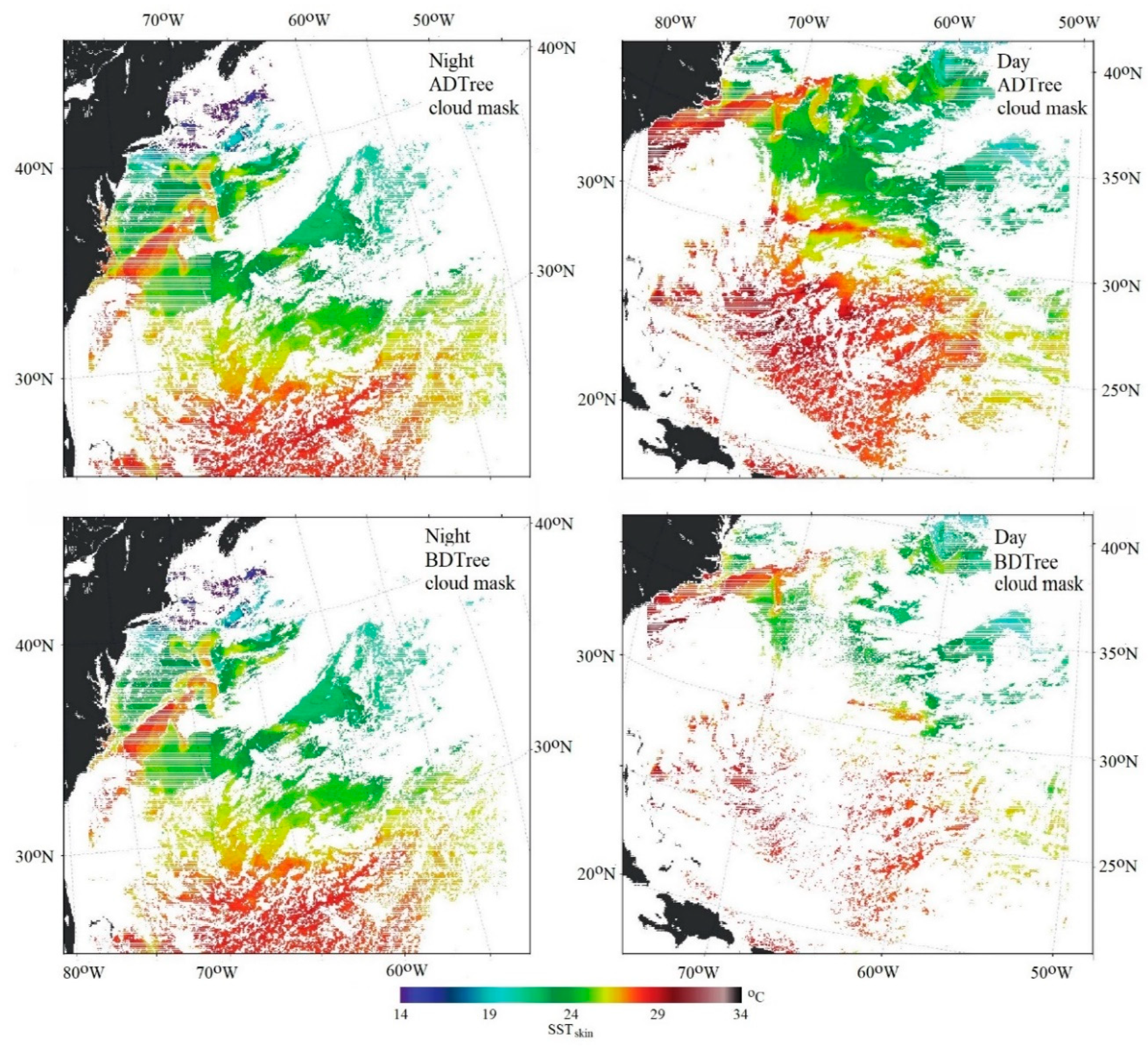
The revised cloud screening algorithm for R2016.0 and subsequent versions of the VIIRS SST_skin retrievals is based on the machine learning approach of Alternating Decision Trees (ADTrees) [85,86]. The ADTree algorithm involves a collection of binary decision nodes forming a “branch” ending with a prediction node. Nodes contain a “vote” that is scaled to the predictive power of the test. When combined with “boosting algorithms”, where at each training iteration instances that were previously misclassified are given a larger weight, an accurate ensemble classification model can be developed. To predict likely cloud contamination, a pixel transits all decision nodes that are true, and the prediction values from all true nodes are summed to form the final vote. For VIIRS data, a positive sum indicates clear skies and a negative vote is cloudy. The magnitude of the vote provides an indication of the confidence in the classification for a given pixel. In some instances, the combined vote from a collection of weak prediction nodes when voting in the same way can modify or override the vote of a single strong prediction node. This new approach was developed for four classes of conditions: (i) Nighttime, (ii) daytime with glint coefficient ≤ 0.005, (iii) daytime moderate glint coefficient between 0.005 to 0.01, and (iv) daytime severe glint when 678 nm red reflectance >0.065. The use of the new classification algorithm improves the coverage of the VIIRS data in daily global maps by about ~5–10% at night and up to 60% during daytime depending on the location and season, indicating significant false positives (clear pixels flagged as cloudy) in the previous cloud-screening algorithms. The ADTree approach also improves the discrimination of clouds near ocean thermal fronts that were frequently misclassified as cloudy as a result of the large horizontal SST_skin gradients. Example VIIRS images using the ADTree classifier show improved retention of good quality pixels compared to the BDTree cloud screening are shown in Figure 7. The ADTree approach is described in greater detail by Kilpatrick et al. [16].

4.2. Atmospheric Correction Algorithms

The heritage sensor for SST_skin from VIIRS is MODIS, with VIIRS having four of the five bands that MODIS uses for retrieving SST_skin (Table 1). Because of the influence of reflected and scattered solar radiation, measurements of satellite radiometers taken in the mid-infrared atmospheric transmission window cannot be used in the daytime portion of the orbit. As a result, NASA produces three distinct SST_skin products for VIIRS, as for MODIS. A pair of standard day and night retrievals, referred to as SST_skin, provide continuity and consistency with the 30+ year record of measurements from AVHHR [18] and MODIS [5]. The pair of standard products also facilitate the study of diurnal heating as the algorithm and coefficients are applied consistently between day and night. The second night-only product, SST_triple, is produced to take advantage of the cleaner atmospheric transmission window in the mid-infrared bands (MWIR) on both VIIRS and MODIS, capable of producing retrievals with lower uncertainty.

The atmospheric correction used for the standard SST_skin retrieval is based on measurements in the 10–13 μm atmospheric transmission window, often referred to as a “split-window” algorithm and is derived from the same algorithm form used for both MODIS and AVHRR Pathfinder—the Non-Linear SST (NLSST) [87]:

SST_skin = a₀ + a₁T₁₁ +a₂(T₁₁ − T₁₂) T_sfc + a₃ (T₁₁ − T₁₂) (sec(θ) − 1)

(1)

where SST_skin is the SST_skin derived during the day or night; a₀, …, a₃ are coefficients, T₁₁ is the BT measured in the band centered near λ = 11 µm (VIIRS band M15), T₁₂ is the BT measured in the band centered near λ = 12 µm (VIIRS band M16). T_sfc is a first guess or climatological SST that scales the coefficient, multiplying the T₁₁–T₁₂ BT difference to account primarily for the effects of atmospheric water vapor (see Figure 5 of Minnett et al. [12]), the main cause of the atmospheric effect in these infrared spectral intervals [87], and which is correlated with the SST [88]. The unit of T_sfc is °C with a lower bound of zero to prevent the difference term from becoming negative. θ is the satellite zenith angle and this term compensates for the increasing atmospheric path length when the view angle is off-nadir. The coefficients in this equation and those below have been derived through regression analyses of the TOA BTs in the relevant VIIRS bands in conditions that have been identified as cloud-free, with coincident and contemporaneous in situ measurements from drifting and moored buoys and ancillary variables θ and T_sfc.

Building on our experience with both MODISs, the VIIRS R2016.0 algorithms use month-of-year coefficients estimated separately for six latitude bands (with boundaries at the Equator, ±20° and ±40°), thus there are 72 sets of coefficients. Coefficients are estimated from randomly selected 65% of the matchups identified as suitable for this purpose by the cloud decision trees and other quality tests (see Section 4.4 and Appendix A); the remaining 35% of the matchups is withheld to determine uncertainties. Tapered weights are applied within 5° of latitude of the boundaries of the latitudinal bands to avoid unphysical abrupt transitions in the atmospheric correction when transitioning from one latitude band to the other. These geographical coefficients provide a better seasonal atmospheric correction for both hemispheres independently compared to earlier approaches applied to MODIS measurements, which assumed the seasonality and geographic variability in the atmosphere could be captured by the 11–12 μm BT difference alone [5].

The mid-IR MODIS nighttime algorithm is based on measurements in very narrow spectral bands at λ = 3.95 μm and 4.05 μm, but this pair is missing from VIIRS. Therefore, an algorithm similar to Equation (1) for application to nighttime measurements including the VIIRS band at λ = 3.7 μm (M12) is used. The resulting retrieval for this second nighttime SST_skin is referred to here as SST_triple and is based on the NLSST triple window SST algorithm [87]:

SST_triple = a₀ + a₁ T₁₁ + a₂ (T_3.7 − T₁₂) T_sfc + a₃ (sec(θ) − 1)

(2)

At ~3000 km, the swath of VIIRS is wider than the 2440 km swath of MODIS, which results in there being no gaps on the ocean surface between adjacent swaths of successive ascending or descending arcs. To facilitate accurate SST retrieval across the entire swath, additional terms have been added to the MODIS and VIIRS atmospheric correction algorithms to account for the effects at the high emission angles and long atmospheric path lengths:

SST_skin = a₀ + a₁T₁₁ +a₂(T₁₁ − T₁₂) T_sfc + a₃ (T₁₁ − T₁₂) (sec(θ) − 1) + a₄ (θ) + a₅ (θ²)

(3)

A further term has been added to the MODIS version of Equation (3) to take into account small differences in the reflectivity of the two sides of the mirror, but that is not required for VIIRS. For the nighttime retrievals:

SST_triple = a₀ + a₁ T₁₁ +a₂ (T_3.7 − T₁₂) T_sfc + a₃ (sec(θ) − 1) + a₄ (θ) + a₅ (θ²)

(4)

Equations (3) and (4) together form the VIIRS R2016.0 and subsequent atmospheric correction algorithms. The VIIRS R2016.2 algorithms differ from earlier versions by the use of CMCSST reference fields instead of the DOISSTs, as T_sfc for daytime SST_skin and SST_triple. At night T_sfc is the SST_triple if available, otherwise it is the CMCSST value.

Coefficients for the algorithms are available at https://oceancolor.gsfc.nasa.gov/atbd/sst/viirs-npp_sst_coeffcients_v6.4.1.nc and https://oceancolor.gsfc.nasa.gov/atbd/sst_triple/.

4.3. Processing Overview

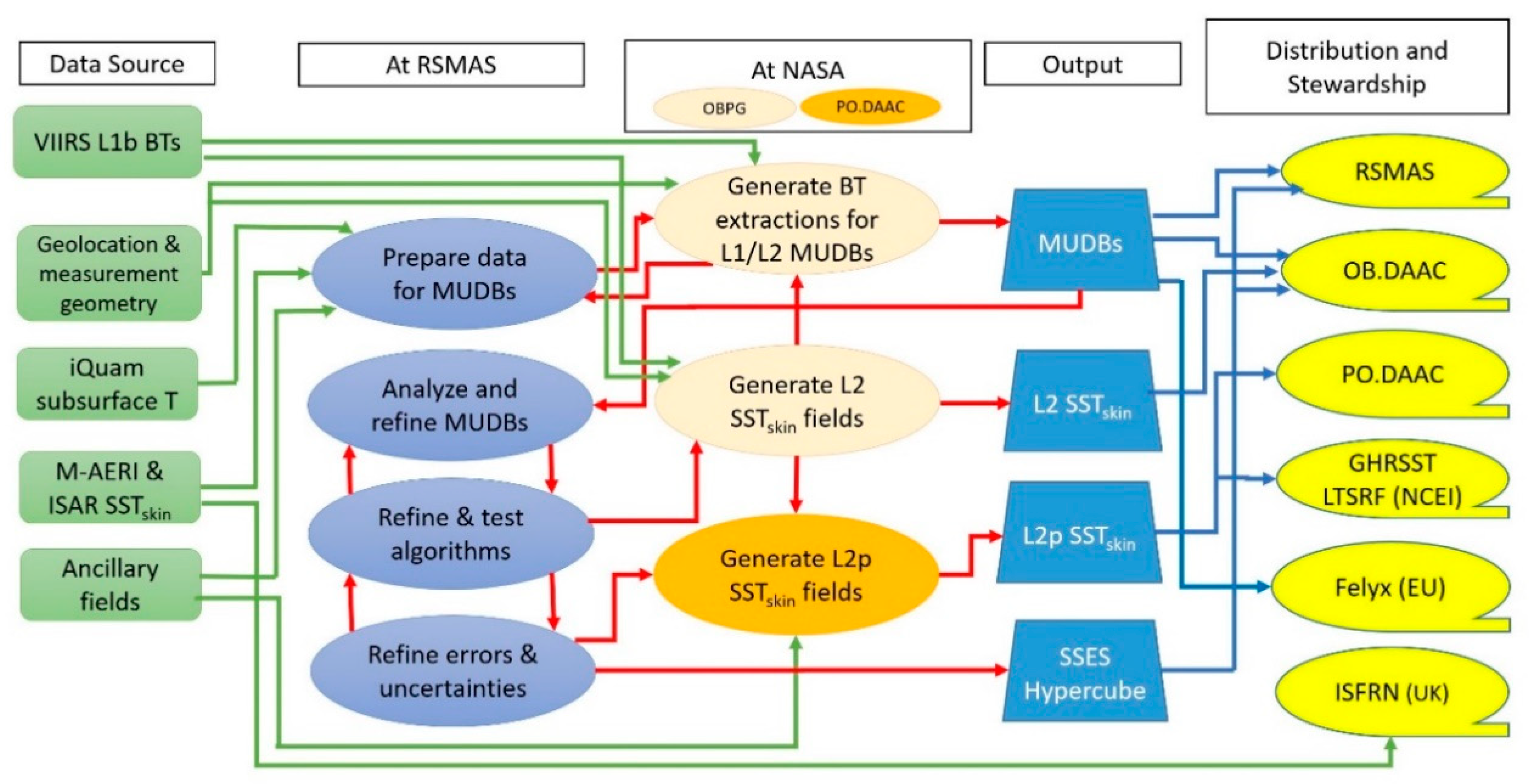
The S-NPP VIIRS SST_skin files are produced by the OBPG and distributed by the NASA Ocean Biology Distributed Active Archive Center (OB.DAAC), both located at Goddard Space Flight Center, and in GHRSST L2p format (see below) by the Physical Oceanography Distributed Active Archive Center at the Jet Propulsion Laboratory. The data flow for the derivation of VIIRS SST_skin fields is shown in Figure 8, which includes the main steps in generating matchup databases (MUDBs) that are critical to deriving algorithms applied to the VIIRS data to derive the SST_skin retrievals in near-real time, and in reprocessing the entire mission data when significant benefit is to be gained.

The NASA processing levels are defined by Parkinson, et al. [89] and summarized in

Table 2. NASA definitions of processing levels.

Level 0	Reconstructed, unprocessed instrument/payload data at full resolution; any and all communications artifacts, e.g., synchronization frames, communications headers, duplicate data removed.
Level 1A	Reconstructed, unprocessed instrument data at full resolution, time-referenced, and annotated with ancillary information, including radiometric and geometric calibration coefficients and geo-referencing parameters, e.g., satellite ephemeris, computed and appended but not applied to the Level 0 data.
Level 1B	Level 1A data that have been processed to sensor units.
Level 2	Derived geophysical variables at the same resolution and location as the Level 1 source data.
Level 3	Variables mapped on uniform space-time grids, usually with some completeness and consistency.
Level 4	Model output or results from analyses of lower level data, e.g., variables derived from multiple measurements.

.

Within GHRSST, several subdivisions of the L2 and L3 designations were developed, and of most interest here is the L2p, meaning “L2 preprocessed” level [90]. L2p files comprise the same SST values in the same geographical coordinates as the parent L2 file, with estimates of pixel-by-pixel mean error and standard deviation error often derived from the MUDBs of in situ and satellite data, with ancillary data that may include surface wind speed, aerosol optical depth, sea ice concentration, time of measurement, and a set of quality control flags. The additional information is intended to guide the users in the application of the SST retrievals in a meaningful way.

The Level-1 calibrated BTs are included in the MUDBs along with geolocation data, surface temperature measurements, and VIIRS SST_skin retrievals at the University of Miami’s Rosenstiel School (RSMAS) and at the Cooperative Institute for Climate and Satellites—North Carolina (CICS-NC), where prototyping of the algorithms was done. The MUDBs were used to develop the VIIRS R2016.0 cloud-screening and atmospheric correction algorithms, which were subsequently delivered to NASA OBPG, tested, and installed in their production environment. Analysis of the MUDBs provide estimates of the accuracies of the SST_skin retrievals. The MUDBs are available from the OB.DAAC through https://seabass.gsfc.nasa.gov/search/sst.

4.4. Quality Flags

A group of 15 quality flags, discussed in Appendix A, are defined for each pixel, and combined to define the final pixel quality level. Quality levels also are used to control the Level-3 binning process, as only the highest quality level values available are summed into the Level-3 geographical bin in the Integerized Sinusoidal Equal Area Grid (ISEAG) used for all NASA ocean and some other products. Users should note that the NASA L2 SST products are distributed via two different data archive systems, the OB.DAAC and Physical Oceanography Distributed Active Archive Center (PO.DAAC). The two centers use an opposite convention to identify the best quality pixels. The GSFC OBPG is the producer of the L2 SST_skin fields and uses a convention where the best quality retrievals are assigned a quality level of 0. Here we use the OBPG quality order convention. The JPL PO.DAAC primarily services the physical science and modelling communities and converts the OBPG L2 files into L2p files following the requirements of the GHRSST (Group for High-Resolution SST) [28] Data Specification 2.0. (GDS) [91] where the best quality is represented by quality level 5. The corresponding meaning of each quality level for data obtained from each center is shown in

Table 3. Quality level definitions and conventions used by different archive centers. Here we use the Ocean Biology Processing Group (OBPG) convention in all discussions.

Quality Level NASA OB.DAAC L2 Standard Format	Quality Level NASA PO.DAAC L2p GHRSST GDS2.0 Format	Meaning
0	5	Best; scan angles < 55°
1	4	Good/acceptable; in glint or high scan angle
2	3	Suspect
3	2	Bad; cloud/ice/or atmospheric correction failed
4	0	Not processed or land

.

5. Assessment of Accuracy of VIIRS SST_skin

Our approach to assessing the performance of VIIRS in producing accurate SST_skin has relied on a series of analyses:

(a) Assessing the spatial characteristics of the VIIRS SST_skin fields by comparison with global SSTs derived from other satellite sensors or as represented in analysis fields for which we have some expectation of their accuracy.

(b) Assessing the accuracies of the VIIRS SST_skin retrievals in conditions that have passed a series of cloud screening tests and other quality tests by comparing the VIIRS SST_skin at the level of individual pixels, or small arrays of adjacent pixels, with the subsurface measurements from drifting or moored buoys, i.e., using the MUDB.

(c) Assessing the accuracies of the VIIRS SST_skin retrievals, as in (b) but using ship-based infrared radiometers (M-AERIs and ISARs), which measure the infrared emission from the ocean and atmosphere leading to a direct comparison of SST_skin. As discussed above, these instruments have SI-traceable calibration to standards at the National Institute of Standards and Technology (NIST) [8] and the National Physical Laboratory (NPL) [9] and therefore are the basis of the generation of CDRs of SST [13].

5.1. Instrumental Performance and Artifacts

Because of lessons learned about the design and performance of heritage instruments, VIIRS measurements lack many of the instrumental artifacts—or at least these are much less pronounced—present, for instance, in the early data collected by MODIS on Terra. These artifacts include the “response vs. scan angle” (RVS) behavior that results from wavelength-dependent infrared reflectivity of the MODIS scan mirror varying with the angle of incidence of the radiation at the mirror surface [5,42]. With the rotating telescope of the VIIRS fore-optics, it was expected that any such effects would be caused by the double-sided half-angle-mirror; this has been quantified on orbit by Xiong et al. [55] who found it to be very small. As with MODIS, “detector banding” caused by multiple detectors in each spectral band in the along-track direction [5,92], was also found for VIIRS, but it has a much smaller magnitude [93]. While there is evidence of other instrumental artifacts, they are not a major source of qualitative or quantitative shortcomings of the infrared channels for the S-NPP VIIRS.

5.2. Calibration

Our analyses have not revealed any fundamental problems with the on-board calibration of the VIIRS infrared channels, in agreement with an earlier study of Efremova et al. [94]. Nevertheless, the impacts of such problems on derived quantities can be quite subtle and may be revealed only through analyses of longer time series of data.

5.3. Spatial Distribution of Differences with Heritage Data

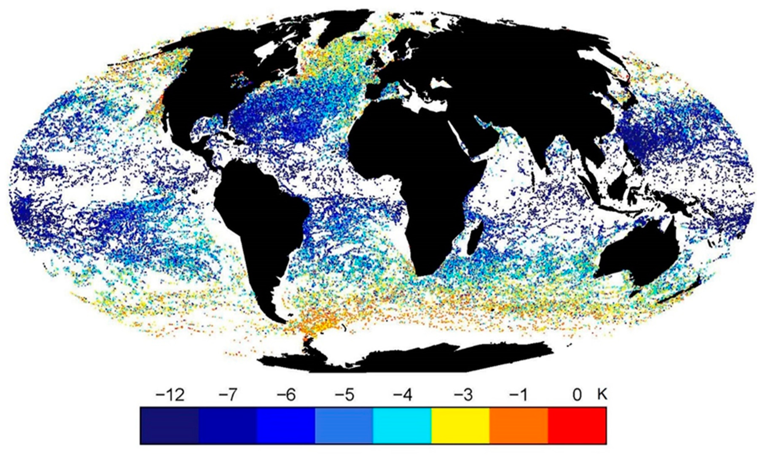
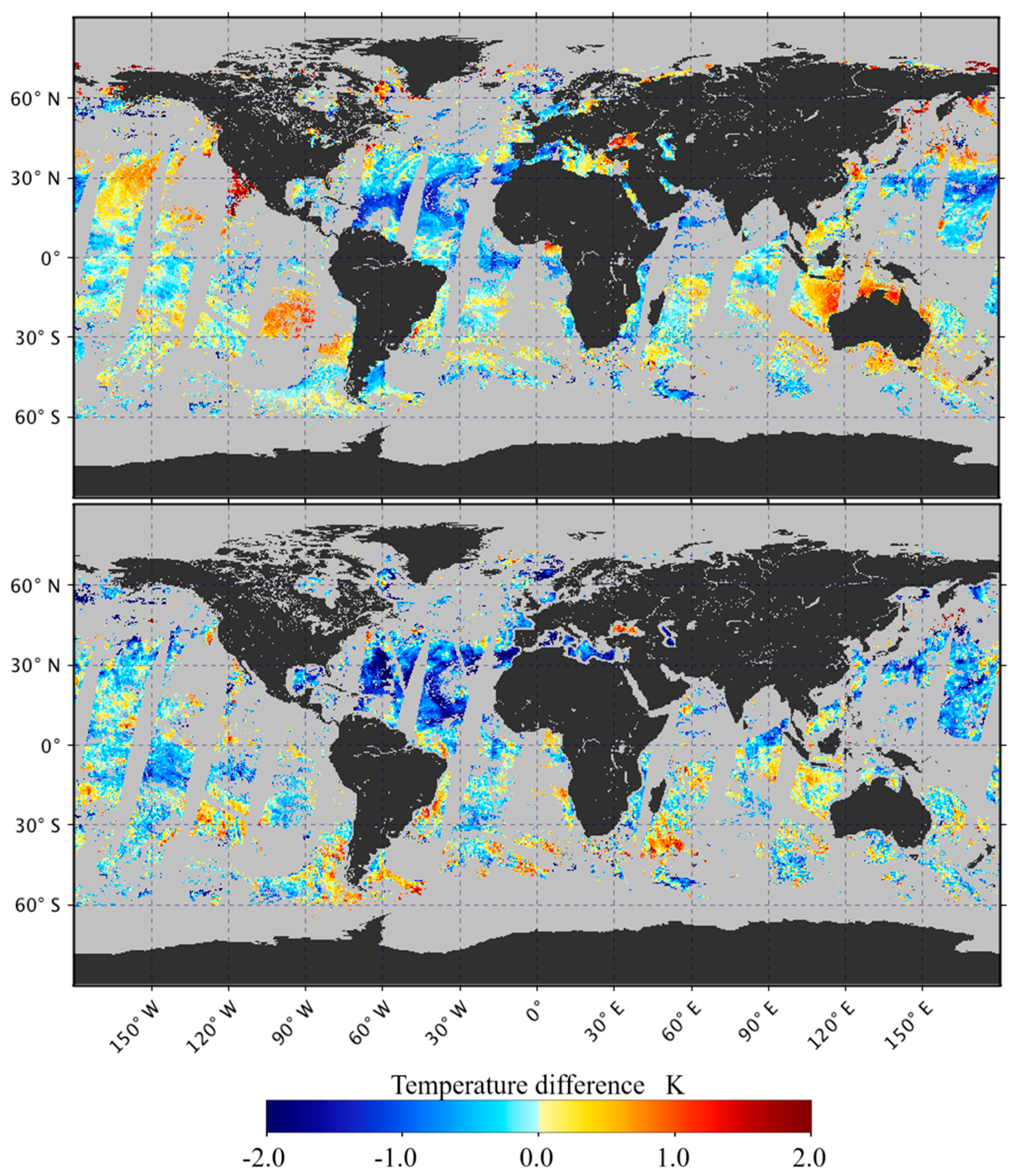
The integrity of the spatial distribution of the VIIRS SSTs has been assessed by comparisons with independent SST fields. The first reference field used was the daily, global DOISST (Section 3.2 above). An example of the difference field, VIIRS–DOISST is shown in Figure 9 (top); VIIRS SST_skin values were derived using the R2016.0 3-band nighttime algorithm (Equation (4). The data are from day 12 August 2012 and are limited to those with the best quality flag. Some blue areas indicate locations where VIIRS SST_skin retrievals are likely influenced by the presence of atmospheric aerosols, and therefore are cooler than the correct SSTs [95,96,97]. The DOISST field is tied to in situ measurements from drifting buoys for the bias correction of the AVHRR SSTs and is therefore less influenced by the atmospheric conditions. The areas where VIIRS appears to be warmer than the DOISST fields are more difficult to understand, but may be caused by the presence of dry layers [98] that can occur in the mid-level to lower troposphere [99]; however, from this comparison alone it is not clear whether the VIIRS SST_skin are showing a warm bias, or whether the DOISST have a cold bias.

Figure 9 also shows the comparison of VIIRS SST_skin with SSTs derived from the WindSat microwave radiometer. Because the sources of uncertainties in the microwave SSTs are different from those for infrared SST_skin retrievals, the uncertainties in the two fields used to derive the differences can be assumed to be uncorrelated. A concern about this comparison is that the geometry of the WindSat swaths requires compilation of five-days of measurements to generate complete global fields thus the time span between WindSat and VIIRS estimates can be over two days. Furthermore, the terminator orbit of Coriolis means the overpass times are not close to those of S-NPP, so diurnal heating and cooling may contribute to the difference; the use of nighttime VIIRS SST_skin should reduce this possible contribution. However, these concerns aside, the SSTs from WindSat are of good quality [100] and useful to assess VIIRS retrievals. The differences between VIIRS and WindSat SSTs (Figure 9, bottom) reveal the same cold bias in regions where we expect aerosol contamination of the VIIRS retrievals, off West Africa and the Arabian Sea. In contrast, the WindSat comparison lacks the areas with a warm bias when compared to the DOISST fields. Although this conclusion is not definitive, this pattern is indicative of likely regional cold biases in the DOISST fields, not warm biases in the VIIRS SST_skin retrievals.

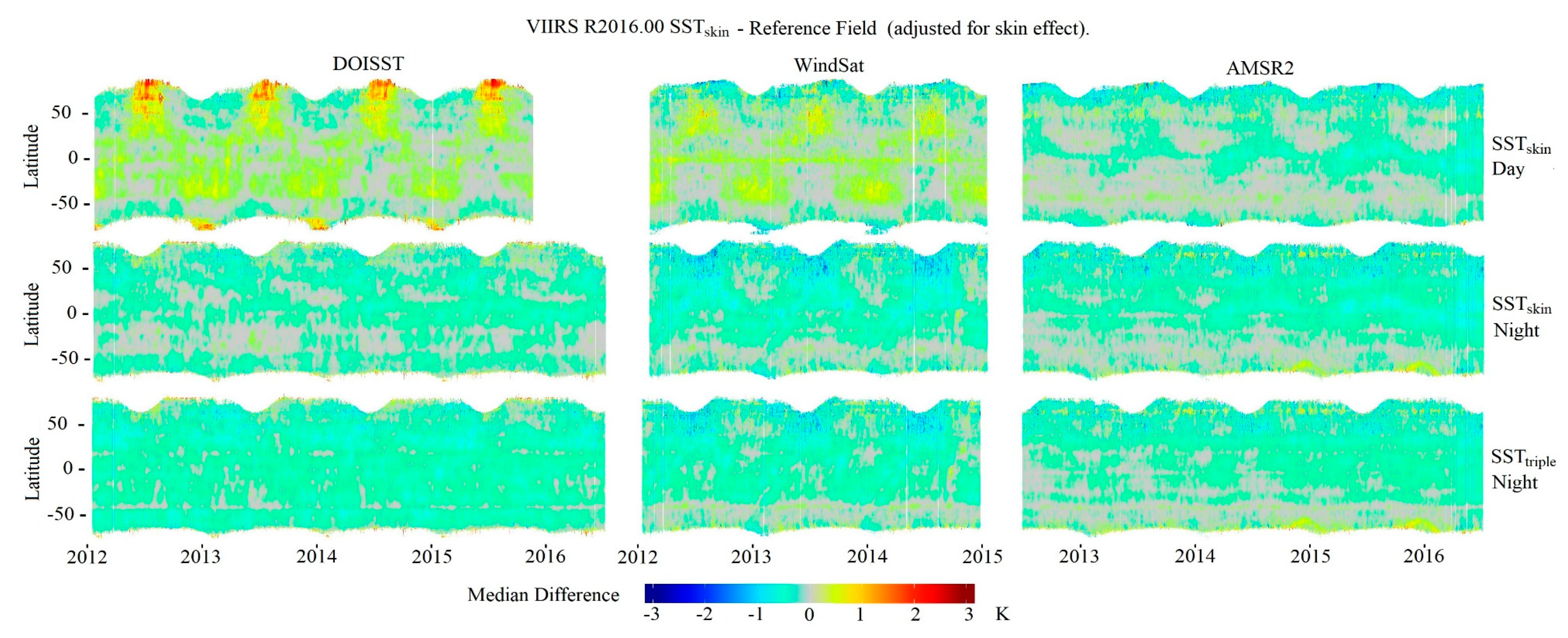
Global plots reveal the spatial pattern of the characteristics of VIIRS SST retrievals—which both reassure us and raise some concerns. However, these fields give no indication of the temporal character of retrieval behavior; Hovmöller diagrams can be used for such purpose. Figure 10 shows the daily, zonal averages of the differences between the cloud-free, best-quality (QL = 0), VIIRS R2016.0 SSTs relative to the corresponding reference fields: DOISST, WindSat, and AMSR2, SSTs. The latitudinal envelopes of the Hovmöller diagrams indicate the seasonal migration of the ice edge around Antarctica in the south, and seasonal change in solar illumination in the north.

The daytime VIIRS SST_skin derived using the two-band atmospheric correction algorithm (Equation (4)) shows a positive bias relative to DOISST of more than 2 K at high latitudes in the summer, especially in the Northern Hemisphere. This pattern of VIIRS SST_skin > DOISST has a component that is a consequence of diurnal heating of the upper ocean that is present in the daytime VIIRS SST_skin retrievals but absent from the DOISST. Also, there are some regions especially at high latitudes where the DOISST is markedly colder than temperatures measured from buoys [101]. The differences are much more uniform for both nighttime VIIRS fields with generally VIIRS SST_skin < DOISST.

Since WindSat is in a dawn-dusk orbit, diurnal heating is largely absent from WindSat fields, and this is apparent in the daytime comparison, but to a much smaller degree than for the DOISST comparison. Unlike the DOISST comparison, VIIRS SST_skin < WindSat SST_μw. at high northern latitudes during the summer, being more pronounced at night. Differences between VIIRS and WindSat SST_μw. are generally smaller in the winter in each hemisphere especially during the day; during the night, the differences are smaller in the Southern Hemisphere.

GCOM-W1, carrying AMSR2, is in the A-Train with an Equator-crossing time of 1:30 pm being the same as that of S-NPP. Although overpass times of the two satellites on a given day can differ by up to half an orbital period, ~50 min, the differences between VIIRS SST_skin and AMSR2 SST_μw. are expected to be generally small, and this is the case. During the day, the differences are smaller than for DOISST and WindSat comparisons, but with some seasonal characteristics of the AMSR2 differences. As with the WindSat comparison, VIIRS SST_skin are cooler than the microwave-derived SST_μw. at high northern latitudes, especially during summer at night, but the amplitude is smaller than for WindSat. In the Southern Hemisphere, the differences are generally much smaller. At night, VIIRS SST_skin < AMSR2 SST_μw. for most of the globe, with the exception of high southern latitudes during the summer of 2015 and 2016.

A feature that is apparent in many of the Hovmöller diagrams are zonal discrepancies that in some cases are aligned with the latitudinal band boundaries in the VIIRS atmospheric correction algorithm; this is suggestive of an issue with how the blending of the VIIRS SST_skin is accomplished at the boundaries. However, this may not be the only issue as the differences between microwave- and IR-derived SST_skin are of opposite signs for the WindSat and AMSR2 comparisons, implying that the problem cannot be isolated to the VIIRS algorithm. The nighttime zonal differences are more consistent across all comparisons at night.

5.4. Comparisons to In Situ Measurements

While the Hovmöller diagrams are useful in assessing the spatial and temporal consistencies between different satellite-derived SST_skin fields, they do not permit the attribution of the discrepancies, or parts of the differences under different circumstances, to the performance of either sensor. For this, we compare the VIIRS SST_skin to independent sea-surface, or near-surface, temperature measurements.

Global statistics of differences between R2016.0 VIIRS SST_skin and buoy temperature measurements are shown in

Table 4. Global statistics of differences between VIIRS R2016.0 SST_skin and subsurface temperatures from drifting and moored buoys. Matchup observations from October 2012 through September 2016.

	Count	Mean K	Standard Deviation K	Median K	Robust Stand. Deviation K	% Outliers
Best quality, QL = 0: satellite zenith angle < 55°
SSTskin day (Equation (3))	531140	0.200	0.534	−0.170	0.331	6.7
SSTskin night (Equation (3))	506740	−0.126	0.480	−0.129	0.340	6.5
SSTskin triple night (Equation (4))	399094	−0.145	0.349	−0.143	0.229	6.2
Good quality, QL = 1: satellite zenith angle > 55°
SST skin day (Equation (3))	251288	−0.447	0.677	−0.372	0.574	3.6
SST skin night (Equation (3))	309650	−0.324	0.736	−0.314	0.524	4.6
SST skin triple night (Equation (4))	287638	−0.247	0.499	−0.219	0.320	6.8

. The use of the median and robust standard deviation has become a more accepted method of representing the central tendency and dispersion of the differences as they are less sensitive to outliers in the distribution [5,23,102]. The negative mean and median values at night have the correct sign for the cool skin effect, [39,40,103]. Better approaches to identifying situations where large retrieval errors occur—and adjusting the algorithms or coefficient set accordingly—would improve these statistics. The accuracies of the retrievals degrade slightly when the full width of the swath is used, compared to the swath portion where the absolute satellite zenith angle is <55°.

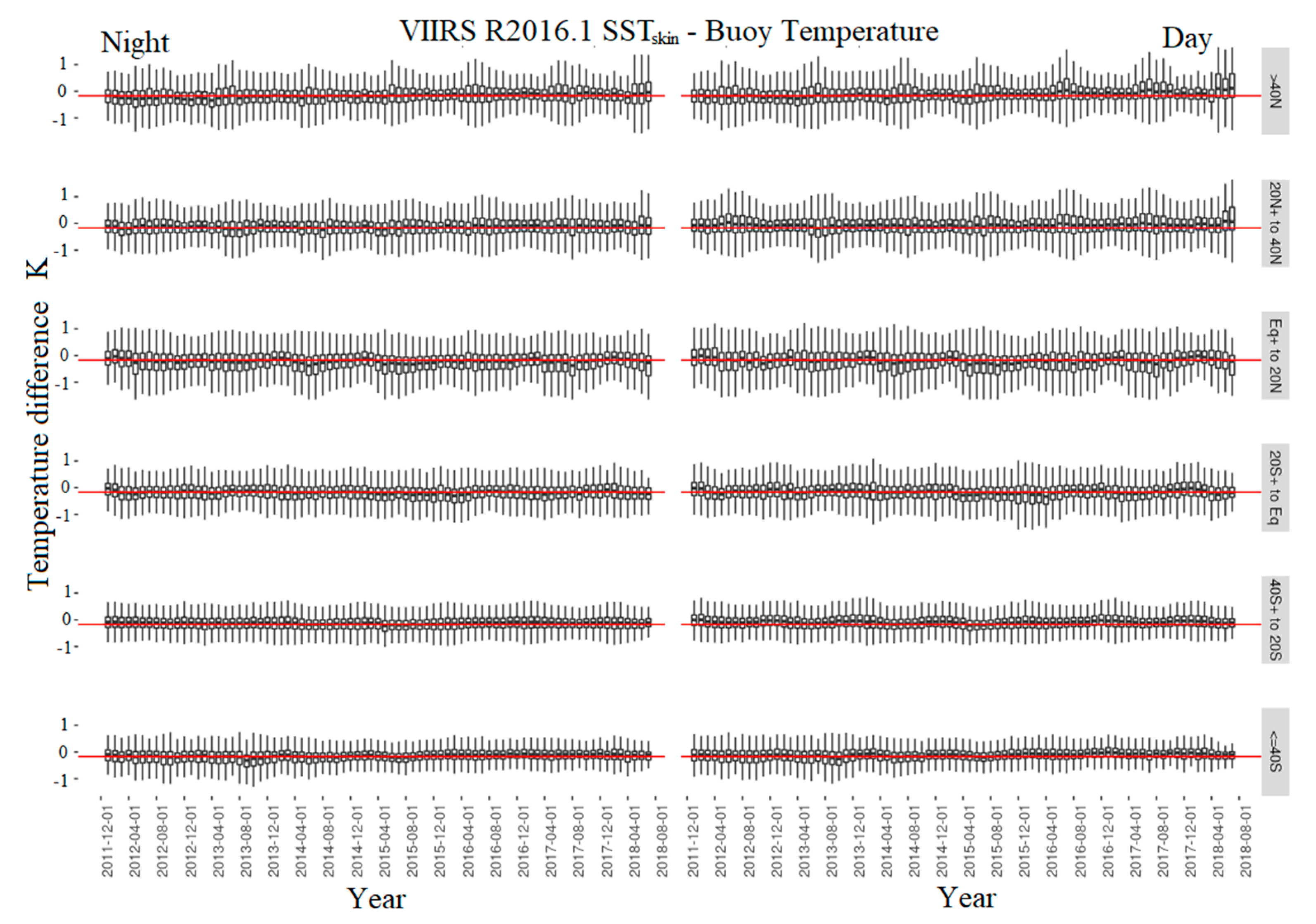
Figure 11 shows SST_skin time series of the monthly median errors in latitudinal bands, from October 2012 through August 2016. The errors and uncertainties in both the day and night SST_skin retrievals are very stable month-to-month and across latitudinal zones.

The spatial consistency of retrieval errors relative to in situ buoys corrected for the cool skin bias are shown in Figure 12 using a 5° resolution grid and best quality MUDB records for 2012–2016. Tropical regions with higher water vapor and dust aerosols indicate an increase in the robust standard deviation. Known regions with high atmospheric dust, West of Africa and in the Arabian Peninsula, generally have a cold bias often >0.5 K, indicating that the VIIRS quality flags are still not sufficiently identifying and masking episodic dust events.

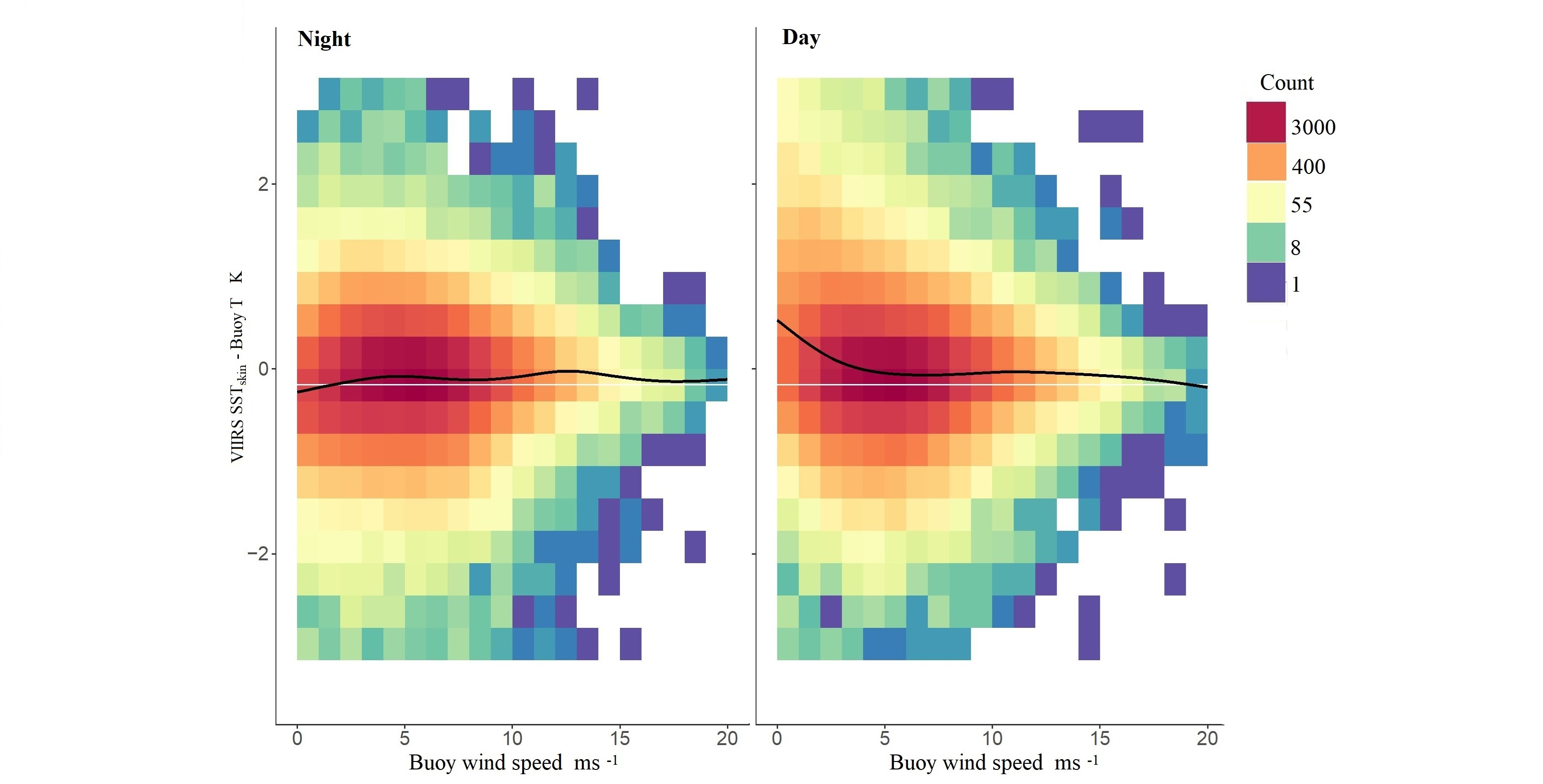
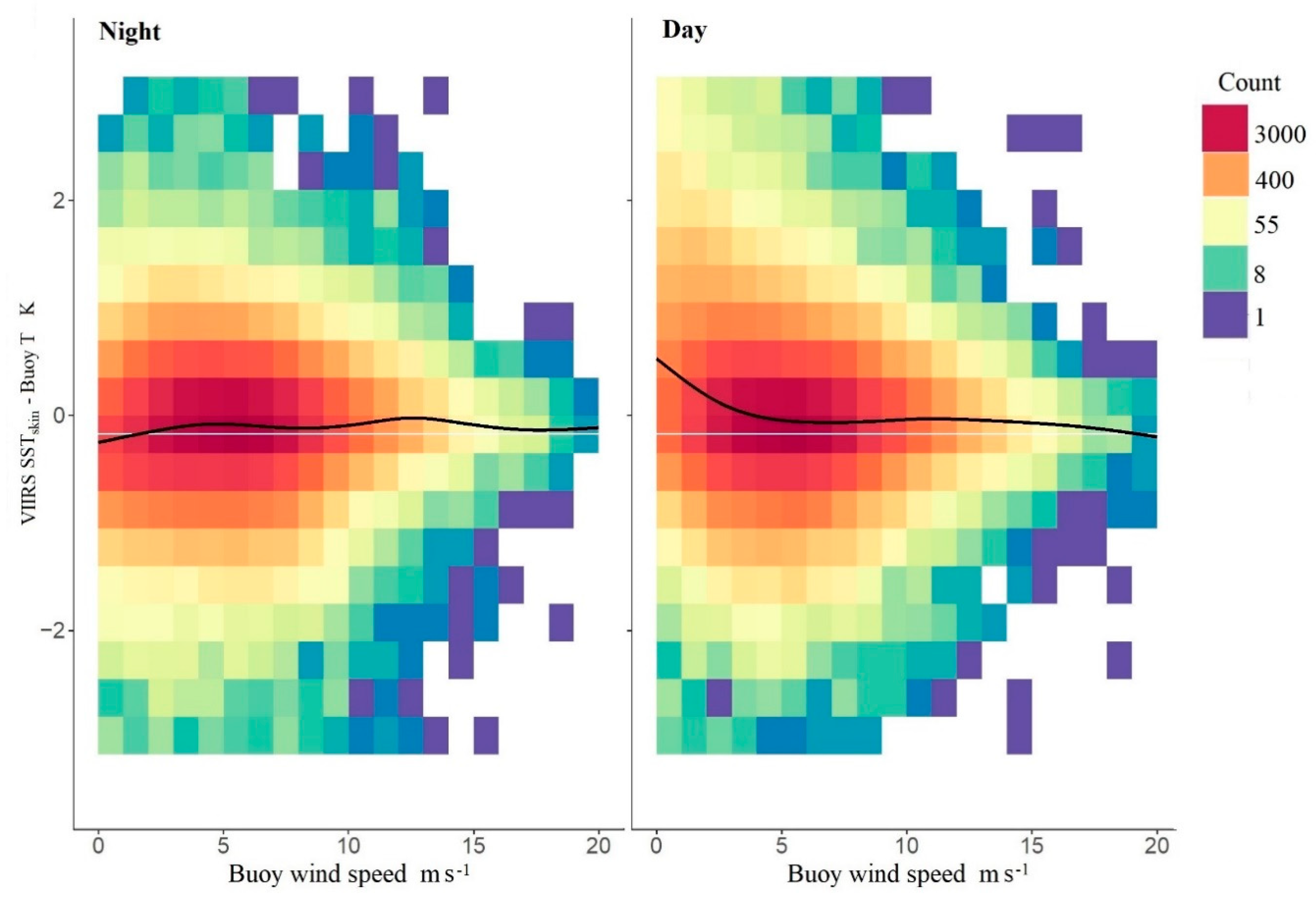
5.5. Wind Speed Dependence

There is no reason why the accuracy of the atmospheric correction algorithm for the retrieval of SSTskin from IR radiometers should be directly influenced by the wind speed in the intervening atmosphere. By wind tilting of facets of the sea surface [104], there is a potential influence through the apparent wind-speed dependence of the surface emissivity of the sea-surface [105,106,107] but this effect is very small, with the exception of high emission angles, and where the atmosphere is very dry [108]. Wind speed, however, does play a role in the comparison between VIIRS SSTskin and subsurface temperature from drifting buoys as the temperature difference between the depth of the subsurface measurement and the skin layer is wind-speed dependent. The effects of a larger temperature drop across the thermal skin layer at low winds can be seen in the nighttime distribution of VIIRS SSTskin–buoy temperature (Figure 13, left) for wind speed <2 ms⁻¹, which is in agreement with ship-based measurements [39,40]. The same effect is present in daytime conditions but is masked by the much larger positive temperature difference that results from diurnal heating (Figure 13, right).

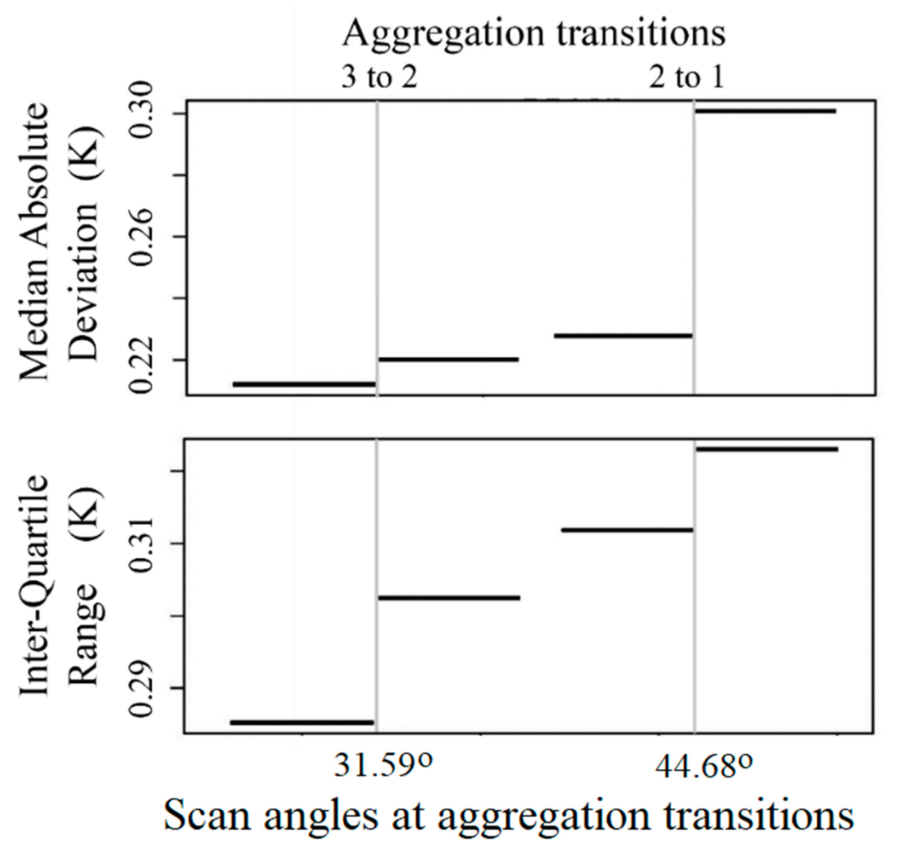
5.6. Effects of Pixel Aggregation on SST Retrievals

The VIIRS on-board pixel aggregation decreases across the scan line from 3 to 2 pixels for scan angles between 31.59° and 44.68°, and a single pixel for scan angles >44.68° (Figure 2 and Figure 3). To assess the potential impact of the varying pixel aggregation on the error budget we examined the statistics of VIIRS SST_skin relative to buoy temperatures from buoys for MUDB observations within 3 pixels on either side of the two transitions. The results (Figure 14) suggest that the aggregation scheme changes the retrieval accuracy by about ~10 mK across the swath.

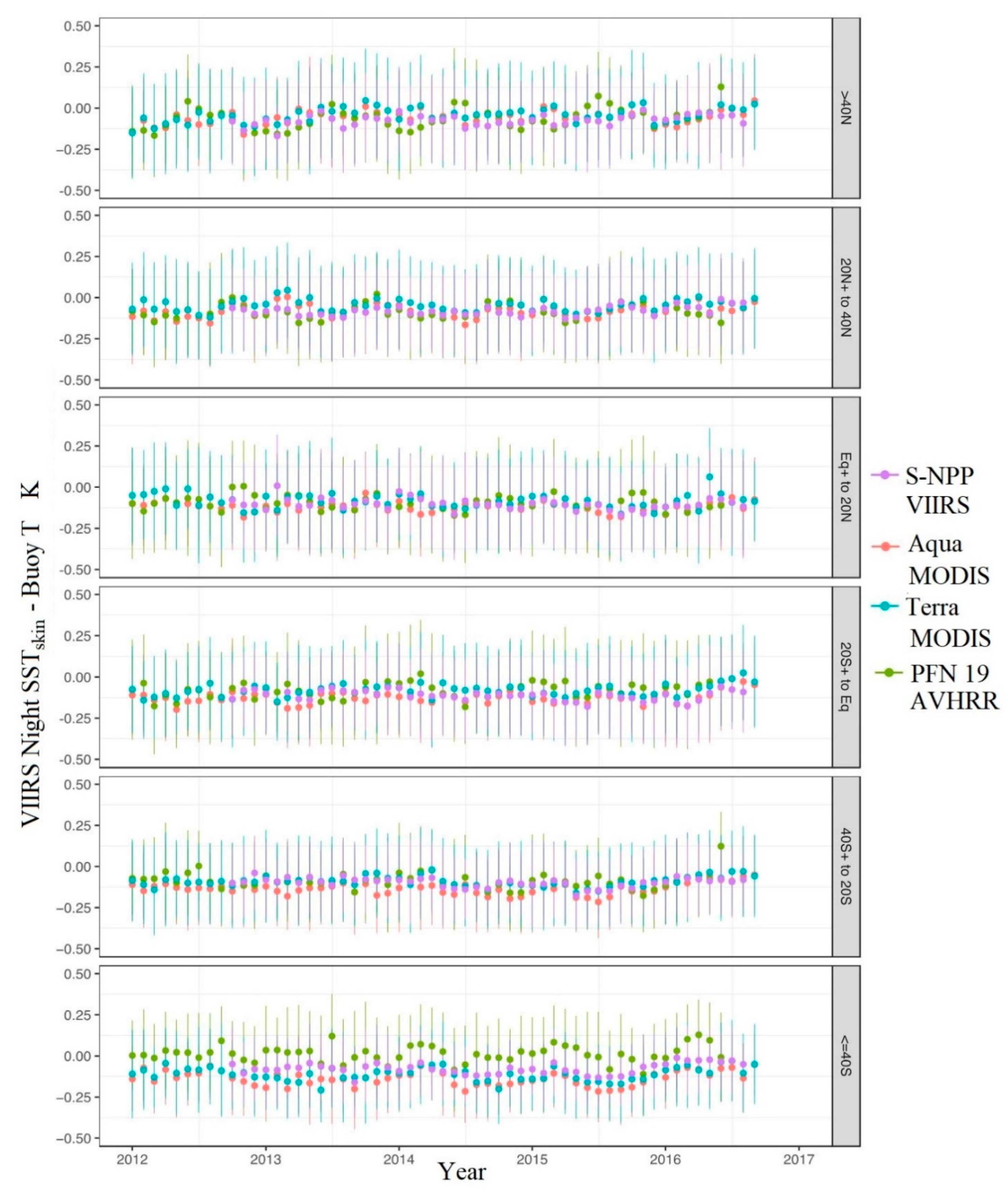
5.7. Continuity with MODIS and AVHRR SSTs

A main motivation of this study is to establish how well VIIRS SST_skin retrievals can be collated with those from other broad-swath imaging infrared satellite radiometers to generate a consistent multi-decadal series that can form the basis of an SST CDR. As discussed above, the VIIRS SST_skin processing algorithms are of the same form as those applied to the measurements of both MODISs on Terra and Aqua, and also to the AVHRR on the NOAA-19 polar-orbiting weather satellite. The time series of the global monthly medians and robust standard deviations of the differences between the satellite SST_skin retrievals and the subsurface temperature measurements show good agreement for the period starting January 2012 (Figure 15). The temperature differences are clustered around a value of −0.17 K, which is the mean skin effect. The interquartile range of the differences between the satellite SST_skin medians is 0.036 K and the robust standard deviations within each month for each satellite are in the range of 0.2–0.4 K.

The latitudinal variation in the differences between the satellite SST_skin and the subsurface temperatures also show good agreement in terms of median and robust standard deviation (Figure 15). At high southern latitudes, the AVHRR SST_skin median differences are closer to zero than those of VIIRS, and MODIS, and in mid-latitudes generally show a higher robust standard deviation.

Hovmöller diagrams of the daily differences in the zonal averages of SST_skin derived from S-NPP VIIRS and MODIS on Terra and Aqua are shown in Figure 16. The largest discrepancies are with the Terra MODIS SST_skin during the day; this is a manifestation of diurnal heating that results from the differences in the satellite overpass times. As the Equator crossing time of Terra is 10:30 compared to 13:30 for S-NPP, the VIIRS retrievals are much more likely to be influenced by diurnal heating. The diurnal heating effect is more pronounced in the Southern Hemisphere summers. In the northern hemisphere high latitudes, the overpass times of the two satellites reverse, with Terra’s being in the afternoon, and S-NPP’s being in the morning, leading to the Terra MODIS SST_skin retrievals sampling more diurnal heating than VIIRS. Also, this results in the systematic appearance each summer of VIIRS SST_skin < MODIS SST_skin for latitudes >~60° N, with smaller amplitudes at mid-latitudes. The transition from VIIRS retrievals being warmer than those of Terra MODIS to being cooler occurs in a seasonally migrating latitude. At high northern latitudes, >~60° N, in winter VIIRS SST_skin > MODIS SST_skin in a systematic pattern, which may be caused by the different band widths of the thermal IR bands of VIIRS and MODIS (Figure 1) causing the atmospheric correction algorithm to respond differently to very dry atmospheric conditions [108]. Given that Aqua and S-NPP have the same Equator crossing times, the differences in the zonally averaged SST_skin retrievals are expected to be small, and this is indeed the case with nearly all differences being <|0.2 K| and many latitudes during the day being <|0.1 K|.

The comparisons of nighttime retrievals reveal very small differences south of ~40° N for MODIS on both Terra and Aqua. North of ~40° N, the pattern is similar for both MODISs, and given the differences in the relative orbit configurations and the fact these are nighttime conditions, this pattern is unlikely to be caused by changes in the true SST_skin; instead, the differences may plausibly result from a systematic issue with the VIIRS atmospheric correction algorithm at high northern latitudes.

As with the Hovmöller diagrams of comparisons with reference fields (Figure 10), there are linear patterns at constant latitudes in all comparisons, except with Terra MODIS during the day when the signal from diurnal heating dominates. These discrepancies are at the boundaries of the latitude bands where there is a smoothed transition from SST_skin derived using one set of coefficients in the atmospheric correction algorithm to another set and are suggestive that this needs improvement.

The global statistics for nighttime VIIRS SST_skin retrievals and those of Terra and Aqua MODIS compared to subsurface temperatures from drifting buoys and M-AERIs are shown in

Table 5. Global statistics for MODIS and VIIRS night SST_skin continuity products (Equation (4)) relative to both sub-surface buoy temperatures and SST_skin derived from M-AERIs.

Sensor	Quality Level	Mean	Median	Standard Deviation	Robust Standard Deviation	Count
Sensor Night SSTskin—sub-surface buoy temperatures
Terra MODIS	0	−0.166	−0.150	0.442	0.319	538,918
Aqua MODIS	0	−0.185	−0.170	0.423	0.305	508,950
S-NPP VIIRS	0	−0.126	−0.129	0.480	0.340	506,740
Terra MODIS	1	−0.424	−0.395	0.641	0.462	252,809
Aqua MODIS	1	−0.424	−0.380	0.620	0.447	267,214
S-NPP VIIRS	1	−0.324	−0.314	0.736	0.524	251,288
Sensor Night SSTskin—SSTskin from M-AERI
Terra MODIS	0	−0.058	−0.052	0.481	0.347	3069
Aqua MODIS	0	0.042	0.040	0.494	0.347	2070
S-NPP VIIRS	0	0.029	0.043	0.411	0.305	10,074

for QL = 1 and QL = 0. The satellite-derived SST_skin are calculated using measurements in the thermal-IR: MODIS bands 31 and 32 and VIIRS bands M15 and M16 (Table 1; Figure 1). The mean and median of the buoy comparisons indicate the effects of the thermal skin layer, and there is a consistent increase in the metrics for QL = 1 retrievals, indicating imperfect corrections for longer atmospheric path lengths. Note, the MODIS data in the Figures and Table 5 are from the NASA MODIS R2014.0.1 processing scheme, and will be different—improved it is to be hoped—when the MUDBs for the R2019.0 [15] will be used when they are available.

5.8. Comparisons to Ship Radiometer Measurements

To remove the contributions to the uncertainty estimate of the satellite-derived SST_skin comparisons with buoy data introduced by both near-surface temperature gradients between the depths of buoy measurements and buoy thermometer inaccuracies, the satellite retrievals have been compared with SST_skin derived from well-calibrated ship-borne radiometers (Section 3.4 and Section 3.5).

Table 6. Global statistics for VIIRS SST_skin retrievals compared to SST_skin derived from M-AERIs.

Quality Level	Mean	Median	Standard Deviation	Robust Standard Deviation	Count
SSTskin day
0	0.077	0.066	0.260	0.193	7380
1	−0.035	−0.020	0.427	0.316	5878
SSTskin night
0	0.029	0.043	0.411	0.305	10,074
1	−0.205	−0.192	0.643	0.477	4906
SSTtriple night
0	0.053	0.090	0.468	0.347	4359
1	−0.162	−0.117	0.633	0.470	3792

shows the statistics of the comparison between VIIRS and M-AERI SST_skin values for VIIRS day and night retrievals using the dual-band algorithm (Equation (3)) and also at night using the triple-band algorithm (Equation (4)), for QL = 0 and QL = 1 matchup. The discrepancies in the numbers of daytime and nighttime matchups are a result of the matchups based on M-AERI measurements from the cruise ships, which spend part of each day in tourist ports, and transit at night. M-AERI measurements within 10 km of a port are not included in the MUDBs. The smaller number of SST_triple comparisons compared to those of nighttime SST_skin is presumed to be a result of different ADTree cloud screening, but this requires further investigation. The mean and median differences are good, being less than 0.1 K of QL = 0, which is reassuring as the M-AERI data have been withheld from the atmospheric correction algorithms, and the variability, especially the robust standard deviation, is also good for all algorithms.

6. Discussion

The results based on analysis of about six years of on-orbit S-NPP VIIRS data suggest that the infrared bands of VIIRS lack many of the instrumental artifacts present in the early MODIS data, and that these bands are “clean” and stable over time.

SST_skin algorithms require well-calibrated TOA BTs. The on-orbit calibration process of VIIRS, along with information collected during pre-launch calibration and characterization, provides such data. However, a full assessment of the accuracy of the VIIRS TOA BT measurements would require an analysis of simultaneous nadir overpasses (SNO) measurements with a well-calibrated spectroradiometer on orbit, such as IASI, the Infrared Atmospheric Sounding Interferometer [109,110] on the European MetOp polar orbiters; such an analysis is beyond the scope of this study. A recent report of SNO measurements between VIIRS and MODIS on Aqua [111] has demonstrated consistency among the BTs of spectrally similar bands at the level of 0.2 K. Li et al. [111] used measurements from IR hyperspectral radiometers on each spacecraft—CRIS on S-NPP and AIRS on Aqua—to account for differences in the VIIRS and MODIS relative spectral response functions (Figure 1).

Comparisons between global SST_skin fields derived from VIIRS and SST_μw (microwave retrieval adjusted by −0.15 K, see Section 3.2) from the WindSat show cold biases in the VIIRS infrared SST_skin in regions where heavy loading of atmospheric aerosols are expected [96,112]. Similar cold biases have previously been identified in SSTs derived from other satellite infrared radiometers, AVHRR and MODIS [97,113,114]. Comparisons with DOISST fields showed these cold biases in the VIIRS retrievals as well, but also warm biases, particularly in the central South Atlantic Ocean (Figure 9). The absence of warm biases in the comparison with microwave-derived SST_μw from WindSat is strongly suggestive of cold biases in the DOISST fields.

The generally zonal features of the difference fields revealed in Hovmöller diagrams are likely due to transitions between latitude bands where algorithm coefficients change. The dawn-dusk orbit of WindSat, and the need to composite five days of data to generate near-complete global fields introduces concerns about temporal changes in the upper ocean when these are compared to VIIRS SST_skin retrievals. These temporal effects can be reduced by exploiting AMSR2 as a source of SST_μw.

Although the drifting buoys are known to have lower accuracies than assumed earlier and they take a subsurface temperature measurement, which is decoupled from the skin SST by near-surface temperature gradients [64,103], the large number of drifters renders them a valuable tool to assess the accuracies of satellite-derived SST_skin. The differences shown in Table 4 are reasonable for a satellite radiometer of new design and could be improved through the development of more refined algorithms.

Accounting for the mean skin effect by reducing the buoy measurements by 0.17 K to permit a comparison with satellite-derived SST_skin is recognized as being a simple first order adjustment and contributes to the statistics of the differences presented above, especially in low wind speed conditions. An early attempt to use a wind-speed dependent skin temperature correction [39,40] did not improve the statistics, but with enhanced reanalysis fields such as ERA5, which has a 1 h time resolution and ~30 km spatial resolution [115] having recently become available, reassessing the thermal skin correction in such comparisons would be timely.

Comparisons with SST_skin measurements taken from ship-board radiometers show a bias error close to zero degrees for measurements and encouragingly low variability (Table 5). These results indicate that the VIIRS SST_skin are comparable in accuracy with those of the heritage instrument, MODIS [5] and AVHRR [18], and have a good potential to extend reliable and accurate SSTs into the future [116].

The series of satellite infrared radiometers discussed here are broad-swath imagers, but another type of satellite infrared radiometer also has the potential to contribute to the SST CDR. These narrow swath radiometers are designed to provide accurate SST_skin field for climate research by making two measurements through the atmosphere to improve the accuracy of the atmospheric correction (see below). These radiometers, called the Along-Track Scanning Radiometers (ATSR), have been flown on a series of satellites of the European Space Agency starting in 1991 with ERS-1 and subsequent satellites [117,118,119], including the Advanced ATSR (AATSR) [119,120] on ENVISAT [121,122] to the present with the Sea and Land Surface Temperature Radiometer [123] on the Sentinel-3 satellites [124]. The SST_skin retrievals from the ATSR series of satellite radiometers [102,125] are the basis of the ESA SST Climate Change Initiative [126].

Until the recent release of a CDR of SSTs by Merchant, et al. [127] based on the NOAA and EUMETSAT AVHRRs and the (A)ATSRs, the long time series of Pathfinder AVHRR [18], MODIS [5], and S-NPP VIIRS, described here, was the only consistent long-term satellite-derived global SST fields that could be considered to be a CDR. The Merchant et al. [127] approaches to cloud screening [128] and atmospheric correction algorithms [129] are different from those described here, but their objectives are the same. Future research comparing the representation of multi-decadal SST_skin fields by both CDRs will be very important and enlightening.

It is tempting, and frequently done, to interpret the differences between satellite-derived SST_skin and any set of measurements used to validate them as being an estimate of the accuracies of the satellite retrievals. However, at the level of discrepancies that are presented here (Table 5) and elsewhere, e.g., [125], the contributions of the errors and uncertainties of the instruments used to provide the independent measurements ought to be considered. In addition, errors and uncertainties introduced by the methods of the comparison themselves—such as temporal and spatial variability in the permitted separation between the satellite and surface measurements in the MUDBs—should be taken into account. Thus, the statistics given here of comparisons with subsurface temperatures and ship radiometers are not a true estimate of the errors and uncertainties in the satellite retrievals. In reality, the true accuracies are better.

Other than the potential to contribute to the generation of a CDR of SST_skin, the applications of VIIRS SST_skin retrievals have not been addressed here. Although the improved spatial resolution of VIIRS pixels has the potential to improve the results of applying VIIRS retrievals in an operational setting and to many research studies, these are shared with the retrievals from other IR radiometers on satellites. Such applications are described in textbooks, such as [130,131], in a recent review paper [12], and elsewhere.

7. Summary and Conclusions

We report on our analysis of the integrity of the VIIRS measurements, on the accuracies of the SST_skin retrievals, and the potential of these retrievals to contribute to the Climate Data Record of SST. Our approach to assess the performance of VIIRS in producing accurate SST_skin has involved a diverse suite of analyses. Our main findings are summarized as:

• Infrared bands of VIIRS are very “clean” and lack many of the instrumental artifacts that were present in the initial MODIS measurements.
• Spatial and temporal distributions of TOA BTs and uncertainties in derived SSTs tally well with those simulated using atmospheric radiative transfer equations.
• Validation using other satellite-derived SSTs, analysis fields, ship-board radiometers, and buoys indicate that VIIRS SST_skin are of good accuracy and have the potential to make significant contribution to SST CDRs.
• Performance of the heritage Binary Decision Tree cloud screening scheme has been much improved through the adoption of a new Alternating Decision Tree approach.
• 11–12 µm (day and night; Equation (3)) SST_skin retrievals show accuracies comparable to those of MODIS; the 3.75–11–12 µm nighttime VIIRS SST_triple retrievals (Equation (4)) show improved accuracies compared to the MODIS retrievals using the 3.65 and 4.05 μm measurements [5].
• The standard deviations of the SST_skin derived using the ADTree cloud screening and Equations (3) and (4) atmospheric correction algorithms indicate that VIIRS is capable of producing climate-quality SSTs.

The results presented here for the NASA VIIRS continuity algorithm are a subset of a much larger body of study on the accuracy of SST records. The aim of the broader effort is to develop and evaluate candidate SST_skin algorithms, improve assessment of pixel quality determination, and provide accuracy evaluation methodologies across multiple IR sensors, with the goal of extending and improving the existing four-decade IR-based SST CDR from the AVHRR, MODIS, and now VIIRS. However, it should be noted that NASA support for the improvement of VIIRS SST_skin retrievals ended in mid-2018 and as a result the accuracy of the retrievals is no longer being scrutinized to the same degree as before. Also, there are no current plans for algorithm improvements to be applied to VIIRS measurements, such as those implemented in the recent R2019.0 reprocessing of the MODIS SST_skin retrievals [15], which included corrections for aerosol-burdened atmospheres [97] and better accuracy at high latitudes [108].

References

1. L’Ecuyer, T.S.; Jiang, J.H. Touring the atmosphere aboard the A-Train. Phys. Today 2010, 63, 36–41. [Google Scholar] [CrossRef] [Green Version]
2. Murphy, R.E.; Ardanuy, P.; Deluccia, F.J.; Clement, J.E.; Schueler, C.F. The Visible Infrared Imaging Radiometer Suite. In Earth Science Satellite Remote Sensing; Volume 1: Science and Instruments; Qu, J.J., Gao, W., Kafatos, M., Murphy, R.E., Salomonson, V.V., Eds.; Springer: Berlin/Heidelberg, Germany, 2006; pp. 199–223. [Google Scholar] [CrossRef]
3. Hillger, D.; Kopp, T.; Lee, T.; Lindsey, D.; Seaman, C.; Miller, S.; Solbrig, J.; Kidder, S.; Bachmeier, S.; Jasmin, T.; et al. First-Light Imagery from Suomi NPP VIIRS. Bull. Am. Meteorol. Soc. 2013, 94, 1019–1029. [Google Scholar] [CrossRef]
4. Esaias, W.E.; Abbott, M.R.; Barton, I.; Brown, O.B.; Campbell, J.W.; Carder, K.L.; Clark, D.K.; Evans, R.H.; Hoge, F.E.; Gordon, H.R.; et al. An Overview of MODIS Capabilities for Ocean Science Observations. IEEE Trans. Geosci. Remote Sens. 1998, 36, 1250–1265. [Google Scholar] [CrossRef] [Green Version]
5. Kilpatrick, K.A.; Podestá, G.; Walsh, S.; Williams, E.; Halliwell, V.; Szczodrak, M.; Brown, O.B.; Minnett, P.J.; Evans, R. A decade of sea surface temperature from MODIS. Remote Sens. Environ. 2015, 165, 27–41. [Google Scholar] [CrossRef]
6. Bojinski, S.; Verstraete, M.; Peterson, T.C.; Richter, C.; Simmons, A.; Zemp, M. The Concept of Essential Climate Variables in Support of Climate Research, Applications, and Policy. Bull. Am. Meteorol. Soc. 2014, 95, 1431–1443. [Google Scholar] [CrossRef]
7. Taylor, B.N.; Thompson, A. The International System of Units (SI), 8th ed.; National Institute of Standards and Technology: Washington, DC, USA, 2008; p. 96. [Google Scholar]
8. Rice, J.P.; Butler, J.J.; Johnson, B.C.; Minnett, P.J.; Maillet, K.A.; Nightingale, T.J.; Hook, S.J.; Abtahi, A.; Donlon, C.J.; Barton, I.J. The Miami2001 Infrared Radiometer Calibration and Intercomparison: 1. Laboratory Characterization of Blackbody Targets. J. Atmos. Ocean. Technol. 2004, 21, 258–267. [Google Scholar] [CrossRef] [Green Version]
9. Theocharous, E.; Fox, N.P.; Barker-Snook, I.; Niclòs, R.; Santos, V.G.; Minnett, P.J.; Göttsche, F.M.; Poutier, L.; Morgan, N.; Nightingale, T.; et al. The 2016 CEOS Infrared Radiometer Comparison: Part II: Laboratory Comparison of Radiation Thermometers. J. Atmos. Ocean. Technol. 2019, 36, 1079–1092. [Google Scholar] [CrossRef] [Green Version]
10. NRC. Issues in the Integration of Research and Operational Satellite Systems for Climate Research: II. Implementation; National Academies Press: Washington, DC, USA, 2000; p. 80. [Google Scholar]
11. Working Group 1 of the Joint Committee for Guides in Metrology. Evaluation of Measurement Data—Guide to the Expression of Uncertainty in Measurement; Bureau International des Poids et Mesures: Sèvres, France, 2008; p. 134. [Google Scholar]
12. Minnett, P.J.; Alvera-Azcárate, A.; Chin, T.M.; Corlett, G.K.; Gentemann, C.L.; Karagali, I.; Li, X.; Marsouin, A.; Marullo, S.; Maturi, E.; et al. Half a century of satellite remote sensing of sea-surface temperature. Remote Sens. Environ. 2019, 233, 111366. [Google Scholar] [CrossRef]
13. Minnett, P.J.; Corlett, G.K. A pathway to generating Climate Data Records of sea-surface temperature from satellite measurements. Deep Sea Res. Part II Top. Stud. Oceanogr. 2012, 77–80, 44–51. [Google Scholar] [CrossRef]
14. Corlett, G.K.; Merchant, C.J.; Minnett, P.J.; Donlon, C.J. Assessment of Long-Term Satellite Derived Sea Surface Temperature Records. In Experimental Methods in the Physical Sciences; Optical Radiometry for Ocean Climate Measurements; Zibordi, G., Donlon, C.J., Parr, A.C., Eds.; Academic Press: Cambridge, MA, USA, 2014; Volume 47, pp. 639–677. [Google Scholar]
15. Minnett, P.J.; Kilpatrick, K.; Szczodrak, G.; Izaguirre, M.; Luo, B.; Jia, C.; Proctor, C.; Bailey, S.W.; Armstrong, E.; Vazquez-Cuervo, J.; et al. MODIS Sea-Surface Temperatures: Characteristics of the R2019.0 Reprocessing of the Terra and Aqua Missions. In Proceedings of the XXI Science Team Meeting of the Group for High-Resolution Sea-Surface Temperature, Boulder, CO, USA, 1–4 June 2020. [Google Scholar]
16. Kilpatrick, K.A.; Podestá, G.; Williams, E.; Walsh, S.; Minnett, P.J. Alternating Decision Trees for Cloud Masking in MODIS and VIIRS NASA Sea Surface Temperature Products. J. Atmos. Ocean. Technol. 2019, 36, 387–407. [Google Scholar] [CrossRef]
17. Ohring, G.; Wielicki, B.; Spencer, R.; Emery, B.; Datla, R. Satellite Instrument Calibration for Measuring Global Climate Change: Report of a Workshop. Bull. Am. Meteorol. Soc. 2005, 86, 1303–1313. [Google Scholar] [CrossRef]
18. Kilpatrick, K.A.; Podestá, G.P.; Evans, R.H. Overview of the NOAA/NASA Pathfinder algorithm for Sea Surface Temperature and associated Matchup Database. J. Geophys. Res. 2001, 106, 9179–9198. [Google Scholar] [CrossRef]
19. Corlett, G.K.; Barton, I.J.; Donlon, C.J.; Edwards, M.C.; Good, S.A.; Horrocks, L.A.; Llewellyn-Jones, D.T.; Merchant, C.J.; Minnett, P.J.; Nightingale, T.J.; et al. The accuracy of SST retrievals from AATSR: An initial assessment through geophysical validation against in situ radiometers, buoys and other SST data sets. Adv. Space Res. 2006, 37, 764–769. [Google Scholar] [CrossRef]
20. Minnett, P.J. The Validation of Sea Surface Temperature Retrievals from Spaceborne Infrared Radiometers. In Oceanography from Space; Revisited; Barale, V., Gower, J.F.R., Alberotanza, L., Eds.; Springer Science+Business Media B.V.: Dordrecht, The Netherlands, 2010; pp. 273–295. [Google Scholar] [CrossRef]
21. Ditri, A.; Minnett, P.; Liu, Y.; Kilpatrick, K.; Kumar, A. The Accuracies of Himawari-8 and MTSAT-2 Sea-Surface Temperatures in the Tropical Western Pacific Ocean. Remote Sens. 2018, 10, 212. [Google Scholar] [CrossRef] [Green Version]
22. Yang, M.; Guan, L.; Beggs, H.; Morgan, N.; Kurihara, Y.; Kachi, M. Comparison of Himawari-8 AHI SST with Shipboard Skin SST Measurements in the Australian Region. Remote Sens. 2020, 12, 1237. [Google Scholar] [CrossRef] [Green Version]
23. Embury, O.; Merchant, C.J.; Corlett, G.K. A reprocessing for climate of sea surface temperature from the along-track scanning radiometers: Initial validation, accounting for skin and diurnal variability effects. Remote Sens. Environ. 2012, 116, 62–78. [Google Scholar] [CrossRef] [Green Version]
24. Banerjee, S. A surface renewal model for interfacial heat and mass transfer in transient two-phase flow. Int. J. Multiph. Flow 1978, 4, 571–573. [Google Scholar] [CrossRef]
25. Jessup, A.T.; Asher, W.E.; Atmane, M.; Phadnis, K.; Zappa, C.J.; Loewen, M.R. Evidence for complete and partial surface renewal at an air-water interface. Geophys. Res. Lett. 2009, 36, L16601. [Google Scholar] [CrossRef] [Green Version]
26. Soloviev, A.V.; Schlüssel, P. Parameterization of the cool skin of the ocean and of the air-ocean gas transfer on the basis of modeling surface renewal. J. Phys. Oceanogr. 1994, 24, 1339–1346. [Google Scholar] [CrossRef] [Green Version]
27. Feynman, R.P.; Leighton, R.B.; Sands, M. Feynman Lectures on Physics; Addison-Wesley, Reading: Boston, MA, USA, 1963. [Google Scholar]
28. Donlon, C.J.; Robinson, I.; Casey, K.S.; Vazquez-Cuervo, J.; Armstrong, E.; Arino, O.; Gentemann, C.; May, D.; LeBorgne, P.; Piollé, J.; et al. The Global Ocean Data Assimilation Experiment High-resolution Sea Surface Temperature Pilot Project. Bull. Am. Meteorol. Soc. 2007, 88, 1197–1213. [Google Scholar] [CrossRef]
29. Bertie, J.E.; Lan, Z.D. Infrared intensities of liquids XX: The intensity of the OH stretching band revisited, and the best current values of the optical constants of H2O (l) at 25 °C between 15,000 and 1 cm−1. Appl. Spectrosc. 1996, 50, 1047–1057. [Google Scholar] [CrossRef]
30. Robinson, I.S. Measuring the Oceans from Space: The Principles and Methods of Satellite Oceanography; Springer Science & Business Media: Berlin, Germany, 2004; p. 670. [Google Scholar]
31. Soloviev, A.V.; Lukas, R. The Near-Surface Layer of the Ocean: Structure, Dynamics, and Applications, 2nd ed.; Springer: New York, NY, USA, 2014. [Google Scholar] [CrossRef]
32. Woodcock, A.H.; Stommel, H. Temperatures observed near the surface of a fresh water pond at night. J. Meteorol. 1947, 4, 102–103. [Google Scholar] [CrossRef] [Green Version]
33. Saunders, P.M. The temperature at the ocean-air interface. J. Atmos. Sci. 1967, 24, 269–274. [Google Scholar] [CrossRef] [Green Version]
34. Grassl, H. The dependence of the measured cool skin of the ocean on wind stress and total heat flux. Bound. Layer Meteorol. 1976, 10, 465–474. [Google Scholar] [CrossRef]
35. Liu, W.T.; Businger, J.A. Temperature profile in molecular sublayer near the interface of a fluid in turbulent motion. Geophys. Res. Lett. 1975, 2, 403–404. [Google Scholar] [CrossRef]
36. Wong, E.W.; Minnett, P.J. Retrieval of the Ocean Skin Temperature Profiles From Measurements of Infrared Hyperspectral Radiometers—Part I: Derivation of an Algorithm. IEEE Trans. Geosci. Remote Sens. 2016, 54, 1879–1890. [Google Scholar] [CrossRef]
37. Wong, E.W.; Minnett, P.J. Retrieval of the Ocean Skin Temperature Profiles From Measurements of Infrared Hyperspectral Radiometers—Part II: Field Data Analysis. IEEE Trans. Geosci. Remote Sens. 2016, 54, 1891–1904. [Google Scholar] [CrossRef]
38. Wong, E.W.; Minnett, P.J. The Response of the Ocean Thermal Skin Layer to Variations in Incident Infrared Radiation. J. Geophys. Res. Oceans 2018, 123, 19. [Google Scholar] [CrossRef]
39. Donlon, C.J.; Minnett, P.J.; Gentemann, C.; Nightingale, T.J.; Barton, I.J.; Ward, B.; Murray, J. Toward improved validation of satellite sea surface skin temperature measurements for climate research. J. Clim. 2002, 15, 353–369. [Google Scholar] [CrossRef] [Green Version]
40. Minnett, P.J.; Smith, M.; Ward, B. Measurements of the oceanic thermal skin effect. Deep Sea Res. Part II Top. Stud. Oceanogr. 2011, 58, 861–868. [Google Scholar] [CrossRef]
41. Cracknell, A.P. The Advanced Very High Resolution Radiometer; CRC Press: Boca Raton, FL, USA; Taylor and Francis: London, UK, 1997; p. 968. [Google Scholar]
42. Xiong, X.; Barnes, W.L.; Salomonson, V.V. Status of Aqua MODIS Instrument Operation, Calibration, and Performance. In Proceedings of the Sensors, Systems, and Next-Generation Satellites XII, Cardiff, Wales, UK, 9 October 2008; SPIE: Bellingham, WA, USA, 2008. [Google Scholar]
43. McClain, C.R.; Feldman, G.C.; Hooker, S.B. An overview of the SeaWiFS project and strategies for producing a climate research quality global ocean bio-optical time series. Deep Sea Res. II 2004, 51, 5–42. [Google Scholar] [CrossRef]
44. McClain, C.R. A Decade of Satellite Ocean Color Observations. Annu. Rev. Mar. Sci. 2009, 1, 19–42. [Google Scholar] [CrossRef] [PubMed] [Green Version]
45. Justice, C.O.; Vermote, E.; Privette, J.; Sei, A. The Evolution of U.S. Moderate Resolution Optical Land Remote Sensing from AVHRR to VIIRS. In Land Remote Sensing and Global Environmental Change: NASA’s Earth Observing System and the Science of ASTER and MODIS; Ramachandran, B., Justice, C.O., Abrams, M.J., Eds.; Springer: New York, NY, USA, 2011; pp. 781–806. [Google Scholar] [CrossRef]
46. Xiong, X.; Salomonson, V.V.; Chiang, K.-F.; Wu, A.; Guenther, B.W.; Barnes, W. On-Orbit Characterization of RVS for MODIS Thermal Emissive Bands. In Proceedings of the Passive Optical Remote Sensing of the Atmosphere and Clouds IV, Honolulu, HI, USA, 8–12 November 2004; SPIE: Bellingham WA, USA, 2004; pp. 210–218. [Google Scholar]
47. Wolfe, R.E.; Nishihama, M.; Fleig, A.J.; Kuyper, J.A.; Roy, D.P.; Storey, J.C.; Patt, F.S. Achieving sub-pixel geolocation accuracy in support of MODIS land science. Remote Sens. Environ. 2002, 83, 31–49. [Google Scholar] [CrossRef]
48. Wolfe, R.E.; Lin, G.; Nishihama, M.; Tewari, K.P.; Tilton, J.C.; Isaacman, A.R. Suomi NPP VIIRS prelaunch and on-orbit geometric calibration and characterization. J. Geophys. Res. Atmos. 2013, 118. [Google Scholar] [CrossRef] [Green Version]
49. Xiong, X.; Butler, J.; Wu, A.; Chiang, K.V.; Efremova, B.; Madhavan, S.; McIntire, J.; Oudrari, H. Comparison of MODIS and VIIRS Onboard Blackbody Performance. In Proceedings of the SPIE 8533, Sensors, Systems, and Next-Generation Satellites XVI, 853318, Edinburg, UK, 19 November 2012; SPIE: Bellingham, WA, USA, 2012. [Google Scholar]
50. Minnett, P.J.; Smith, D.L. Postlaunch Calibration and Stability: Thermal Infrared Satellite Radiometers. In Experimental Methods in the Physical Sciences; Volume 47, Optical Radiometry for Ocean Climate Measurements; Zibordi, G., Donlon, C.J., Parr, A.C., Eds.; Academic Press: Cambridge, MA, USA, 2014; Volume 47, pp. 201–243. [Google Scholar]
51. Clough, S.A.; Shephard, M.W.; Mlawer, E.J.; Delamere, J.S.; Iacono, M.J.; Cady-Pereira, K.; Boukabara, S.; Brown, P.D. Atmospheric radiative transfer modeling: A summary of the AER codes. J. Quant. Spectrosc. Radiat. Transf. 2005, 91, 233–244. [Google Scholar] [CrossRef]
52. Dee, D.P.; Uppala, S.M.; Simmons, A.J.; Berrisford, P.; Poli, P.; Kobayashi, S.; Andrae, U.; Balmaseda, M.A.; Balsamo, G.; Bauer, P.; et al. The ERA-Interim reanalysis: Configuration and performance of the data assimilation system. Q. J. R. Meteorol. Soc. 2011, 137, 553–597. [Google Scholar] [CrossRef]
53. Rothman, L.S.; Gordon, I.E.; Barbe, A.; Benner, D.C.; Bernath, P.F.; Birk, M.; Boudon, V.; Brown, L.R.; Campargue, A.; Champion, J.P.; et al. The HITRAN 2008 molecular spectroscopic database. J. Quant. Spectrosc. Radiat. Transf. 2009, 110, 533–572. [Google Scholar] [CrossRef] [Green Version]
54. Xiong, X.; Wenny, B.N.; Barnes, W.L. Overview of NASA Earth Observing Systems Terra and Aqua moderate resolution imaging spectroradiometer instrument calibration algorithms and on-orbit performance. J. Appl. Remote Sens. 2009, 3, 25p. [Google Scholar] [CrossRef] [Green Version]
55. Xiong, X.; Butler, J.; Chiang, K.; Efremova, B.; Fulbright, J.; Lei, N.; McIntire, J.; Oudrari, H.; Sun, J.; Wang, Z.; et al. VIIRS on-orbit calibration methodology and performance. J. Geophys. Res. Atmos. 2014, 119, 5065–5078. [Google Scholar] [CrossRef]
56. Vogel, R.L.; Privette, J.L.; Yunyue, Y. Creating Proxy VIIRS Data From MODIS: Spectral Transformations for Mid- and Thermal-Infrared Bands. IEEE Trans. Geosci. Remote Sens. 2008, 46, 3768–3782. [Google Scholar] [CrossRef]
57. Schueler, C.F.; Lee, T.F.; Miller, S.D. VIIRS constant spatial-resolution advantages. Int. J. Remote Sens. 2013, 34, 5761–5777. [Google Scholar] [CrossRef]
58. Gladkova, I.; Ignatov, A.; Shahriar, F.; Kihai, Y.; Hillger, D.; Petrenko, B. Improved VIIRS and MODIS SST Imagery. Remote Sens. 2016, 8, 79. [Google Scholar] [CrossRef] [Green Version]
59. Reynolds, R.W.; Smith, T.M.; Liu, C.; Chelton, D.B.; Casey, K.S.; Schlax, M.G. Daily High-Resolution-Blended Analyses for Sea Surface Temperature. J. Clim. 2007, 20, 5473–5496. [Google Scholar] [CrossRef]
60. Banzon, V.F.; Reynolds, R.W.; Stokes, D.; Xue, Y. A 1/4°-Spatial-Resolution Daily Sea Surface Temperature Climatology Based on a Blended Satellite and in situ Analysis. J. Clim. 2014, 27, 8221–8228. [Google Scholar] [CrossRef]
61. Banzon, V.; Smith, T.M.; Chin, T.M.; Liu, C.; Hankins, W. A long-term record of blended satellite and in situ sea-surface temperature for climate monitoring, modeling and environmental studies. Earth Syst. Sci. Data 2016, 8, 165–176. [Google Scholar] [CrossRef] [Green Version]
62. Reynolds, R.W.; Smith, T.M. Improved global sea surface temperature analysis using optimum interpolation. J. Clim. 1994, 7, 929–948. [Google Scholar] [CrossRef] [Green Version]
63. Gentemann, C.L.; Minnett, P.J. Radiometric measurements of ocean surface thermal variability. J. Geophys. Res. 2008, 113, C08017. [Google Scholar] [CrossRef] [Green Version]
64. Ward, B. Near-Surface Ocean Temperature. J. Geophys. Res. 2006, 111, C02005. [Google Scholar] [CrossRef] [Green Version]
65. Brasnett, B. The impact of satellite retrievals in a global sea-surface-temperature analysis. Q. J. R. Meteorol. Soc. 2008, 134, 1745–1760. [Google Scholar] [CrossRef]
66. Liu, C.; Freeman, E.; Kent, E.C.; Huang, B.; Zhang, H.M.; Berry, D.I.; Worley, S.J.; Ouellet, M.; Gaboury, I.; Li, Z.; et al. ICOADS Drifting Buoy Data Recovery from BUFR and Its Impact on the OISST and ERSST. In Proceedings of the American Meteorological Society 99th annual Meeting, Phoenix, AZ, USA, 6–10 January 2019; AMS: Boston, MA, USA, 2019. [Google Scholar]
67. Wentz, F.J. A well-calibrated ocean algorithm for SSM/I. J. Geophys. Res. 1997, 102, 8703–8718. [Google Scholar] [CrossRef] [Green Version]
68. Hilburn, K.; Gentemann, C.; Brewer, M.; Ricciardulli, L.; Wentz, F. RFI detection and mitigation for AMSR-E ocean retrievals. In Proceedings of the 13th Specialist Meeting on Microwave Radiometry and Remote Sensing of the Environment, Pasadena, CA, USA, 24–27 March 2014; pp. 24–27. [Google Scholar]
69. Gentemann, C.L.; Hilburn, K.A. In situ validation of sea surface temperatures from the GCOM-W1 AMSR2 RSS calibrated brightness temperatures. J. Geophys. Res. Ocean. 2015, 120, 3567–3585. [Google Scholar] [CrossRef]
70. Minnett, P.J.; Kaiser-Weiss, A.K. Group for High Resolution Sea-Surface Temperature Discussion Document: Near-Surface Oceanic Temperature Gradients; Group for High Resolution Sea-Surface Temperature Project Office, University of Reading: Reading, UK, 2012. [Google Scholar]
71. Gentemann, C.L. Microwave Sea Surface Temperatures for Climate. In Proceedings of the WCRP Open Science Conference “Climate Research in Service to Society”, Denver, CO, USA, 24–28 October 2011. [Google Scholar]
72. Gaiser, P.W.; St Germain, K.M.; Twarog, E.M.; Poe, G.A.; Purdy, W.; Richardson, D.; Grossman, W.; Jones, W.L.; Spencer, D.; Golba, G.; et al. The WindSat spaceborne polarimetric microwave radiometer: Sensor description and early orbit performance. IEEE Trans. Geosci. Remote Sens. 2004, 42, 2347–2361. [Google Scholar] [CrossRef]
73. Minnett, P.J. Consequences of sea surface temperature variability on the validation and applications of satellite measurements. J. Geophys. Res. 1991, 96, 18475–18489. [Google Scholar] [CrossRef]
74. Xu, F.; Ignatov, A. In situ SST Quality Monitor (iQuam). J. Atmos. Ocean. Technol. 2014, 31, 164–180. [Google Scholar] [CrossRef]
75. O’Carroll, A.G.; Eyre, J.R.; Saunders, R.W. Three-Way Error Analysis between AATSR, AMSR-E, and In Situ Sea Surface Temperature Observations. J. Atmos. Ocean. Technol. 2008, 25, 1197–1207. [Google Scholar] [CrossRef] [Green Version]
76. Gentemann, C.L. Three way validation of MODIS and AMSR-E sea surface temperatures. J. Geophys. Res. Oceans 2014, 119, 2583–2598. [Google Scholar] [CrossRef]
77. Xu, F.; Ignatov, A. Error characterization in iQuam SSTs using triple collocations with satellite measurements. Geophys. Res. Lett. 2016, 43. [Google Scholar] [CrossRef]
78. Minnett, P.J.; Knuteson, R.O.; Best, F.A.; Osborne, B.J.; Hanafin, J.A.; Brown, O.B. The Marine-Atmospheric Emitted Radiance Interferometer (M-AERI), a high-accuracy, sea-going infrared spectroradiometer. J. Atmos. Ocean. Technol. 2001, 18, 994–1013. [Google Scholar] [CrossRef]
79. Donlon, C.; Robinson, I.S.; Reynolds, M.; Wimmer, W.; Fisher, G.; Edwards, R.; Nightingale, T.J. An Infrared Sea Surface Temperature Autonomous Radiometer (ISAR) for Deployment aboard Volunteer Observing Ships (VOS). J. Atmos. Ocean. Technol. 2008, 25, 93–113. [Google Scholar] [CrossRef]
80. Lewis, E.R.; Teixeira, J. Dispelling clouds of uncertainty. EOS 2015, 96. [Google Scholar] [CrossRef]
81. Zhou, X.; Kollias, P.; Lewis, E.R. Clouds, Precipitation, and Marine Boundary Layer Structure during the MAGIC Field Campaign. J. Clim. 2015, 28, 2420–2442. [Google Scholar] [CrossRef]
82. Altman, D.G.; Bland, J.M. Diagnostic tests. 1: Sensitivity and specificity. Br. Med. J. 1994, 308, 1552. [Google Scholar] [CrossRef] [PubMed] [Green Version]
83. Liu, Y.; Minnett, P.J. Sampling errors in satellite-derived infrared sea-surface temperatures. Part I: Global and regional MODIS fields. Remote Sens. Environ. 2016, 177, 48–64. [Google Scholar] [CrossRef]
84. Liu, Y.; Chin, T.M.; Minnett, P.J. Sampling errors in satellite-derived infrared sea-surface temperatures. Part II: Sensitivity and parameterization. Remote Sens. Environ. 2017, 198, 297–309. [Google Scholar] [CrossRef]
85. Freund, Y.; Mason, L. The alternating decision tree learning algorithm. In Proceedings of the Sixteenth International Conference on Machine Learning, Bled, Slovenia, 27–30 June 1999; pp. 124–133. [Google Scholar]
86. Pfahringer, B.; Holmes, G.; Kirkby, R. Optimizing the Induction of Alternating Decision Trees. In Proceedings of the Fifth Pacific-Asia Conference on Advances in Knowledge Discovery and Data Mining, Hong Kong, China, 16–18 April 2001; pp. 477–487. [Google Scholar] [CrossRef] [Green Version]
87. Walton, C.C.; Pichel, W.G.; Sapper, J.F.; May, D.A. The development and operational application of nonlinear algorithms for the measurement of sea surface temperatures with the NOAA polar-orbiting environmental satellites. J. Geophys. Res. 1998, 103, 27999–28012. [Google Scholar] [CrossRef]
88. Zhang, C.; Qiu, F. Empirical relationship between sea surface temperature and water vapor: Improvement of the physical model with remote sensing derived data. J. Oceanogr. 2008, 64, 163–170. [Google Scholar] [CrossRef]
89. Parkinson, C.; Ward, A.; King, M. Earth science reference handbook: A guide to NASA’s earth science program and earth observing satellite missions. Natl. Aeronaut. Space Adm. 2006, 72, 277p. [Google Scholar]
90. Donlon, C.J.; Casey, K.S.; Robinson, I.S.; Gentemann, C.L.; Reynolds, R.W.; Barton, I.; Arino, O.; Stark, J.; Rayner, N.; LeBorgne, P.; et al. The GODAE High-Resolution Sea Surface Temperature Pilot Project. Oceanography 2009, 22, 34–45. [Google Scholar] [CrossRef]
91. GHRSST. The Recommended GHRSST Data Specification (GDS) 2.0, Revision 5; Group for High Resolution Sea-Surface Temperature, Group for High Resolution Sea-Surface Temperature Project Office, University of Reading: Reading, UK, 2012. [Google Scholar]
92. Guenther, B.; Xiong, X.; Salomonson, V.V.; Barnes, W.L.; Young, J. On-orbit performance of the Earth Observing System Moderate Resolution Imaging Spectroradiometer; first year of data. Remote Sens. Environ. 2002, 83, 16–30. [Google Scholar] [CrossRef]
93. Bouali, M.; Ignatov, A. Adaptive Reduction of Striping for Improved Sea Surface Temperature Imagery from Suomi National Polar-Orbiting Partnership (S-NPP) Visible Infrared Imaging Radiometer Suite (VIIRS). J. Atmos. Ocean. Technol. 2014, 31, 150–163. [Google Scholar] [CrossRef]
94. Efremova, B.; McIntire, J.; Moyer, D.; Wu, A.; Xiong, X. S-NPP VIIRS thermal emissive bands on-orbit calibration and performance. J. Geophys. Res. Atmos. 2014, 119. [Google Scholar] [CrossRef] [Green Version]
95. Arbelo, M.; Podestá, G.P.; Hernández-Leal, P.A.; Diaz, J.P. Use of TOMS data to correct the Saharan dust effects on SST retrievals from satellite. Adv. Space Res. 2003, 32, 2175–2180. [Google Scholar] [CrossRef]
96. Bogdanoff, A.S.; Westphal, D.L.; Campbell, J.R.; Cummings, J.A.; Hyer, E.J.; Reid, J.S.; Clayson, C.A. Sensitivity of infrared sea surface temperature retrievals to the vertical distribution of airborne dust aerosol. Remote Sens. Environ. 2015, 159, 1–13. [Google Scholar] [CrossRef]
97. Luo, B.; Minnett, P.J.; Gentemann, C.; Szczodrak, G. Improving satellite retrieved night-time infrared sea surface temperatures in aerosol contaminated regions. Remote Sens. Environ. 2019, 223, 8–20. [Google Scholar] [CrossRef]
98. Szczodrak, M.; Minnett, P.J.; Evans, R.H. The effects of anomalous atmospheres on the accuracy of infrared sea-surface temperature retrievals: Dry air layer intrusions over the tropical ocean. Remote Sens. Environ. 2014, 140, 450–465. [Google Scholar] [CrossRef]
99. Zhang, C.; Pennington, J. African dry air outbreaks. J. Geophys. Res. 2004, 109, D20108. [Google Scholar] [CrossRef] [Green Version]
100. Zhang, L.; Shi, H.; Du, H.; Zhu, E.; Zhang, Z.; Fang, X. Comparison of WindSat and buoy-measured ocean products from 2004 to 2013. Acta Oceanol. Sin. 2016, 35, 67–78. [Google Scholar] [CrossRef]
101. Kilpatrick, K.A.; Minnett, P.J.; Podesta, G.P.; Willams, E.; Walsh, S. Exploring the time and space differences between the sea surface temperature records from multiple satellite based IR and microwave sensors. Do we have a consistent record across scales of 1km to regional and global images? In Proceedings of the American Geophysical Union, Fall Meeting 2015, San Francisco, CA, USA, 18 December 2015. [Google Scholar]
102. Embury, O.; Merchant, C.J. A reprocessing for climate of sea surface temperature from the along-track scanning radiometers: A new retrieval scheme. Remote Sens. Environ. 2012, 116, 47–61. [Google Scholar] [CrossRef]
103. Minnett, P.J. Radiometric measurements of the sea-surface skin temperature—the competing roles of the diurnal thermocline and the cool skin. Int. J. Remote Sens. 2003, 24, 5033–5047. [Google Scholar] [CrossRef]
104. Cox, C.; Munk, W. Measurements of the roughness of the sea surface from photographs of the sun’s glitter. J. Opt. Soc. Am. 1954, 44, 838–850. [Google Scholar] [CrossRef]
105. Hanafin, J.A.; Minnett, P.J. Infrared-emissivity measurements of a wind-roughened sea surface. Appl. Opt. 2005, 44, 398–411. [Google Scholar] [CrossRef] [PubMed]
106. Nalli, N.R.; Minnett, P.J.; van Delst, P. Emissivity and reflection model for calculating unpolarized isotropic water surface-leaving radiance in the infrared. I: Theoretical development and calculations. Appl. Opt. 2008, 47, 3701–3721. [Google Scholar] [CrossRef] [PubMed]
107. Nalli, N.R.; Minnett, P.J.; Maddy, E.; McMillan, W.W.; Goldberg, M.D. Emissivity and reflection model for calculating unpolarized isotropic water surface-leaving radiance in the infrared. 2: Validation using Fourier transform spectrometers. Appl. Opt. 2008, 47, 4649–4671. [Google Scholar] [CrossRef] [PubMed]
108. Jia, C.; Minnett, P.J. High Latitude Sea Surface Temperatures Derived from MODIS Infrared Measurements. Remote Sens. Environ. 2020, 251, 112094. [Google Scholar] [CrossRef]
109. Blumstein, D.; Chalon, G.; Carlier, T.; Buil, C.; Hebert, P.; Maciaszek, T.; Ponce, G.; Phulpin, T.; Tournier, B.; Simeoni, D.; et al. IASI instrument: Technical overview and measured performances. In Proceedings of the Infrared Spaceborne Remote Sensing XII, Denver, CO, USA, 2–3 August 2004; SPIE: Bellingham, WA, USA, 2004; Volume 5543, pp. 196–207. [Google Scholar] [CrossRef]
110. August, T.; Klaes, D.; Schlüssel, P.; Hultberg, T.; Crapeau, M.; Arriaga, A.; O’Carroll, A.; Coppens, D.; Munro, R.; Calbet, X. IASI on Metop-A: Operational Level 2 retrievals after five years in orbit. J. Quant. Spectrosc. Radiat. Transf. 2012, 113, 1340–1371. [Google Scholar] [CrossRef]
111. Li, Y.; Wu, A.; Xiong, X. Inter-Comparison of S-NPP VIIRS and Aqua MODIS Thermal Emissive Bands Using Hyperspectral Infrared Sounder Measurements as a Transfer Reference. Remote Sens. 2016, 8, 72. [Google Scholar] [CrossRef] [Green Version]
112. Arbelo, M.; Hernández-Leal, P.A.; Pérez-García, S.; González-Calvo, A. SeaWiFS data to detect AVHRR-derived SST affected by aerosols. Adv. Space Res. 2005, 36, 783–786. [Google Scholar] [CrossRef]
113. Blackmore, T.; O’Carroll, A.; Fennig, K.; Saunders, R. Correction of AVHRR Pathfinder SST data for volcanic aerosol effects using ATSR SSTs and TOMS aerosol optical depth. Remote Sens. Environ. 2012, 116, 107–117. [Google Scholar] [CrossRef]
114. Koner, P.K.; Harris, A.R.; Dash, P. A Deterministic Method for Profile Retrievals From Hyperspectral Satellite Measurements. IEEE Trans. Geosci. Remote Sens. 2016, 54, 1–14. [Google Scholar] [CrossRef]
115. Hersbach, H.; Bell, B.; Berrisford, P.; Hirahara, S.; Horányi, A.; Muñoz-Sabater, J.; Nicolas, J.; Peubey, C.; Radu, R.; Schepers, D.; et al. The ERA5 global reanalysis. Q. J. R. Meteorol. Soc. 2020, 146, 1999–2049. [Google Scholar] [CrossRef]
116. O’Carroll, A.G.; Armstrong, E.M.; Beggs, H.M.; Bouali, M.; Casey, K.S.; Corlett, G.K.; Dash, P.; Donlon, C.J.; Gentemann, C.L.; Høyer, J.L.; et al. Observational Needs of Sea Surface Temperature. Front. Mar. Sci. 2019, 6, 420. [Google Scholar] [CrossRef]
117. Minnett, P.J. Sea surface temperature measurements from the Along-Track Scanning Radiometer on ERS-1. In Oceanographic Applications of Remote Sensing; Ikeda, M., Dobson, F., Eds.; CRC Press Inc.: Boca Raton, FL, USA, 1995; pp. 131–143. [Google Scholar]
118. Mutlow, C.T.; Llewellyn-Jones, D.T.; Závody, A.M.; Barton, I.J. Sea-surface temperature measurements by the Along-Track Scanning Radiometer (ATSR) on ESA’s ERS-1 Satellite—Early results. J. Geophys. Res. 1994, 99, 22575–22588. [Google Scholar] [CrossRef]
119. Llewellyn-Jones, D.; Remedios, J. The Advanced Along Track Scanning Radiometer (AATSR) and its predecessors ATSR-1 and ATSR-2: An introduction to the special issue. Remote Sens. Environ. 2012, 116, 1–3. [Google Scholar] [CrossRef]
120. Llewellyn-Jones, D.; Edwards, M.; Mutlow, C.; Birks, A.; Barton, I.; Tait, H. AATSR: Global-change and surface-temperature measurements from Envisat. ESA Bull. 2001, 105, 11–21. [Google Scholar]
121. Louet, J.; Bruzzi, S. ENVISAT mission and system. In Proceedings of the IEEE 1999 International Geoscience and Remote Sensing Symposium, IGARSS’99 (Cat. No.99CH36293), Hamburg, Germany, 28 June–2 July 1999; pp. 1680–1682. [Google Scholar]
122. Dubock, P.; Spoto, F.; Simpson, J.; Spencer, D.; Schutte, E.; Sontag, H. The Envisat satellite and its integration. ESA Bull. 2001, 106, 26–45. [Google Scholar]
123. Coppo, P.; Ricciarelli, B.; Brandani, F.; Delderfield, J.; Ferlet, M.; Mutlow, C.; Munro, G.; Nightingale, T.; Smith, D.; Bianchi, S.; et al. SLSTR: A high accuracy dual scan temperature radiometer for sea and land surface monitoring from space. J. Mod. Opt. 2010, 57, 1815–1830. [Google Scholar] [CrossRef]
124. Donlon, C.; Berruti, B.; Buongiorno, A.; Ferreira, M.H.; Féménias, P.; Frerick, J.; Goryl, P.; Klein, U.; Laur, H.; Mavrocordatos, C.; et al. The Global Monitoring for Environment and Security (GMES) Sentinel-3 mission. Remote Sens. Environ. 2012, 120, 37–57. [Google Scholar] [CrossRef]
125. Merchant, C.J.; Embury, O.; Rayner, N.A.; Berry, D.I.; Corlett, G.K.; Lean, K.; Veal, K.L.; Kent, E.C.; Llewellyn-Jones, D.T.; Remedios, J.J.; et al. A 20 year independent record of sea surface temperature for climate from Along Track Scanning Radiometers. J. Geophys. Res. 2012, 117, C12013. [Google Scholar] [CrossRef] [Green Version]
126. Hollmann, R.; Merchant, C.J.; Saunders, R.; Downy, C.; Buchwitz, M.; Cazenave, A.; Chuvieco, E.; Defourny, P.; Leeuw, G.D.; Forsberg, R.; et al. The ESA Climate Change Initiative: Satellite Data Records for Essential Climate Variables. Bull. Am. Meteorol. Soc. 2013, 94, 1541–1552. [Google Scholar] [CrossRef] [Green Version]
127. Merchant, C.J.; Embury, O.; Bulgin, C.E.; Block, T.; Corlett, G.K.; Fiedler, E.; Good, S.A.; Mittaz, J.; Rayner, N.A.; Berry, D.; et al. Satellite-based time-series of sea-surface temperature since 1981 for climate applications. Sci. Data 2019, 6, 223. [Google Scholar] [CrossRef] [Green Version]
128. Merchant, C.J.; Harris, A.R.; Maturi, E.; MacCallum, S. Probabilistic physically based cloud screening of satellite infrared imagery for operational sea surface temperature retrieval. Q. J. R. Meteorol. Soc. 2005, 131, 2735–2755. [Google Scholar] [CrossRef] [Green Version]
129. Merchant, C.J.; LeBorgne, P.; Marsouin, A.; Roquet, H. Optimal estimation of sea surface temperature from split-window observations. Remote Sens. Environ. 2008, 112, 2469–2484. [Google Scholar] [CrossRef]
130. Martin, S.A. Introduction to Ocean Remote Sensing, 2nd ed.; Cambridge University Press: Cambridge, UK, 2014; 426p. [Google Scholar] [CrossRef]
131. Robinson, I.S. Discovering the Ocean from Space; Springer: Berlin/Heidelberg, Germany, 2010. [Google Scholar] [CrossRef]
Figure 1. Relative Spectral Response (RSR) functions for the Infrared (IR) bands used for Sea-Surface Temperature (SSTskin) retrieval for Moderate-resolution Imaging Spectroradiometer (MODIS) and Visible Infrared Imaging Radiometer Suite (VIIRS). The colored lines are the broadband RSR functions of the VIIRS imaging “M” bands indicated by “VMnn” and the MODIS bands indicated by “MOnn”, where nn is the band number. The RSRs are the averages over 16 detectors for VIIRS and 10 detectors for MODIS. VIIRS band 16 has two sets of detectors and the RSRs are nearly identical. The black line is the atmospheric transmission spectrum for vertical propagation through a cloud-free atmosphere.
Remotesensing 12 03369 g001
Figure 2. Schematic representation of the growth of the VIIRS M-band pixels across the scan illustrating the beneficial effects of pixel aggregation.
Remotesensing 12 03369 g002
Figure 3. The effects of pixel aggregation on the growth of VIIRS pixels. HSI: Horizontal Sampling Interval. After [57].
Remotesensing 12 03369 g003
Figure 4. Distribution of VIIRS-buoy matchups for the period January 2012 to September 2013. Note the absence of matchups in many equatorial regions, high latitudes, major upwelling areas, and in the western Indian Ocean. Matchups in much of the Equatorial Pacific Ocean are limited to those with moored buoys, indicated by the linear arrays of dots at the mooring positions. These are nighttime, clear sky matchups, and the colors indicate the difference between the VIIRS top-of-atmosphere brightness temperatures measured in the 11 µm channel (VIIRS band M15) and the subsurface buoy temperature measurements, in K. The temperature difference is largely caused by the effects of the intervening clear atmosphere reducing the radiance measured by VIIRS at orbital height, and the correction of these effects is the purpose of the atmospheric correction algorithms (see Section 4.2 below).
Remotesensing 12 03369 g004
Figure 5. Ship track of the R/V Knorr from Woods Hole to Cape Town. The colors indicate SSTskin derived from Marine-Atmospheric Emitted Radiance Interferometer (M-AERI) measurements, in °C according to the color bar at right. The dates (mm/dd) show the positions of the ship at the start of each UTC (Coordinated Universal Time) day.
Remotesensing 12 03369 g005
Figure 6. SSTskin measured by an Infrared Sea-surface temperature Autonomous Radiometer (ISAR) on the M/V Andromeda Leader from 19 July to 5 September 2016. The numbers of on the ship track are days of the year, and the colors indicate temperature as indicated at right in °C. Gaps in the tracks indicate where measurements were automatically suspended during rain.
Remotesensing 12 03369 g006
Figure 7. Improvements in the coverage of VIIRS SSTskin retrievals resulting from the adoption of the Alternating Decision Tree (ADTree) cloud screening compared (top) to the prior Binary Decision Tree (BDTree) approach (bottom). An example of nighttime coverage is at left, and during the day at right. The images are a full swath, the edges of which can be seen at the vertical edges of the images.
Remotesensing 12 03369 g007
Figure 8. Flow chart showing the input data at left to the archive and distribution centers at right. The green lines indicate input data flow to operations and the blue lines the flow of derived variables to centers from where the data are accessible by the user community. Red lines show the flow of intermediate data, which is iterative when necessary. The acronyms are given in the list of acronyms at the end of the paper.
Remotesensing 12 03369 g008
Figure 9. An example of the night difference between 3-band VIIRS skin SSTtriple (Equation (4)) and Daily Optimally Interpolated SST (DOISST) best quality data for August 12th 2012 (top) and compared to WindSat microwave SST (bottom). The color scale is ±2 K. Black indicates land and grey corresponds to clouds or no data.
Remotesensing 12 03369 g009
Figure 10. Hovmöller plots of the zonal median difference between 9 km daily Level 3 products of VIIRS R2016.0 SSTskin, day and night separately, and SSTtriple and three independent fields. Top Row: Day time SSTskin derived using Equation (3), Middle Row: Night time SSTskin derived using Equation (3). Bottom row: night time SSTskin derived using the triple window algorithm (SSTtriple; Equation (4)) Left panels: DOISST; center panels: microwave SSTs from WindSat; right panels: microwave SSTs from AMSR2. The horizontal axis shows time. The grey color indicates differences < 0.05 K.
Remotesensing 12 03369 g010
Figure 11. VIIRS SSTskin values relative to subsurface temperatures measured from buoys separated into six latitude bands, as shown at right. The box represents the inter-quartile range, the black bar is the monthly median, and the whiskers show the outliers. The red horizontal line at −0.17 K is the expected cool skin offset. Data are for best quality retrievals.
Remotesensing 12 03369 g011
Figure 12. Map of the median bias between VIIRS R2016.0 nighttime SSTskin and subsurface temperatures from buoys (top) and robust standard deviation of the differences (bottom). The buoy temperatures have been corrected for the effects of the mean cool skin layer by subtracting 0.17 K from their measurements.
Remotesensing 12 03369 g012
Figure 13. Wind speed dependence of the difference between VIIRS SSTskin and subsurface temperature from drifting buoys, nighttime conditions at left and daytime at right. The increase in the differences at low wind speeds during the day indicate the effects of diurnal heating. The colors represent the number of matchups in each cell. The black line is a spline fit to the data and the white line is the mean skin effect of −0.17 K.
Remotesensing 12 03369 g013
Figure 14. Influence of pixel aggregation on the Median Absolute Deviation (top) and the Inter-Quartile Range (bottom). The values are from comparisons between VIIRS SSTskin and the subsurface temperature measurements from drifters.
Remotesensing 12 03369 g014
Figure 15. Multi-sensor global monthly median and robust standard deviations of the differences between S-NPP VIIRS R2016.0 SST skin and subsurface temperatures measured from buoys in the latitude bands (shown at right) used in the atmospheric correction algorithm. The differences between NASA MODIS R2014.0.1 Terra and Aqua, and NOAA AVHRR Pathfinder V5.3 on NOAA-19 SSTskin are also shown. Dots represent the monthly median differences and the whiskers represent the robust standard deviations.
Remotesensing 12 03369 g015
Figure 16. Hovmöller plots of daily differences in the zonal averages of SSTskin derived by S-NPP VIIRS and MODIS on Terra and Aqua.
Remotesensing 12 03369 g016