Detection of Invasive Species in Wetlands: Practical DL with Heavily Imbalanced Data

Abstract

Deep Learning (DL) has become popular due to its ease of use and accuracy, with Transfer Learning (TL) effectively reducing the number of images needed to solve environmental problems. However, this approach has some limitations which we set out to explore: Our goal is to detect the presence of an invasive blueberry species in aerial images of wetlands. This is a key problem in ecosystem protection which is also challenging in terms of DL due to the severe imbalance present in the data. Results for the ResNet50 network show a high classification accuracy while largely ignoring the blueberry class, rendering these results of limited practical interest to detect that specific class. Moreover, by using loss function weighting and data augmentation results more akin to our practical application, our goals can be obtained. Our experiments regarding TL show that ImageNet weights do not produce satisfactory results when only the final layer of the network is trained. Furthermore, only minor gains are obtained compared with random weights when the whole network is retrained. Finally, in a study of state-of-the-art DL architectures best results were obtained by the ResNeXt architecture with 93.75 True Positive Rate and 98.11 accuracy for the Blueberry class with ResNet50, Densenet, and wideResNet obtaining close results.

1. Introduction

Recent changes in global climate conditions influence species composition and increase the impact of invasive plant species in natural environments. Invasive species (those that spread outside their native range [1]) are known for their rapid and effective adaptation to new environments and are, thus, able to benefit from ecosystem changes and habitat disturbances. Therefore, invasive species are suspected to decrease biodiversity and ecosystem degradation [2]. Their dominance over native species might result in a displacement of native species, multiple stress factors on ecosystems, and economic costs due to losses in agriculture and forestry [3]. In recent years, the need to precisely understand the ecological impacts of invasive species in ecosystems has become a key issue when designing and prioritizing natural resource management approaches [2]. Such land use and nature conservation management approaches should deal with the prevention, early detection and reduction of invasive species with minimum cost. However, existing studies are limited in time and area studied due to the use of costly and labor-intensive field surveys [2].

Unmanned aerial vehicles (UAV) have been used to acquire images in a variety of studies in agriculture [4,5] and forestry [6,7,8,9]. The use of computer vision and DL techniques offers the possibility to deploy research at a larger scale and with reduced costs. These tools allow the analysis of larger amounts of data, which can be complemented by field work if necessary. Specifically, a small amount of work exists in the use of DL techniques for the analysis of weed infestations. For example, the authors of [10] used an encoder–decoder network to process aerial multispectral images with qualitative results showing the potential of DL techniques for solving practical problems in weed detection. The authors of [11] analyzed insect pests in agricultural crops with a DL workflow to count and localize pests. In a comparison of three different DL networks they achieved a precision of 0.93 and a miss rate of 0.10. The authors of [12] identified invasive hydrangea with an accuracy of 99.71% in images of the Brazilian national forest. In both studies TL and data augmentation were used to increase the accuracy in datasets where the weed to be detected occurred frequently (in over 2/3 of the images in [11], for example).

These studies show how DL approaches have proved effective in the field of agriculture and invasive species. However, the problem studied in this work presents important particularities: The invasive blueberry species (Vaccinium cosymbosum x angustifolium native from North America) is a small bush, presenting problems specially in wetland terrains, that spreads over large areas with a varying density. Most wetlands are sensitive environments and protected areas, primarily due to their natural habitat functions for endangered species. Blueberries in those areas alter the composition of protected biotopes, threatening endemic plant communities and species. Although a small amount of research exists concerning this topic, it is made up of mainly field-work-based approaches [13,14]. To the best of our knowledge, our study is the first work where UAVs are applied to acquire images and DL techniques are used to identify blueberries in a wetland. From the point of view of computer vision, this problem presents some specific challenges. First of all, acquiring and annotating data sets like ImageNet [15] made up of millions of images is not feasible. Consequently, the interest was in the ability of pretrained deep neural networks to take advantage of previously solved problems in order to produce solutions to new problems using fewer data (known as TL). Furthermore, although in some applications DL can be used without major adaptation [9], for this problem a deeper understanding of the structure of DL networks and the optimization process they follow is necessary. Specifically, our problem presents a heavy data imbalance, which has been an ongoing topic since before DL approaches started dominating Artificial Intelligence. For example, the authors of [16] studied the amount of resampling needed to obtain the best results in binary classification problems using neural networks based on perceptrons. Their theoretical analysis showed how resampling can indeed improve the performance of classifiers and is most indicated when the cost of misclassifying one infrequent class is high in practical terms. However, the paper also states that the ratio between class samples needs to be carefully studied for each application. The importance of data resampling, as well as that of the True Positive Rate (TPR; also known as Sensitivity or recall) and False Positive Rate (FPR; also known as Specificity) for the evaluation of its performance was further stressed in another of the foundational studies in the area [17]. The authors also addressed the issue of cost function weighting during training as a way to influence the output of a classifier. In recent years, the emergence of DL networks and their dominance in computer vision [18,19,20,21,22,23,24] has resulted in these ideas being revisited in light of new application opportunities. All these developments resulted in a widespread use of synthetic data resampling techniques such as data augmentation together with DL architectures [25]. However, most of the existing approaches use data augmentation in ways that are not directly relevant to our problem. On the one hand, data augmentation is most often used to improve classification performance in sets that are small but balanced [11,12,26,27]. On the other, few details are usually given on the decisions made when using data augmentation, how the characteristics of the datasets informed them or the degree to what they affected the final results. Therefore, our goal in this paper is to explore practical aspects of the use of DL networks for our specific problem of detecting blueberries which was model as a heavily imbalanced classification problem. In particular, we set out to quantify to which extent a careful use of data augmentation, loss function weighting and the choice of an adequate DL architecture can improve the final classification results.

2. Materials and Methods

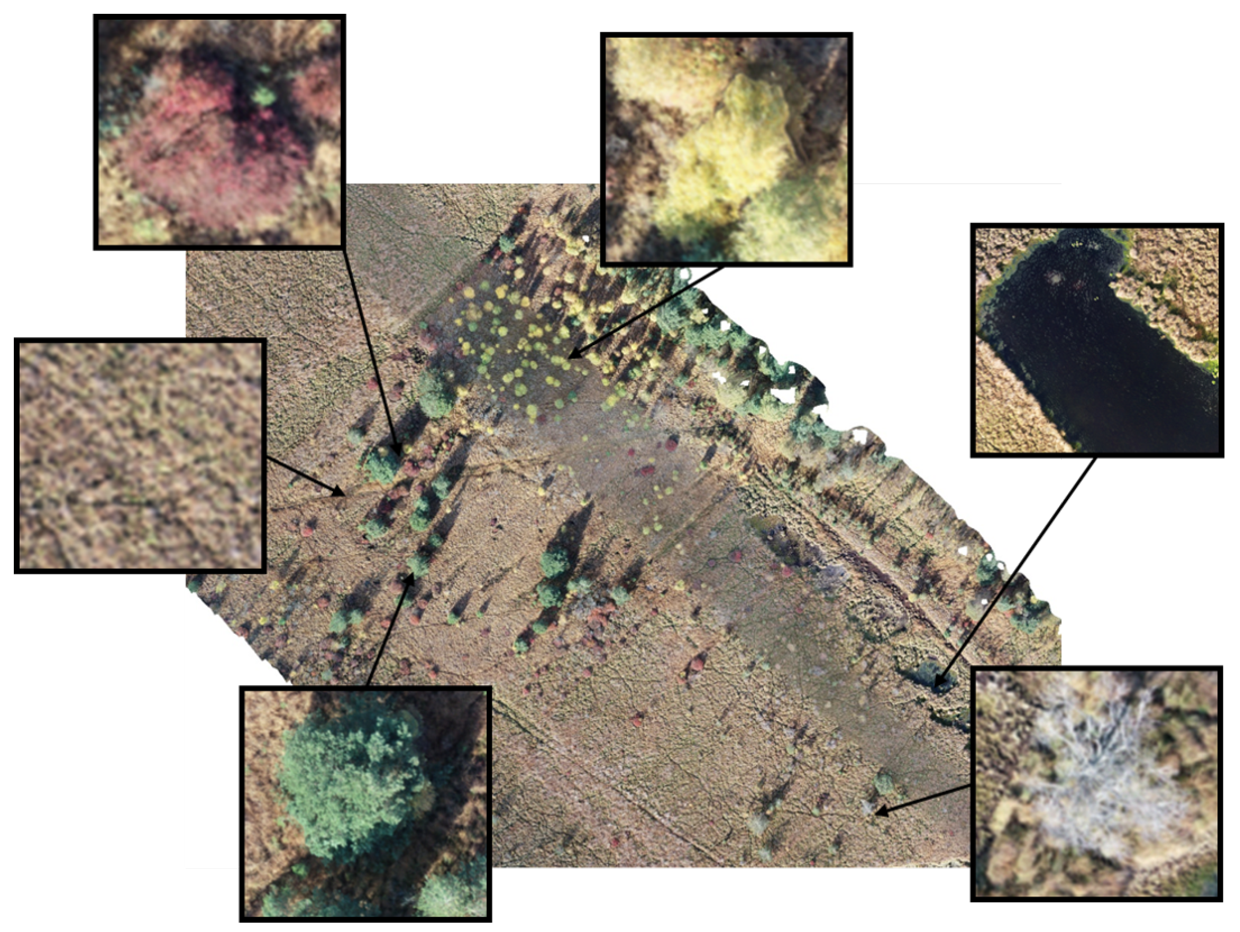
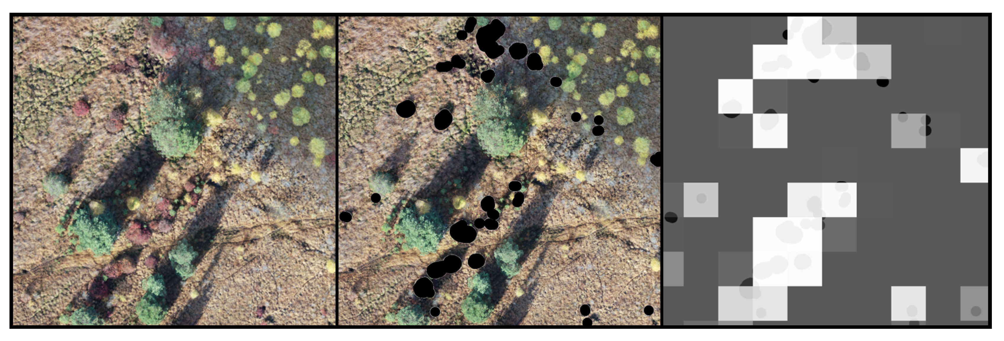
In this section, we present our dataset and the different methods that were used in our experiments. First, the area where the data was acquired is described along with a detailed explanation of the different classes visible in the images. Afterwards, the data preprocessing steps to obtain the mosaics are mentioned. Finally, we present our general DL framework consisting of different network architectures and data augmentation techniques for TL.

2.1. Data

Image collection was done in a natural environment defined as an “ombrotrophic bog”, i.e., a wetland hydrologically isolated from its environment receiving both water and nutrients exclusively from precipitation. As the quality of these environments is vulnerable to the impact of anthropogenic activities, a biodiversity protection program limits in situ field research as it is a standard in wetland protected areas around the world. Therefore, images were collected for the “Lichtenmoor” wetland (Figure 1, which is located about 60 km northwest of Hanover, in Germany (5243${}^{\prime }$06.2${}^{″}$N 920${}^{\prime }$41.5${}^{″}$E), by using a DJI phantom 4 drone in autumn 2018 taking advantage of seasonal red coloring of the blueberry leaves. Three flights were conducted where approximately 350 images each were gathered. The flights were conducted on one single day during the afternoon. The weather was sunny, which resulted in bright spots and long shadows within the orthomosaic. These images where then processed using the Metashape software [28] to produce one orthomosaic for each site. The orthomosaics covered between 10.6 to 12.4 ha of the wetland and produced images of around 10,000 square pixels.

On these 3 orthomosaics 6 classes were identified: blueberries, trees, yellow bushes, soil, water, and dead trees (Figure 2). The class trees contains pine trees (Pinus sylvestris), the class yellow bushes is defined by shrubby birches (predominantly Betula pubescens, secondary Betula pendula). However, as the purpose of these data is to detect the invasive blueberries within the images, the main focus was on their distribution and occurrence. Blueberries, especially, show a characteristic red color, which makes them easily recognizable and identifiable in comparison to other classes such as trees or bushes. In contrast to this, partly visible soil that appears in reddish tones hinder the blueberry classification. Furthermore, blueberries occur less frequently than other classes and in relatively small areas. This can be seen in Figure 2, where the mentioned highly unbalanced classes are visible. This imbalance is the highest when comparing blueberry and soil class. The three orthomosaics were divided into axis-parallel patches of side length (referred from now on as “patch size” = 100). In orthomosaic 1:162 out of 6400 patches contained blueberries while 2383 out of 6400 contained soil. For the orthomosaics 2 and 3, respectively, these numbers were 378/14,641 blueberry, 4254/14641 soil, and 222/7921 blueberry 2646/7921 soil. On average 2.64% of the patches over the three orthomosaics contained blueberry while 33.23% contained soil, thus the soil class is approximately 12.5 times more frequent than the blueberry class.

Annotation and Dataset Construction

The three orthomosaics obtained were annotated by experts using the open source image edition software GIMP [29]. Binary layers for each of the six classes were annotated in each of the three orthomosaics. These annotations were based on color, shape and context information.

The orthomosaics, as well as the annotation binary layers, were divided into squared patches of the same side length (given the size of the blueberry bushes, ranging from 20 to 100 pixels in radius, we decided to use s = 100 pixels for all the experiments presented). Therefore, patches of 100 × 100 pixels were used as an input for the DL network. In the first step of the network, each patch was resized to fit the size needed by each feature extractor. The classes present in each patch were stored in a separate “label” list. In general, patches contained more than one class and therefore formalized the problem as a multi-label patch classification problem.

2.2. Definition of the DL Network

The general structure of the DL approach has two main blocks. The first block comprises a well-known public architecture chosen among those included in the torchvision package of pytorch. As a TL approach was used, this block is considered the Feature Extractor and pretrained weights from the ImageNet data set were used to initialize the networks, unless stated explicitly. The second block is composed of two independent linear layers that substitute the original last layer of the pretrained networks. Each of these two layers is followed by a sigmoid activation function to impose independence between the different labels that may occur in a patch. The first output represents the probability of a patch to contain a certain label, while the second output is used to determine the percentage of pixels that belong to the class. The idea is to implicitly enforce the network to take into account classes with a low pixel count.

Regarding the feature extractors, the following architectures were considered as defined on the torchvision package from pytorch (A description of the implementation of each model and a quantitative comparison on the ImageNet dataset can be found at https://pytorch.org/docs/stable/torchvision/models.html):

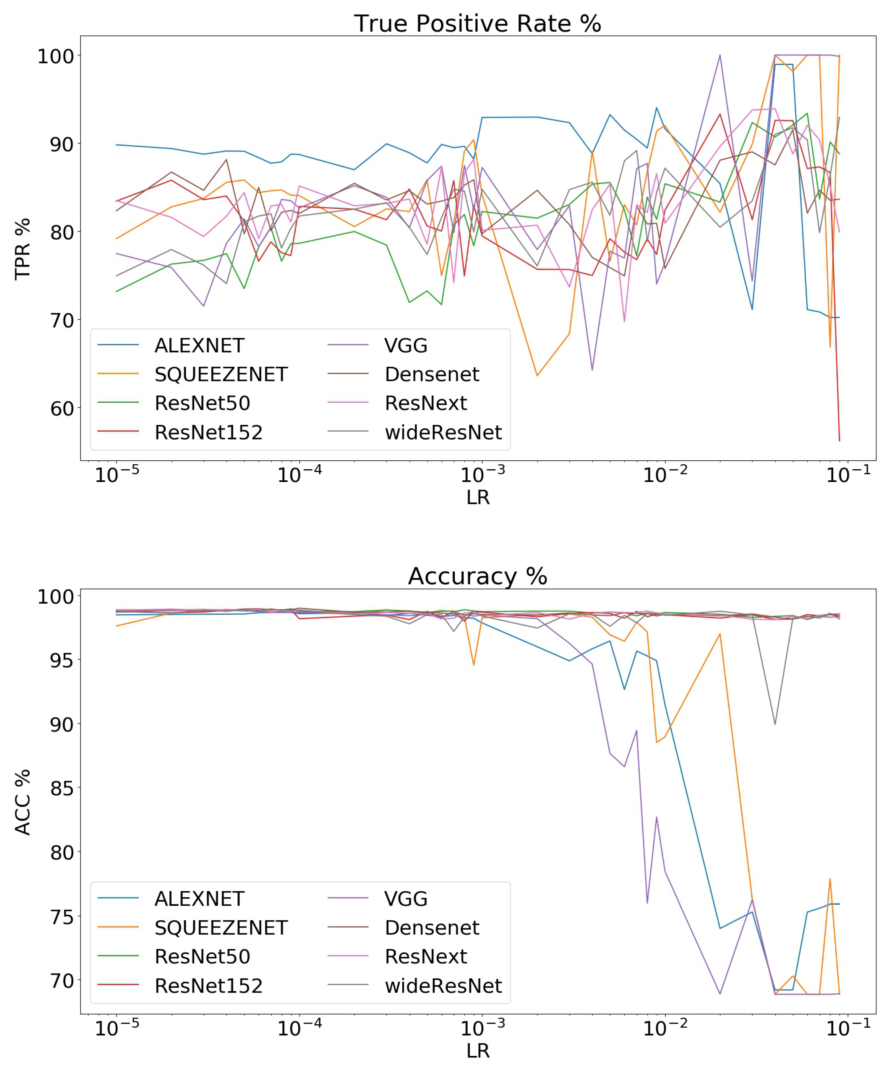
• Alexnet (alexnet) [18] is one of the first widely used convolutional neural networks, composed of eight layers (five convolutional layers sometimes followed by max-pooling layers and three fully connected layers). This network was the one that started the current DL trend after outperforming the current state-of-the-art method on the ImageNet data set by a large margin.
• VGG (vgg19_bn) [20] represents an evolution of the Alexnet network that allowed for an increased number of layers (19 with batch normalization in the version considered in our work) by using smaller convolutional filters.
• ResNet (resnet50, resnet152) [21] was one of the first DL architectures to allow higher number of layers by including blocks composed of convolution, batch normalization, and ReLU. Two versions with 50 and 152 layers, respectively, were used.
• Squeezenet (squeezenet1_0) [19] used so-called squeeze filters, including point-wise filter to reduce the number of parameters needed. A similar accuracy to Alexnet was claimed with fewer parameters.
• Densenet (densenet161) [22] uses a larger number of connections between layers to claim increased parameter efficiency and better feature propagation that allows them to work with even more layers (161 in this work).
• Wide ResNets (wide_resnet101_2) [24] tweak the basic architecture of regular ResNets to add more feature maps in each layer (increase width) while reducing the number of layers (network depth) in the hopes of ameliorating problems such as diminishing feature reuse.
• ResNeXt (resnext101_32x8d) [23] is a modification of the ResNet network that seeks to present a simple design that is easy to apply to practical problems. Specifically, the architecture has only a few hyper-parameters, with the most important being the cardinality (i.e., the number of independent paths, in the model).

According to a recent study in medical image segmentation [30], the first layers of an encoder–decoder are the ones that encode differences between image domains. In our case, we can clearly differentiate between the ImageNet domain and our own domain (aerial image orthomosaics). Therefore, different training strategies were used where the weights of different parts of the network were updated to test the best TL approach for our problem. Finally, to train all these networks, the Adam optimizer [31] and a one fit cycle learning rate scheduler to speed up convergence [32] were used.

2.3. Data Augmentation and Transfer Learning

Data augmentation is a commonly used strategy in DL that makes it possible to increase the size of all or part of the data set without the need to collect new data. It also allows to extend the dataset to unseen images by applying some transformations that can improve generalization. By making copies with simple image transformations of the blueberry patches the distribution of the training set can be altered and thus, shift the focus of the trained DL networks. The following image transformations to augment our data were applied.

• Small central rotations with a random angle. Depending on the orientation of the UAV, different orthomosaics acquired during different time frames might show different perspectives of the same trees. In order to introduce invariance to these differences, flips on the two main image axes can be applied to artificially increase the number of samples.
• Flips on the X and Y axes (up/down and left/right). Another way of addressing these differences is to mirror the image on their main axes (up/down, left/right).
• Gaussian blurring of the images. Due to the acquisition (movement, sensor characteristics, distance, etc.) and mosaicing process, some regions of the image might also present some blurring. Simulating these blurring with a Gaussian kernel to artificially expand the training dataset can also be used to simulate these issues and improve generalization.
• Linear and small contrast changes. Similarly, different lightning or shadows between regions of the image might also affect the results. By introducing these contrast changes, these effects can be stimulated and enlarge the number of training samples.
• Localized elastic deformation. Finally, elastic deformation were applied to simulate the possible different intra-species shapes of the blueberry patches.

To implement this transformations, the “imgaug” library [33] was used. This is expected to increase the classification accuracy of the images containing the augmented classes at the cost of decreasing that of other classes. Thus, in our case data augmentation was used to highlight the blueberry class which needed to be identified (see Section 3.1 for details).

Additionally advantages of the transfer learning (TL) capabilities of DL networks were taken. Whenever the available dataset is not sufficient to properly optimize the DL architecture being used, a commonly used technique is to initialize this structure using pre-loaded weights. These weights are typically the result of training the network to solve some related problem. Frequently, for classification purposes, optimized nets for the ImageNet dataset [18] are used. Some recent studies have detailed the benefits of TL [9,34,35].

2.4. Evaluation Criteria

In order to target the predictive capacity of our algorithms patch labels for the algorithm were considered. For all patches, the relation between predicted values and real values was considered as stated in the ground truth and broke into the usual classifications of True Positives: TP, False Positives: FP, True Negatives: TN, False Negatives: FN. Furthermore, in order to focus on the blueberry class, the following measures were computed on them (unless explicitly stated).

$$\begin{array}{c}TPR=SENS=\frac{\mathrm{TP}}{\mathrm{TP}+\mathrm{FN}}FPR=1-SPEC=\frac{\mathrm{FP}}{\mathrm{TN}+\mathrm{FP}}\\ ACC=\frac{\mathrm{TP}+\mathrm{TN}}{\mathrm{TP}+\mathrm{TN}+\mathrm{FP}+\mathrm{FN}}\end{array}$$

(1)

3. Results

In this section, experiments were presented using real data corresponding to three orthomosaics constructed using the UAV data acquired. All algorithms described throughout the paper were implemented using the python programming language [36] and the pytorch Library [37]. All experiments where run using a Linux Ubuntu operating system with 10 dual-core 3GHz processors and an NVIDIA GTX 1080 graphics board. Figure 3 shows an example of the annotated data and the result produced by the ResNet50 network.

The three orthomosaics available were divided into two for training/validation while and a the third one for testing. The orthomosaic used for testing was rotated so all orthomosaics were used for testing once and no orthomosaic was used for training/validation and testing at the same time to avoid leakage between the training and testing patches. This is usually known as a leave-one-out strategy and resulted in the following training/testing set combination.

• First fold, testing: Orthomosaic 1, (6400 patches, with 2.53% blueberry), Training: Orthomosaics 2,3 (22,562 patches with 2.66 blueberry)
• Second fold, testing: Orthomosaic 2, (14,641 patches, with 2.58% blueberry), Training: Orthomosaics 1,3 (14,321 patches with 2.68 blueberry)
• Third fold, testing: Orthomosaic 3, (7921 patches, with 2.53% blueberry), Training: Orthomosaics 1,2 (21,041 patches with 2.57 blueberry)

The results presented in this section are averages for the TPR, FPR and accuracy results for the Blueberry class of the three testing stages. Regarding the other classes, our experiments showed that training the network to classify them helped to improve the classification of the blueberry class. Infrequent classes (trees, yellow bushes, water, and dead trees) appeared to follow the same tendencies as the blueberry class while the much more frequent soil class tended to get higher TPR and lower accuracy. The networks used in this study could undoubtedly also be tailored to detect these classes, however this remains out of the scope of the present work.

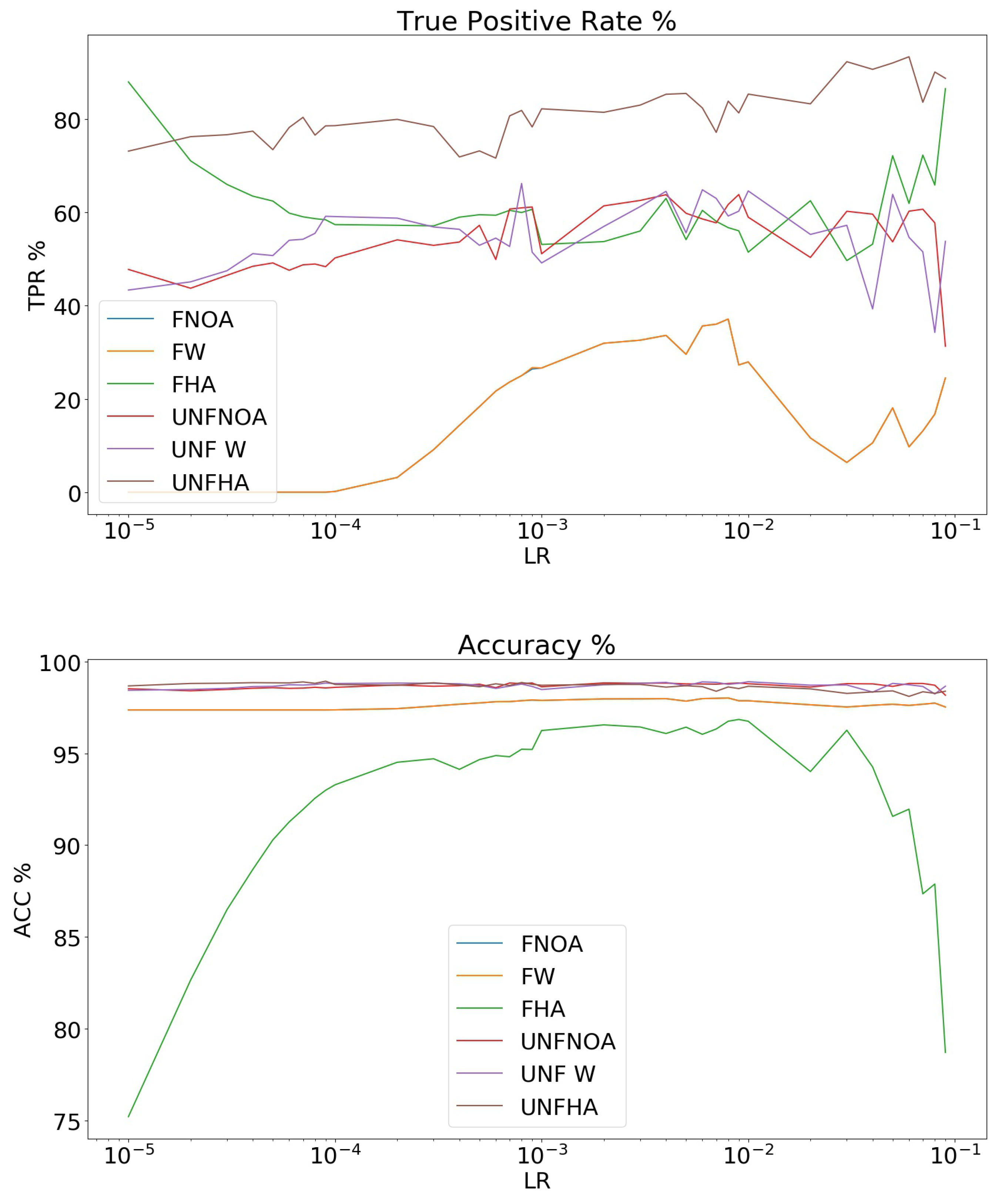
3.1. Data Balancing and TL

In this experiment a network (ResNet 50 [21]) was chosen that has been used to solve a variety of classification problems. Our main focus here is to study how this network can be adapted to solve our practical problem.

Usually all the images in the training set have the same importance. In a multi-label classification case, each training sample will have the same contribution on the loss function and within it, determining correctly the presence or absence of each possible label will also have the same importance. Consequently, networks usually present a bias towards the most frequent classes. Once enough examples have been seen by the network, it should learn to properly classify all the different classes. However, if not enough examples of a pattern (for example, an infrequent class appearing in a patch) are seen by a network, the network may not learn to accurately predict these occurrences.

As discussed in Section 2.1, our problem presents a severe imbalance between the classes, especially as the blueberry class is a very infrequent class (appearing in 2.64% of patches). As the results show, using the ResNet without adapting it to the problem characteristics results in a low detection rate for the blueberry class. In order to obtain a higher detection rate for this class two main approaches were applied:

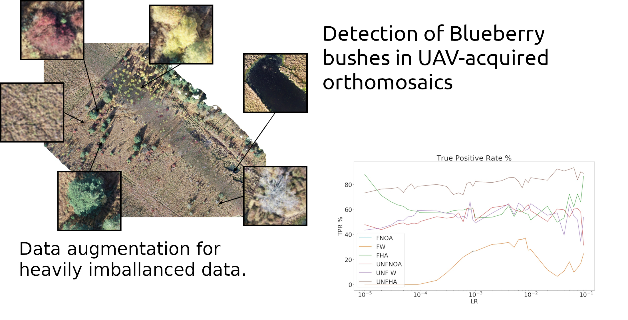
• Loss function Weighting. By giving different weights to the different classes in the loss function the relative importance of each class can be altered. However, this is not enough, as correctly detecting the presence of a class contributes the same as correctly detecting its absence: A network that does not predict the blueberry class in any patch will still be right over 97% of times. Consequently, even with loss function weighting, infrequent classes will remain underpredicted.
• Data augmentation: By making copies with simple transformations (see Section 2.3) of the blueberry patches the distribution of the training set can be altered and thus, increase the importance of classes in the loss function. This is expected to increase the classification accuracy of the patches containing the augmented classes while decreasing that of other classes.

Regarding TL, we initially used weights trained on the ImageNet dataset [18] to initialize our network. These networks were considered frozen and unfrozen. The term frozen here stands for a network where all layers except the final (classification) one are kept unchanged during training. Conversely, in unfrozen networks, all layers are trained and their weights are allowed to change. The goals here were to assess whether frozen networks with ImageNet weights were able to adequately solve our problem and to quantify the importance of these pretrained weights against random weights. Frozen and unfrozen versions of the ResNet network were considered except for the case of a network initialized with random weights.

To test the effect of data augmentation on the data imbalance, several possibilities were considered concerning the training data sets and include representative examples of the main tendencies observed:

• No augmentation and no weighting of the loss function. This network was considered frozen FNOA and unfrozen UNFNOA.
• Only weighting of the loss function, with no data augmentation, FW and UNFW. In this case, the weights for the six classes were [6,2,2,1,2,2] in order to give more importance to the blueberry class and less to the soil class.
• Weighting of the loss function [8,2,2,1,2,2]. The blueberry class was, thus, assigned a weight of “8”, the soil class a weight of “1”, and the rest of classes a weight of “2”. A “high level” of data augmentation was used, naming the data sets FHA and UNFHA. Twelve new images for each image of the blueberry class was created.

Another important aspect of TL approaches, is the learning rate of a DL model. This parameter controls the step size of the optimizer that changes the weights in each iteration of the training phase. In order to analyze how it affected TL, a set of experiments with different values were performed. A comprehensive picture is presented, among all values tested from $1\times {10}^{-5}$ to $0.09$ with 10 sampling points at each exponent value ($1\times {10}^{-5},2\times {10}^{-5}\dots 9\times {10}^{-5},1\times {10}^{-4},2\times {10}^{-4}\dots$). Figure 4 shows the TPR, and accuracy values for the classification of Blueberry patches with the different training data sets. FPR was left out of the Figure as its evolution determines accuracy to such an extent that the two FPR and accuracy Figures show basically the same trends. In order to provide some more details on the differences of behavior for the different training sets,

Table 1. Summary of values for all learning rates considered and the different training modes: F stands for Frozen and UNF for unfrozen in the following cases: Without data augmentation or loss function weighting (FNOA and UNFNOA), only with loss function weighting (FW and UNFW), and with function weighting and intensive use of data augmentation (FHA and UNFHA).

	TPR			FPR			ACC
	Best	Mean	Stdev	Best	Mean	Stdev	Best	Mean	Stdev
FNOA	37.13	15.86	13.05	0.00	0.13	0.14	98.01	97.66	0.24
FW	37.13	15.87	13.06	0.00	0.13	0.14	98.01	97.66	0.24
FHA	87.99	61.24	8.25	2.04	6.66	5.45	96.84	92.49	5.10
UNFNOA	63.83	54.55	7.05	0.02	0.13	0.04	98.83	98.68	0.15
UNF W	66.21	54.98	7.11	0.04	0.12	0.07	98.90	98.69	0.15
UNFHA	93.39	81.31	5.85	0.47	0.89	0.35	98.93	98.64	0.21

provides details on best and average values for TPR, FPR, and accuracy.

In order to limit the effects of randomness, all tests were run with the same seeds for all the pseudo-random generators used. This has two main practical effects: First, all of the presented data sets are fixed for the test run with all the learning rates. Second, the order in which the images are fed into the network is always the same. By removing these sources of randomness, it was ensured that the differences should only occur from the balancing approaches.

The inverse trends observed between the FPR and accuracy happened due to the data imbalance: as the results correspond to testing sets where the percentage of patches of each class has not been altered, there are many more patches not containing the blueberry class than those containing it. Consequently, low FPR values also imply high accuracy. These accuracy values need to be properly contextualized. For example, for orthomosaic 2, a classifier that predicts all patches to be negative respect to the blueberry class will still reach approximately 97% classification accuracy. This happens because only 2.53% of the patches in this orthomosaic contain the blueberry class.

The primarily interested was in finding the patches that actually do contain the blueberry class, TPR and FPR were provided. Consequently, instances of the network should have high TPR with FPR as low as possible. Therefore, networks are considered successful if their TPR is above 90% while the absolute number of FP is lower than the absolute number of TP. This usually stands for a FPR under 2% (the TPR is computed over the number of patches containing Blueberries while the FPR is computed over the total number of patches).

Taking this into account, it can be seen that frozen versions of the network perform worse than the unfrozen ones. Most frozen networks have problems finding the patches containing the blueberry class and present a low (<60) TPR. An exception to this is the FHA version of the network that achieves high TPR for some LR values at the cost of noticeably increasing its FPR and, thus, decreasing the accuracy. Apart from this case, the other frozen networks achieve high accuracy values (over 97% for the FNOA and FW networks) but their relatively low capacity to detect the patches containing the blueberry class makes them unsuitable for our application. This issue shows that using ImageNet weights to solve our problem directly with minimal retraining is not a feasible option. Although the networks thus trained can still obtain high accuracy values, they do not provide sufficiently high blueberry TPR. The reason for this may be that the ImageNet data set is trained to provide the best overall classification accuracy for all classes and, thus does not account for this type of unbalanced data set. Furthermore, this also reinforces the findings of a recent paper [30] that suggests that domain differences are encoded on the first layers of the network. By only training the final (classification) layer, the network cannot properly adapt to the domain differences between the ImageNet dataset and our own.

Conversely, the unfrozen networks prove more adaptable to our needs in the problem and provided a high TPR while still retaining a low FPR and high accuracy. When no data augmentation was used,(UNFNOA and UNFW). Although accuracies over 98% where achieved for the blueberry class, TPR values remained low (with a maximum of 63.8% for UNFNOA and 66.21% for UNFW). When data augmentation was used, it was possible to achieve a higher TPR at the cost of also increasing the FPR. The best accuracy value of 98.92% with 78.56% TPR for a LR of 0.00009 was obtained by the UNFHA network. The same network showed a tendency to increase both the TPR and FPR with the majority of the learning rates. In terms of results obtaining a high TPR value while keeping high accuracy, the UNFHA network obtained 93.39% TPR with accuracy 98.10% for LR 0.06.

Finally, it was tested whether or not the use of the ImageNet weights in the unfrozen networks made a difference in order to solve the problem. The same test was run for the different learning rates with the UNFHA data set that used data augmentation. In this case, however, the ResNet50 network was initialized with random weights.

Table 2. Summary of values of the UNFHA training set when the ResNet50 network is initialized with ImageNet and random weights.

	TPR			FPR			ACC
	Best	Mean	Stdev	Best	Mean	Stdev	Best	Mean	Stdev
ImageNet Weights	93.28	81.31	5.85	0.47	0.88	0.34	98.92	98.64	0.21
Random Weights	92.58	83.88	7.66	0.79	1.33	0.46	98.63	98.27	0.53

shows a summary of the results obtained with the best, average and standard deviation values for the three metrics considered.

The results show that the network initialized with random weights achieves results close to those achieved with the ImageNet weights. Using random weights results in higher variances for the three metrics and slightly lower accuracy (the difference was statistically significant by using a difference of mean paired-samples t-test with 99% confidence level with a p-value of 0.0056). This pattern was also observed for the FPR metric. In terms of TPR the best average was obtained by using random weights.

Statistical Significance of the Results

The experiments described so far were run with fixed pseudo-random seeds in order to limit the random effects during training. In the following paragraphs a brief discussion and quantify the importance of these effects were made. Two main sources of randomness were considered: (1) In the absence of data augmentation, all the patches in two orthomosaics were used as the training set and all the patches in the third orthomosaic as the testing set in a leave-one-orthomosaic-out strategy. Consequently, in each fold of the leave-one-orthomosaic-out the training and testing sets were fixed. The order in which the network sees the training patches was not fixed as the data loader randomly shuffles the training patches at each epoch. (2) If data augmentation was used, upsampling and downsampling have a random component. In particular, data augmentation always generates the same number of images but with random transformations (flips, blurring, etc.). Consequently, in each execution the distribution of the training sets is different if the random seed is not fixed.

In order to test the relative importance of these two sources of random effects, the seed for the pseudo-random number generators was not fixed and run the ResNet50 networks with a fixed learning rate (LR = 0.06) A) without data augmentation (to evaluate the effect of the shuffle in the training set in the final result) and B) with data augmentation as described for the UNFHA set. The test was repeated 25 times and observed differences due to random effects are presented in

Table 3. Summary of values of running the UNFNOA and UNFHA training sets repeatedly to assess the extent of random effects.

	TPR			FPR			ACC
	Best	Mean	Stdev	Best	Mean	Stdev	Best	Mean	Stdev
UNFNOA	66.05	52.05	11.25	0.09	0.19	0.13	98.87	98.53	0.30
UNFHA	92.47	81.44	9.35	0.57	1.21	0.39	98.54	98.33	0.23

.

The first row in Table 3 summarizes the variability observed for the case that does not use data augmentation. This variability is due to the order in which the training data is processed by the network. The second row illustrates the variability observed when using data augmentation and containing, in addition to the effect previously mentioned, the random effects caused by the production of augmented images or the downsampling of the most frequent class.

The fact that the standard deviation observed for the accuracy and TPR values is larger for the case without augmentation shows the importance of order in which the patches are read by the network. In particular, as the initial steps of training involve larger weight updates (higher loss), few examples of the blueberry class will hamper the ability of the network to correctly recognize it. This problem is mitigated by using data augmentation as can be seen by the lower variances in both metrics for the first row in Table 3. As a consequence, however, the bias towards the blueberry class results in an increased average value for the FPR (jumping from 0.09 to 0.57 when using data augmentation with increased variability as shown by the 0.39 stdev value for UNFHA).

Finally, the use of data augmentation produces an increase in TPR that is greater than the differences attributed to random variability. This is evident by the jump from 66.05% TPR to 92.47% when using data augmentation is much larger than the standard deviation observed due to randomness (11.25%). This difference was found to be statistically significant with 99% confidence level with $p\text{-}\mathrm{value}<<0.001$.

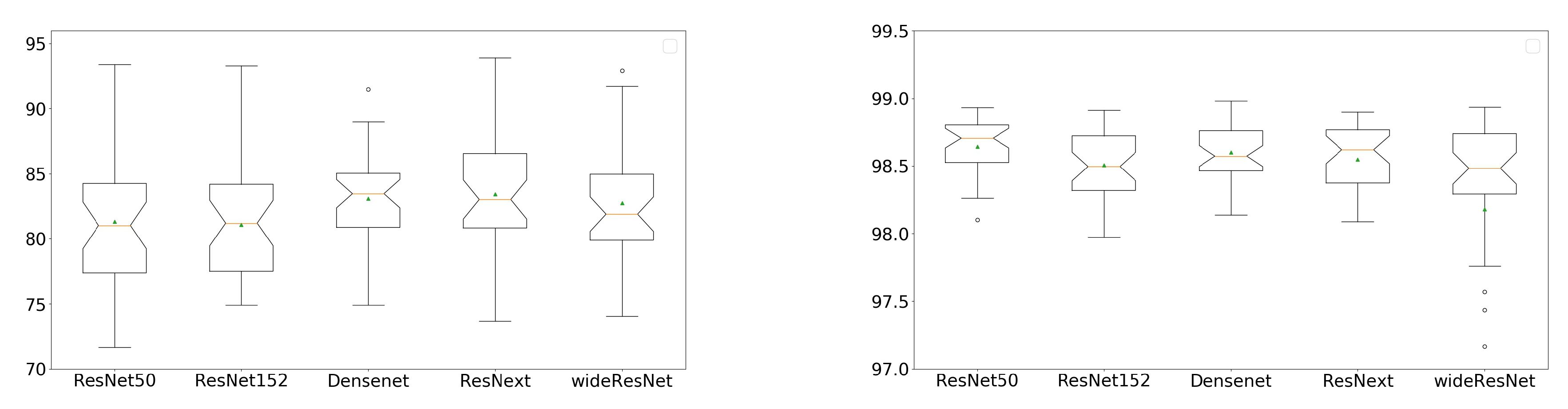
3.2. Comparison of Different Networks

For this experiment the effect of randomness were limited by choosing the same seed for all the pseudo-random generators. This ensures that all the networks were trained on the exact same data distribution (i.e., all the images were exactly the same and were read in the same order) and tested on the same testing data set.

In this case, as already seen in Figure 4, due to data imbalance the FPR determined the accuracy so the FPR and accuracy Figures showed the same tendencies. Consequently, Figure 5 shows TPR and accuracy results for all the networks and learning rates studied with the FPR curve left out for the sake of brevity.

The results show that some networks fail to produce satisfactory results for some learning rates. A very large number of FP compromise their overall accuracy rendering them unusable in practice. This behavior is observed for larger learning rates for Alexnet, Squeezenet, and VGG, and for a learning rate of 0.04 for wideResNet. Densenet and the ResNet-based networks follow a much better trend with high TPR as well as high accuracy. In order to tell their behavior apart, Figure 6 presents boxplots summarizing their performance.

In terms of accuracy, the best values were obtained by Densenet with 98.98. wideResNet (98.93), ResNet50 (98.92), ResNet152 (98.91), VGG (98.90), and ResNeXt (98.90) were close in terms of best accuracy. Finally, Squeezenet achieved the best accuracy of 98.89 and Alexnet of 98.65. The average and stdev values for the accuracy metric show that adequate results were achieved, whereby lower averages in accuracy were accompanied by higher variances. The extent was high for Alexnet (mean = 92.05, stdev = 10.14), Squeezenet (92.42, 10.85), VGG (89.49, 12.24), and smaller for wideResnet (98.18, 1.48) were the problem was only present in one of the three orthomosaics of the LR = 0.4-fold. Higher average accuracy values were obtained (in increasing order) by ResNet152 (98.64, 0.25), ResNeXt (98.54, 0.25), Densenet (98.60, 0.20), and finally ResNet50 (98.64,0.20). Regarding the statistical significance of the accuracy results observed, pairwise difference of means t-tests with paired data were performed with a 99% level of confidence (

Table 4. Summary of results of the pairwise difference of means (paired data) t-tests.

Level 0	Squeezenet	AlexNet
Level 1	Vgg
Level 2	ResNet152	ResNeXt	wideResNet
Level 3	ResNet50	Densenet

). Methods that were not found to perform significantly different were put in the same level. With a higher level denoting significantly higher mean. In the case of wideResNet, its larger variance meant that its performance could not be told apart from methods from two separate levels.

In terms of TPR, results were considered where the accuracy was over 98% as results with a large number of FP are not of practical use. Taking this into account, the best TPR results always came at the cost of slightly increased FPR and, thus, decreased accuracy. The best results with these restrictions were obtained by ResNeXt (TPR = 93.75, Acc = 98.11) ResNet50 (93.39, 98.10), and ResNet152 (92.54, 98.13). Similar results were also obtained by Densenet (91.50, 98.14) and wideResNet (91.73, 98.19). Squeezenet, Alexnet, and VGG topped at 90.29%, 89.80%, and 87.23% TPR, respectively.

4. Discussion

The results in Section 3.1 show that the ResNet50 network succeeded at the classification tasks associated to our problem. The best results were obtained by retraining the whole network (as opposed to only the final layers as commonly done). In this respect, relying on TL to solve our problem after only a minor retraining of the last layer is shown to be suboptimal. A data set that is large enough to retrain the full networks is, thus, shown to be necessary to obtain the best results. Moreover, the needed large changes of the whole network resulted in a small benefit to initializing with the ImageNet weights as opposed to random weights. Although the network initialized with random weights had a less stable behavior (as shown by a larger variance observed in its accuracy over all learning rates) and a statistically significantly smaller accuracy, it was able to obtain the best average value for the TPR metric.

At the same time, the results also quantify how the imbalance in the labels may result in a network that classifies most patches correctly while not providing a solution that of practical use. This happens in situations where the minority classes are important. To solve this problem, the use of weights in the loss function was shown as well as data augmentation, which helped to bias the training distribution towards a result that served our interests. Even though we arbitrarily defined these interests as high TPR with FPR under 1%, the results show that the methodology used in this experiment can accommodate different use cases. For example, to know whether or not a particular area has been infested by blueberries, then the UNFNOA or UNFW networks will need to find roughly 65% of the blueberries present while adding very few (under 0.2%) false positive detections. On the other hand, to find as many of the blueberries as possible, the UNFHA network will find 93% of them by adding 1.77% of FP.

In Section 3.2 different DL networks with the same training and testing data sets were tested in order to limit the importance of random effects. The testing run-times of these networks were pretty uniform and fast (under three minutes to process the images in one orthomosaic). Their training times varied greatly with the architecture and reached, for example, more than three hours for larger networks such as wideResNet, around 25 minutes for a mid-sized network such as ResNet50 and a little over 8 minutes for small networks such as ALEXNET. The best results in terms of accuracy were obtained by the Densenet network (best accuracy for the three folds) and the ResNet50 network (best average accuracy throughout all the learning rate values). However, ResNet50, Densenet, and wideResNet achieved similar results that did not present statistically significant differences. In terms of TPR, results were considered as optimal if they had accuracy values over 98% in order to limit the number of FP. Results over 90% TPR with an accuracy over 98% were achieved showing that the networks studied can use the data augmentation considered to effectively solve the problem of detecting the invasive blueberry in wetland orthomosaics. Best overall results were obtained by ResNeXt (TPR = 93.75, Acc = 98.11) with ResNet50, ResNet152, Densenet, and wideResNet obtaining similar (albeit slightly lower in terms of TPR results).

5. Conclusions and Future Work

We have shown that DL networks can be used to detect the presence of invasive blueberry bushes in German wetlands. However, in order to achieve results that are of practical use, we needed to modify the training sets by using data augmentation and loss function weighting. Our results were shown to be statistically significant and the effect of randomness in training was also quantified.

In future work, we will explore the use of multichannel data (such as RGB + digital elevation maps or multispectral data), machine learning-focused phenotyping techniques, and our pixel percentage output to help achieve a semantic segmentation of orthomosaics [38]. We would also like to consider the use of other loss functions for data balance, such as the focal loss. In order to improve the effectiveness of the data augmentation used, we will also consider data augmentation using generative adversarial networks (GANs) to generate new samples of blueberry patches. This type of approach, where a generative network is trained to create new samples that follow the distribution of the training dataset by fooling a network that discriminates between real and fake samples, has been recently applied to medical imaging with great success [39,40]. Finally, we want to use the automatic blueberry detection results produced by our networks to track the spread of the invasive blueberry species over orthomosaics of the same site taken in different years.

References

1. Prentis, P.J.; Wilson, J.R.; Dormontt, E.E.; Richardson, D.M.; Lowe, A.J. Adaptive evolution in invasive species. Trends Plant Sci. 2008, 13, 288–294. [Google Scholar] [CrossRef] [PubMed]
2. Pyšek, P.; Richardson, D.M. Invasive Species, Environmental Change and Management, and Health. Annu. Rev. Environ. Resour. 2010, 35, 25–55. [Google Scholar] [CrossRef] [Green Version]
3. Pimentel, D.; Zuniga, R.; Morrison, D. Update on the environmental and economic costs associated with alien-invasive species in the United States. Ecol. Econ. 2005, 52, 273–288. [Google Scholar] [CrossRef]
4. Grenzdorffer, G.; Teichert, B. The photogrammetric potential of low-cost UAVs in forestry and agriculture. Int. Arch. Photogramm. Remote Sens. Spatial Inf. Sci. 2008, 31, 1207–1214. [Google Scholar]
5. Raparelli, E.; Bajocco, S. A bibliometric analysis on the use of unmanned aerial vehicles in agricultural and forestry studies. Int. J. Remote Sens. 2019, 40, 9070–9083. [Google Scholar] [CrossRef]
6. Tang, L.; Shao, G. Drone remote sensing for forestry research and practices. J. For. Res. 2015, 26, 791–797. [Google Scholar] [CrossRef]
7. Natesan, S.; Armenakis, C.; Vepakomma, U. Resnet-Based Tree Species Classification Using Uav Images. ISPRS-Int. Arch. Photogramm. Remote. Sens. Spat. Inf. Sci. 2019, XLII-2/W13, 475–481. [Google Scholar] [CrossRef] [Green Version]
8. Gambella, F.; Sistu, L.; Piccirilli, D.; Corposanto, S.; Caria, M.; Arcangeletti, E.; Proto, A.R.; Chessa, G.; Pazzona, A. Forest and UAV: A bibliometric review. Contemp. Eng. Sci. 2016, 9, 1359–1370. [Google Scholar] [CrossRef]
9. Kentsch, S.; Lopez Caceres, M.L.; Serrano, D.; Roure, F.; Diez, Y. Computer Vision and Deep Learning Techniques for the Analysis of Drone-Acquired Forest Images, a Transfer Learning Study. Remote Sens. 2020, 12, 1287. [Google Scholar] [CrossRef] [Green Version]
10. Sa, I.; Chen, Z.; Popović, M.; Khanna, R.; Liebisch, F.; Nieto, J.; Siegwart, R. weedNet: Dense Semantic Weed Classification Using Multispectral Images and MAV for Smart Farming. IEEE Robot. Autom. Lett. 2018, 3, 588–595. [Google Scholar] [CrossRef] [Green Version]
11. Deng, L.; Yu, R. Pest recognition system based on bio-inspired filtering and LCP features. In Proceedings of the 2015 12th International Computer Conference on Wavelet Active Media Technology and Information Processing (ICCWAMTIP), Chengdu, China, 18–20 December 2015; pp. 202–204. [Google Scholar] [CrossRef]
12. Shiferaw, H.; Bewket, W.; Eckert, S. Performances of machine learning algorithms for mapping fractional cover of an invasive plant species in a dryland ecosystem. Ecol. Evol. 2019, 9, 2562–2574. [Google Scholar] [CrossRef] [PubMed] [Green Version]
13. Stieper, L.C. Distribution of Wild Growing Cultivated Blueberries in Krähenmoor and Their Impact on Bog Vegetation and Bog Development. Bachelor’s Thesis, Institute of Physical Geography and Landscape Ecology, Leibniz University of Hannover, Hannover, Germany, 2018. [Google Scholar]
14. Schepker, H.; Kowarik, I.; Grave, E. Verwilderung nordamerikanischer Kultur-Heidelbeeren (Vaccinium subgen. Cyanococcus) in Niedersachsen und deren Einschätzung aus Naturschutzsicht. Nat. Und Landsch. 1997, 72, 346–351. [Google Scholar]
15. Krizhevsky, A.; Sutskever, I.; Hinton, G.E. ImageNet Classification with Deep Convolutional Neural Networks. In Advances in Neural Information Processing Systems 25; Pereira, F., Burges, C.J.C., Bottou, L., Weinberger, K.Q., Eds.; Curran Associates, Inc.: Red Hook, NY, USA, 2012; pp. 1097–1105. [Google Scholar]
16. Dupret, G.; Koda, M. Bootstrap re-sampling for unbalanced data in supervised learning. Eur. J. Oper. Res. 2001, 134, 141–156. [Google Scholar] [CrossRef]
17. He, H.; Garcia, E.A. Learning from Imbalanced Data. IEEE Trans. Knowl. Data Eng. 2009, 21, 1263–1284. [Google Scholar]
18. Krizhevsky, A.; Sutskever, I.; Hinton, G.E. ImageNet Classification with Deep Convolutional Neural Networks. Commun. ACM 2017, 60. [Google Scholar] [CrossRef]
19. Iandola, F.N.; Moskewicz, M.W.; Ashraf, K.; Han, S.; Dally, W.J.; Keutzer, K. SqueezeNet: AlexNet-level accuracy with 50x fewer parameters and <1 MB model size. arXiv 2016, arXiv:1602.07360. [Google Scholar]
20. Simonyan, K.; Zisserman, A. Very Deep Convolutional Networks for Large-Scale Image Recognition. In Proceedings of the International Conference on Learning Representations, San Diego, CA, USA, 7–9 May 2015. [Google Scholar]
21. He, K.; Zhang, X.; Ren, S.; Sun, J. Deep Residual Learning for Image Recognition. arXiv 2015, arXiv:1512.03385. [Google Scholar]
22. Huang, G.; Liu, Z.; Weinberger, K.Q. Densely Connected Convolutional Networks. In Proceedings of the 2017 IEEE Conf. on Computer Vision and Pattern Recognition (CVPR), Honolulu, HI, USA, 21–26 July 2017; pp. 2261–2269. [Google Scholar]
23. Xie, S.; Girshick, R.; Dollar, P.; Tu, Z.; He, K. Aggregated Residual Transformations for Deep Neural Networks. In Proceedings of the IEEE Conference on Computer Vision and Pattern Recognition (CVPR), Honolulu, HI, USA, 21–26 July 2017. [Google Scholar]
24. Zagoruyko, S.; Komodakis, N. Wide Residual Networks. In Proceedings of the British Machine Vision Conference (BMVC); Richard, C., Wilson, E.R.H., Smith, W.A.P., Eds.; BMVA Press: York, UK, 2016; pp. 87.1–87.12. [Google Scholar] [CrossRef] [Green Version]
25. Shorten, C.; Khoshgoftaar, T. A survey on Image Data Augmentation for Deep Learning. J. Big Data 2019, 6, 1–48. [Google Scholar] [CrossRef]
26. Zhao, X.; Zhang, J.; Tian, J.; Zhuo, L.; Zhang, J. Residual Dense Network Based on Channel-Spatial Attention for the Scene Classification of a High-Resolution Remote Sensing Image. Remote Sens. 2020, 12, 1887. [Google Scholar] [CrossRef]
27. Masarczyk, W.; Głomb, P.; Grabowski, B.; Ostaszewski, M. Effective Training of Deep Convolutional Neural Networks for Hyperspectral Image Classification through Artificial Labeling. Remote Sens. 2020, 12, 2653. [Google Scholar] [CrossRef]
28. Agisoft. Agisoft Metashape 1.5.5, Professional Edition. Available online: http://www.agisoft.com/downloads/installer/ (accessed on 19 August 2019).
29. Team, T.G. GNU Image Manipulation Program. 2020. Available online: http://gimp.org (accessed on 29 June 2020).
30. Shirokikh, B.; Zakazov, I.; Chernyavskiy, A.; Fedulova, I.; Belyaev, M. First U-Net Layers Contain More Domain Specific Information Than The Last Ones. In Proceedings of the DART workshop at the MICCAI Conference 2020, Lime, Peru, 4–8 October 2020. [Google Scholar]
31. Kingma, D.P.; Ba, J. Adam: A Method for Stochastic Optimization. arXiv 2014, arXiv:1412.6980. [Google Scholar]
32. Smith, L.N.; Topin, N. Super-Convergence: Very Fast Training of Neural Networks Using Large Learning Rates. arXiv 2017, arXiv:1708.07120. [Google Scholar]
33. Jung, A.B.; Wada, K.; Crall, J.; Tanaka, S.; Graving, J.; Reinders, C.; Yadav, S.; Banerjee, J.; Vecsei, G.; Kraft, A.; et al. Imgaug. 2020. Available online: https://github.com/aleju/imgaug (accessed on 1 July 2020).
34. Othmani, A.; Taleb, A.R.; Abdelkawy, H.; Hadid, A. Age estimation from faces using deep learning: A comparative analysis. Comput. Vis. Image Underst. 2020, 196, 102961. [Google Scholar] [CrossRef]
35. Malik, H.; Farooq, M.S.; Khelifi, A.; Abid, A.; Nasir Qureshi, J.; Hussain, M. A Comparison of Transfer Learning Performance Versus Health Experts in Disease Diagnosis From Medical Imaging. IEEE Access 2020, 8, 139367–139386. [Google Scholar] [CrossRef]
36. Van Rossum, G.; Drake, F.L., Jr. Python Tutorial; Centrum voor Wiskunde en Informatica: Amsterdam, The Netherlands, 1995. [Google Scholar]
37. Paszke, A.; Gross, S.; Massa, F.; Lerer, A.; Bradbury, J.; Chanan, G.; Killeen, T.; Lin, Z.; Gimelshein, N.; Antiga, L.; et al. PyTorch: An Imperative Style, High-Performance Deep Learning Library. In Advances in Neural Information Processing Systems 32; Wallach, H., Larochelle, H., Beygelzimer, A., dAlchéBuc, F., Fox, E., Garnett, R., Eds.; Curran Associates, Inc.: Red Hook, NY, USA, 2019; pp. 8024–8035. [Google Scholar]
38. Zaman-Allah, M.; Vergara, O.; Araus, J.L.; Tarekegne, A.; Magorokosho, C.; Zarco-Tejada, P.J.; Hornero, A.; Albà, A.H.; Das, B.; Craufurd, P.; et al. Unmanned aerial platform-based multi-spectral imaging for field phenotyping of maize. Plant Methods 2015, 11. [Google Scholar] [CrossRef] [Green Version]
39. Frid-Adar, M.; Diamant, I.; Klang, E.; Amitai, M.; Goldberger, J.; Greenspan, H. GAN-based synthetic medical image augmentation for increased CNN performance in liver lesion classification. Neurocomputing 2018, 321, 321–331. [Google Scholar] [CrossRef] [Green Version]
40. Sandfort, V.; Yan, K.; Pickhardt, P.J.; Summers, R.M. Data augmentation using generative adversarial networks (CycleGAN) to improve generalizability in CT segmentation tasks. Nat. Sci. Rep. 2019, 9. [Google Scholar] [CrossRef] [PubMed]
Figure 1. Location of data acquisition sites.
Remotesensing 12 03431 g001
Figure 2. Section of one of the orthomosaics studied, with detail of the different classes.
Remotesensing 12 03431 g002
Figure 3. Left, section of one of the orthomosaic. Center, the annotation mask for the blueberry class is highlighted in black. Right, the prediction mask is superimposed to the annotation mask, with black pixels representing a higher likelihood of containing the blueberry class.
Remotesensing 12 03431 g003
Figure 4. TPR (top) and accuracy (bottom) for the blueberry class. Data for training: F stands for Frozen and UNF for unfrozen in the following cases; without data augmentation or loss function weighting (FNOA and UNFNOA), only with loss function weighting (FW and UNFW), and with function weighting and intensive use of data augmentation (FHA and UNFHA).
Remotesensing 12 03431 g004
Figure 5. TPR (top) accuracy (bottom). Models studied: Alexnet, ResNet50, ResNet152, VGG, Densenet, ResNeXt, wideResNet.
Remotesensing 12 03431 g005
Figure 6. Detailed comparison of ResNet50, ResNet152, VGG, Densenet, ResNext, wideResNet. Metrics: TPR (left) and accuracy (right). Note, one outlier value for wideResNet (accuracy = 90%) was suppressed to aid visibility.
Remotesensing 12 03431 g006