Cross-Sensor Quality Assurance for Marine Observatories
by
 , , and
Roee Diamant
1,* ,
,
Ilan Shachar
1, 
Yizhaq Makovsky
1,2,
Bruno Miguel Ferreira
3 and
Nuno Alexandre Cruz
3
1
Department of Marine Technologies, Charney School of Marine Sciences (CSMS), University of Haifa, Haifa 3498838, Israel
2
Department of Marine Geosciences, CSMS, University of Haifa, Haifa 3498838, Israel
3
INESC TEC and Faculty of Engineering, University of Porto, 4099-002 Porto, Portugal
*
Author to whom correspondence should be addressed.
Remote Sens. 2020, 12(21), 3470; https://0-doi-org.brum.beds.ac.uk/10.3390/rs12213470
Submission received: 3 September 2020
/
Revised: 19 October 2020
/
Accepted: 20 October 2020
/
Published: 22 October 2020
(This article belongs to the Special Issue Feature Paper Special Issue on Ocean Remote Sensing)
Abstract
:Measuring and forecasting changes in coastal and deep-water ecosystems and climates requires sustained long-term measurements from marine observation systems. One of the key considerations in analyzing data from marine observatories is quality assurance (QA). The data acquired by these infrastructures accumulates into Giga and Terabytes per year, necessitating an accurate automatic identification of false samples. A particular challenge in the QA of oceanographic datasets is the avoidance of disqualification of data samples that, while appearing as outliers, actually represent real short-term phenomena, that are of importance. In this paper, we present a novel cross-sensor QA approach that validates the disqualification decision of a data sample from an examined dataset by comparing it to samples from related datasets. This group of related datasets is chosen so as to reflect upon the same oceanographic phenomena that enable some prediction of the examined dataset. In our approach, a disqualification is validated if the detected anomaly is present only in the examined dataset, but not in its related datasets. Results for a surface water temperature dataset recorded by our Texas A&M—Haifa Eastern Mediterranean Marine Observatory (THEMO)—over a period of 7 months, show an improved trade-off between accurate and false disqualification rates when compared to two standard benchmark schemes.

1. Introduction
1.1. Background
Understanding the ever-changing oceans, biota and atmosphere is one of the greatest global challenges. The future of measuring and forecasting trends in coastal and deep-water ecosystems and climates lies in obtaining long-term time-series from marine observation systems. A new era in ocean observation has begun—an integrated approach to the gathering and sharing of information. Today, there are already hundreds of marine observatories, each collecting vast amounts of time-series data samples ranging from oil spill monitoring [1] to meteorological and oceanographic global coverage [2]. One of the key challenges in handling these data is quality assurance (QA). The acquired data are used to derive conclusions about climate change, weather patterns and marine biodiversity, and inform public opinion and legislation activities, therefore the data acquired must be highly accurate to reflect trends of real phenomena. With billions of data samples collected, man-in-the-loop QA becomes impractical and necessitating automation. For example, from the Texas A&M—Haifa Eastern Mediterranean Marine Observatory (THEMO) [3]—which produces data samples simultaneously from 40 sensors every 30 min, we have collected more than 2.5 million data samples over a period of 18 months.
1.2. State-of-the-Art
Current approaches to QA in marine observatories can be categorized into three groups: (1) thresholding, where bounds are set by the sensor’s specifications and by an expert; (2) sequential QA, where different quality metrics are applied along the route from the sensor to the server; and (3) the Automatic vs. Man-in-the-loop QA. Thresholding relies on bounds set by experts based on the expected range and resolution for each dataset [4,5], or, to detect a phenomenon such as spikes or drift in the data [6], and are used to test statistical properties of the data [6,7].
QA can be performed at the sensor in real-time (e.g., [7] for upper/lower bounds according to the sensor’s specifications) or off-grid at the data server. Performing QA at the sensor level may include simple data processing, e.g., averaging and smoothing, and holds the benefit of low system load; for example, when the data syntax is faulty [8]. In contrast, performing QA at the server allows more advanced QA by measuring statistical metrics for the entire time-series, and can thus take into account trends in the dataset [7].
Data processing is performed either offline or online. In the offline case, data is collected and stored internally by the observatory and released in large batches. An example of this is the standard procedure of operating Ocean Bottom Seismometers (OBS) [9], which collect data over periods that range from weeks to months between intermittent recoveries. In the online approach, the observatory is connected either to a surface gateway, such as a buoy with radio communication to shore as is the case for THEMO [10], or a direct cable connection as in the Monterey Accelerated Research System (MARS) [11] and in the Ocean Network Canada (ONC) observatories [7]. In these cases, the data are received and examined in small batches of samples. Offline QA allows an in-depth data analysis that can take into account both the causal and non-causal properties of the time-series. In contrast, the online approach requires a quick response to events and real-time analysis, and therefore cannot take into account trends in the examined dataset. While suitable for both applications, the approach presented in this paper mostly addresses the online case.
Typically, QA operations in marine observatories are handled through a flagging system. For example, ONC uses a 0–9 numeric value flagging approach to determine data quality, where level 0 indicates no quality control; level 1 indicates that the data has passed all tests; and level 9 indicates that a data sample is missing [7]. In contrast, the Integrated Ocean Observing System (IOOS) applies a five-level flag system that distinguishes between critical tests and all QA tests [12,13]. Classification to QA levels is made by set thresholds, such as the gross range test that determines upper and lower bounds by the sensors’ specifications [13]. When an expert is involved, these bounds can be tightened to reflect the likelihood of the measured data in a certain context. For example, the water temperature is unlikely to exceed 30 C. In principle, a breach of the sensor’s specifications is labeled as an error, while deviations from expert-defined thresholds are labeled as suspect data [7]. Thresholds are also set to test the data statistically. For example, ONC examines measurements obtained in fixed time windows and identifies transients as measurements that deviate far from the mean value in the window [6,7]. Other threshold methods include identifying faulty sensors that produce fixed values while the phenomenon they observe is expected to be time-varying, e.g., the water current [8,12], or identifying drift within the dataset by testing for stable increasing/decreasing trends in the data samples [12].
Another approach is adaptive QA, where thresholds are determined according to the time-of-year and/or region of testing [7,8,13], and can facilitate a learning process where the statistics of data from previous years are used to adjust the threshold levels [7]. This allows for the fine-tuning of bounds according to seasonal changes, and mostly involves an expert overlooking the adjusted bounds. This man-in-the-loop approach can incorporate oceanographic knowledge about the expected values from sensors and about acceptable trends in the data [8,13]. However, because existing databases have become very large, the man-in-the-loop approach is no longer manageable. Considering this challenge, the authors in [14] performed a proof-of-concept method over data from the Hobart observatory, Australia, and offered a fuzzy-logic-based algorithm to automatically identify anomalies. However, the performance is not robust enough for all sensor types.
Although QA operations are performed, to some degree, by all marine observatories, due to the complexities of the observed physical phenomena and the long time periods observed, the QA decisions made are not considered robust enough to cover the full extent of anomalies that may arise [15,16]. The main concern is placing too-tight thresholds which leads to false identification of valid data samples as anomalous, while in fact, such short-time phenomenon are of great interest to researchers. The validation of disqualification decisions is thus the focus of this work.
1.3. Summary of Proposed Solution
The above-mentioned complexity of physical phenomena also lends itself to diversity in the acquired datasets. Specifically, an interesting property of data from marine observatories has the potential for relationships among groups of datasets related to a similar oceanographic property [17]. Thus, in contrast with common sensor-specific QA approaches e.g., [1,5], we propose a novel QA method that handles the aforementioned limitation by validating the disqualification of data samples across sensors. In particular, by comparing an examined dataset to its group of related datasets we can determine if an observed anomaly is, in fact, an erroneous data sample and should thus appear only in the examined dataset, or reflects a real physical event and hence appears in the related datasets as well. An example for this is shown in Figure 1, where some of the seemingly suspicious anomalies observed in data samples of water temperature at a certain depth appear also in datasets for other depths, and are thus likely valid. To identify the group of datasets related to a specific examined dataset, we first consult an expert to identify potential relationships among datasets by the physical phenomena they observe. We then quantify the level of dependency within the identified group by using support virtual regression (SVR) that, after training, makes a prediction from the potentially related datasets to the examined one. A small prediction error would reflect a strong dependency between the different datasets.
Our contribution is twofold:
- A formalized way to obtain sets of oceanographic data related to similar phenomena.
- A first of its kind cross-sensor scheme to verify the disqualification of identified anomalies.
We demonstrate the applicability of our cross-sensor QA approach for a time-series dataset of surface water temperature collected in a duration of 7 months by THEMO [3]. Using expert labeling as a baseline, and comparing with two anomaly detection benchmarks, our cross-sensor QA validation approach displayed an improved trade-off between false and accurate data sample disqualification rates across all receiver operating characteristics (ROC). With the aim of pushing towards standardization in QA of oceanographic data, in [18] we freely share our QA code and tagged datasets.
The remainder of this paper is organized as follows. Preliminaries and our system model are presented in Section 2. In Section 3, we describe our cross-sensor QA approach in detail. Performance over the THEMO database is discussed in Section 4. Discussion is offered in Section 5, and conclusions are drawn in Section 6.
2. System Model
2.1. Preliminaries for Potential Relationships between Datasets
We start the description of our system model with a brief motivation for our approach, introducing general engineering community readers to a few basic concepts of the possible relationships between oceanographic datasets and their origins. Since the prime source and sink of heat transfer and freshwater to the ocean is at the ocean surface, this is where most of the water’s physical properties are acquired (e.g., [17]). Once acquiring their properties at certain surface conditions, water masses maintain primarily isopycnal paths, preserving the source signature and undergoing approximately adiabatic changes of their physical properties. These variations are controlled to a major extent by gravitational instabilities, resulting from lateral differences in the water density, e.g., [17]. The water density is, in turn, controlled by directly measured temperature, which is measured directly, and salinity, which is estimated from electrical conductivity. The relationship between temperature and salinity is well established and persists away from the surface over large spatial and temporal scales. This persistence enables the characterization of oceanic water bodies [19,20]. It has recently been shown to correlate over fine (10 m) horizontal scales across the upper mixed layer and thermocline [21,22]. Similarly, planktonic productivity in the upper ocean layer, which is estimated from the optical properties of the water, can be related to fine-scale turbulence [23] and is therefore related to seawater temperature [24].
Relations in oceans dynamics are routinely modeled through empiric estimations (e.g., [25]) and numeric approximations (e.g., [26]) of the equation of state. In particular, the combined effects of the seawater’s high heat capacity and multi-scale internal horizontal turbulence smooth the temporal and spatial variability of physical properties within each water mass, and establish characteristic vertical stratification. The situation is different for the chemical and biological properties of the ocean, which are often not conservative within water masses (e.g., [17]). However, many of these properties, including dissolved nutrients, plankton distribution, and concentrations of oxygen and other gasses, etc., correspond with the characteristics and evolution of water masses. Such multiple inter-dependencies reflect relationships among oceanic properties, which allow approximate predictability of their co-variations within water masses and the distinction of different water masses based on multiple oceanographic measurements.
In Figure 2, we provide a collection of expected related datasets between sensors mounted on the THEMO mooring [3]. These expected relations allow us to propose preliminary related groups of datasets from which the final list of related datasets is determined quantitatively. More general guidelines on how to anticipate such preliminary related groups are given in Appendix A.
2.2. Setup and Main Assumptions
We consider a time series database collected by several oceanographic sensors. All sensors were assumed to probe the same water body, but were expected to measure different characteristics. The sensors are assumed to be calibrated but may potentially induce faulty data. In terms of QA validation, our goal is to mark data samples identified as anomalies as either valid or suspected. This reflects a degree of belief in the quality of the data sample. Users are then encouraged to use the valid data samples, and to be wary of analyzing suspect samples.
We assume that the subsets of sensors in the observatory are affected by similar oceanographic events. As a result, we expect the data from these sensors to be related. Consequently, we assume that data samples from one or more datasets can predict those of another. We further assume this relationship between datasets has the same time scale as the physical phenomenon. That is, data from sensors found to be affected by similar continuous or periodic phenomena remain related over time, while data from sensors affected by similar phenomena that appear in transients, are only partly related.
2.3. The Used Datasets
In this paper, we showcase our QA approach over datasets from our THEMO mooring [3]. THEMO is located at Latitude/Longitude: 33.03961/34.9472 in the southeastern Mediterranean Sea margin, which represents an extremely oligotrophic (Low Nutrient Low Chlorophyll) marine area. The salinity of the Levantine Surface Water (LSW) in this region has significant inter-annual fluctuations defined by cyclonic/anticyclonic circulation in the north Ionian Sea and cyclonic/anticyclonic circulation in the Levantine basin. Anticyclonic circulation in the North Ionian Sea decreases the advection of Atlantic Water (AW) in the Levantine Basin and leads to high salinity, whereas a low level of cyclonic circulation in the Levantine Basin leads to stagnation of the LSW and to a further increase in salinity. The intensification of the cyclonic circulation after stagnation leads to the emergence of anomalously saline water in regions of intermediate and deep water formation. The THEMO location is ideal for observing these inter-connected physical phenomena, as utilized by our QA approach.
We demonstrate our QA validation approach over the water temperature dataset measured in THEMO 1 m below the surface. Figure 3 shows the entire time-series of the examined dataset. Anomalies tagged by an expert are marked over the plot. We observe that most anomalies are evenly spread in time while a cluster of anomalies is identified at the beginning and ending of the considered period.
Following Figure 2, for this examined dataset we consider nine potentially related datasets: barometric pressure, chlorophyll, salinity, conductivity, air humidity, air temperature, and water temperature at 5 m, 14 m, and 16 m below the surface. Table 1 gives additional information about the sensors used for the measurements considered.
We use datasets collected between 24 July 2017 through 15 January 2018. This period was chosen because during this time the observatory was fully functional and no failures were detected in any sensor. The raw datasets and their manual tagging for anomalies by an expert are freely shared at [18].
3. The Cross-Sensor QA Method
Our cross-sensor QA method is performed in two steps. First, an offline step, where, for a given examined dataset, we identify its list of related datasets. This list is chosen based on the set of potential relationships between the available datasets (see in Figure 2 for datasets in the THEMO observatory), and by examining the prediction capability from the possible related sensors to the examined dataset. The second step is an online step, where we verify each identified anomaly in the examined dataset, using the prediction scheme found in the offline step. The initial detection is made by a baseline “change detector” scheme, which can be a simple threshold test or more complex analysis, e.g., a “spike” in the dataset as in [7]. The corresponding time frame of the identified anomaly is used to search for similar additional anomalies in the related datasets. Our key idea is that the existence of an anomaly both in the examined and the related datasets would reflect a real physical phenomenon, in which case the detected anomaly should be considered valid. In contrast to common approaches, e.g., [1,5], which perform a separate QA for each dataset, our cross-sensor QA approach is designed to be robust in terms of the examined dataset. In the following, we describe in detail the steps of our approach.
3.1. Offline: Identification of Related Datasets
The suitability of a dataset to the related group of an examined dataset was quantified by the outcome of a prediction from the former to the latter. While we do not expect perfect prediction, we do anticipate that the original dataset and the predicted one will share common trends and ‘behavior’.
3.1.1. Prediction of Datasets
We make the following distinction:
- I
- Prediction always agrees with the original dataset. Such a relationship is relevant for a direct comparison between the datasets.
- II
- Prediction agrees with the original dataset only for transient samples. This similarity refers to rare events that may be falsely identified as outliers.
- III
- Prediction does not agree with the original dataset. This lack of connection means that the datasets used for the prediction cannot be part of the related group.
Type I reflects an agreement between the predicted and original datasets and can be recognized by a distance metric. Type II can produce a good prediction only for anomalies in the original dataset. Type III is simply the fallback of the previous two tests. To make the distinction between the relationship of Type I to Type II, we consider prediction matching based on both the raw sensory data and the discrete wavelet transform of the data. This transform is useful for identifying wideband transients [27] and serves as a data smoother, such that for relationships of Type II, the prediction over the transformed data is expected to show good agreement throughout the dataset.
For prediction, we turn to machine learning regression tools. While the relatively large amounts of time-series data produced by marine observatories may foster the employment of convolutional neural networks (CNN), the diversity in the data across sensors may be too challenging to handle in a robust manner. In particular, how to best design the CNN is expected to vary for different datasets and decrease robustness. As a result, we adopt the simple but effective support vector regression (SVR). With its kernel ‘trick’, SVR can capture highly non-linear relations with only a few user-defined parameters. As shown in our recent works for optic–acoustic classification and sonar target detection [28,29], SVR can be used successfully for seemingly non-related datasets.
An SVR is trained to find a separating hyperplane between classes of data [30]. Consider an input set of samples from the examined dataset and a set of samples from the related datasets acquired at the same time, where the sub-index represents the time index when the data sample was acquired. The SVR aims to obtain a subset incidence of data samples in , called support vectors, and corresponding L weights that minimize [31]
where is a specified margin called the maximum error, c is a hyperparameter, and are slack variables. The product represents the projection from the related datasets to the examined one. As the relation is expected to be highly non-linear, we use the Gaussian Radial Basis Function (RBF) with parameter ,
After training, prediction is performed by projecting all support vectors
where and are a single input from the related datasets and a single prediction for the examined dataset, respectively.
3.1.2. Comparing Predictions
Since measurements from oceanic sensors hold the memory of physical processes, they cannot be assumed to be independent and identically distributed random variables (i.i.d). We thus divide the dataset into training (A), validation (B) and testing (C) sections for which ‘training’ is used to learn the model, ‘validation’ for setting the model’s parameters using the k-fold approach, and ‘testing’ for predicting the dataset. The resulting prediction of the (C) section is used to evaluate the relation between the related and examined datasets. Specifically, for the examined dataset in section (C), , and its prediction, , we measure the relation by the Canberra distance [32]
where is a normalization factor and k is the number of elements in the compared sets. We have chosen this measure due to its built-in normalization, in which the numerator decreases the more similar the two sets are while the denominator pushes the results to 1 for non-similar sets.
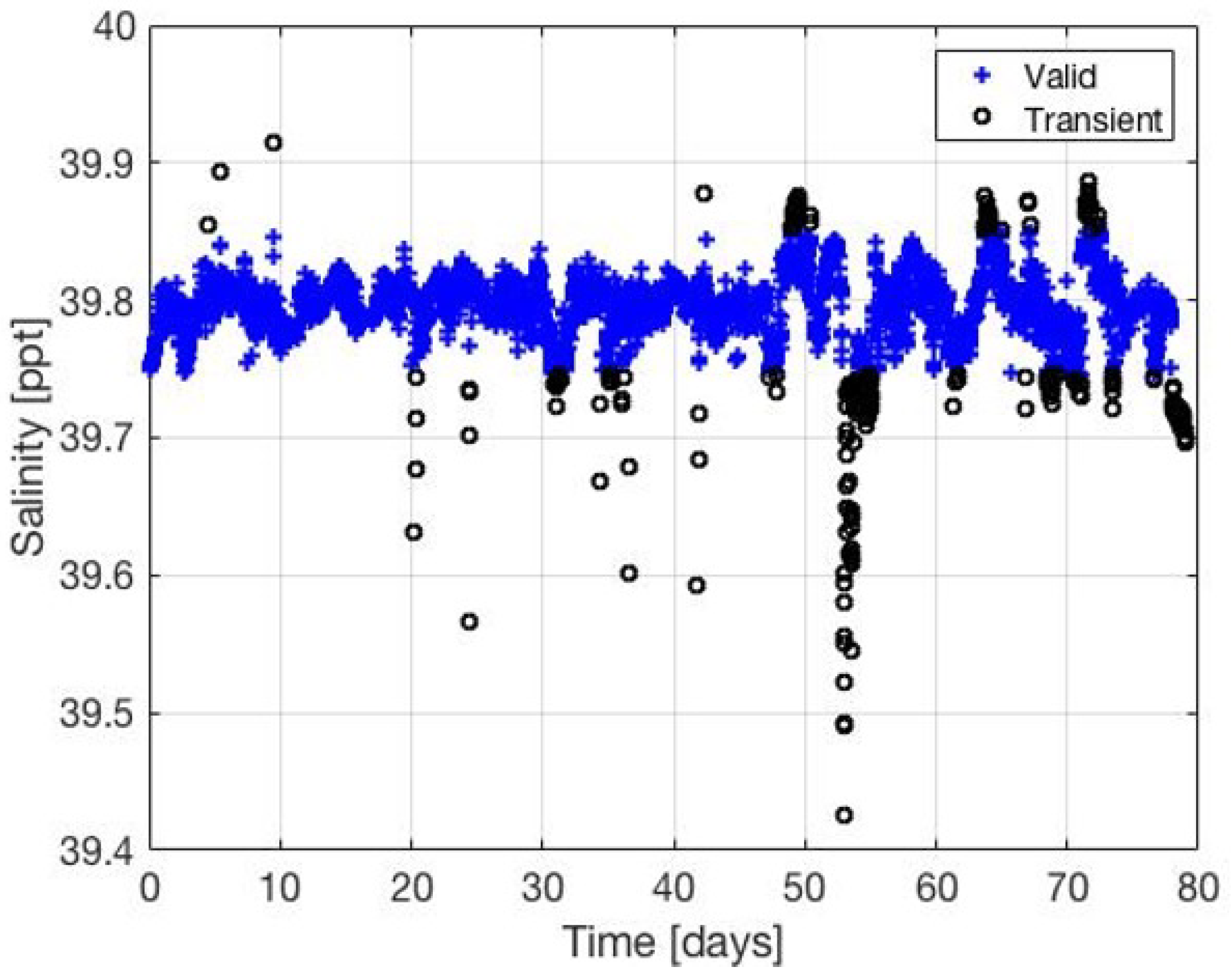
We determine a group of datasets to be related to the examined one if from (4) is below a threshold . To accommodate the above Type I and Type II of similarities, the above process is repeated for the raw data and for the wavelet transformed version of it. An example for the classification into ‘valid’ and ‘anomaly’ of a salinity dataset using predictions from the water temperature dataset over a period of 80 days is shown in Figure 4. We observe that anomalies are detected well by comparison between the predicted (valid) samples and the full original dataset.
3.2. Online: Identifying Faulty Data Samples
3.2.1. Anomaly Detection
As the focus of this work is on QA verification, we avoid suggesting a new technique for anomaly detection. Instead, as benchmarks, we follow the procedure in [7] for the definition of a Spike Test and Gradient Test as two different methods for identifying anomalies. A spike is a rapid and temporary change in value whose probability of occurrence is low. In the frequency domain, a spike will appear as a short wideband signal of high or low intensity. In turn, a gradient change is a difference in the value of the tangent vector that reflects a change in the directional sample-wise derivative of the dataset. Formally, for a set of data samples and a tested value , the spike test aims to identify a sample that stands out from its local environment and is defined by
The gradient test identifies outliers and is set by
To detect an anomaly, both the above tests were compared to dataset-specific detection thresholds.
3.2.2. Detection Verification
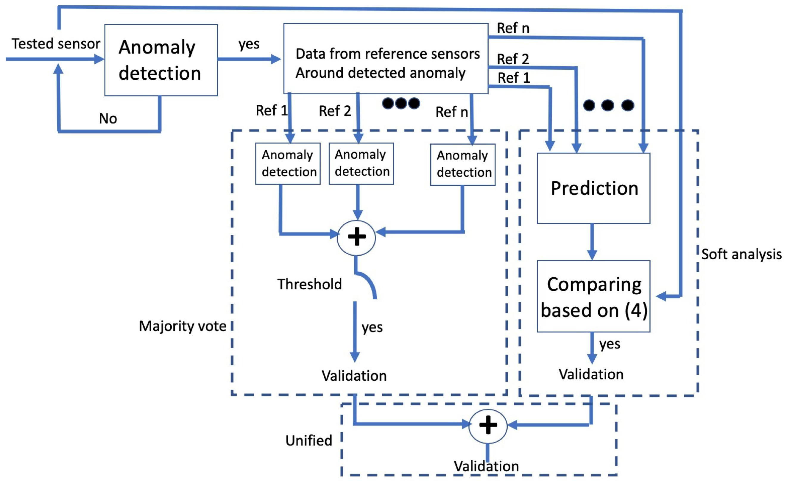
Once an anomaly is detected within the examined dataset, verification is performed. Verification is based on the comparison between the examined dataset and its related datasets within the time frame where the anomaly was detected. We consider two approaches: (1) majority vote, and (2) soft analysis. A unified combination of these two is also possible.
Referring to the illustration in Figure 5, in majority vote each data sample in a related dataset is tested separately for the presence of a corresponding anomaly. Define as the time at which an anomaly was found in the examined dataset, and let be a corresponding time window around . An anomaly is verified only if an anomaly is also detected within by more than r related datasets. The value for can be widened to consider delays between the effect of physical phenomena as it gets reflected in different datasets, or narrowed to avoid misalignment between datasets. In our analysis below, we set to be 30 min, which allows a window of 3 samples on average, and, for three related datasets, we consider .
The hard decision approach of the majority vote holds the advantage of eliminating the flagging of valid transients as false, but cannot manage the case of hardware malfunction of sensors where data is false at all datasets. Further, because each dataset is analyzed separately, this approach does not utilize the relationship between all the related datasets. For these cases we offer a soft analysis approach, where data samples from all related datasets are combined. A matrix of data samples from all related datasets within serves as an input to an SVR whose output is a prediction of the examined dataset at , i.e., the anomaly. This is the same SVR as trained during the offline step to identify the related datasets. The anomaly identified from the examined data sample is then considered valid if the prediction is successful, i.e., in (4) exceeds threshold . Since a faulty data sample is not expected to allow accurate prediction, the soft analysis approach can discover batches of samples where all sensors produced faulty data.
4. Results
In this section, we explore the results of our cross-sensor QA scheme for the surface water temperature dataset measured at the THEMO observatory. As a baseline to evaluate our results, we have used an expert to hand-label the examined dataset. Out of 5520 observed samples taken over a period of 7 months, the labeling identified 328 anomalies.
As benchmarks, we compared the performance of our cross-sensor approach with the spike and gradient anomaly detectors offered in [7] and described in (5) and (6), respectively. As spikes are easily observed in the time domain, for the spike test we use raw measurements. Contrarily, since gradients are harder to observe, for the gradient test we use the wavelet transform that highlights high-frequency components. Performance are explored for the majority vote and the soft analysis approaches. For the former, the same spike or gradient test used for the benchmark is passed over the found related datasets using the same detection threshold.
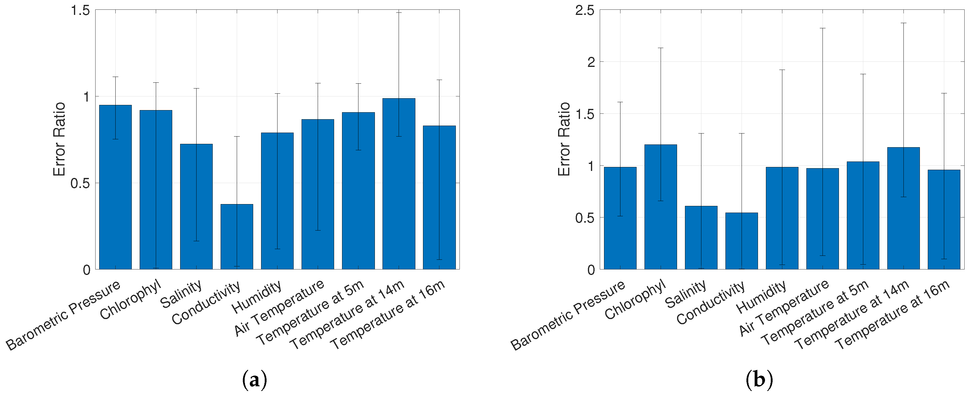
To identify the list of related datasets, we examined the nine datasets in Table 1, namely, salinity, chlorophyll, conductivity, barometric pressure, humidity, air temperature and water temprature at three different depths (see also Figure 2). Results in Figure 6a,b shows the ratio between the prediction error obtained when using all nine possible related datasets and the error obtained when removing one dataset. The rational behind this exploration is to quantify the contribution of a single dataset for the overall prediction task. Formally, for an examined data sample x and its predictions, and , where is the entire set of considered related datasets and is the entire set without the j-th dataset, respectively, we measure
It is expected that the prediction error obtained when using a single dataset would be higher than when using the entire dataset.
The results shown in Figure 6a,b identify the salinity, conductivity, and humidity datasets as the related datasets when raw data is considered, and the salinity and conductivity datasets as the related datasets when the wavelet transform of the datasets are analyzed. We note that using the above group of related sensors, , the absolute prediction error during testing, , is 0.08 C. Considering that the examined temperature dataset lies between 19 and 30.6 C, with a standard deviation of 3.9 C, we argue that this is a sufficiently accurate prediction. This strengthens our claim for the diversity gain obtained when utilizing cross-sensor information. In the below, we use only these identified datasets as the related set.
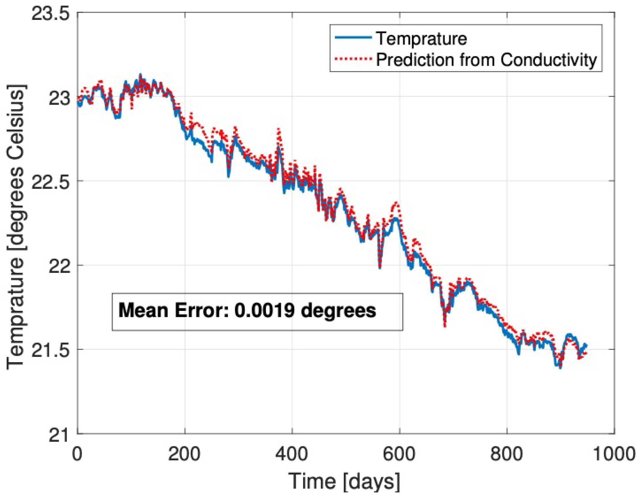
An example of the prediction obtained by SVR of the surface temperature dataset from the conductivity dataset is shown in Figure 7. Both datasets were recorded by the THEMO observatory over a period of 900 days. The prediction closely resembles the decreasing trend in time for the examined dataset, and it is shorter (tens of days) term transient variability. To quantify this, the surface temperature data samples and their prediction can be fitted, respectively, with the following linear trends
with close R-squared values of 0.972 and 0.97, respectively, a cross-correlation of 0.9983, and a p-value of 0 for testing the hypothesis of no correlation between the two datasets. The obtained mean error of the prediction, defined by the Euclidean distance
between the examined data sample, x, and its prediction, , has a value of 0.0019 C, which is extremely small with respect to the apparent transient variability of the examined dataset. Some prominent transients in the original water temperature dataset are also observed in the predicted dataset, for example, on day 380 and around day 600. In contrast to standard methods, the cross-sensor criteria show that these are valid data samples. Consequentially, our approach avoids classifying these samples as anomalies.
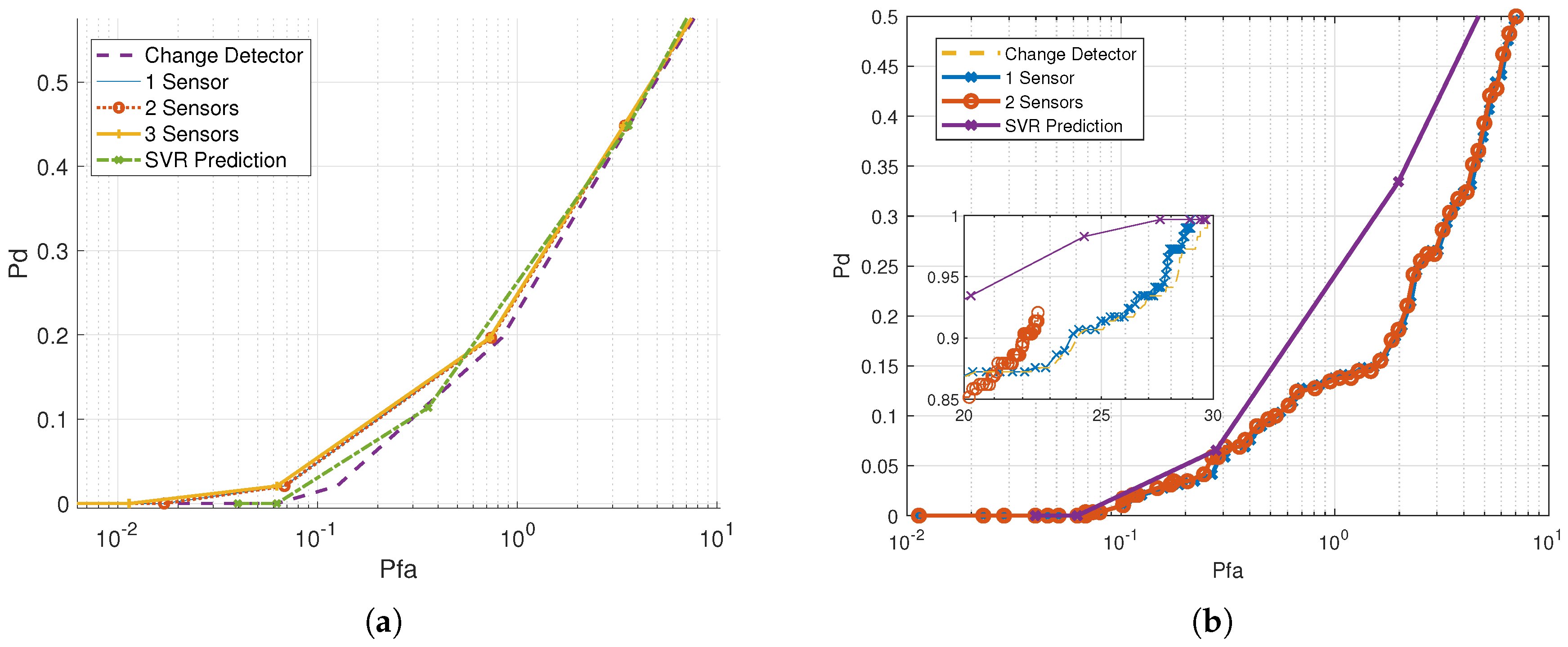
Results in terms of the receiving operating characteristics (ROC) with respect to the expert labeling are shown in Figure 8a,b for the gradient and spike tests, respectively. The former is computed for the raw data and the latter for the wavelet transform of the data. Pairs of false alarm vs. correct detection rate are obtained by changing the detection threshold. False alarm values are calculated as the count of samples falsely determined to be erroneous, and results are normalized by the number of data samples examined per day. Detection probability is counted as the percentage of correctly identified anomalies out of all expert tagged valid anomalies. We show results for the majority vote (marked by x-Sensor, with reflecting the number of related datasets required for the majority decision) and for the soft analysis (marked by SVR-Prediction). These are compared with the per-sensor anomaly detection (marked by Change-Detector that serves as a benchmark.
As expected, adding verification to the anomaly detection benchmark reduces the false alarm rate at the cost of a decrease in the detection rate. However, examining the trade-off between the two metrics (considered better the more ‘left’ the curve in the ROC is), we note that, compared to the per-sensor anomaly detection, improved performance are obtained for our cross-sensor validation approach. For example, in the gradient test on the raw dataset (Figure 8a) and for a detection rate of 0.2, the false alarm rate reduces from 0.83 per day for the per-sensor QA to 0.72 for the majority vote (three sensors) and to 0.65 for the soft analysis SVR prediction. Similarly, for the spike test on the wavelet transform of the dataset (Figure 8a) and for a detection rate of 0.2, the false alarm rate reduces from 2.15 per day for the per-sensor QA to 2.09 for the majority vote (2 sensors) and to 0.743 for the SVR prediction. Comparing the two QA verification approaches, we conclude that the soft analysis using the SVR prediction achieves better results than the majority vote. This is mostly because the SVR is able to fuse datasets rather than comparing hard decisions by the majority vote, and thus obtains higher diversity gain. This gain is shown to be more significant in the case of the spike test over the wavelet transform. This is because the SVR classifier is able to capture better differences in datasets that are highlighted by the wavelet transform.
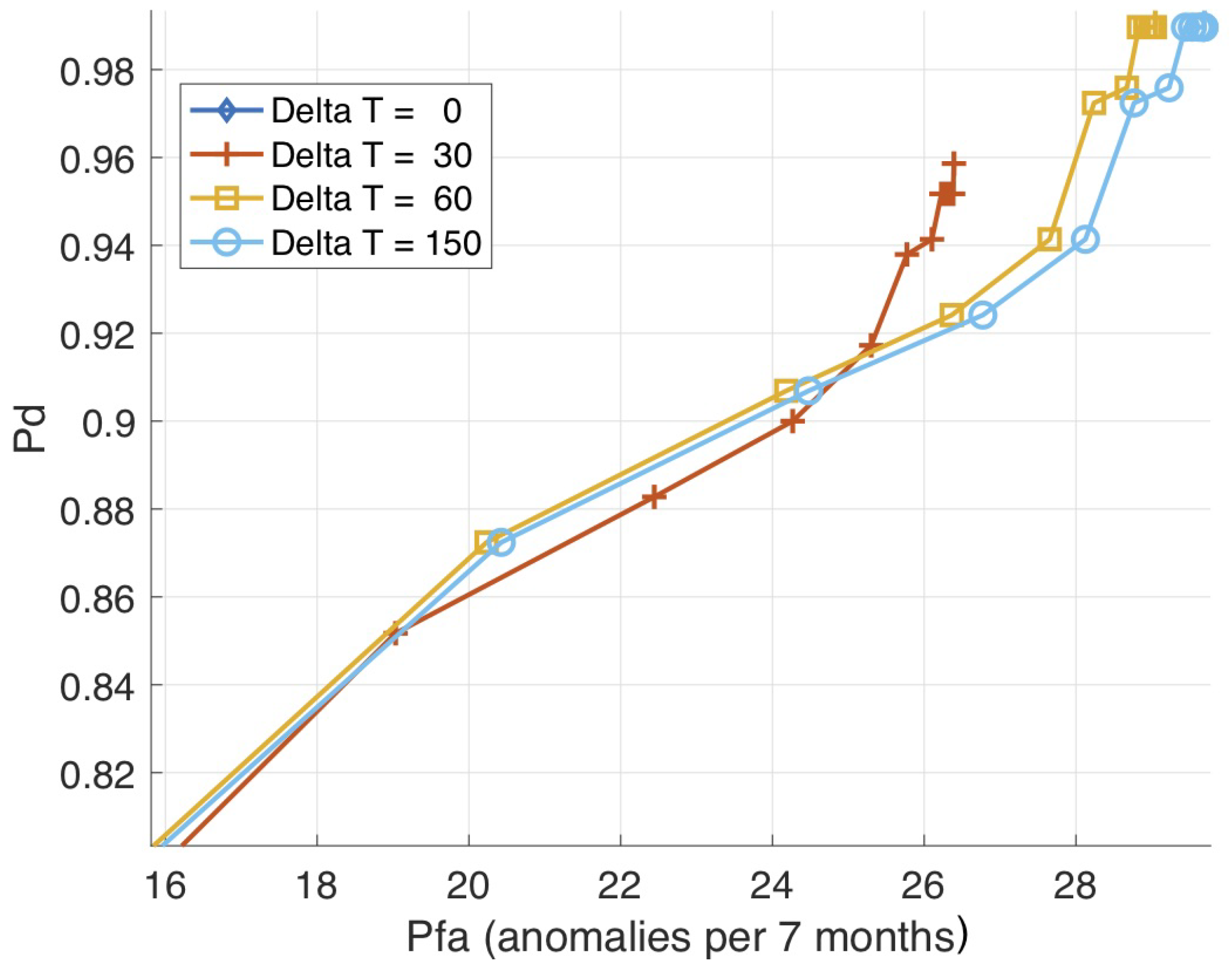
Finally, in Figure 9 we explore the influence on performance of the time-frame parameter, . For different values of , we show the ROC results of the majority vote approach using the spike test (6) as a benchmark. The results show that the choice of min yields the best performance. However, the difference in performance for other choices of are negligible, which suggests that, within reasonable values, our approach is robust with respect to the choice of the parameter.
5. Discussion
Our method for QA validation is designed to decrease the false identification rate, , of anomalies in the examined dataset at a small cost of a decrease in the correct identification rate, . Compared with the two benchmark schemes from [7], the results show that our approach yields a favorable trade-off for the and objectives, such that, for a given , less false identifications of anomalies are made. As we demonstrated for the surface water temperature dataset collected by THEMO, such false identifications of anomalies are common, yielding the discrimination of important samples that are sometimes key for understanding temporal phenomena. Our approach, thus, not only approves more data samples for analysis, but more importantly, avoids neglecting valid anomalies that may correspond to short-term physical phenomena that are of high importance.
Our solution is general in principle and can be applied for any marine observatory or station including multiple sensors of various kinds. However, it has some limitations. First, the sensors must be at an approximate location and sample the same water body; second, data samples must be obtained simultaneously at roughly the same time instance; third, the datasets should be a time-series so to allow the identification of anomalies. Finally, the geographical area explored must be stable enough such that different physical phenomena could be related.
Our results showed that validation by SVR prediction offers better performance than the majority vote. This result was explained by the capability of the SVR to capture non-linear relations between different datasets. We, therefore, expect that results would improve the more related the datasets are. Thus, one way to enhance performance is to train the SVR separately per-season. Since oceanographic datasets tend to considerably change between seasons, a per-season analysis has the potential to better capture the relationships between the explored datasets. Furthermore, a unified validation that combines decisions made by the majority vote and by the soft analysis may produce better results. Since in this work we focus on introducing the concept of cross-sensor validation, we leave this investigation for future work.
6. Conclusions
In this paper, we explored the use of multiple sensors for the task of validating quality assurance (QA) decisions for datasets from a marine observatory. Different than the existing methods that perform QA for each dataset separately, we utilize the likely relationships among different datasets probing the same water body as a form of spatial diversity. For each examined dataset, our approach identifies a group of datasets whose data samples can be used for the prediction of the examined dataset. We use this group of related datasets to validate each anomaly identified in the examined dataset. We offer two approaches: a majority vote in which an anomaly detection is determined valid only if anomalies are not found in the related datasets, and a soft decision approach using SVR prediction where an anomaly is approved if it cannot be predicted from the corresponding list of related datasets. Results from our marine observatory, THEMO, comparing our cross-sensor approach to two per-sensor anomaly detectors demonstrate a favorable trade-off for decreasing the false alarm rate at the cost of a slight increase in the detection rate.
Author Contributions
Conceptualization, R.D.; methodology, R.D. and I.S.; software, I.S.; validation, R.D., B.M.F. and Y.M.; formal analysis, R.D. and N.A.C.; investigation, Y.M. and N.A.C.; resources, R.D., Y.M. and N.A.C.; data curation, I.S.; writing—original draft preparation, R.D.; writing—review and editing, Y.M., B.M.F. and N.A.C.; visualization, R.D. and I.S.; supervision, R.D. and N.A.C.; project administration, R.D. and N.A.C.; funding acquisition, R.D., Y.M. and N.A.C. All authors have read and agreed to the published version of the manuscript.
Funding
This research was funded by the Israel and Portugal Ministries of Science grants number 3-16525 and PT-IL/0002/2019.
Conflicts of Interest
The authors declare no conflict of interest.
Appendix A. Guidelines for Anticipating Related Datasets
Relationships among the different oceanographic measurables are diverse. For example, rain should be associated with a decrease in conductivity that is measured close to the surface. A more complex relationship exists in the case of upwelling, where a consistent along-coast wind eventually causes surface water to be displaced off-shore, bringing colder, high nutrient water upwards. Alternatively, there are other cases where the mechanisms are complex. For example, there are many factors affecting the dynamics of algae blooms with variable levels of influence. However, the general consensus is that algae blooms are usually the combined result of high nutrient availability with optimal temperature and light conditions. In this case, a turbidity sensor, for example, may play a dual role before and after the event. In calm waters and low turbidity, the light would penetrate deeper and foster the rapid multiplication of algae, and in turn resulting in an increase in turbidity and, eventually, oxygen depletion.
The identification of related datasets can be done in two basic alternative approaches. The first is to exploit the physical, chemical and/or biological relationships between the different environmental measurables, as modeled through a range of methodologies. At one end of this range are pre-known relations that can be explicitly computed directly from the different measured values. The primary example is the equation of state, relating the potential temperature, salinity and density within a specific water mass away from its boundaries. Within the range of methodologies is the use of a-priory models to resolve the variability of the relations. An example is the use of typical seasonal vertical profiles of oceanic measurables to define the boundaries of water masses and help asses measurements taken near and across boundaries. At the end of this spectrum of methodologies is the utilization of dynamic synoptic models to relate the measurables expected. An example is the relationship between temperature measurements and current measurements, related through water turbulence in response to the temperature field. The second, alternative, basic approach is to derive empiric relationships among different measured datasets by analyzing data accumulated in these datasets at the measurement site or region. Such analysis can have manual components or be entirely automatic, and normally would evaluate the dependence on additional basic parameters, such as the hour, season and depth. These empirical relations can be improved as data accumulates.
References
- Walpert, J.; Guinasso, N.; Lee, W.; Liu, D.; Buschang, S. TABS responder—A quick response buoy to supplement the TABS network. In Proceedings of the 2014 Oceans-St. John’s, St. John’s, NL, Canada, 14–19 September 2014; pp. 1–6. [Google Scholar]
- Cooke, S.; Iverson, S.; Stokesbury, M.; Hinch, S.; Fisk, A.; VanderZwaag, D.; Apostle, R.; Whoriskey, F. Ocean Tracking Network Canada: A network approach to addressing critical issues in fisheries and resource management with implications for ocean governance. Fisheries 2011, 36, 583–592. [Google Scholar] [CrossRef]
- Diamant, R.; Knapr, A.; Dahan, S.; Mardix, I.; Walpert, J.; DiMarco, S. THEMO: The Texas A&M-University of Haifa-Eastern Mediterranean Observatory. In Proceedings of the 2018 OCEANS-MTS/IEEE Kobe Techno-Oceans (OTO), Kobe, Japan, 28–31 May 2018; pp. 1–5. [Google Scholar]
- Koziana, J.; Olson, J.; Anselmo, T.; Lu, W. Automated data quality assurance for marine observations. In Proceedings of the OCEANS 2008, Quebec City, QC, Canada, 15–18 September 2008; pp. 1–6. [Google Scholar]
- Biffard, B.; Morley, M.; Hoeberechts, M.; Rempel, A.; Dakin, T.; Dewey, R.; Jenkyns, R. Adding value to big acoustic data from ocean observatories: Metadata, online processing, and a computing sandbox. J. Acoust. Soc. Am. 2018, 144, 1956. [Google Scholar] [CrossRef]
- Quality Control of Ocean Observatory Initiative. 2018. Available online: https://oceanobservatories.org/quality-contro (accessed on 1 June 2020).
- Abeysirigunawardena, D.; Jeffries, M.; Morley, M.; Bui, A.; Hoeberechts, M. Data quality control and quality assurance practices for Ocean Networks Canada observatories. In Proceedings of the OCEANS 2015-MTS/IEEE Washington, Washington, DC, USA, 19–22 October 2015; pp. 1–8. [Google Scholar]
- Wong, A.; Keeley, R.; Carval, T. Argo Quality Control Manual for CTD and Trajectory Data, Version 3.1; Technical report; IFREMER: Brest, France, 16 January 2018. [Google Scholar] [CrossRef]
- Batsi, E.; Tsang-Hin-Sun, E.; Klingelhoefer, F.; Bayrakci, G.; Chang, E.T.; Lin, J.Y.; Dellong, D.; Monteil, C.; Géli, L. Nonseismic Signals in the Ocean: Indicators of Deep Sea and Seafloor Processes on Ocean-Bottom Seismometer Data. Geochem. Geophys. Geosyst. 2019, 20, 3882–3900. [Google Scholar] [CrossRef]
- Diamant, R.; Dahan, S.; Mardix, I. Communication Operations at THEMO: The Texas A&M - University of Haifa - Eastern Mediterranean Observatory. In Proceedings of the 2018 Fourth Underwater Communications and Networking Conference (UComms), Lerici, Italy, 28–30 August 2018; pp. 1–5. [Google Scholar]
- Howe, B.; Chan, T.; El-Sharkawi, M.; Kenney, M.; Kolve, S.; Liu, C.; Lu, S.; McGinnis, T.; Schneider, K.; Siani, C.; et al. Power System for the MARS Ocean Cabled Observatory. In Proceedings of the Scientific Submarine Cable 2006 Conference, 2006; pp. 7–10. Available online: http://neptunepower.apl.washington.edu/publications/documents/psftmoco.pdf (accessed on 19 October 2020).
- Bushnell, M.; Kinkade, C.; Worthington, H. Manual for Real-Time Quality Control of Ocean Optics Data: A Guide to Quality Control and Quality Assurance of Coastal and Oceanic Optics Observations. 2017. Available online: file:///Users/Downloads/noaa_20938_DS1.pdf (accessed on 1 June 2020).
- Bushnell, M.; Worthington, H. Manual for Real-Time Quality Control of Wind Data: A Guide to Quality Control and Quality Assurance for Coastal and Oceanic Wind Observations. 2017. Available online: https://repository.library.noaa.gov/view/noaa/15487 (accessed on 1 June 2020).
- Timms, G.; Souza, P.D.; Reznik, L.; Smith, D. Automated data quality assessment of marine sensors. Sensors 2011, 11, 9589–9602. [Google Scholar] [CrossRef] [PubMed] [Green Version]
- Lévy, M.; Ferrari, R.; Franks, P.; Martin, A.; Rivière, P. Bringing physics to life at the submesoscale. Geophys. Res. Lett. 2012, 39, 1–13. [Google Scholar] [CrossRef] [Green Version]
- McWilliams, J. Submesoscale currents in the ocean. Proc. R. Soc. A Math. Phys. Eng. Sci. 2016, 472, 20160117. [Google Scholar] [CrossRef] [PubMed]
- Talley, L. Descriptive Physical Oceanography: An Introduction; Academic Press: Cambridge, MA, USA, 2011. [Google Scholar]
- Datasets Used for Analysis and Their Tagging. 2020. Available online: https://drive.google.com/drive/folders/1SDoV8wejlpYtn3hBrYlw0uej5vmMHJqC?usp=sharing (accessed on 1 October 2020).
- Mamayev, O. Temperature-Salinity Analysis of World Ocean Waters; Elsevier: Amsterdam, The Netherlands, 2010. [Google Scholar]
- Emery, W.; Meincke, J. Global water masses-summary and review. Oceanol. Acta 1986, 9, 383–391. [Google Scholar]
- Rudnick, D.; Ferrari, R. Compensation of horizontal temperature and salinity gradients in the ocean mixed layer. Science 1999, 283, 526–529. [Google Scholar] [CrossRef] [PubMed] [Green Version]
- Rudnick, D.; Martin, J. On the horizontal density ratio in the upper ocean. Dyn. Atmos. Ocean. 2002, 36, 3–21. [Google Scholar] [CrossRef]
- Abraham, E. The generation of plankton patchiness by turbulent stirring. Nature 1998, 391, 577–580. [Google Scholar] [CrossRef]
- Bouman, H.; Platt, T.; Sathyendranath, S.; Li, W.; Stuart, V.; Fuentes-Yaco, C.; Maass, H.; Horne, E.; Ulloa, O.; Lutz, V.; et al. Temperature as indicator of optical properties and community structure of marine phytoplankton: Implications for remote sensing. Mar. Ecol. Prog. Ser. 2003, 258, 19–30. [Google Scholar] [CrossRef]
- Eckart, C. Properties of water, Part II: The equation of state of water and sea water at low temperatures and pressure. Am. J. Sci. 1958, 256, 225–240. [Google Scholar] [CrossRef]
- Bryan, K.; Cox, M. An approximate equation of state for numerical models of ocean circulation. J. Phys. Oceanogr. 1972, 2, 510–514. [Google Scholar] [CrossRef]
- Riera-Guasp, M.; Antonino-Daviu, J.; Pineda-Sanchez, M.; Puche-Panadero, R.; Pérez-Cruz, J. A general approach for the transient detection of slip-dependent fault components based on the discrete wavelet transform. IEEE Trans. Ind. Electron. 2008, 55, 4167–4180. [Google Scholar] [CrossRef]
- Abu, A.; Diamant, R. A Statistically-Based Method for the Detection of Underwater Objects in Sonar Imagery. IEEE Sens. J. 2019, 19, 6858–6871. [Google Scholar] [CrossRef]
- Diamant, R.; Campagnaro, F.; de Filippo de Grazia, M.; Casari, P.; Testolin, A.; Sanjuan Calzado, V.; Zorzi, M. On the Relationship Between the Underwater Acoustic and Optical Channels. IEEE Trans. Wirel. Commun. 2017, 16, 8037–8051. [Google Scholar] [CrossRef]
- Cortes, C.; Vapnik, V. Support-vector networks. Mach. Learn. 1995, 20, 273–297. [Google Scholar] [CrossRef]
- Smola, A.; Schölkopf, B. A tutorial on support vector regression. Stat. Comput. 2004, 14, 199–222. [Google Scholar] [CrossRef] [Green Version]
- Kokare, M.; Chatterji, B.; Biswas, P. Comparison of similarity metrics for texture image retrieval. In Proceedings of the Conference on Convergent Technologies for Asia-Pacific Region (TENCON), Bangalore, India, 15–17 October 2003; Volume 2, pp. 571–575. [Google Scholar]
Figure 1.
Temperature data at three water depth measured in THEMO. Some anomalies in temperature are shown to correlate at different depths (example marked by the purple-dashed arrow), while others exist only at a single depth (example marked by the green-solid arrow).
Figure 1.
Temperature data at three water depth measured in THEMO. Some anomalies in temperature are shown to correlate at different depths (example marked by the purple-dashed arrow), while others exist only at a single depth (example marked by the green-solid arrow).

Figure 2.
Dependencies between datasets measured in THEMO.

Figure 3.
A time-series (blue) of the surface water temperature recorded by THEMO over the selected time frame (the examined dataset), with the anomalies tagged by an expert marked (red).
Figure 3.
A time-series (blue) of the surface water temperature recorded by THEMO over the selected time frame (the examined dataset), with the anomalies tagged by an expert marked (red).

Figure 4.
Classification of a THEMO salinity dataset into valid (blue plus marks) and transient (black circles) data using predictions from a water temperature dataset.
Figure 4.
Classification of a THEMO salinity dataset into valid (blue plus marks) and transient (black circles) data using predictions from a water temperature dataset.

Figure 5.
Illustration of the detection verification approaches.

Figure 6.
The ratios between the prediction errors (7) when using all N possible related datasets vs. when using a subset of datasets. The bar labels (bottom) indicate the removed dataset in each of the cases, bar level indicates the mean value while error bars represent the 95% confidence interval. (a) Raw dataset. (b) After wavelet transform.

Figure 7.
THEMO water temperature data (blue) and its prediction from conductivity data (red), as obtained by the support vector regression (Radial Basis Function (RBF) kernel) method.
Figure 7.
THEMO water temperature data (blue) and its prediction from conductivity data (red), as obtained by the support vector regression (Radial Basis Function (RBF) kernel) method.

Figure 8.
Receiver operating characteristics (ROC) results shown for standard anomaly detection (change detector) and for cross-sensor validation—majority vote for anomaly agreement by 1, 2 and 3 datasets, and soft-analysis by support virtual regression (SVR). (a) A gradient test for raw data. (b) Spike test for wavelet transform over the data.

Figure 9.
ROC results of majority vote using the spike test as a function of .


Table 1.
Spesification of sensors used for data analysis.
| Description | Sensor Model |
|---|---|
| Barometric pressure [mbars] (3 m above sea surface) | Vaisala (PTB210) |
| Chlorophyll [µg/L] (depth 1 m) | Wet Labs (ECOFLNTUS) |
| Salinity [PSU] (depth 1 m) | CTD microcat (SBE37-SI) |
| Conductivity [S/m] (depth 1 m) | CTD microcat (SBE37-SI) |
| Temperature [C] (depth 1 m) | CTD microcat (SBE37-SI) |
| Air humidity [RH%] (3 m above sea surface) | Rotronics (mp101a) |
| Air temperature [C] (3 m above sea surface) | Rotronics (mp101a) |
| Temperature [C] (depths 5 m, 14 m, 16 m) | Sound-nine (Ulti-Modem) |
Publisher’s Note: MDPI stays neutral with regard to jurisdictional claims in published maps and institutional affiliations. |
© 2020 by the authors. Licensee MDPI, Basel, Switzerland. This article is an open access article distributed under the terms and conditions of the Creative Commons Attribution (CC BY) license (http://creativecommons.org/licenses/by/4.0/).
Share and Cite
MDPI and ACS Style
Diamant, R.; Shachar, I.; Makovsky, Y.; Ferreira, B.M.; Cruz, N.A. Cross-Sensor Quality Assurance for Marine Observatories. Remote Sens. 2020, 12, 3470. https://0-doi-org.brum.beds.ac.uk/10.3390/rs12213470
AMA Style
Diamant R, Shachar I, Makovsky Y, Ferreira BM, Cruz NA. Cross-Sensor Quality Assurance for Marine Observatories. Remote Sensing. 2020; 12(21):3470. https://0-doi-org.brum.beds.ac.uk/10.3390/rs12213470
Chicago/Turabian StyleDiamant, Roee, Ilan Shachar, Yizhaq Makovsky, Bruno Miguel Ferreira, and Nuno Alexandre Cruz. 2020. "Cross-Sensor Quality Assurance for Marine Observatories" Remote Sensing 12, no. 21: 3470. https://0-doi-org.brum.beds.ac.uk/10.3390/rs12213470
Note that from the first issue of 2016, this journal uses article numbers instead of page numbers. See further details here.